ISSN 1751-8644 Discrete-time non-linear state observer

1

6

11

16

21

26

31

36

41

46

51

56

61

66

71

76

81

86

91

96

101

106

111

116

121

126

131

136

www.ietdl.org

Published in IET Control Theory and ApplicationsReceived on 7th September 2012Revised on 1st October 2013Accepted on 1st December 2013doi: 10.1049/iet-cta.2013.0568

ISSN 1751-8644

Techset Composition Ltd, Salisbury Doc: {IEE} CTA20130568.tex

Discrete-time non-linear state observer based on asuper twisting-like algorithmIván Salgado1, I. Chairez2, Bijnan Bandyopadhyay3, Leonid Fridman4 and Oscar Camacho1

1CIC, Instituto Politecnico Nacional, Mexico City, Mexico2Department of Bioprocesses, UPIBI, Instituto Politecnico Nacional, Mexico City, Mexico3 SYSCON, Indian Institute ofTechnology, Bombay, Mumbai, India4Engineering Universidad Nacional Autonoma de Mexic, Mexico City, MexicoE-mail: [email protected]

Abstract: The properties of robustness and finite-time convergence provided by sliding mode (SM) theory have motivatedseveral researches to deal with the problems of control and state estimation. In the SM theory, the super-twisting algorithm(STA), a second-order SM scheme, has demonstrated remarkable characteristics when it is implemented as a controller,observer or robust signal differentiator although the presence of noise and parametric uncertainties. However, the design ofthis algorithm was originally developed for continuous-time systems. The growth of microcomputers technology has attractedthe attention of researchers inside the SM discrete-time domain. Recently, discretisations schemes for the STA were studiedusing majorant curves. In this study, the stability analysis in terms of Lyapunov theory is proposed to study a discrete-timesuper twisting-like algorithm (DSTA) for non-linear discrete-time systems. The objective is to preserve the STA characteristicsof robustness in a quasi-sliding mode regime that was proved in terms of practical Lyapunov stability. An adequate combinationof gains obtained by the same Lyapunov analysis forces the convergence for the DSTA. The problem of state estimationis also analysed for second-order mechanical systems of n degrees of freedom. Simulation results regarding the design of asecond-order observer using the DSTA for a simple pendulum and a biped model of seven degrees of freedom are presented.

1 Introduction

Nowadays, the advance in the development of microcon-

Q1

trollers with capabilities to solve advanced mathematicalalgorithms has allowed the implementation of complex con-trol schemes without the use of personal computers. In thisway, the requirement of control and state estimation strate-gies downloadable in these microcontrollers has oriented theresearch of control strategies in two principal frameworks.The first one analyses the discretisation problem of sev-eral control techniques and its sampled time dependencesin the discrete-time domain. On the other hand, as the sec-ond framework, new control strategies have been presentedto study the case of pure discrete-time systems. These tech-niques include the well-known sliding mode (SM) theory[1]. In addition, the implementation of integration schemescould be an option to keep working with continuous strate-gies. However, the computational requirements are increasedwhen this option is implemented.

The SM theory has been widely applied to solve thestate estimation problem. The main features obtained by SMare robustness against parametric uncertainties and finite-time convergence. These advantages are evident in contrastwith the conditions required for non-linear systems whena classical structure for observation is used, like a Luen-berger one. Indeed, the necessity of the exact mathematical

description constitutes a drawback in this kind of algo-rithms. Following the idea of Luenberger structures, theso-called high-gain observers have been developed to dealwith complex non-linear systems [2].

Sliding motion is obtained by including a discontinuityterm in the algorithm structure. The discontinuous injectionmust be designed such that the trajectories of the system areforced to remain on a prescribed submanifold (sliding sur-face) on the state space. The resulting motion in the surfaceis named as a sliding motion [3, 4]. If the system has relativedegree greater than one with respect to the sliding surface,high-order sliding modes (HOSM) such as the second-ordersliding modes (SOSM) could be implemented preserving themain characteristics of classical SM [5, 6]. Moreover, SOSMreduce the undesired chattering effect. In continuous-time,the super-twisting algorithm (STA) has been successfullyanalysed and applied like a robust exact differentiator [7],state estimator [8] or controller [9]. Although, there existseveral researches in the continuous domain, the conceptof high-order discrete-time sliding modes (DSM) has notdeeply studied.

DSM have not received much attention as the continu-ous counterpart. The first ideas of DSM were introducedin [10, 11], where a quasi-sliding mode (QSM) is estab-lished for systems with relative degree one. In [12], the studyof discrete-time single-input single-output (SISO) non-linear

IET Control Theory Appl., pp. 1–10 1doi: 10.1049/iet-cta.2013.0568 © The Institution of Engineering and Technology 2014

141

146

151

156

161

166

171

176

181

186

191

196

201

206

211

216

221

226

231

236

241

246

251

256

261

266

271

276

www.ietdl.org

systems with relative degree bigger than one was consid-ered. A new definition of the QSM regime was addressed in[13]. In this paper, the motion of the system was restrictedin a certain band around the sliding surface. In [14, 15]some researches have been reported for several classes ofdiscrete-time linear systems. The idea of SOSM control indiscrete-time systems was introduced in terms of a certainclasses of discretisation-like Euler discretisation or finite dif-ferences [8, 16, 17]. However, a complete stability study hasnot been deeply analysed in terms of Lyapunov stability.

There are several generic methods for designing slid-ing mode observers (SMO). For continuous-time linear andnon-linear systems, most of these observers are based onthe equivalent control concept for handling disturbancesand modelling uncertainties. In the same context, discrete-time sliding mode control (DSMC) methods have alsobeen developed for linear and non-linear systems [12, 18,19]. However, discrete-time sliding mode-based observer(DSMO) design has not received much attention, especiallyfor non-linear systems. DSMO design for linear systemswas given in [18]. In [20], the concept of sliding latticefor discrete-time systems was introduced and DSMO wasdesigned for SISO linear systems using the Lyapunov min–max method. Besides, in several works the accuracy ofthe discretisation in SOSM controllers depending on thesampling period has been analysed [21, 22].

In this paper, a discrete-time SOSM algorithm is proposedbased on the well known STA. Stability of discrete-timesuper twisting-like algorithm (DSTA) is analysed with aquadratic Lyapunov function. Stability conditions for theDSTA were obtained with the solution of a linear matrixinequality (LMI) and the trajectories were confined into aboundary layer in the vicinity of the sliding surface and staysinside it forever obeying a QSM behaviour. The boundarylayer magnitude is proportional to the square of the sampledperiod. A natural application for the DSTA as a second orderdiscrete-time observer is analysed under the same strategy.This analysis was done using quadratic Lyapunov functionsan LMI techniques.

In the following section, the structure of the DSTA isgiven. The result regarding the convergence of the pro-posed algorithm is established in terms of a simple quadraticLyapunov function in Section III. In Section IV, numericalexamples are presented. The first example is based on thestate estimation problem of a Furuta pendulum and a sec-ond one to estimate the states of a biped model with sevendegrees of freedom. Finally, in Section V, some conclusionsare established.

2 Discrete-time super-twisting-likealgorithm

The DSTA is composed by the following two equations indifferences

x1(k + 1) = ρ1x1(k) + τx2(k)−τk1|x1(k)|1/2sign(x1(k))

x2(k + 1) = ρ2x2(k) − τk2sign(x1(k))(1)

where xi(k) ∈ � are the states, ρi ∈ �+, |ρi| < 1, ki ∈ � fori = 1, 2, are the gains to be designed for ensuring the conver-gence of (1) to the origin and τ > 0 is the sampling period.

The sign(κ) function is defined as

sign(κ) :=⎧⎨⎩

−1 if κ < 00 if κ = 01 if κ > 0

(2)

where κ ∈ �.Equation in (1) is designed as a slightly modification of an

Euler discretisation from the continuous SOSM. The system(1) can be represented as

x(k + 1) = Ax(k) + B(k)sign(x1(k)) (3)

where A ∈ �2×2 and B(k) ∈ �2 are

A :=[ρ1 τ0 ρ2

]B(k) :=

[−τk1 |x1(k)|1/2

−τk2

](4)

2.1 Main result

The result obtained in this paper is stated in the followingtheorem.

Theorem 1: Consider the non-linear system given in (1),with gains selected as k1> 0 and k2 > 0 and if the followingLMI

A�(P + P�P)A−(1 − �)P + Q≤ 0 (5)

has a positive-definite solution P = P� > 0 for a givenQ = Q� > 0 and � = �� > 0, then, the trajectories of thedynamic system given in (1) converge asymptotically to aball Br centred at the origin Br := {x : ‖x‖2 < r} charac-terised with a radius

r = c

1 − �(6)

where

0 < � < 1

c := δ2 + 1

4δ2

1‖Q−1‖2F

δ1 := δ1 + τ 4k21 k2

2 z212ω1, δ2 := k2

2 τ2(τ 2k2

1 z212ω

−11 +z22)

δ1 := τ 2k21 z11 (7)

ω1 ∈ �+, Z=[�−1+P], Z , �,P ∈ �2×2

Z :=[

z11 z12

z12 z22

]

Proof: The proof of the previous theorem is given in theappendix �

Lemma 1: If � is selected as 0 < � < 1 such that(|λmax{A}|)/(√(1 − �)) < 1, the LMI expressed in (5)always has positive definite solution P = P� > 0 given by

P =∞∑

k=0

(A�)kQ1Ak (8)

with A := √�−1A and Q1 := �−1Q. This solution can be

obtained because (5) can be represented as a classical Lya-punov discrete-time equation. Also, for a particular value ofP and Q we can exactly get the corresponding value of �.

2 IET Control Theory Appl., pp. 1–10© The Institution of Engineering and Technology 2014 doi: 10.1049/iet-cta.2013.0568

281

286

291

296

301

306

311

316

321

326

331

336

341

346

351

356

361

366

371

376

381

386

391

396

401

406

411

416

www.ietdl.org

Proof: The equation in (5) can be represented asA�PA−(1 − �)P = −Q − A��A with � = P−1�P

−1. There-

fore this equation becomes in

A�PA−(1 − �)P ≤ −Q (9)

Because � := 1 − � > 0, equation (9) can be divided by �and get

A�PA − P = −Q1 (10)

Equation (10) is already a discrete-time Lyapunov equationand the explicit solution is (8). �

The structure of the proposed algorithm is straightfor-wardly to apply it into a class of state estimator forsecond-order discrete-time non-linear systems.

2.2 Particular application: a discrete-timesecond-order observer

2.2.1 Scalar case: The proposed algorithm in thispaper can be directly extended to design a discrete-timesuper-twisting observer (DSTO). This subsection discuseshow this algorithm can be implemented in the estimationprocess. Consider the non-linear system given in

x1(k + 1) = x1(k)+τx2(k)

x2(k + 1) = x2(k)+τ f (x1(k), x2(k), u(k))

y(k) = x1(k)

(11)

where xi(k) ∈ � for i = 1, 2 are the states of the non-linearsystems, u(k) ∈ � is the control action applied at the timet = τk , τ ∈ �+ is the sampled period and f (·, ·, ·) : �2+1 →� is a non-linear function describing the dynamics of thediscrete-time non-linear system.

The algorithm used in the state estimation process ofthe non-linear system (11) is given by the following twoequations in differences

x1(k + 1) = x1(k)+τ x2(k)−τk1|e1(k)|1/2sign(e1(k))

− k3e1(k)

x2(k + 1) = x2(k)+τ f (x1(k), x2(k), u(k))

− τk2sign(e1(k)) − k4e1(k)

e1(k) := x1(k)−y(k)

(12)

The dynamics for the observation error ei(k) = xi(k) −xi(k), i = 1, 2 are described by

e1(k + 1) = e1(k)+τe2(k)−τk1|e1(k)|1/2

× sign(e1(k))−k3e1(k)

e2(k + 1) = e2(k)+τ f (x1(k), x2(k), u(k))−τk2

× sign(e1(k)) − k4e1(k)

−τ f (x1(k), x2(k), u(k))

(13)

The following statement is true by assumption (for a givenbounded u). Consider the following function

f (x1, x2, u) := f (x1, x2, u)−f (x1, x2, u) (14)

Suppose that the systems states are bounded, then theexistence of a constant f + is ensured, such that the nextinequality

|f (x1, x2, u)| ≤ f + (15)

with f + ∈ �+ holds for any possible k , x1, x2. The previousassumption is commonly used in the design of SM observers[8, 23].

Remark 1: For a physical second-order system, the con-stant f + can be found as the double maximal possible valueof the derivative of x2 (for example, the acceleration fora mechanical system or the flux for a electrical system).Moreover, the estimation constant f + does not depend onthe control terms. Such assumption of the state bounded-ness is true too, if, for example system (11) is bounded-inputbounded-output (BIBS) stable, and the control input u(k) isbounded.

Equation (13) can be rewritten by

e(k+1) = e(k) + (k)sign(e1(k))

:=[

1 − k3 τ−k4 1

], (k) :=

[−τk1|e1(k)|1/2

−τk2 + τ f

]

(16)

This equation has a similar form to the equation given in(3). According to the statement given in Theorem 1, thefollowing result is obtained

Corollary 1: Consider the non-linear system in (11), wherethe output available is x1(k), if the assumption required forequation (14) is fulfilled and the observer gains are selectedsuch that the LMI given by

�(R + R�R)−(1 − �)R < −G (17)

with defined as in (16) and k2 > f +, has a positive-definitesolution R = R� > 0, then, the observer trajectories of (12)converge to the real states values of (11) in a QSM regime.

Proof: Equations in (13) have the same structure as (3).Then, it is straightforward to follow the proof of Theorem 1given in the appendix to obtain the LMI given in (17).The exact solution of (17) can be obtained with similararguments to the ones described in lemma 1. �

2.2.2 Vectorial case: Consider the case for systemswith more than one degree of freedom but with relativedegree two. The dynamics of these kind of systems isdescribed by

x(k + 1) =[

xα(k + 1)xβ(k + 1)

]

=[

xα(k) + τxβ(k)xβ(k) + τ (f (x (k) , u(k)) + ξ(k))

](18)


421

426

431

436

441

446

451

456

461

466

471

476

481

486

491

496

501

506

511

516

521

526

531

536

541

546

551

556

www.ietdl.org

where xα(k + 1) ∈ �n and xβ(k + 1) ∈ �n are defined as

xα(k + 1) =

⎡⎢⎢⎣

x1(k + 1)x2(k + 1)

...xn(k + 1)

⎤⎥⎥⎦ =

⎡⎢⎢⎣

x1(k) + τxn+1(k)x2(k) + τxn+2(k)

...xn(k) + τx2n(k)

⎤⎥⎥⎦

xβ(k + 1) =

⎡⎢⎢⎣

xn+1(k + 1)...

x2n−1(k + 1)x2n(k + 1)

⎤⎥⎥⎦

=

⎡⎢⎢⎣

xn+1(k) + τ(f1(x(k), u(k)) + ξ1(k))...

x2n−1(k) + τ(fn−1(x(k), u(k)) + ξn−1(k))x2n(k) + τ(fn(x(k), u(k)) + ξn(k))

⎤⎥⎥⎦(19)

Here, x(k) = [x1(k), . . . , xn,(k), xn+1(k), . . . , x2n(k)]ᵀ ∈ �2n isthe state vector and u(k) ∈ �n is the control action appliedto the system at time t := τk belonging to U adm defined as

U adm := {u:‖u(k)‖2 ≤ v0 + v1‖x(k)‖2�u

< ∞,

∀k ∈ Z+ ∪ {0}} (20)

The signals ξi(k) represent internal disturbances for eachstate xi(k) in the system. The vector ξ(k) ∈ �n knownas the general perturbation is composed by ξ(k) :=[ξ1(k), . . . , ξn(k)]� and by assumption bounded, that is,‖ξ(k)‖2

�ξ≤ ϒ , �ξ = ��

ξ > 0, ∀k ∈ Z+ ∪ {0}. Every couple

of states for the system (18) can be seen as a decoupledequations and they can be treated as a class of independentsystems taking into account the relationship between them.In this way, the proposed observer showed in (12) can beextended as

xα(k + 1) = xα(k) − τβ1λ(xα(k))S(xα(k)) − β3xα(k)

xβ(k + 1) = xβ(k) + τ(f (xα(k), xβ(k), u(k))

− β2S(xα(k))) − β4xα(k)

(21)

where xα , xβ are the estimates of the state vectors xα ,xβ respectively; the gain matrices β1 ∈ �n×n, β2 ∈ �n×n,β3 ∈ �n×n, β4 ∈ �n×n, λ(xα(k)) ∈ �n×n and S(xα(k)) ∈ �n

are defined as

β1 = diag{β11, β12, . . . , β1n}β2 = diag{β21, β22, . . . , β2n}β3 = diag{β31, β32, . . . , β3n}β4 = diag{β41, β42, . . . , β4n} (22)

λ(xα(k)) = diag{|x1(k)|1/2, |x2(k)|1/2, . . . , |xn(k)|1/2}S(xα(k)) = [sign(x1(k)), sign(x2(k)), . . . , sign(xn(k))]�

βjk ∈ �+ j = 1 : 4, k = 1 : n

where xi = xi − xi according the definition in (18), (19) and(21) for i = 1 : n. Defining xα(k) = xα(k) − xα(k), xβ(k) =

xβ(k) − xβ(k) the estimation error becomes

x(k + 1) =[

(In×n−β3)xα(k)+τ xβ(k)

−β4xα(k)+xβ(k)+τ(f (x(k), u(k))+ξ(k))

]

− τ

[β1 00 β2

] [�(xα(k))

In×n

]S(xα(k)) (23)

here f (xα(k), xβ(k), u(k)) := f (xα(k), xβ(k), u(k))−f (xα(k), xβ(k), u(k)), in the same way as in thescalar observer (15), ‖f (xα(k), xβ(k), u(k))‖ ≤ f + and‖ξ(k)‖ ≤ ξ , ∀k ∈ Z

+ ∪ {0}. Let us denote fi(xi(k), xn+i

(k), u(k), u(k)) and ξi(k) to the ith row of the functionsf (xα(k), xβ(k), u(k)) and ξ(k) correspondingly. Owing to theboundedness assumption (15) an upperbound can be foundfor each couple of coordinates such that

|fi(x(k), u(k)) + ξi(k)| ≤ f +ci

, f +ci

∈ �+ (24)

This bound is justified by the same facts used in the scalarcase. If the new variables and are defined as

:=[

In×n − β3 τ In×n

−β4 In×n

], (k) := τ

[β1� (xα(k))

β2

]

(25)with In×n being the n × n matrix identity, the dynamics ofthe observation error can be represented in the form of (16)and following the results presented in Theorem 1, the nextLemma is easily verified

Lemma 2: Consider the system given in (18), using theextended version of (12) given by (21), selecting β1i > 0,β2i > f +

ci, β3i > 2 and β4i > 0 with i = 1 : n, and if the

following LMI

(�(P + PϒP)−(1 − �)P)< −Q (26)

has a positive-definite solution P = P� > 0 with ϒ = ϒ� >0, P, ϒ ∈ �2n×2n, then the observer states (xα , xβ) convergeto the real states (xα , xβ) in a QSM regime.

Proof: With the definitions given in (25) the estimation errorbecomes

x(k+1) = x(k) + (k)S(xα(k)) (27)

following the Theorem 1, the Lemma is proven. �

3 Numerical results

3.1 Simulation of the DSTA

For the simulation, the DSTA parameters were chosen asρ1 = 0.9 , ρ2 = 0.3, the free gains were k1= 10.1 and k2 =10, and the sampled period was selected as τ = 0.01. Fig. 1shows that the first state (x1) converged to the origin andremains in a band near to zero. High-frequency oscillationswhen the state x2 evolved to zero around the origin aredepicted in Fig. 2. At the same time, the Lyapunov func-tion remained in a band for bounded values of the states asshown in Fig. 3. Selecting Q = 3 × 10−3 and � = 0.81, thematrix A defined in Lemma 1 becomes

A =[

0.9994 0.0010 0.3331

](28)


561

566

571

576

581

586

591

596

601

606

611

616

621

626

631

636

641

646

651

656

661

666

671

676

681

686

691

696

www.ietdl.org

Fig. 1 Trajectories for the first state of the DSTA

Fig. 2 Trajectories for the second state of the DSTA

Fig. 3

a Euclidean norm of the DSTA states andb Trajectories of the proposed Lyapunov function

The matrix P solution for the LMI (10) is

Q2

P =[

2.4337 1.87 × 10−5

∗ 0.0034

](29)

with this solution selecting � = I2×2, � =[0.1688 −0.6762

∗ 8.78 × 104

]. The radius of the ball Br defined in

(6) becomes r = 0.0038, this fact can easily verified in thesecond graph of Fig. 3. The steady-state value of V (x) is3 × 10−5, that is less than the ratio r. With this fact, theresult claimed in the main theorem was numerically proven.In addition, in Figs. 1 and 2, it could be appreciated that theDSTA states x1 and x2 presented small oscillations in steadystate (chattering effect); therefore the Euclidean norm andthe trajectories of the Lyapunov function presented in Fig.3 have a value of 0.075 and 3 × 10−5, respectively. Bothgraphs in Fig. 3 are quite similar because the Lyapunovfunction is the weighted Euclidean norm by the matrix P,that is V (x) = ‖x‖2

P.

3.2 Non-linear DSTO

A second illustration of the results presented in this paperwas the design of a DSTO for a non-linear pendulum system.Consider a pendulum whose state model is given by

x1(k + 1) = x1(k)+τx2(k)

x2(k + 1) = x2(k)+τ1

Juk−τ

mgl

2Jsin(x1(k))

− τVs

Jx2(k) + τψ(k)

y(k) = x1(k)

(30)

The previous equations represent an Euler discretisation ofthe continuous pendulum model, where x1(k) is the angle ofoscillation, x2(k) is the angular velocity, m is the pendulummass, g is the gravitational force, l is the pendulum length,J = ml2 is the inertia arm, Vs is the pendulum viscous fric-tion coefficient. For simulation the bounded perturbation wasexpressed as ψ(k) = κ1 sin(2τk) + κ2 cos(5τk), with κ1 =κ2 = 0.5, the initial conditions were chosen as x1(0) = 3and x2(0) = −1 for the model and x1(0) = 10, and x2(0) =−10 for the observer. The following numeric values wereapplied to simulate the pendulum parameters m = 1.1 kg,l = 1m, g = 9.81((m)/(s2)) and Vs = 0.18(kg · m)/(s2). Theinput applied into the system is u(k) = sin(2τk) cos(5τk).The observer parameters were chosen as k1 = 7.1, k2 = 12,k3 = 0.1 and k4 = 0.01 for the SM observer. A Luenbergerobserver was designed for comparison purposes. The lineargains for the Luenberger observer were selected as l1 = 20and l2 = 84 with the following structure

x1(k + 1) = x1(k) + τ l1e1(k)

x2(k + 1) = x2(k)+τ1

Ju(k)

− τmgl

2Jsin(x1(k)) − τ

Vs

Jx2(k) + τ l2e1(k)

(31)

The numerical simulation of the angular velocity estimationis shown in Fig. 4. This brings out the fact that the DSTObehaves as the STA observer for continuous-time systemswith small sampled times. It is clear that even when theLuenberger high-gain observer reaches the trajectories ofthe measurable state before the DSTO, the steady-state errorfor the DSTO was smaller than the Luenberger error. Thisfact was explained by the gains selected for the Luenbergerobserver that were greater than the DSTO gains. When the


701

706

711

716

721

726

731

736

741

746

751

756

761

766

771

776

781

786

791

796

801

806

811

816

821

826

831

836

www.ietdl.org

Fig. 4 State estimation for the pendulum velocity by the DSTO

error trajectories were faraway from the real ones, the lineargain has a more important effect than those including thesignum function. The zone of convergence can be calcu-lated with the result provided in Theorem 1 . SelectingQ = 1 × 10−7I2×2, � = 0.9999, the solution for the LMI (17)were

P =[

5.0191 0.00750.0075 0.001

](32)

and the radius r defined in (6) was r = 0.0078. In Fig. 5,the performance indexes for the observers were depicted forseveral values of the perturbation term ψ(k). The term ψ(k)was defined as

ψ(k) = κ1 sin(2τk) + κ2 cos(5τk)

The upperbound of this term was given by

|ψ(k)| ≤ |κ1 sin(2τk) + κ2 cos(5τk)| ≤ κ1 + κ2

To complete the numerical test, one can chose κ1 = κ2, andthen |ψ(k)| ≤ 2κ = κ+. A measure of robustness was stud-ied in means of the magnitude of this perturbation. The fol-lowing cases were considered in the paper, κ = 0.5, 1, 2, 5,then κ+ = 1, 2, 4, 10. The following figure showed theEuclidean norm of the estimation. The solid line depictsthe performance of the DSTO observer, while the dottedline does for the linear observer. One can note that theDSTO performance was unaffected by the increment of theperturbation norm (κ+). Q3

3.3 State estimation for 2n-dimensional systems

The model of a biped robot was formed with five linksconnected with frictionless joints. The identical legs haveknee joints between the shank and thigh parts, and one rigidbody forms the torso. Fig. 6a shows the model structure andvariables that were taken from [24].

As the system can move freely in the x–y-plane andcontains five links, it has seven degrees of freedom. Thecorresponding seven coordinates were selected according toFig. 6a

q = [x0 y0 α βL βR γL γR

](33)

The coordinates (x0, y0) fix the position of the torso cen-tre of mass, and the rest of the coordinates describe thejoint angles. The link lengths were denoted as (l0, l1, l2) andmasses as (m0, m1, m2). The centres of mass of the links werelocated at the distances (r0, r1, r2) from the corresponding

Fig. 5 Performance indexes (‖e(k)‖2) for different values of κ .


841

846

851

856

861

866

871

876

881

886

891

896

901

906

911

916

921

926

931

936

941

946

951

956

961

966

971

976

www.ietdl.org

Fig. 6 Bipedsim

a Coordinates and constantsb External forcesc Leg tip touches the ground in point (x′

0, 0) (grey) and penetrates it; the current position of the leg tip is (x′G , y′

G) (black)

joints (Fig. 6). The model was actuated with four moments

M = [ML1 ML2 MR1 MR2

](34)

two of them acting between the torso and both thighs andtwo at the knee joints (Fig. 6b). The walking surface wasmodelled using external forces

F = [FLx FLy FRx FRy

](35)

that affect the leg tips. When the leg should touch theground, the corresponding forces are switched to supportthe leg. As the leg rises, the forces are zeroed (Fig. 6c).

Using the Lagrangian mechanics, the dynamic equationsfor the biped system can be derived

A (q) q = b(q, q, M , F) (36)

Here A(q) ∈ �7×7 is the inertia matrix and b(q, q, M , F) ∈�7 is a vector containing the right-hand sides of the sevendifferential equations. Matrices A(q) and b(q, q, M , F) aredefined in [24]. Using the Euler discretisation, the system(36) is implemented as a discrete one using the physicalparameters for the biped model summarised in the followingtable

Initial conditions for the biped robot were given by(see (37))

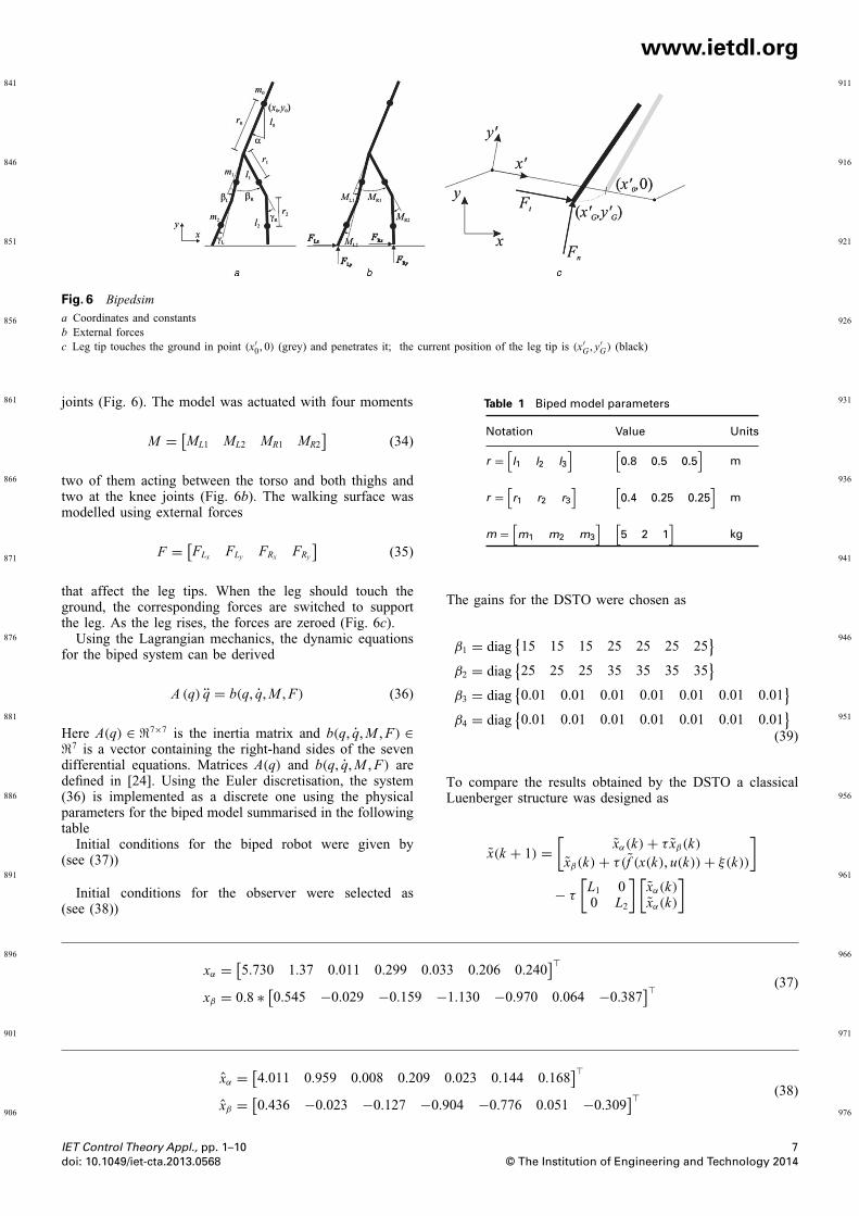
Initial conditions for the observer were selected as(see (38))

Table 1 Biped model parameters

Notation Value Units

r =[l1 l2 l3

] [0.8 0.5 0.5

]m

r =[r1 r2 r3

] [0.4 0.25 0.25

]m

m =[m1 m2 m3

] [5 2 1

]kg

The gains for the DSTO were chosen as

β1 = diag{15 15 15 25 25 25 25

}β2 = diag

{25 25 25 35 35 35 35

}β3 = diag

{0.01 0.01 0.01 0.01 0.01 0.01 0.01

}β4 = diag

{0.01 0.01 0.01 0.01 0.01 0.01 0.01

}(39)

To compare the results obtained by the DSTO a classicalLuenberger structure was designed as

x(k + 1) =[

xα(k) + τ xβ(k)

xβ(k) + τ(f (x(k), u(k)) + ξ(k))

]

− τ

[L1 00 L2

] [xα(k)xα(k)

]

xα = [5.730 1.37 0.011 0.299 0.033 0.206 0.240

]�

xβ = 0.8 ∗ [0.545 −0.029 −0.159 −1.130 −0.970 0.064 −0.387

]� (37)

xα = [4.011 0.959 0.008 0.209 0.023 0.144 0.168

]�

xβ = [0.436 −0.023 −0.127 −0.904 −0.776 0.051 −0.309

]� (38)


981

986

991

996

1001

1006

1011

1016

1021

1026

1031

1036

1041

1046

1051

1056

1061

1066

1071

1076

1081

1086

1091

1096

1101

1106

1111

1116

www.ietdl.org

Fig. 7 Position of selected states of the 24

Fig. 8 Velocity estimation of selected states of the biped simulator

with the following gains

L1 = 5 ∗ diag{15 15 15 25 25 25 25

}L2 = 5 ∗ diag

{25 25 25 35 35 35 35

} (40)

The trajectories for the DSTO and the Luenberger observerare depicted in Fig. 7. It can be seen how the trajectoriesof the DSTO converged closer to the real system trajecto-ries. The Luenberger state estimator did not converge to thereal states. In the same way, a similar comparison with thevelocities can be seen in Fig. 8. Again, a remark should be


1121

1126

1131

1136

1141

1146

1151

1156

1161

1166

1171

1176

1181

1186

1191

1196

1201

1206

1211

1216

1221

1226

1231

1236

1241

1246

1251

1256

www.ietdl.org

Fig. 9 Norm of the estimation error to compare a classicalLuenberger observer and the DSTO

done in the gains selection. The gains for the linear observerwere five times greater than the DSTO, this fact, implied afaster convergence into a zone for the Luenberger observerin similar way as it was claimed for the scalar case. How-ever, the error was bigger in the linear case when the systemwas in the steady state. It is important to note that only fourstates were plotted with the objective of keeping the lengthof the paper small enough. A complete analysis includingall the states of the biped model was done by means ofthe Euclidean norm of the error (Fig. 9). Moreover, fol-lowing the results presented in [24], where an animationof a biped was performed, in Fig. (10) this animation wasreprogrammed to present some clips of the animation withthe observer trajectories. In this figure, the mesh line areused to differentiate the left leg from the righ left of the

biped model. This animation was modified from the onepresented [24] in order to include a second biped that repre-sented the trajectories of the state estimator. In Fig. 10, thefirst biped corresponded to the DSTO and the second oneto the real system. In the instant t = τk = 0, the centre ofmass of the biped represented by the observer is ubicatedon the x-coordinates in x = 4.011 and the real system onx = 5.730. After some steps of time, the animation obtainedwith the DSTO reached the system. After t = τk = 1.75,the estimated biped reached the real biped animation. Thisconfirmed the complete reconstruction of the biped modelstates by the observer ones (21).

4 Conclusions

The Euler-like discretisation of the super-twisting algorithmwas successfully analysed in terms of Lyapunov stability.The behaviour of the DSTA has similar characteristics likeits continuous-time counterpart for small sampled periods.However, finite-time convergence cannot be proved withthis quadratic Lyapunov function. The convenient gains toensure the convergence of the DSTA were obtained bymeans of an LMI. A direct application of this new dis-crete structure is the problem of state estimation. Numericalresults showed how the observer can reach the real trajecto-ries of a n-degrees of freedom non-linear mechanical systemin a small period of time with better performance than theresults obtained by a Luenberger observer.

5 References

1 Spurgeon, S.: ‘Sliding mode observers: a survey’, Int. J. Syst. Sci.,2008, 39, (8), pp. 751–764

2 Atassi, A. N., Khalil, H.: ‘Separation results for the stabilization ofnonlinear systems using different high-gain observer design’, Syst.

Fig. 10 Clips taken from a biped simulation of model given in ( 36)


1261

1266

1271

1276

1281

1286

1291

1296

1301

1306

1311

1316

1321

1326

1331

1336

1341

1346

1351

1356

1361

1366

1371

1376

1381

1386

1391

1396

www.ietdl.org

Control Lett., 2000, 39, pp. 183–1913 Utkin, V.: ‘Sliding modes in control and optimization’ (Springer-

Verlag, 1992)Q44 Utkin, V.: ‘Sliding mode control in electro-mechanical systems’,

‘Automation and control engineering (CRC Press, 2009, 2nd edn.).5 Levant, A.: ‘Sliding order and sliding accuracy in sliding mode

control’, Int. J. Control, 1993, 58, (6), pp. 1247–12636 Levant, A.: ‘Principles of 2-sliding mode design’, Automatica, 2007,

43, (4), pp. 576–5867 Levant, A.: ‘Robust exact differentiation via sliding mode technique’,

Automatica, 1998, 34, (3), pp. 379–3848 Davila, J., Fridman, L., Levant, A.: ‘Second-order sliding-mode

observer for mechanical systems’, IEEE Trans. Autom. Control, 2005,50, (11), pp. 1785–1789

9 González, T., Moreno, J., Fridman, L.: ‘Variable gain super-twistingsliding mode control’, IEEE Trans. Autom. Control., 2012, 57, (8),pp. 2100–2105

10 Drakunov, S. V., Utkin, V.: ‘On discrete-time sliding mode’, Proc.IFAC Symp. Nonlinear Control Systems Design, 1989

11 Miloslavjevic, C.: ‘General conditions for the existence of a quasi-sliding mode on the switching hyperplane in discrete variable structuresystems’, Autom. Remote Control, 1985, 46, pp. 679–684

12 Sira-Ramirez, H.: ‘Nonlinear discrete variable structure systems inquasi-sliding mode’, Int. J. Control, 1991, 54, (5), pp. 1171–1187

13 Bartoszewicz, A.: ‘Discrete-time quasi-sliding mode control strate-gies’, IEEE Trans. Ind. Electron., 1998, 45, (4), pp. 633–637

14 Sarpturk, S. Z., Istefanopulos, Y., Kaynak, O.: ‘On the stability ofdiscrete-time sliding mode control systems’, IEEE Trans. Autom.Control, 1987, 32, (10), pp. 930–932

15 Chang, J. L.: ‘Robust discrete-time model reference sliding-mode con-troller design with state and disturbance estimation’, IEEE Trans. Ind.Electron., 2008, 55, pp. 4065–4074

16 Levant, A.: ‘Finite differences in homogeneous discontinuous control’,IEEE Trans. Autom. Control, 2007, 52, (7), pp. 1208–1217

17 Wang, B., Yu, X., Li, X.: ‘Zoh discretization effect on higher-ordersliding mode control systems’, IEEE Trans. Ind. Electron., 2008, 55,(11), pp. 4055–4064

18 Velovolu, K., Soh Y.C., Kao, W.: ‘Robust discrete-time nonlinearsliding mode state estimation of uncertain nonlinear systems’, Int. J.Robust Nonlinear Control, 2007, 17, pp. 803–828

19 Spurgeon, S. K.; ‘Hyperplane design techniques for discrete-timevariable structure control systems’, Int. J. Control, 1992, 55, (2),pp. 445–456

20 Koshkouei, J., Zinover, A. S.: ‘Sliding mode state observers for SISOlinear discrete systems’, UKACC Int. Conf. Control, 1996

21 Bartolini, G., Pisano, A., Usai, E.: ‘Digital second-order sliding modecontrol for uncertain nonlinear systems’, Automatica, 2001, 37, (9),pp. 1371–1377

22 Salgado, I., Moreno, A., Chairez, I.: ‘Sampled output based continuoussecond-order sliding mode observer’, Workshop on Variable StructureSystems, 2010

23 Davila, J., Fridman, L., Poznyak, A.: ‘Observation and identification ofmechanical systems via second-order sliding modes’, Int. J. Control,2006, 79, (10), pp. 1251–1262

24 Havisto, H., Hyötyniemi, ‘Simulation tool of a biped walking robotmodel’, Technical Report, Control Engineering Laboratory, HelsinkiUniversity of Technology, 2004

25 Poznyak, A.: ‘Advanced mathematical tools for automatic controlengineers: volume 1: Deterministic systems’ (Elsevier Science, 2008)

6 Appendix

Proof: (Proof of Theorem 1) Consider the following functionlike a candidate Lyapunov one

V (x) := ‖x‖2P (41)

Let �V (k) := V (k + 1) − V (k) then

�V (k) = x�(k + 1)Px(k + 1) − x�(k)Px(k) (42)

Substituting (4) into (42) the terms �V (k) becomes

�V (k) = x�(k)(A�PA − P)x(k)+2x�(k)A�PB(k)

× sign(x1(k)) + B�(k)PB(k) (43)

Using the so-called lambda inequality [25] X �Y + Y �X ≤X ��−1X + Y ��Y for 2x�(k)A�PB(k)sign (x1(k)) the fol-lowing result was obtained

2x�(k)A�PB(k)sign(x1(k))

≤ x�(k)A�P�−1PAx(k) + B�(k)�B(k)(44)

Equation (43) turns in

�V (k) ≤ x�(k)(A�(P + P�P)A − (1 − �)P)x(k)

+ B�(k)(�−1+P)B(k) − �V (k)(45)

Then, expanding the term B�(k)ZB(k) with Z := (�−1 + P),one has

B�(k)ZB(k) = δ1|x1(k)| + δ2|x1(k)|1/2 + δ3

δ1 := τ 2k21 z11, δ2 := τ 2k1k2z12, δ3 := τ 2k2

2 z22

(46)

Using again the lambda inequality in the term containingδ2 and if there exists a matrix Q = Q� > 0 solution forthe LMI given by A�(P + P�P)A − (1 − �)P = −Q, then�V (k) becomes into (for any ω1 ∈ R

+)

�V (k) ≤ −‖x(k)‖2Q + δ1|x1(k)| + δ2−�V

δ1 := δ1 + τ 4k21 k2

2 z212ω1,

δ2 := k22 τ

2(τ 2k2

1 z212ω

−11 +z22)

(47)

Following the previous result

�V ≤ −‖x(k)‖2Q + δ1‖QQ−1x(k)‖ − αV + δ2

= −(

‖Q1/2x(k)‖ − 1

2δ1‖Q−1‖

)T

×(

‖Q1/2x(k)‖ − 1

2δ1‖Q−1‖

)

− αV + δ2 + 1

4δ2

1‖Q−1‖2

(48)

then

�V (k)≤ −�V (k) + c (49)

with c := δ2 + 14 δ

21‖Q−1‖2.

V (k + 1) ≤ − (1 − �) V (k) + c (50)

The last equation is well defined as a discrete linear one andthe solution is given by

V (k + 1) ≤ (1 − �)kV (0) +k∑

i=1

(1 − γx)i−1 c (51)

If the upper limit when k goes to infinity is considered, onehas

limk→∞V (k) ≤ c

1 − �(52)

and the radius of the region of convergence of the DSTA isdefined as

r ≤ c

1 − �(53)

This result completes the proof. �


1401

1406

1411

1416

1421

1426

1431

1436

1441

1446

1451

1456

1461

1466

1471

1476

1481

1486

1491

1496

1501

1506

1511

1516

1521

1526

1531

1536

www.ietdl.org

CTA20130568

Author Queries

Iván Salgado, I. Chairez, Bijnan Bandyopadhyay, Leonid Fridman and Oscar Camacho

Q1 Please provide the initial of author named Chairez.

Q2 Please provide main caption for figure 3.

Q3 Please cite table 1 in the text cited in text.

Q4 Please provide editor name in ref. [4].

Documents

ISSN 1751-8644 Discrete-time non-linear state observer