ISO/TC 131/WG 4 N 566 ISO/CD TR 16194nfpahub.com/wp-content/uploads/2015/10/16194-dtr-For_US_input.pdf · reproduction of working drafts or committee drafts in any form for use by

© ISO 2014 All rights reserved

C:\Users\drockhill\Desktop\131-wg4-TR-16194-n563-draft for direct publication.doc Basic template BASICEN3 2002-06-01

Reference number of working document: ISO/TC 131/WG 4 N 566 Date: 2015-09-18

Reference number of document: ISO/CD TR 16194

Committee identification: ISO/TC 131/WG 4

Secretariat: DIN

Pneumatic fluid power Assessment of component reliability by accelerated life testing General guidelines and procedures

Élément introductif Élément principal Partie n: Titre de la partie

Warning

This document is not an ISO International Standard. It is distributed for review and comment. It is subject to change without notice and may not be referred to as an International Standard.

Recipients of this draft are invited to submit, with their comments, notification of any relevant patent rights of which they are aware and to provide supporting documentation.

Document type: Technical Report Document subtype: if applicable Document stage: (20) Preparatory Document language: E

ISO/TC 131/WG 4 N 563 ISO/CD TR 16194 2015-09-18

ii © ISO 2014 All rights reserved

Copyright notice

This ISO document is a working draft or committee draft and is copyright-protected by ISO. While the reproduction of working drafts or committee drafts in any form for use by participants in the ISO standards development process is permitted without prior permission from ISO, neither this document nor any extract from it may be reproduced, stored or transmitted in any form for any other purpose without prior written permission from ISO.

Requests for permission to reproduce this document for the purpose of selling it should be addressed

[Indicate : the full address telephone number fax number telex number and electronic mail address

as appropriate, of the Copyright Manager of the ISO member body responsible for the secretariat of the TC or SC within the framework of which the draft has been prepared]

Reproduction for sales purposes may be subject to royalty payments or a licensing agreement.

Violators may be prosecuted.


© ISO 2014 All rights reserved iii

Contents Page

Foreword .............................................................................................................................................................. v

Introduction ........................................................................................................................................................ vi

1 Scope ...................................................................................................................................................... 1

2 Normative references ............................................................................................................................ 1

3 Terms and definitions ........................................................................................................................... 2

4 Symbols and units ................................................................................................................................. 3

5 Concepts of reliability and accelerated life testing ............................................................................ 3

6 Failure mechanism and mode .............................................................................................................. 4

7 Strategy of conducting accelerated life testing.................................................................................. 4

8 Design of accelerated life testing ........................................................................................................ 5 8.1 Normal use conditions .......................................................................................................................... 5 8.2 Preliminary tests .................................................................................................................................... 6 8.3 Levels of accelerated stress ................................................................................................................. 7 8.4 Sample size ............................................................................................................................................ 8 8.5 Data observation and measurement .................................................................................................... 8 8.6 Types of stress loading ......................................................................................................................... 8

9 End of test .............................................................................................................................................. 9 9.1 Minimum number of failures required ................................................................................................. 9 9.2 Termination cycle count ....................................................................................................................... 9 9.3 Suspended or censored test units ....................................................................................................... 9

10 Statistical analysis ................................................................................................................................. 9 10.1 Analysis of failure data ......................................................................................................................... 9 10.2 Life distribution .................................................................................................................................... 10 10.3 Accelerated life testing model ............................................................................................................ 11 10.4 Data analysis and parameter estimation ........................................................................................... 11

11 Reliability characteristics from the test data .................................................................................... 11

12 Test report ............................................................................................................................................ 12

Annex A (normative) Determining stress levels when stress is time-dependent ..................................... 13

Annex B (informative) Life-stress relationship models ............................................................................... 17 B.1 Acceleration factor .............................................................................................................................. 17 B.2 Arrhenius life-stress model ................................................................................................................ 17 B.3 Inverse power law life-stress model .................................................................................................. 18 B.4 Eyring life-stress model ...................................................................................................................... 19 B.5 Temperature-humidity combination model ....................................................................................... 21 B.6 Temperature-nonthermal combination model .................................................................................. 22 B.7 General log-linear model ..................................................................................................................... 23

Annex C (informative) Validation and verification of accelerated life test ................................................ 26

Annex D (informative) Calculation procedures for censored data ............................................................. 28

Annex E (informative) Examples of using accelerated life testing in industrial applications ................. 31 E.1 Pneumatic cylinder .............................................................................................................................. 31 E.2 Flexible hose ........................................................................................................................................ 32

Annex F (informative) Palmgren- ............................................................................................... 33


iv © ISO 2014 All rights reserved

Annex G (informative) G.1 G.2 Bas 6 G.3 G.4 G.5

Bibliography ...................................................................................................................................................... 48


© ISO 2014 All rights reserved v

Foreword

ISO (the International Organization for Standardization) is a worldwide federation of national standards bodies (ISO member bodies). The work of preparing International Standards is normally carried out through ISO technical committees. Each member body interested in a subject for which a technical committee has been established has the right to be represented on that committee. International organizations, governmental and non-governmental, in liaison with ISO, also take part in the work. ISO collaborates closely with the International Electrotechnical Commission (IEC) on all matters of electrotechnical standardization.

International Standards are drafted in accordance with the rules given in the ISO/IEC Directives, Part 2.

The main task of technical committees is to prepare International Standards. Draft International Standards adopted by the technical committees are circulated to the member bodies for voting. Publication as an International Standard requires approval by at least 75 % of the member bodies casting a vote.

Attention is drawn to the possibility that some of the elements of this document may be the subject of patent rights. ISO shall not be held responsible for identifying any or all such patent rights.

ISO TR 16194 was prepared by Technical Committee ISO/TC 131, Fluid power systems.


vi © ISO 2014 All rights reserved

Introduction

This ISO TR is being released to document progress that the working group has developed for accelerated testing. It is a new method with which the working group members have very little experience, but has been used by institutional laboratories and taught at academic levels.

Some experimentation on air cylinders has been done at the Korean Institute of Machinery and Materials (KIMM), but the application to pneumatic components in general has not been evaluated. This ISO TR is offered to the members as a reference and model procedure, in order that they may develop experience with its use in their own laboratories.

WORKING DRAFT ISOTC 131/WG 4 N 563 ISO/CD TR 16194 2015-07-08

© ISO 2014 All rights reserved 1

Pneumatic fluid power Assessment of component reliability by accelerated life testing General guidelines and procedures

1 Scope

This Technical Report provides general procedures for assessing the reliability of pneumatic fluid power components using accelerated life testing and the method for reporting the results. These procedures apply to directional control valves, cylinders with piston rods, pressure regulators, and accessory devices the same components covered by the ISO 19973 series of standards.

This Technical Report does not provide specific procedures for accelerated lift testing of components. Instead, it explains the variability among methods and provides guidelines for developing an accelerated test method.

The methods specified in this Technical Report apply to the first failure, without repairs.

2 Normative references

The following referenced documents are indispensable for the application of this document. For dated references, only the edition cited applies. For undated references, the latest edition of the referenced document (including any amendments) applies.

ISO 5598, Fluid power systems and components Vocabulary

ISO 19973-1, Pneumatic fluid power Assessment of component reliability by testing Part 1: General procedures

ISO 19973-2, Pneumatic fluid power Assessment of component reliability by testing Part 2: Directional control valves

ISO 19973-3, Pneumatic fluid power Assessment of component reliability by testing Part 3: Cylinders with piston rod

ISO 19973-4, Pneumatic fluid power Assessment of component reliability by testing Part 4: Pressure regulators

ISO 19973-5, Pneumatic fluid power Assessment of component reliability by testing Part 5: Non-return valves, shuttle valves, dual pressure valves, one-way adjustable flow control valves, quick-exhaust valves

ISO 80000-1, Quantities and units Part 1: General


2 © ISO 2014 All rights reserved

3 Terms and definitions

For the purposes of this document, the terms and definitions given in ISO 5598, ISO 19973-1 and the following apply.

3.1 Bx life life of a component or assembly that has not been altered since its production, where its reliability is

( %; or the time at which ( % of the population has survived

NOTE The cumulative failure fraction is x %. For example, if x = 10, the B10 life has a cumulative failure probability of 10 %.

3.2 acceleration factor (AF) ratio between the life at the normal use stress level and the life at the accelerated stress level

3.3 accelerated life test (ALT) process in which a component is forced to fail more quickly that it would have under normal use conditions

3.4 destruct limit

is no longer within specification or the component is damaged and cannot recover when the stress is reduced

NOTE Destruct limits are classified as a lower destruct limit and upper destruct limit.

3.5 failure mechanism physical or chemical process that produces instantaneous or cumulative damage to the materials from which the component is made

3.6 failure mode manifestation of the failure mechanism resulting from component failure or degradation

NOTE The failure mode is the symptom of the aggressive activity of the failure mechanism in tof weakness, where stress exceeds strength.

3.7 failure rate, frequency at which a failure occurs instantaneously at time t, given that no failure has occurred before t

3.8 highly accelerated life test (HALT) process in which components are subjected to accelerated environments to find weaknesses in the design and/or manufacturing process

NOTE The primary accelerated environments include pressure and heat.

3.9 model for accelerated life testing model that consists of a life distribution (for example, Weibull, Lognormal, Exponential, etc.) that represents the scatter in component life and a relationship (for example, Arrhenius, Eyring, Inverse Power Law, etc.) between life and stress



3.10 normal use conditions test conditions at which a component is commonly used in the field, which may be less strenuous than rated conditions

3.11 termination cycle count number of cycles on a test item when it reaches a threshold level for the first time

4 Symbols and units

4.1 The symbols used in this International Standard are given in Table 1.

Table 1 Symbols

Symbol a Definition

B10 Time at which 10 % of the population will fail

Scale parameter (characteristic life) of the Weibull distribution

F(t) Probability of failure of a component up to time t

Shape parameter (slope) of the Weibull distribution

R(t) Reliability of a component at time t; R(t) = 1 F(t)

(t) Failures per unit time

a Other symbols could be used in other documents and software.

4.2 Units of measurements should be in accordance with ISO 80000-1.

5 Concepts of reliability and accelerated life testing

Reliability is the probability (a percentage) that a component will not fail (for example, exceed the threshold level or experience catastrophic failure) for a specified interval of time or number of cycles when it operates under stated conditions. This reliability may be assessed by test methods described in the ISO 19973 series.

Generally, reliability analysis involves analyzing time to failure of a component obtained under normal use conditions in order to quantify its life characteristics. Obtaining such life data is often difficult.

The reasons for this difficulty can include the typically long life times of components, the small time period between design and product release, and the necessity for testing components under normal use conditions. Given this difficulty and the need to observe failures of components to better understand their life characteristics, procedures have been devised to accelerate their failures by overstress, thus forcing components to fail more quickly than they would under normal use conditions. The term accelerated life testing (ALT) is used to describe such procedures.

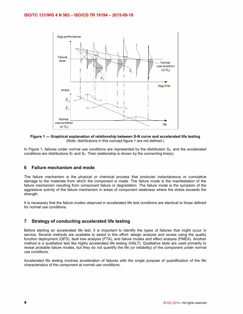
However, a relationship between the reliability of a component determined by ALT, and its reliability at normal use conditions, is necessary. This can be assessed by extrapolating the test results obtained from an accelerated life testing and comparing it to that obtained from testing at normal use conditions. Figure 1 shows the graphical concept for this relationship.



Figure 1 Graphical explanation of relationship between S-N curve and accelerated life testing (Note: distributions in this concept figure 1 are not defined.)

In Figure 1, failures under normal use conditions are represented by the distribution S3, and the accelerated conditions are distributions S1 and S2. Their relationship is shown by the connecting line(s).

6 Failure mechanism and mode

The failure mechanism is the physical or chemical process that produces instantaneous or cumulative damage to the materials from which the component is made. The failure mode is the manifestation of the failure mechanism resulting from component failure or degradation. The failure mode is the symptom of the aggressive activity of the failure mechanism in areas of component weakness where the stress exceeds the strength.

It is necessary that the failure modes observed in accelerated life test conditions are identical to those defined for normal use conditions.

7 Strategy of conducting accelerated life testing

Before starting an accelerated life test, it is important to identify the types of failures that might occur in service. Several methods are available to assist in this effort: design analysis and review using the quality function deployment (QFD), fault tree analysis (FTA), and failure modes and effect analysis (FMEA). Another method is a qualitative test like highly accelerated life testing (HALT). Qualitative tests are used primarily to reveal probable failure modes, but they do not quantify the life (or reliability) of the component under normal use conditions.

Accelerated life testing involves acceleration of failures with the single purpose of quantification of the life characteristics of the component at normal use conditions.



Therefore, accelerated life testing can be divided into two areas: qualitative accelerated testing (HALT) and quantitative accelerated life testing. In qualitative accelerated testing, the objective is to identify failures and failure modes without attconditions. In quantitative accelerated life testing, the objective is predicting the life of the component (life characteristics such as MTTF, B10 life, etc.) at normal use conditions from data obtained in an accelerated life test.

The strategy for effectively conducting an accelerated life testing program includes the following:

establishing a stress level that can be referred to as normal use conditions;

determining the stress levels to use for accelerated testing;

determining the number of components to be tested at each stress level.

8 Design of accelerated life testing

8.1 Normal use conditions

characteristics, for example, pressure, temperature, voltage, duty cycle, lubrication requirements, etc. However, these ratings often represent a maximum condition that is above commonly used conditions. Therefore, a definition for normal use conditions needs to be established from these characteristics before starting an accelerated test. An example definition for a pneumatic valve is shown in Table 2.

Table 2 Definition of normal use conditions for a pneumatic valve

Characteristic Typical rating value Common use

application value

Proposed normal use value

for testing

Pressure 100 kPa (10 bar) 63 kPa (6,3 bar) 63 kPa (6,3 bar)

Temperature 50 C 25 C 25 C

Voltage 24 VDC 24 VDC 24 VDC

Duty cycle Continuous On-off varies 10 % on / 90 % off

Lubrication Sometimes required Sometimes applied Not used

Air dryness Dew point < 0 C Dew point C Dew point = 10 C

It is necessary to define this normal use conditions before starting an ALT program.



8.2 Preliminary tests

It is also necessary to determine the highest stress to be tested that will not result in failure modes different than those that occur under normal use conditions. Typically, these stresses or limits are unknown, so qualitative tests (HALT) with small sample sizes can be performed in order to determine the appropriate stress levels for use in the accelerated life test. Design of Experiments (DOE) methodology is a useful technique at this step.

The following steps can be taken to determine three stress levels:

a) Propose the highest possible stress that might yield failure in less than 1 day of testing (approximately).

b) Reduce this stress level to 90% of that value and test at least two test units to failure at this stress level, using the test procedures of one of the parts of the ISO 19973 series (modified for the conditions of the stress level).

c) Examine the failure mode to determine if it is the same type of failure as would be experienced under normal use conditions. If it is not, reduce the level of stress and repeat steps b) and c) until failures are the same as would be experienced under normal use conditions. Identify this as stress level S1.

d) Reduce the stress level by another 10% to 20% from step b) and test at least two more test units to failure. Again, examine the failure mode to determine if it is the same type of failure as would be experienced under normal use conditions. If it is not, modify the stress conditions and repeat the test. Identify this as stress level S2. See Figure 2.

e) Identify the third, lowest stress level S3 that will result in failures within project timing constraints. This third level of stress is identified by extrapolating from the previous pairs of failures as shown in Figure 2. As an alternative, S2 can be estimated by using an average value of S1 and S3, so that S3 = 2S2 S1.

f) Test at least two more test units to failure at this third level of stress S3. Again, examine the failure mode to determine if it is the same type of failure as would be experienced under normal use conditions. If it is not, modify the stress conditions and repeat the test.



Figure 2 Graphical explanation of determining stress levels during preliminary tests

These preliminary tests may need to be conducted several times before the necessary stress levels are determined.

8.3 Levels of accelerated stress

The levels of stress identified from 8.2 are used to conduct a series of accelerated tests on randomly selected test units, in accordance with one of the parts of ISO 19973. Generally, these stress levels will fall outside of

tantly examine the types of failures obtained to be sure they are the same as those experienced at normal use conditions. If they are not, the test units would be designated as suspensions, or the test conditions should be modified and the testing restarted.

Conduct the tests at each of the selected stress levels. It is also helpful to conduct at least one test at a stress level that is as close as possible to the normal use conditions.

At the higher levels of stress in an accelerated test, the required test duration decreases, and the uncertainty in the extrapolation increases. Confidence intervals provide a measure of the uncertainty in extrapolation.

The most common stresses for pneumatic fluid power components are pressure and temperature. Testing can be conducted either at one set of stress conditions on a sample lot, or two stresses on different sample lots.

Temperature of the process air used to test components should be heated (or cooled) to approximately equal the environmental test temperature.



When conducting an accelerated life test, arrangements should be made to ensure that the failures of the components are independent of each other (e.g. failures due to temperature should not influence the failures due to pressure).

8.4 Sample size

Ideally, at least seven test units should be subjected to each stress level for the accelerated life test. However, the number of test units allocated to each stress level should be inversely proportional to the level of applied stress; that is, more test units should be subjected to lower stress levels than to higher stress levels because of the higher proportion of failures expected at the higher stress levels. A good ratio for the number of test units among the stress levels, from highest to lowest, is 1:2:4. If test units are expensive, four test units each at stress levels S1 and S2 would be tested; and five or more test units would be tested at stress level S3. As an option, the number of test units could be two if time is limited, but the estimation uncertainty at the normal use condition will increase.

8.5 Data observation and measurement

No repairs are made to the test units during accelerated life testing.

The test operator should determine the intervals between measurements to obtain data during accelerated life testing. Short intervals between measurements give better statistical results and should be conducted during testing at the high stress level. At the low stress levels, longer intervals between measurements are adequate.

8.6 Types of stress loading

There are two possible stress loading schemes: loading in which the stress is time-independent (where the stress does not vary over time), and loading in which the stress is time-dependent (where the stress does vary over time). This Technical Report uses constant time-independent stress loading, which is the most common type used in an accelerated life test; see Figure 3. However, non-constant stress loads, such as step stress, cycling stress, random stress, etc., can be used. These types of loads are classified according to their dependence on time and are described in Annex A. The method specified in Annex A should be used where a time-dependent analysis is required.

TimeTimeTime

Figure 3 Constant stress model



Time-independent stress loading has many advantages over time-dependent stress loading. Specifically;

most components are assumed to operate at a constant stress under normal use conditions;

it is far easier to run a constant stress test;

it is far easier to quantify a constant stress test;

models for data analysis are widely publicized and are empirically verified; and

extrapolation from a well-executed constant stress test is more accurate than extrapolation from a time-dependent stress test.

9 End of test

9.1 Minimum number of failures required

In order to generate confidence levels, at least four test units should have failed (which includes their reaching a threshold level) at each stress level.

9.2 Termination cycle count

When a test unit fails between consecutive observations, the data collected is referred to as left-censored or interval data. In this case, both the last cycle count at which the test unit was operating properly and the cycle count at which the test unit was observed to have failed, should be recorded. This data should be processed in accordance with 10.2 of ISO 19973-1.

9.3 Suspended or censored test units

Individual test units on which testing was stopped before failure occurred are known as suspensions. Some examples of suspensions include:

the test unit needed to be disassembled for inspection;

the test unit experienced an incorrect failure mode;

the test unit was accidentally damaged from a source not related to the test.

Because these test units had achieved a number of cycles before the point of suspension, the data has a positive influence on the calculation of the statistical parameters. However, they can not be returned to the testing program.

If the minimum number of failures has been reached, but some test units have not failed (reached a threshold level), the test may be stopped. The remaining test units are designated as censored.

Data from suspended test units is considered the same as data from censored test units. The method specified in Annex D should be used to calculate the statistical parameters for these types of data

10 Statistical analysis

10.1 Analysis of failure data

The failure data from testing at all stress levels should be analyzed in accordance with 10.2, 10.3 and 10.4.



10.2 Life distribution

Select an initial life distribution (it can be changed later, if necessary). For pneumatic components, the Weibull distribution is commonly used, and its scale parameter, , is selected to be the life characteristic that is

stress-dependent; while the slope

Plot the raw data from all stress levels on one graph and obtain a best fit straight line to the data from each stress level (see Figure 4 vel are not parallel, consider a compromise slope for each set of stress levels (see Figure 5). A judgment is necessary as to whether the compromise introduces too much of an error, and if this is judged to be the case, the testing program should be restarted weach stress level.

Figure 4 Best fit slope lies to raw data

Figure 5 Compromised equal slope lines



The resulting distribution should be verified by using a probability plot as described in Annex C. If the lines fitted from the plotted data at each accelerating stress level are parallel, it implies that the failure mechanism at each stress level is the same, and the selected stress levels for the accelerated testing are appropriate.

10.3 Accelerated life testing model

Select or create a model of accelerated life testing that describes a life characteristic of the distribution from one stress level to another; this is also called a life-stress relationship model. Examples of these models include the Arrhenius, Eyring, Inverse Power Law, etc., and are described in Annex B.

10.4 Data analysis and parameter estimation

Using the selected life-stress relationship model, estimate the parameters of the life-stress distribution using either a graphical method, a least squares method, or the maximum likelihood estimation (MLE) method. An example using the Arrhenius model with a graphical estimation method is shown in Figure 6.

Figure 6 Arrhenius plot of data from Figure 5

In Figure 6, the individual dots are the raw data points, and the connecting line joins the characteristic life

from each stress level. The example curves in Figures 4, 5 and 6 used a Weibull distribution.

NOTE Commercial software may be helpful in developing all of these plots.

The acceleration factor (AF) can now be determined from a simple proportion of lives at the normal use life to those at any accelerated condition. Methods of calculating acceleration factors are given in Annex B of this International Standard.

11 Reliability characteristics from the test data

11.1 To improve the interpretation of the calculation results, the failure mode for each test unit should be recorded.



11.2 Calculations should be made from the test data at each stress level to determine

characteristic life ;

Weibull shape parameter , slope of the straight line in the Weibull plot;

the mean life, which provides a measure of the average time of operation to failure;

BX life, which is the time by which X% of the components will fail; and

the confidence intervals of the BX life at the 95% confidence level using Fisher information matrix,

11.3 Calculations should be made from the life-stress analysis to determine

model parameters and acceleration factor, and

BX life and confidence intervals of Bx life at the normal use conditions.

12 Test report

The test report should include at least the following data:

a) the number of this Technical Report including the component-specific part number;

b) date of the test report;

c) component description (manufacturer, type designation, series number, date code);

d) sample size;

e) test conditions (types of stress, number of stress levels, stress loading, etc.);

f) threshold levels;

g) shape parameter ( );

h) types of failures for each test unit;

i) B10 life and confidence intervals of B10 life at 95% confidence level under normal use conditions;

j) characteristic life under normal use conditions;

k) number of failures considered;

l) method used to calculate the Weibull data (Maximum likelihood, etc.);

m) model for accelerated life testing (Arrhenius-Weibull, Eyring-Weibull, Inverse power law-Weibull, etc.);

n) acceleration factor;

o) parameters of the selected acceleration model;

p) other remarks, as necessary.



Annex A

Determining stress levels when stress is time-dependent

When the stress is time-dependent, the component is subjected to a stress level that varies with time. Components subjected to time-dependent stress loadings will yield failures more quickly, and models that fit them are valuable methods of accelerated life testing.

The step-stress model and the related ramp-stress model are typical cases of time-dependent stress tests. In these cases, the stress load remains constant for a period of time and then is stepped / ramped into a different stress level where it remains constant for another time interval until it is stepped / ramped again. There are numerous variations of this concept as shown in figures A.1 to A.4:

TimeTimeTime

TimeTimeTime

Figure A.1 Step stress model Figure A.2 Ramp stress model

TimeTimeTime

TimeTimeTime

Figure A.3 Increasing stress model Figure A.4 Complete time-dependent stress model



There are some cases where the stress in a field operating condition is variable. In that case, the following steps are helpful to process the accelerated life test:

a) First, identify the field operating condition for a related component. The result using histogram is shown in Figure A.5.

b) Calculate equivalent load needed for accelerated life testing using Palmgren-Figure A.6 represents the equivalent load for the resulting accelerated life test.

Figure A.5 Field operating condition Figure A.6 Equivalent damage effect calculation

c) Decide upon a step-stress loading method to determine a destruct limit and yield point for the accelerated life testing. Figure A.7 shows step-stress loading method.

d) Determine the appropriate stress range using destruct limit, operating limit (or elastic limit), and specification limit (proportional limit) of a strain-stress curve as shown in Figure A.8.

e) Find the accelerated stress level using an accelerated life test curve as shown in Figure A.9. In the field of mechanical engineering, overstress levels commonly used in industry are 120 %, 133 %, and 150 %.

f) Determine the stress levels using a step by step process (see Figure A.10) and the procedure given in 8.2. Accelerated life testing at the three accelerating stress levels can then be performed.



Figure A.7 Step-stress loading method Figure A.8 Strain-stress curve

Figure A.9 Accelerated life test curve Figure A.10 Decision method of stress levels

g) Before estimating the reliability characteristics, check on the validation of accelerated test using

probability plot in Figure A.11. If the fitted lines of the plotted data at each accelerating stress levels are parallel, it means that assumed lifetime distribution is appropriate and the accelerating stress is effective.



h) Check the error between the estimates of the considered model and real test results. First, check that the shape parameters acquired from the considered model, and tested results in normal use conditions, are the same. Second, check if the scale parameter of the considered model resides in the confidence intervals of scale parameter from the test results. Finally, if the scale parameter of the considered model is within the confidence intervals, it could be judged that both the characteristic life of the considered model and test result are not statistically different. Figure A.12 shows the graphical explanation of the error between estimate of the considered model and test result.

Figure A.11 Validation and verification of accelerated test

Figure A.12 Graphical explanation of the error between test estimate of the considered model

and test result



Annex B

Life-stress relationship models

B.1 Acceleration factor

The acceleration factor is a unitless number that relates a com life at an accelerated stress level to the life at the normal use stress level. It is defined by;

A

U

L

LAF (B.1)

where

UL is the life at the normal use stress level

AL is the life at the accelerated stress level

As it can be seen in equation (B.1), the acceleration factor depends on the life-stress model and is thus a function of stress.

B.2 Arrhenius life-stress model

The Arrhenius life-stress model (or relationship) is probably the most common life-stress model utilized in accelerated life testing. It has been widely used when the stimulus or accelerated stress is thermal (i.e. temperature).

The Arrhenius life-stress model is formulated by assuming that life is proportional to the inverse reaction rate of the process, thus the Arrhenius life-stress model is given by;

V

B

(B.2)

where

L is the quantifiable life measure (mean life, characteristic life, median life, BX life, etc.)

V is the stress level (temperature values in degrees Kelvin)

C and B are the model parameter (C>0, B>0)

Because the Arrhenius is a physics-based model derived for temperature dependence, it is strongly recommended that the model be used for temperature-accelerated tests.

The Arrhenius model is linearized by taking the natural logarithm of both sides in equation (B.2).

(B.3)

Depending on the application (and where the stress is exclusively thermal), the parameter B can be replaced by;



(B.4)

The activation energy must be known a priori. If the activation energy is known, then only model parameter C remains. Because in most real-life situations this is rarely the case, all subsequent formulations will assume that this activation energy is unknown and treat B as one of the model parameters. B is a measure of the effect that the stress (i.e. temperature) has on the life. The larger the value of B, the higher the dependency of the life on the specific stress.

Most practitioners use the term acceleration factor to refer to the ratio of the life (or acceleration characteristic) between the normal use level and a higher test stress level. For the Arrhenius model, acceleration factor is;

AU

A

UV

B

V

B

V

B

V

B

dAccelerate

USE e

eC

eC

L

LAF . (B.5)

The probability density function for 2-parameter Weibull distribution is given by;

t1

(B.6)

The scale parameter (or characteristic life) of the Weibull distribution is . The Arrhenius-Weibull model probability density function at a stress level V can then be obtained by setting = L(V) in equation (B.2);

(B.7)

and substituting for in equation (B.6);

V

B

eC

t

V

B

V

Be

eC

t

eC

Vtf

1

);( (B.8)

The mean time to failure (MTTF) of the Arrhenius-Weibull model is given by;

(B.9)

where is the gamma function.

The Arrhenius-Weibull reliability function at stress level V is given by;

V

B

eC

t

eVtR );( (B.10)

B.3 Inverse power law life-stress model

The inverse power law (IPL) model is commonly used for non-thermal accelerated stresses and is given by;



n (B.11)

where


V is the stress level

K and n are model parameters (K>0, n>0)

The inverse power law appears as a straight line when plotted on a log-log paper. The equation of the line is given by;

(B.12)

The parameter in the inverse power model is a measure of the effect of the stress on the life, i.e., the larger the value of n, the greater the effect of the stress. A value of n approaching 0 indicates small effect of the stress on the life, with no effect (constant life with stress) when n = 0.

For the inverse power law model, the acceleration factor is given by;

n

U

A

nA

nU

dAccelerate

USE

V

V

KV

KV

L

LAF

1

1

(B.13)

The inverse power law Weibull model can be derived by setting = L(V), yielding the following IPL-Weibull probability density function at stress level V;

(B.14)

The mean time to failure (MTTF) of the IPL-Weibull model is given by;

(B.15)

The IPL-Weibull reliability function at stress level V is given by;

(B.16)

B.4 Eyring life-stress model

The Eyring life-stress model was formulated from quantum mechanics principles and is most often used when thermal stress (temperature) is the acceleration variable. However, the Eyring model is also often used for stress variables other than temperature, such as humidity. The model is given by;

(B.17)

where




V is the stress level

A and B are model parameters

For the Eyring model the acceleration factor is given by;

AU

A

u

VVB

U

A

V

BA

A

V

BA

u

dAccelerate

USE eV

V

eV

eV

L

LAF

11

1

1

(B.18)

The Eyring-Weibull model can be derived by setting = L(V), yielding the following Eyring-Weibull probability density function at stress level V;

V

BA

eVt

V

BA

V

BA

eeVteVVtf

1

);( (B.19)

The mean time to failure (MTTF) of the Eyring-Weibull model is given by;

(B.20)

The Eyrin-Weibull reliability function at stress level V is given by;

V

BA

etV

(B.21)



B.5 Temperature-humidity combination model

The temperature-humidity (T-H) combination model, a variation of the Eyring relationship, has been proposed for predicting the life at normal use conditions when temperature and humidity are the accelerated stresses in a test. This combination model is given by;

(B.22)

where


V is the temperature

U is the relative humidity (decimal or percentage)

is a model parameter

B is a model parameter (also known as the activation energy for humidity)

A is a constant and model parameter

The T-H combination model can be linearized and plotted on a life vs. stress plot. The model is linearized by taking the natural logarithm of both sides in equation (B.22), or;

(B.23)

Depending on which type of stress is kept constant, it can be seen from equation (B.23) that either the parameter or the parameter b is the slope of the resulting line. If, for example, the humidity is kept constant,

then is the slope of the life line in a life vs. temperature plot. The steeper the slope, the more the

In other words, is a measure of the effect that

temperature has on the life, and b is a measure of the effect that relative humidity has on the life. The larger the value of , the more the life depends on the effect of temperature. Similarly, the larger the value of b, the

more the life depends on the effect of relative humidity.

The acceleration factor for the T-H model is given by;

AUAU

AA

UUUU

bVV

U

b

V

U

b

V

dAccelerate

USE e

eA

eA

L

LAF

1111

(B.24)

By setting = L(V;U) as given in equation (B.22), the T-H Weibull model's probability density function at stress level V and U is given by

U

b

VeA

t

U

b

VU

b

V eeA

te

AUVtf

1

);;( (B.25)



The mean time to failure (MTTF) of the T-H Weibull model is given by;

(B.26)

The T-H Weibull reliability function at stress level V and U is given by;

U

b

VeA

t

(B.27)

B.6 Temperature-nonthermal combination model

When temperature and a second non-thermal stress (e.g. voltage or pressure) are the accelerated stresses of a test, then the Arrhenius and the inverse power law relationships can be combined to yield the temperature-nonthermal (T-NT) combination model. This model is given by;

V

Bn eU

CUVL );( (B.28)

where


V is the temperature (in degrees K)

U is the non-thermal stress (i.e., voltage, vibration, pressure, etc.)

B, C and n are model parameters

The T-NT combination model can be linearized and plotted on a life vs. stress plot. The model is linearized by taking the natural logarithm of both sides in equation (B.28) or;

(B.29)

Because the life is now a function of two stresses, a life vs. stress plot can only be obtained by keeping one of the two stresses constant and varying the other.

The acceleration factor for the T-NT model is given by;

AU

A

U

VVBn

U

A

V

B

nA

V

B

nU

dAccelerate

USE eU

U

eU

C

eU

C

L

LAF

11

(B.30)



By setting = L(V, U) as given in equation (B.28), the T-NT Weibull model's probability density function at stress levels V and U is given by

C

eUt

V

BnV

Bn

V

B

n

eC

eUt

C

eUUVtf

1

);;( (B.31)

The mean time to failure (MTTF) of the T-NT Weibull model is given by;

V

Bn

(B.32)

The T-NT Weibull reliability function at stress levels V and U is given by;

C

eUt V

B

n

eUVtR );;( (B.33)

B.7 General log-linear model

When a test involves multiple accelerating stresses or requires an engineering variable and the interaction terms between stress variables, a general multivariable model is needed. Such a model is the general log-linear (GLL) model, which describes a life characteristic as a function of n stresses. Mathematically the model is given by;

n

j

jjn

1

021 (B.34)

where

are model parameters

Xx is the stress or interaction between stress variables

This model can be further modified through the use of transformations and can be reduced to the model discussed previously. As an example, consider two stresses and interaction between two stresses application of this GLL model and inverse, natural logarithmic, and linear transformation on Xs. Stress variables of this model are temperature (X1), pressure (X2), and interaction (X1X2) of temperature and pressure. This model can use three stress variables through transformation such as inverse transformation on temperature (1/X1), natural logarithmic transformation on pressure (ln(X2)), and linear transformation on interaction (ln(X2)/X1).

(B.35)

where

T is temperature

P is pressure



The model is linearized by taking the natural logarithm of both sides in equation (B.35) or;

(B.36)

The appropriate transformations for some widely used life-stress relationships are given in Table B.1

Table B.1 Transformation for the life-stress relationship

Life-stress relationship

Arrhenius Inverse Power Law Temperature-Nonthermal

Transformation 1/X Ln(X) Temperature: 1/X1

Nonthermal: ln(X2)

The general log-linear model can be combined with any of the available life distributions by expressing a life characteristic from that distribution with the GLL model. The GLL-Weibull model can be derived by setting

in equation (B.34), yielding the following GLL-Weibull probability density function;

(B.37)

The total number of unknowns to solve for in this model is n+2 ( ).



The maximum likelihood estimation method can be used to determine the parameters for the GLL model and the selected life distribution. For each distribution, the likelihood function can be derived, and the model parameters (in the case of Weibull: ) can be obtained by maximizing the log likelihood function.

The log likelihood function for the Weibull distribution is given by;

FI

i

RiLii

n

jjij

Fe

i

n

jjij

n

jjijiii

RRNX

XXTTNL

1

''''''S

1i 1,0

'i

'i

1 1,0

1,0

1

lnexpTN

expexpexpln)ln(

(B.38)

where;

n

jjjRiRi

n

jjjLiLi

XTR

XTR

10

''''

10

''''

expexp

expexp

and;

Fe is the number of groups of exact times-to-failure data points

Ni is the number of times-to-failure in the ith time-to-failure data group

is the failure rate parameter (unknown)

Ti is the exact failure time of the ith group

S is the number of groups of suspension data points

Ni is the number of suspensions in the ith group of suspension data points

Ti is the running time of the ith suspension data group

FI is the number of interval data groups

Ni is the number of intervals in the ith group of data intervals

TLi is the beginning of the ith interval

TRi is the ending of the ith interval



Annex C

Validation and verification of accelerated life test

Before estimating the reliability characteristics, we should check on the appropriateness of lifetime (Weibull)

distribution using probability plot or statistical method like chi-square ( 2 ) goodness-of-tit test. The goodness-

of-fit must be judged with a compromise of parallel lines. If the fitted lines of the plotted data at each accelerating stress levels are parallel, it means that the assumed lifetime distribution is appropriate and the acceleration stress is effective, i.e., the characteristic life of the components is dependent on the selected stress.

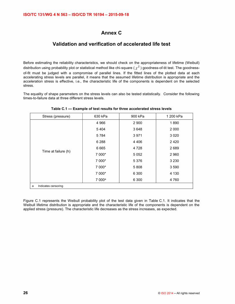
The equality of shape parameters on the stress levels can also be tested statistically. Consider the following times-to-failure data at three different stress levels.

Table C.1 Example of test results for three accelerated stress levels

Stress (pressure) 630 kPa 900 kPa 1 200 kPa

Time at failure (h)

4 966

5 404

5 784

6 288

6 665

7 000*

7 000*

7 000*

7 000*

7 000a

2 900

3 648

3 971

4 406

4 728

5 052

5 376

5 808

6 300

6 300

1 890

2 000

3 020

2 420

2 689

2 960

3 230

3 590

4 130

4 760

a Indicates censoring

Figure C.1 represents the Weibull probability plot of the test data given in Table C.1. It indicates that the Weibull lifetime distribution is appropriate and the characteristic life of the components is dependent on the applied stress (pressure). The characteristic life decreases as the stress increases, as expected.



Figure C.1 Probability plot for an example



Annex D

Calculation procedures for censored data

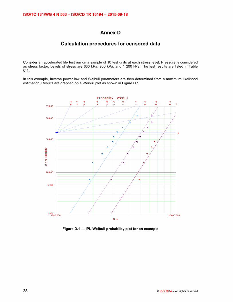
Consider an accelerated life test run on a sample of 10 test units at each stress level. Pressure is considered as stress factor. Levels of stress are 630 kPa, 900 kPa, and 1 200 kPa. The test results are listed in Table C.1.

In this example, Inverse power law and Weibull parameters are then determined from a maximum likelihood estimation. Results are graphed on a Weibull plot as shown in Figure D.1.

Probability - W eibull

Beta=4.5051; K=4.1452E-8; n=1.2453

Time

1000.000 10000.0001.000

5.000

10.000

50.000

90.000

99.000

Figure D.1 IPL-Weibull probability plot for an example



From the Figure D.1, it is possible to approximately estimate the values of scale parameter at three stress levels and common shape parameter.

Life vs Stress

Pressure

100.000 10000.0001000.000500.000

50000.000

1000.000

Figure D.2 Life vs. stress plot for an example

The characteristic life time ( ) corresponding to the stress (pressure) level can be obtained using Figure D.2.

Results determined by software for the Inverse power law (IPL)-Weibull model are;

K = 4,1452E-8

n = 1,2453

=4,5

The IPL-Weibull model can be obtained by putting K, n, and stress level in equation (B.11). If the stress in the normal use condition is 630 kPa, the scale parameter is estimated at;



Acceleration factor (AF) of this example can be obtained by putting accelerated stress level (VA), normal use stress level (VU), and n in equation (B.13).

MTTF under normal use condition is;

Confidence intervals of MTTF with confidence level of 0,95 are (6 019, 8 592) h.

B10 life under normal use condition is;

B10 life: 4 782 h

Confidence intervals of B10 with confidence level of 0.95 are (3 847, 5 943) h.



Annex E

Examples of using accelerated life testing in industrial applications

E.1 Pneumatic cylinder

Pneumatic cylinders are widely used as key components in various industries, like automation production lines. If a failure occurs, there is significant effect on the whole system. Depending on the type of cylinder, a normal use condition life test could take about 30 x 106 cycles (8 400 h). This could be reduced to 2,5 x 106 cycles (700 h) through the use of accelerated life testing.

Leakage caused by seal wear is the main failure mode in a pneumatic cylinder; and temperature and pressure are accelerated stress factors that can be applied to a pneumatic cylinder. It is possible to use a Temperature-Nonthermal model for accelerated life testing of a pneumatic cylinder. The accelerated model and the acceleration factor (AF) of a pneumatic cylinder are determined as follows;

V

Bn eU

CUVL );( (E.1)

AU VVBn

U

A

11

(E.2)

U and V represent the pressure stress and temperature stress (in absolute units). Coefficients C, n and B are calculated from the test data. Subscripts A and U refer to the acceleration condition and normal use condition.

Table E.1 Example of a test plan for pneumatic cylinder

Temperature

S3 (80 ) S2 (90 ) S1 (100 )

Pressure

S3 (140 kPa)

S2 (160 kPa)

S1 (180 kPa)

Table E.1 represents the accelerated life testing plan for pneumatic cylinders. Temperature and pressure level

values (140 kPa, 160 kPa, 180 kPa; 80 , 90 , 100 ) are randomly selected values. Accelerated

coefficients C, n and B should be calculated using test results in the conditions of ~ . The acceleration

factor is calculated from n, B, and stress factors level values in normal use condition, plus the accelerated condition. Life at normal use condition should be estimated using the acceleration factor. Commercial software may be helpful for all of these analyses.



E.2 Flexible hose

Flexible hoses are piping components that conduct fluid (liquid or gas) under pressure. They are significantly important in reliability.

Stressing in accelerated tests for a flexible hose includes pressure, temperature, and half-omega flexing. Table E.2 represents an accelerated life testing plan for flexible hose. One Impulse cycle lasts 1 s. The test is conducted until failure or until the test item reaches a specific number of cycles. Typical failure modes are leakage and fracture.

Table E.2 Example of a test plan for flexible hose

Procedure 1 2 3 4 5 6

Test standard ISO 8032 SAE J517

and SAE J343 ISO 1436,

Type 2A,2B ISO 1436, Type 1A

Maximum working pressure condition

Field condition

Test pressure 150 %

(52,5 MPa)

133 %

(46,5 MPa)

133 %

(46,5 MPa)

125 %

(43,7 MPa)

100 %

(35 MPa)

65 %

(22 MPa)

Temperature (100±3) (100±3) (93±3) (93±3) (55±3) (55±3)

Test pressure waveform

Square Square Square Square Square Square

Half-omega flexing

O O × × O O

Durability (cycles)

- 2,0 105 2,0 105 1,5 105 Until burst Until burst

Figure E.1 Test pressure waveform for flexible hose



Annex F

Palmgren-

The accumulation of fatigue due to multiple stress levels or a spectrum of loads may be covered by Mrule, or the Palmgren-the loads. Eventually, these loads may lead to failure of the component.

Stress-life relationship in accelerated life testing can be explained as follows (see Figure F.1);

(F.1)

where

L is the life of a component

P:is the stress (load)

is the load factor

Figure F.1 Stress-life relationship

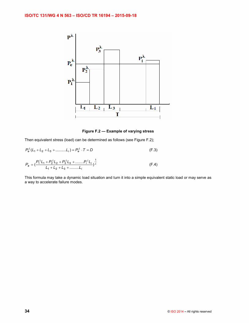
In the case where stress is varying for time T, the stress-life relationship can be written as follows (see Figure F.2);

(Palmgren- (F.2)

where

Li is the operating time for the stress condition i

Pi is the stress for the stress condition i

D is the total accumulated damage



Figure F.2 Example of varying stress

Then equivalent stress (load) can be determined as follows (see Figure F.2);

(F.3)

(F.4)

This formula may take a dynamic load situation and turn it into a simple equivalent static load or may serve as a way to accelerate failure modes.



Annex G

ALT experimental results for pneumatic cylinder

The following slides and their description was a presentation at the ISO pneumatic working group meeting on 2010 October 22.

G.1 Introduction

This is a report on an experimental program for accelerated testing conducted in the laboratory of the Reliability and Assessment Center (RAC) of the Korean Institute of Machinery and Materials (KIMM). The program used over 300 air cylinders from two manufacturers, but tested them in small batches. This is only a status report because the program was still in progress at the time of the presentation.

This report is composed of parts as follows:

1. Introduction: the benefits from accelerated testing and a description of the program;

2. Initial testing to measure the baseline reliability and operational limits;

3. A sampling of the accelerated test results (not all data is shown);

4. Conclusions to-date;

Consider an automated machine and the consequences of downtime. Planned maintenance programs can be developed and carried out at convenient times if the life probability of its components were known (such as B10 life). But, there are many variations to the duty cycle: loads, orientation, and sizes of the

long time. Accelerated testing can reduce the test time and provide the reliability information needed. There are equations for projecting test results from accelerated levels to normal levels. But, confidence in the accuracy of this method requires knowledge and experience. This report describes some of the experience being gained from air cylinder testing.

Preliminary testing was dobaseline reference data. When results are later obtained from accelerated testing, they will be compared to the baseline data to determine accuracy. In addition, a series of high stress tests were made to find the destructive and yield limits similar in concept to the points on a stress-strain curve. This helps determine an operating limit (above the catalog rating) for conducting the accelerated testing.

All phases of this program were conducted in accordance with ISO 19973-Part 3 for cylinders. The high stress tests for determining operating limits used the step stress method as shown in Fig. G.1. Stress was applied to a small number of units in progressively increasing steps until failure occurred.

Figure G.1 Step stress method



G.2 Baseline testing at normal conditions

Figure G.2 shows the rack of test cylinders operating in the KIMM lab, and the mounting arrangement for each cylinder. These were operated at normal condpressure. Samples of cylinders from two manufacturers were independently purchased. The sample size for the normal condition test for Manufacturer A was 9 cylinders; and 8 cylinders for manufacturer B. This phase of the program required a year of testing to fail enough cylinders to obtain sufficient data for analysis.

Fig. G.2 Test rack of cylinders in KIMM lab

Figure G.3 is a bar graph of time to fail each specimen from company A. The test was terminated after 7 of the 9 specimens failed. The cause of failures and test times are shown for each specimen. The failure lives were all obtained from the first failure observed when a specimen exceeded the threshold, as defined in ISO 19973-3. Examination of the cylinders after testing indicated that wear of the piston seals and wear of the cushion seals were the modes of failure.

Fig. G.3 Baseline data at normal conditions for company A



Figure G.4 is a Weibull plot of the failure distribution at normal conditions for company A. The failures are shown as a range the left side is where the last inspection indicated satisfactory operation, and the right side is where the failure was observed. The software draws these symbols and marks (with a dot) the most probable point of failure. The blue line is the median for the best fit of the data to the Weibull equation, and the red curve is the lower 95%, one sided confidence limit. From this, the B10 life at the 95% limit is shown as 3.9162 x 106 cycles.

Fig. G.4 Weibull plot of baseline data for company A

Figure G.5 is a bar graph of time to fail for company B. All eight specimens in this sample failed, but had a mixture of failure causes (all as defined in ISO 19973-3). Examination of failures after testing indicated that wear of piston seals, and blockage of the cushion needle valve hole from debris, were the modes of failure.



Fig. G.5 - Baseline data at normal conditions for company B

Figure G.6 is the Weibull plot of the failure distribution for company B. The B10 life at the 95% lower confidence level is 6.5733 x 106 cycles.

Fig. G.6 Weibull plot of baseline data for company B



G.3 Step stress tests

In the step stress test, two cylinders were used in each of a series of trials. In the first trial, temperature was

operated for 2,000 cycles and stopped for performance measurements. Then the pressure was raised to 15 bar and operated for another 2,000 cycles. After another set of performance measurements, the pressure was raised to 18 bar and operated for another 2,000 cycles. This series of steps were continued until the failure criterion was reached.

Table G.1 shows results of the stress step test for company A using pressure as the steps while temperature wa columns for failure criteria include data for each of the two cylinder units in the test. At 34 bar, the minimum operating pressure was less than the threshold level, which is 1.2 bar. Thus, the failure was determined to occur at 34 bar operating pressure.

Table G.1 2000 cycle pressure step stress data for company A

The same test was repeated with another two cylinders, but using steps of 10,000 cycles (Table G.2). This demonstrates that failure is sensitive to the length of time at a stress level the longer the interval, the lower is the destructive stress. For the 10,000 cycle step test, the minimum operating pressure was less than the 1.2 bar threshold level, at 25 bar operating pressure. Thus, it was determined that the failure occurred at 25 bar.

Table G.2 10 000 cycle pressure step stress data for company A



In both of these tests, the mode of failure was extrusion of the cushion seal not wear as had been observed in the tests at normal conditions (see Fig. G.7). It can be concluded that this is a different mode of failure, even though the performance characteristics measured for threshold comparison were the basis for determining the destructive stress level. Because of this difference the maximum stress levels for accelerated testing must be lowered until failure modes are the same as in the normal condition tests. Thus, the pressure operating limit was chosen below 20, at 16 bar. The chosen pressure operating limit of 16 bar is 133% of the specification limit.

Fig. G.7 Cushion seal failure mode

Another two specimens from company A were then used to conduct step stress tests for temperature. Pressure was held constant at 6.3 bar for this series of tests, and temperature increased as shown in the

mode in this case was piston seal wear same as observed at normal conditions.

The failure occurred at 140 where the minimum operating pressure and the total leakage fell below the threshold level.

Table G.3 2000 cycle temperature step stress data for company A



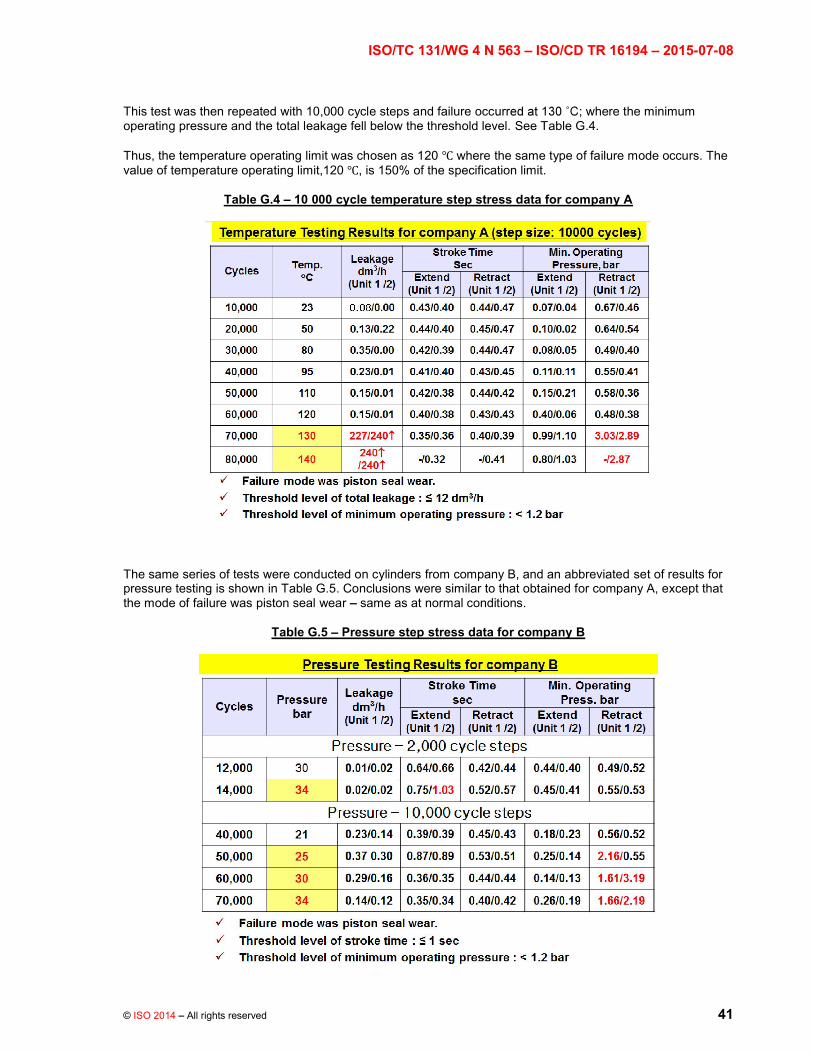
This test was then repeated with 10,000 cycle steps and failure occ ; where the minimum operating pressure and the total leakage fell below the threshold level. See Table G.4.

Thus, the temperature operating limit was chosen as 120 where the same type of failure mode occurs. The value of temperature operating limit,120 , is 150% of the specification limit.

Table G.4 10 000 cycle temperature step stress data for company A

The same series of tests were conducted on cylinders from company B, and an abbreviated set of results for pressure testing is shown in Table G.5. Conclusions were similar to that obtained for company A, except that the mode of failure was piston seal wear same as at normal conditions.

Table G.5 Pressure step stress data for company B



Table G.6 is an abbreviated set of results for temperature step stress testing for company B. For each of the 2,000 and 10,000 cycle step tests, the failure occurred at 150 and 130 respectively; where the total leakage and the stroke time fell below the threshold level.

Table G.6 Temperature step stress data for company B

G.4 Accelerated testing

With data from the destructive step stress tests, a test plan for accelerated testing for company A can be developed as shown in table G.7. Pressure and temperature stress levels are selected to be at levels elevated above the normal conditions - and will also exceed the catalog ratings. However, they are below the destructive levels discovered from the step stress tests.

At this time, tests at the stress levels shown in black number of units have been completed, and tests in red are in progress. Currently, KIMM is putting together test plans for the stress levels that are marked in blue as TBT.

All of these are at single variable stress conditions holding pressure or temperature at one level while testing variations at the other levels. Dual stress conditions are also planned as shown.



Table G.7 Overall test plan for company A

Likewise, a test plan for company B is developed as shown in Table G.8. Again, tests at the stress levels shown in black number of units have been completed.

Table G.8 Overall test plan for company B

The principles of accelerated testing are shown in the two graphs of Figure G.8 one for pressure stress and one for temperature. The blue distribution curves describe a theoretical failure distribution at normal conditions of pressure and temperature. Testing would be conducted at stress levels higher than normal conditions, and their life distributions would be as shown in the three yellow curves labeled first, second and third stress levels. A characteristic of each distribution (mean, B10, or characteristic life), would be projected up to the normal stress level by extrapolation using the equation shown below each graph. This extrapolation provides the equivalent life at normal conditions.



Accuracy of the process is obtained from comparison to real experimental results conducted at normal conditions. With experience, and knowledge of the components, testing at normal conditions could eventually be eliminated. Then, the benefits of reduced test time for reliability by accelerated testing are realized.

Fig. G.8 Accelerated life test concept

Some of the test results at higher stress levels will be shown to demonstrate the process of accelerated testing. The bar graph in Figure G.9 pneumatic cylinders. In this test, some of the specimens were continued on test after observing their first failures as shown on the black bars. However, at this time, only the first failure results are used in the analysis.

Similar data was obtained from testing at 8 bar pressure with longer lives, as expected.

Fig. G.9 Accelerated pressure test data for company A



Partial results are now shown in a composite Weibull graph of Figure G.10. Distributions from the 8 and 12 bar tests are shown plotted, and their characteristic life points, B10 life points, and B10 life at the lower 95% one sided confidence interval are joined by curves. These curves are described by the inverse power law and their projection provides the extrapolation for values at the normal condition. The projected B10 life at the 95% lower confidence level is 4.5702 x 106 cycles. This figure may change after the final distribution from accelerated testing at 14 bar is included.

10 life at the 95% lower confidence level is 3.9162 x 106 cycles indicating that with only partial test results available at this time, the accuracy of the projection is 85.7%.

Fig. G.10 Comparison of results for company A using pressure stress and inverse power law model

The bar graph in Figure G.11 describes results from one of the accelerated temperature tests. Note that the test time was quite short.



Fig. G.11 Accelerated temperature test data for company A

The Weibull graph in Figure G.12 describes the same type of results as the previous one, except that it uses temperature stress which is governed by the Arrhenius equation for extrapolation. This also has only two sets of tests completed at this time, and its projection to the normal conditions is shown in the green distribution. However, these results do not compare favorably to the results from direct testing at normal conditions, as shown in the solid purple distribution.

It is observed that the 95% lower confidence curve is quite bent and this requires further examination. This is an example of the need for experience in selecting the stress levels and understanding the conduct of testing.

Fig. G.12 Comparison of results for company A using temperature stress and Arhenius model



G.5 Conclusions

It was pointed out that accelerated testing reduces the test time, so the amount of time required from the several tests conducted this far is shown in Table G.9. Testing at normal conditions required about one year, and testing at increased pressure levels reduced this by about 100 days, or more. Testing at elevated temperatures resulted in the most significant reduction in test time, but (at this time) has an issue with accuracy that needs more development.

Table G.9 Comparison of test time reduction

The test program at KIMM has initiated research for the fluid power industry in accelerated reliability testing. The program uses components from two manufacturers to expand the variability in this early stage of exploration. Baseline testing for determining accuracy of the accelerated test projections is necessary in this early stage, and has been used for the initial comparisons the pressure type is encouraging; the temperature one is not. Destructive testing has been educational, but does not have to be continued. It is likely that testing to 133% of catalog ratings for the highest stress levels would be a good guideline. It is imperative that failures at the high stress levels be examined to determine if they are the same mode as at normal conditions. If not, the data is not qualified for analysis but may be used for information. The temperature stress method appears to have the most advantage for time savings, but also appears to be the least accurate at this early stage. However, there is much yet to try for a better evaluation.

It is important that accuracy be established in the accelerated test method. This will require some normal condition testing for comparisons before confidence is developed and experience gained. Eventually, the baseline normal condition testing can be phased out and the advantages of reduced test time from accelerated testing can be realized.

A new area for exploration will be combining pressure and temperature stress, to see what advantages and complexities will occur. The temperature acceleration also needs to be evaluated to determine what practices would improve accuracy.

Other laboratories need to begin test programs of their own so that they can begin to acquire experience.



Bibliography

[1] ISO 19973-1, Pneumatic fluid power Assessment of component reliability by testing Part 1: General procedures

[2] ISO 13849-1, Safety of machinery Safety-related parts of control systems Part 1: General principles for design

[3] Elsayed A. Elsayed, Reliability Engineering, Addison Wesley, 1996

[4] James A. McLinn, Practical Accelerated Life Testing, ASQ, 2000

[5] ReliaSoft, Accelerated Life Testing Reference, ReliaSoft Publishing, 2007

[6] Wayne Nelson, Accelerated Testing, Wiley, 2004

[7] William Q. Meeker and Luis A. Escobar, Statistical Methods for Reliability Data, Wiley, 1998

Documents

ISO/TC 131/WG 4 N 566 ISO/CD TR 16194nfpahub.com/wp-content/uploads/2015/10/16194-dtr-For_US_input.pdf · reproduction of working drafts or committee drafts in any form for use by