ISOSLIDER: A System for Interactive Exploration of Isosurfaces

Joint EUROGRAPHICS - IEEE TCVG Symposium on Visualization (2003)G.-P. Bonneau, S. Hahmann, C. D. Hansen (Editors)

ISOSLIDER: A System for Interactive Exploration ofIsosurfaces

Jatin Chhugani, Sudhir Vishwanath, Jonathan Cohen and Subodh Kumar

Department of Computer Science, Johns Hopkins University, Baltimore, Maryland, USA

AbstractWe present ISOSLIDER, a system for interactive exploration of isosurfaces of a scalar field. Our algorithm focuseson fast update of isosurfaces for interactive display as a user makes small changes to the isovalue of the desiredsurface. We exploit the coherence of this update. Larger changes are supported as well. The update to the isosur-face is made at a correct level of detail so that not too many operations need be performed nor too many trianglesneed be rendered. ISOSLIDER does not need to retain the entire volume in the main memory and stores most dataout of core. The central idea of the ISOSLIDER algorithm is to determine salient isovalues where surface topologychanges and pre-encode these changes so as to facilitate fast updates to the triangulation.

Keywords: Volume visualization, Isosurface extraction

1. Introduction

Spatial distribution of scalar data like ‘bone density’, ‘windspeed’ and ‘fluid pressure’ often needs to be visualized inmedical and scientific applications (Figure 8(a)). Many suchapplications involve knowledge discovery, in which scien-tists explore a large field looking for “interesting” charac-teristics. Two common ways of visualizing these fields aredirect volume rendering 4 and isosurface computation 12, 15.Direct volume rendering produces a color at each pixel thatis the composition of the scalar values at points intersectedby a ray through that pixel. Isosurface visualization requirescomputation and display of all points (i.e., surfaces in athree-dimensional field) in the data with a given scalar value.

One common modus operandi for data exploration is tocontinuously vary the desired isovalue, generate the result-ing isosurface and see how the surface changes as it slidesfrom value to value. Our algorithm addresses the need forsuch isosurface exploration and is designed to take full ad-vantage of the resulting coherence. In addition, our algo-rithm works well with large data sizes by allowing most ofthe data to reside on the disk at the exploration time. Its fo-cus is on interactive isosurface update so that the scientistmay easily maintain the context as the isovalue changes.

Formally, a volumetric scalar field is represented by theset of tuples <(Si, pi)>, i = 0..N, such that Si is the scalar

value at point pi ∈ <3. The points pi are usually selected tolie on a grid (structured or unstructured). Adjacent points onthe grid are connected to form a cell. We sometimes denoteSi as S(pi) to be explicit. Furthermore, S(p) at points pnot in the tuple set are computed from cell’s Sis (usually bytri-linear interpolation). Isosurface of a field, ψλ, at scalarvalue λ is the set of all points p, such that S(p) = λ. Variantsof the Marching Cubes algorithm 15 are commonly used tocompute ψλ.

The Marching Cubes algorithm finds the overall surfaceby processing every cell in the input. The computation percell is O(1). Recent isosurface algorithms reduce the num-ber of cells considered by predicting the active cells: thecells, which actually contain the desired isovalue. The searchfor active cells takes one of three forms: spatial search 10,range search 3 or surface growth 1. Spatial search techniquessubdivide space and hierarchically eliminate partitions thatdo not contain an active cell. Range search methods asso-ciate each cell with the range of values it contains. Thesethen search for the ranges that contain the desired isovalue.Surface growing methods start with some active cell(s) andfind other active cells by tracking surface adjacencies. Rangebased methods are the most general and can handle unstruc-tured cells, even if they do not directly benefit from spatialcoherence of computations. Our algorithm is range based,

c© The Eurographics Association 2003.

Chhugani et al / ISOSLIDER

appropriately modified to exploit spatial coherence. Whilethe framework of our algorithm can trade off time and diskrequirements, in our current implementation we have cho-sen to favor fast computation over disk requirement. Also,we currently handle uniform (voxel) grid input only. Whileone may handle curvilinear and unstructured grids by con-verting them to a uniform grid 11 first, our algorithm can beeasily extended to directly handle such data.

The main idea of our algorithm is to realize that smallchanges in isovalues require small changes to active cells.By simply pre-computing these changes and storing themout-of-core we can find the active cells quickly. Note thatthe isovalues at which a topological change happens are allin Si (In case of trilinear interpolation, topology changes canoccur inside a cell as well, but are directly handled by therender-time algorithm). Hence, in principle, we merely needto store <Si, pi> sorted by their values Si. Every time weslide past an isovalue, Si, the cells adjacent to pi are inacti-vated or activated or sometimes simply re-triangulated. Weaugment this simple scheme to allow efficient sliding of iso-surfaces across small as well as large values. In addition, weincorporate multi-resolution isosurface construction into ourscheme. Our in-memory data structure also allows re-use ofmost topological information from frame to frame. Only in-terpolations of values need be computed afresh.

1.1. Previous Work

Span-space computation of Livnat et al.14 achieved O(√

N)search time for active cells. The interval-tree based searchof Cignoni et al.3 reduced that further to O(logN), whichwas extended for out-of-core searches by Chiang et al.2. In-terval tree has an optimal worst case complexity for rangesearch but is not well suited for sequential out-of-core ac-cess of successive intervals. While it is possible to augmentthe interval tree with ‘next-in-sequence’ links, we have optedfor a simpler data structure based on skip-lists 17 that workswell for isosurface sliding. The idea of using such local up-dates has been applied before. Giles and Haimes7 maintainedtwo lists: minlist, sorted by the minimum values of each celland maxlist, sorted by the maximum value of each cell. Ifthe isovalue is changed by a small value from λ0 to λ1, allintervals beginning in the range [λ0-λ1] are added as po-tential active cells. The list is then purged of inactive cells.The performance for large changes in λ is O(N). Shen andJohnson19 improve the average performance by transformingthe maxlist into sweeping list by adding a flag for each entrymarking whether the minimum value of the correspondingcell is less than the current isovalue. The worst case perfor-mance remains O(N + K), K being the size of the resultingtriangulation 19. Our algorithm performs work independentof N and is proportional only to δK, the change in triangu-lation at each frame for small changes in isovalue. For largechanges in the isovalue, the total work is still O(logN + K)

on average. The main advantage of our work is its out-of-core operation.

One problem with the Marching Cubes algorithm is thatit generates a large number of polygons, up to five per cell.For large volumes, especially voxel grids, this is usually toomany. Ramachandran et al.20 present a non-interactive view-dependent algorithm for isosurface extraction on a cluster ofmachines. Dynamic simplification 9, 5 of isosurfaces is tooslow to be interactive, however, and direct cell simplifica-tion schemes are popular 10, 18. Most focus on using hierar-chically larger cells composed of input cells when the re-sulting interpolation error is small. Some allow controlledsimplification of topology 6. Most are able to produce dras-tic simplification at high error allowance. Gregorski et al.8,in particular, reports near interactive performance by enforc-ing a limit on the number of operations performed per frame.Their algorithm is designed for view-dependent updates to agiven isosurface. Isosurface updates are slower, unless theerror threshold is turned very high. Our algorithm performsconservative and static simplification only. The resulting tri-angles can be further simplified in a view-dependent fashion,but that is not currently done in our system.

2. ISOSLIDER algorithm

The main steps of isosurface visualization are as follows:

1. Find the active cells2. Find the active edges for each cell3. Classify each cell and compute the adjacencies of result-

ing triangles4. Find the vertices on the active edges (location and nor-

mal)5. Send the resulting triangles to the graphics card

A note about Step 5: it must be performed every framethat the isovalue changes. As the resulting isosurface slides,the vertex positions change. One might consider performinginterpolations on the graphics card. However, many appli-cations require the surface to be on the CPU for geometricanalysis. We have chosen to perform the interpolations onthe CPU. Note that for small changes in λ, most cells remaineither active or inactive during the slide. Furthermore, thesame edges of the active cells usually remain active imply-ing that the cell maintains the same classification and usesthe same triangle adjacencies. We exploit coherence at allthese levels.

To find the active cells (Step 1), we preprocess the data.Consider a cell, C, with points pC

j , j = 1..k, sorted by theirscalar values, i.e., SC

j < SCj+1. Recall that C is active only

for isovalues SC1 ≤ λ ≤ SC

k . Thus, as we slide the isosur-face from λ1 to λ2, cell C becomes active or inactive whenwe cross SC

1 or SCk . We could then recompute the triangula-

tion for those cells that change their status. Note also thatthe topology of triangles generated by C changes only at



λ = SCj , j = 1..k. If we maintain a sorted list of all scalar val-

ues in the field, S j, j = 1..N, we know that the topology ofsome cell changes each time λ crosses an S j . If we store thisinformation, we obtain an algorithm that does not need totouch any cell that does not undergo a change in its triangu-lation. We nominally store the following information blockB j with each S j in our sorted list:

1. p j2. E+: the list of indices of the edges that become active3. E−: the list of indices of the edges that become inactive4. S+: the list of scalar values S(pl) for each point pl such

that edge p j pl ∈ E+

5. S−: the list of scalar values for edges in E−

For high quality shading, we also retain the normals at p jand all pl . This naive approach replicates each input pointfor each adjacent edge. This can be avoided at the cost ofadditional disk I/O by using a point layout similar to thatused by Gregorski et al.8.

Note that the main drawback of this approach is that largechange in λ requires several blocks to be read from the diskresulting in slow isosurface update even if the blocks arestored contiguously on the disk. We solve this problem byusing a skip list of blocks.

2.1. Skip-list

Block B j provides all changes to the active list when theisovalue changes from a value λ1 ∈ [S j−1,S j] to λ2 ∈[S j,S j+1]. In general, if the isovalue λ1 ∈ [Sm−1,Sm] goesto λ2 ∈ [Sn,Sn+1], all blocks Bm..Bn are required. Unfortu-nately, this larger isovalue change could require O(N) workin reading and applying the blocks. If the maximum numberof active edges involved is K = E(λ1) + E(λ2), we wouldlike to limit the work performed to more like O(K). Us-ing a skip-list approach 17, we can reduce the actual workto O(logN +K).

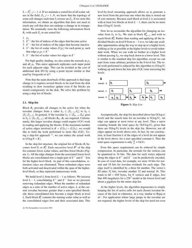
In the skip-list structure, the original list of blocks Bi be-comes level 0, or B0

i . Each successive level BL of the skiplist contains fewer scalar values, and thus fewer blocks (Fig-ure 1). All the edge changes from the associated lower-levelblocks are consolidated into a single pair of E+ and E− listsfor the higher-level block. As part of this consolidation, re-dundant edges are eliminated. These redundant edges wereboth activated and deactivated within the span of the higher-level block, so they represent unnecessary work.

We build level L from level L−1 as follows. We traverselevel L− 1, consolidating E+ and E− lists as we proceed,removing redundant edges. When the number of redundantedges as a ratio of the number of active edges, k, at the cur-rent isovalue becomes greater than a user-specified thresh-old, these consolidated lists become a single block at levelL. Each block BL

i contains the starting scalar value as well asthe consolidated edges lists and their associated data. This

level-by-level streaming approach allows us to generate anew level from the previous one when the data is stored outof core memory. Because each block at level L is associatedwith at least two blocks at level L−1, there can be no morethan O(logN) levels.

Now let us reconsider the algorithm for changing an iso-value from λ1 to λ2. We start at block B0

m−1 and wish toreach block B0

n. Rather than reading and applying all the in-dividual blocks on level 0 from m−1 to n, we take any avail-able opportunities along the way to step up to a higher level,walking as far as possible at the higher levels to avoid redun-dant work. When we can walk no further at a higher levelwithout passing λ2, we step back down to a lower level. Thisis similar to the standard skip list algorithm, except we canstart from some arbitrary position in the 0-level list. The to-tal work performed is reduced by this algorithm to O(logN)walking up and down the lists plus O(K) time traversing thelevels.

S1

SaS1

Sb SdScSaS2

Sd

S1 Sd

Level 0

Level 2

Level 1

Figure 1: Skip List

Asymptotically, the skip list described above has O(logn)levels and the search time for an isovalue is O(logN). Anedge can appear at most twice at any level. Thus a naivecounting bounds the total space by O(N logN), given thatthere are O(logN) levels in the skip list. However, not alledges appear on levels above zero. In fact, by our construc-tion, at least fraction k of the edges of a level do not appearin the level above, for a user specified constant k. Thus thetotal space requirement is only N

k = O(N).

Even this space requirement can be reduced by simplecompression. In particular, the normals for the vertices canbe quantized to 16 bits. The data for each vertex adjacentalong the edges in E+ and E− can be predictively encoded.In case of voxel data, for example, we store 10 bits for nor-mal and 10 bits for isovalue residuals for each edge. Theedge itself is identified by a three bit number. The vertex’sID takes 32 bits, isovalue another 32 and normal 16. Thistotals to 6E + 10N bytes, for N vertices and E edges, lessthat 400 megabytes for a 2563 model at the lowest level andabout a gigabyte for the entire skip list.

At the higher levels, the algorithm degenerates to simplykeeping the list of active cells for each chosen isovalue be-cause of the lack in coherence, in a way similar to Bajaj etal.1. For application where large jumps in the isovalue arenot required, the higher levels of the skip list need not even



be precomputed and computed online when necessary. Weusually only precompute 4-5 levels and leave the rest un-generated, which may be computed in a lazy fashion.

2.2. Level of Detail

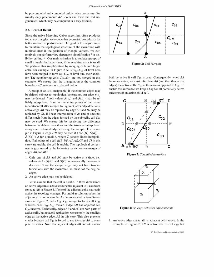
Since the naive Marching Cubes algorithm often producestoo many triangles, we reduce this geometric complexity forbetter interactive performance. Our goal in this algorithm isto maintain the topological structure of the isosurface withminimal error in the position of triangle vertices. We cur-rently do not perform view-dependent simplification 8 or vis-ibility culling 13. Our main criterion is to replace groups ofsmall triangles by larger ones, if the resulting error is small.We perform this simplification by merging cells into largercells. For example, in Figure 2 cells C00..C03 of level zerohave been merged to form cell C10 of level one, their ances-tor. The neighboring cells C04..C07 are not merged in thisexample. We ensure that the triangulation at the commonboundary AC matches as explained below.

A group of cells is ‘mergeable’ if the common edges maybe deleted subject to topological constraints. An edge pi p jmay be deleted if both values S(pi) and S(p j) may be re-liably interpolated from the remaining points of the parent(ancestor) cell after merger. In Figure 3, after edge deletions,active edge AB may be replaced by edge AC and HI may bereplaced by GI. If linear interpolation of ac and gi does notdiffer much from the edges formed by the sub cells, cell C10may be used. We ensure this by restricting the differencebetween the deleted isovalues and the isovalue interpolatedalong each retained edge crossing the sample. For exam-ple in Figure 3, edge HB may be used if (I(S(H),S(B))−S(E)) < ∆ for a small ∆, where I denotes linear interpola-tion. If all edges of a cell (HB,DF,AC,AG,GI and CI in thiscase) are usable, the cell is usable. The topological correct-ness is guaranteed by the following restrictions on merger ofedges AB and BC:

1. Only one of AB and BC may be active at a time, i.e.,values S(A),S(B), and S(C) monotonically increase ordecrease. Since the merged edge may not have two in-tersections with the isosurface, so must not the originaledges.

2. An active edge may not be deleted.

Let us assume that the cell is a cube. In three dimensionsan active edge must activate four cells adjacent to it as shownfor edge AB in Figure 4. If one of the adjacent cells is alreadyactive, its topology changes. For multi-resolution cubes theadjacency is not as simple. As demonstrated in two dimen-sions in Figure 2, cells C00..C03 merge to form cell C10,whereas cells C04..C07 remain. Edge AB has adjacent cellC00 inactive. Technically, edges AB and AC are both parts ofactive cells, but to avoid replication we use only the smallestedge as the active edge, AB in this case. This also preventscracks because cell C10 is forced to use the edge AB to com-pute its vertex. Note that adjacent edges AB and BC cannot

A

B

C

C04

C06

C07C10

C05 C01

C03

C02

C00

Figure 2: Cell Merging

both be active if cell C10 is used. Consequently, when ABbecomes active, we must infer from AB (and the other activeedges) the active cells: C10 in this case as opposed to C00. Toenable this inference we keep a flag for all potentially activeancestors of an active child cell.

A B C

D

ab

hi

ac

E

G

FC10

C01

C03

C02

C00

giH I

Figure 3: Simplified isosurface

A B

C1

C4

C2

C3

Figure 4: An edge activates adjacent cells

1. An active edge marks all its adjacent cells active. In theexample in Figure 2, AB is active due to cell C07 but



marks C07 as well as C00. C00 is marked erroneously inthis case.

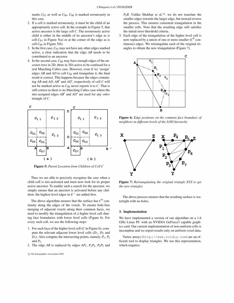
2. If a cell is marked erroneously, it must be the child of anappropriately active cell. In the example in Figure 5, thatactive ancestor is the large cell C. The erroneously activechild is either in the middle of its ancestor’s edge as iscell C03 in Figure 5(a) or at the corner of the edge as iscell C00 in Figure 5(b).

3. In the first case, C03 may not have any other edges markedactive, a clear indication that the edge AB needs to becontributed to an ancestor.

4. In the second case, C00 may have enough edges of the an-cestor (two in 2D, three in 3D) active to be confused for areal Marching Cubes case. However, even if we ‘assign’edges AB and AD to cell C00 and triangulate it, the finalresult is correct. This happens because the edges contain-ing AB and AD, AB′ and AD′, respectively of cell C willnot be marked active as C00 never reports it to C. That isstill correct as there is no Marching Cubes case where themis-assigned edges AB′ and AD′ are used for any othertriangle of C.

(a) (b)

C01

C00 C03

C02

A B

C13

C11 C12

C01

C00 C03

C02 C13

C11 C12

A B

D

CC

C07 C07B'

D'

Figure 5: Parent Location from Children of Cell C

Thus we are able to precisely recognize the case when achild cell is mis-activated and must now look for its properactive ancestor. To enable such a search for the ancestor, wesimply ensure that an ancestor is activated before any chil-dren: the highest level edges in E+ are added first.

The above algorithm ensures that the surface has C0 con-tinuity along the edges of the voxels. To ensure hole-freemerging of adjacent voxels along their common faces, weneed to modify the triangulation of a higher level cell shar-ing face boundaries with lower level cells (Figure 6). Forevery such cell, we use the following steps:

1. For each face of the higher level cell (C in Figure 6), com-pute the relevant adjacent lower level cells (D1, D2 andD3). Also compute the intersecting points, namely, P1, P2and P3.

2. The edge AB is replaced by edges AP1, P1P2, P2P3 and

P3B. Unlike Shekhar et al.18, we do not translate thesmaller edges towards the larger edge, but instead reversethe process. This ensures consistent triangulation in thesmaller cells. Note that the resulting edge still satisfiesthe initial error threshold criteria.

3. Each edge of the triangulation of the higher level cell isnow replaced by a union of one or more smaller (C0 con-tinuous) edges. We retriangulate each of the original tri-angles to obtain the new triangulation (Figure 7).

A

B

D

D

D

P

P

P

1

1

22

33

C

Figure 6: Edge positions on the common face boundary ofneighbors in different levels of the LOD hierarchy

X

Y

Z Z

Y

X

PP

P

P

P

P

P

16

54

3

2

7

Figure 7: Retriangulating the original triangle XYZ to getthe new triangles

The above process ensures that the resulting surface is wa-tertight with no holes.

3. Implementation

We have implemented a version of our algorithm on a 1.6GHz Linux PC with an NVIDIA GeForce3 capable graph-ics card. Our current implementation of non-uniform cells isincomplete and we report results only on uniform voxel data.

Vertex arrays (http://www.nvidia.com) are an ef-ficient tool to display triangles. We use this representation,which requires:



• V : a contiguous list of all vertices used in the triangles and• T : a contiguous list of all triangles, each triangle specified

by three indices into V .

We recompute V every frame the isosurface changes butreuse most of T . In order to reuse the indices of T , it isimportant to update V coherently. We also retain the activeedges and cells in the main memory from frame to frame.We assume the triangle, edge and cell information fit in themain memory. (For very large datasets that do not allow that,it is possible to use the ‘metacell’ scheme of Chiang et al.2

to process a subset of the data at a time.)

3.1. Precomputation

The precomputation step sorts (using external memory sort-ing) the input scalar values and constructs the skip list in abottom-up traversal, level by level. First, it computes the er-ror of each hierarchically constructed cell from its children’svalue. We use an error bound of 1% of the total range of iso-values. Any active edge with larger error is not merged. Thesorted tuples <Si, pi>, are next traversed as follows. At eachstep of level zero, we consider all edges connected to the cor-responding point pi. We find the edges connected to pi thatbecome active and those that become inactive when cross-ing the isovalue from below it to above it. The new edgesare tested in the order of their size. The largest edge usableis added to E+. If an added edge causes a new topologicalconstraint violation in any adjacent cell, that cell is subdi-vided. Deleted edges are added to E−. Each deleted edge isnext tested for topological constraints. If the edge was con-straining an adjacent cell, that cell is retested for merger. Allinformation of the affected edges is collected and appendedto the end of the file. Merge and Split records are stored asthe ID of the edge and the count of how many times it maymerges or splits. For example, if an edge AB merges to itsgrandparent, we store its ID and the count 2.

3.2. In-core data structure

We maintain the following data structures at the renderingtime:

• An Edge information array (E), which maintains the infor-mation related to each active edge. Specifically, we storethe vertex coordinates (V1), isovalue (S1) at the startingpoint of the edge, the normal values at the two end-pointsof the edge (N1 and N2), the gradient in the vertex coordi-nates ∂V = V2−V1

S2−S1. In order to expedite the computation

of the unit normal at run-time, we also maintain a valuem = 2sin2(α/2), where α is the angle between N1 andN2. For the interpolating parameter value t, the norm ofthe normal is given as 1√

1−2mt(1−t), for small 2mt(1− t).

We use the Taylor’s expansion to evaluate the norm, thusavoiding the expensive square-root operation.

• An array of list of indices (I) forming the triangles. These

indices represent the vertex indices which form each tri-angle. The marching cubes algorithm can generate up tofive triangles for each active voxel. We maintain five dif-ferent lists, list i for triangles of voxels with i triangles.The triangles of each cell are stored contiguously in itscorresponding list. As a cell undergoes a change in thenumber of its triangles, this contiguous set is deleted fromthe old list and transferred to another if needed. This buck-eting by triangle set cardinality allows effective memorymanagement. All triangle sets in list i are the same sizeand a hole created by a deleted set can be easily filled byanother set.

• An array of vertex Values (V). Each entry in this arraycorresponds to the interpolated vertex value from the Edgearray E.

• An array of unit length Normals (N). Each entry in this ar-ray corresponds to the normal value at the correspondinglocation in the Vertices Array V.

• Hash tables, HE and HC, for the active edges and the ac-tive Cells respectively. HE stores a tuple <gid, id>, wheregid is the identifier (ID) for the edge, and id is its locationin E. gid is formed from the edge’s location, direction,and its level in the Level-of-Detail hierarchy. HC storesfor each voxel, the tuple <vid, Start Address, list_number,case_number>. Here vid is the identifier of the voxelwhich is formed from its position in space and its levelin the LOD hierarchy. list_number refers to the number oftriangles the voxel has at that instant, Start Address refersto its starting index in I, and case_number refers to thecase number of the Marching Cubes table used for thisparticular voxel. We use a hash function from the familyof hash functions H = {ha,b|a,b ∈ Zp}, with a 6= 0. ha,bis defined as ha,b(x) = g ( fa,b(x)), where g : Zp → N ,given by g(x) =x mod n, and fa,b(x) = (ax + b) mod p.Here p is a large prime number (greater than the largestentry being hashed to the table), and n is the size of thehash table. The size of the hash table is chosen to betwice the average number of edges expected to be active(O(N

23 )), where N is the total number of sampled points in

the data set. This family of hash functions is proven to bestrongly 2-universal 16, thereby reducing the probabilityof collisions. We stress that such a hash function is neces-sary for attaining real-time rates with our algorithm (Ex-pected O(1) search time). We maintain open chain hash-ing, i.e. all the entries colliding at one specific location ofthe hash table are linked together in a link-list.

3.3. Sliding

As the user slides the isovalue, two kinds of updates are re-quired: change of the active edge list and computation of theinterpolated vertex and normal coordinates.

Once the active edge list is fixed, only the arrays V and Nneed to be changed. A specific entry Vi is changed by ∇Vi =



∂S * ∂Vi (stored in E). Similarly, the normal is interpolatedfrom N̂1 and N̂2, and scaled by its length to normalize it.

If the active edge list changes, these additions and dele-tions are stored in lists Add and Delete respectively. We pro-cess the Delete list before accessing the Add list to avoidfragmentation in the various arrays. Each entry of the Deletelist contains an edge ID, which is then hashed (using HE) tothe Edge information array (E), and deleted from both lists.The IDs of cells adjacent to the edge is hashed to obtain theirindices in HC. The case mask of each cell is changed. Also,the Start_Address and list_number fields of the cell becomestale. The corresponding entries in I are deleted, fragmentingthese arrays temporarily. Next, the Add list is processed, anda new entry is inserted for this edge into HE and E (therebyfilling up the holes created by the deletions). Again, HC ismodified, and the corresponding case masks are updated. Incase the number of additions is smaller than the number ofdeletions, E and I are compacted. We fill the holes by trans-ferring entries from the end of the list into them. When anedge entry is moved, its cells are re-accessed and their af-fected triangle’s indices are modified to the edge’s new loca-tion.

Once the topology has been changed, the vertex and nor-mal lists are regenerated from E. Finally, V, N and I are sentto the graphics pipeline.

4. Results

We have tested our algorithm on a variety of models. In Ta-ble 1, we report the several features of the five major mod-els we used. The number of distinct isovalues in a dataset isan indication of how often we have to compute the changein topology (Figure 9) and store the changes. The BostonTeapot is a 8-bit quantized data set, while the BluntFin (Fig-ure 8(b)), CT Head Scan and the Spherical Shell models are16-bit quantized data sets, and hence the distinct isovalue setspans almost the entire range, symbolizing greater changeswhen these values are crossed. The RADMRI dataset has32-bit floating point values at the voxel end points. Thisprovides for a wider range of values for a given resolutionmodel.

The average number of active edges refers to the voxeledges intersected by the isosurface. Our run-time memoryconsumption is proportional to the number of intersectingvoxels (around 40V bytes, where V is the number of inter-secting voxels), and not the whole model. This coupled withthe level-of-detail aids in rendering high resolution modelsat near real-time frame rates.

In Table 2, we give timings and the storage requirementsfor the preprocessing algorithm. During pre-processing, westore the edge ids for all the changes. In Table 3, we show thetime taken when the user makes a big change in the isovalueto be rendered. For very small changes, we can change theisosurface in less than a millisecond, without affecting the

Model Resolution Distinct Avg. No. of

isovalues Active Edges

RADMRI 69x261x69 904,216 176,104

BluntFin 256x256x256 54,268 402,918

Spherical Shell 256x256x256 33,743 176,504

Boston Teapot 256x256x256 236 320,382

CT Head Scan 512x512x252 259 803,113

Table 1: Details of the models used for experimentation

Model Error Pre-proc. Change in Disk

(%) Time active edges Space

RADMRI 0.1 2.9 min. 27,435 21 MB

BluntFin 0.2 5.1 min. 72,196 320 MB

Sph. Shell 0.2 4.5 min. 65,234 300 MB

Bos. Teapot 0.7 16.4 min. 85,556 281 MB

Head Scan 0.8 44.6 min. 203,139 800 MB

Table 2: Details of the preprocessing algorithm

frame rates. For appreciable changes, we take around 0.1 -0.27 seconds for changes as large as 1-10% of the total rangeof isovalues. The average increase in the number of updatesreduces as the step size increases, as some of the redundantchanges cancel each other. For small changes in the isovalue,we obtain rendering rates of 10-20 frames per second, whichdrops to around 5-6 frames a second in case of large changes.For small changes, the frame rate is still mostly dominatedby the triangle rendering performance of our machine (1.6GHz PC with GeForce3 graphics card running Linux). Dur-ing run-time, only a small percentage of time (around 0.04seconds per frame) is spent in interpolating the vertex andnormal values (and normalizing them).

5. Conclusion

We have developed an out-of-core coherent algorithm forfast isosurface extraction. The target application is one inwhich small changes to isovalues are made to try to discoverand study the topological changes near some isovalues. Thealgorithm achieves efficiency by ensuring that most infor-mation unchanged from the previous extraction is not evenaccessed. In our experience this algorithm provides a fasteralternative to ones that recompute the isosurface by startingat the top of a hierarchy (like the interval tree).

Part of this fast performance comes at the cost of replicat-ing each piece of data with all its adjacent data. While disk



Model Change in Average Updates Update

isovalue (%) per frame Time (sec)

RADMRI 0.1 3,500 0.008

RADMRI 1 29,316 0.07

RADMRI 5 88,481 0.21

RADMRI 10 116,296 0.27

BluntFin 1 64,185 0.14

BluntFin 2 80,068 0.2

BluntFin 5 76,877 0.19

BluntFin 10 71,453 0.17

Table 3: Run-time behavior of our algorithm

space is cheap, this still incurs a four to six fold increaseover the original data. We are investigating smooth tradeoffsin replicating only some data and exploiting disk-cache co-herence to fetch neighboring data.

Acknowledgments

The CT scan of the head was provided by the Depart-ment of Computer Science of Johns Hopkins University. TheRADMRI dataset was provided by Julian Krolik of the De-partment of Physics and Astronomy of Johns Hopkins Uni-versity. The Boston Teapot model was downloaded fromhttp://www.volvis.org. We would like to thank the anony-mous reviewers for their useful comments.

References

1. C. L. Bajaj, Valerio Pascucci, and Daniel Schikore. Fastisocontouring for improved interactivity. In Symposiumon Volume Visualization, pages 39–47, 1996.

2. Yi-Jen Chiang, Cláudio T. Silva, and W. J. Schroeder.Interactive out-of-core isosurface extraction. In DavidEbert, Hans Hagen, and Holly Rushmeier, editors,Proc. IEEE Visualization, pages 167–174, 1998.

3. P. Cignoni, P. Marino, C. Montani, E. Puppo, andR. Scopigno. Speeding up isosurface extraction usinginterval trees. IEEE Transactions on Visualization andComputer Graphics, 3(2):158–170, 1997.

4. R. Drebin, L. Carpenter, and P. Hanrahan. Volume ren-dering. Computer Graphics, 22(4):65–74, 1988. Pro-ceedings of SIGGRAPH ’88.

5. M. Garland and P. Heckbert. Surface simplification us-ing quadric error metrics. In Proc. ACM SIGGRAPH,pages 209–216, 1997.

6. T. Gerstner and R. Pajarola. Topology preserving andcontrolled topology simplifying multiresolution isosur-face extraction. In T. Ertl, B. Hamann, and A. Varsh-ney, editors, Proc. IEEE Visualization, pages 259–266,2000.

7. M. Giles and R. Haimes. Advanced interactive visu-alization for cfd. Computing Systems in Engineering,1(10):51–62, 1990.

8. B. Gregorski, M. Duchaineau, P. Lindstrom, and V. Pas-cucci. Interactive view-dependent rendering of largeisosurfaces. In Proc. IEEE Visualization, 2002.

9. H. Hoppe. Progressive meshes. In Proc. ACM SIG-GRAPH, pages 99–108, 1996.

10. J.Wilhelms and A. Van Gelder. Octrees for faster iso-surface generation. ACM Transactions of Graphics,11(3):201–227, 1992.

11. J. Leven, J. Corso, J. D. Cohen, and S. Kumar. Interac-tive visualization of unstructured grids using hierarchi-cal 3d textures. In Proceedings of IEEE Symposium onVolume Visualization and Graphics 2002, 2002.

12. M. Levoy. Display of surfaces from volume data. IEEEComput. Graphics Appl., 8(3):29–37, 1988.

13. Yarden Livnat and Charles Hansen. View dependentisosurface extraction. In David Ebert, Hans Hagen,and Holly Rushmeier, editors, Proc. IEEE Visualiza-tion, pages 175–180, 1998.

14. Yarden Livnat, Han-Wei Shen, and Christopher R.Johnson. A near optimal isosurface extraction algo-rithm using the span space. IEEE Transactions on Vi-sualization and Computer Graphics, 2(1):73–84, 1996.

15. W. Lorensen and H. Cline. Marching cubes: A high-resolution 3d surface construction algorithm. In ACMSIGGRAPH’87, pages 163–169, 1987.

16. R. Motwani and P. Raghavan. Randomized Algorithms.Cambridge University Press, 1995.

17. William Pugh. Skip lists: A probabilistic alternative tobalanced trees. In Workshop on Algorithms and DataStructures, pages 437–449, 1989.

18. R. Shekhar, E. Fayyad, R. Yagel, and F. Cornhill.Octree-based decimation of marching cubes surfaces.In Proc. IEEE Visualization, pages 335–342, 1996.

19. Han-Wei Shen and Christopher R. Johnson. Sweepingsimplices: A fast iso-surface extraction algorithm forunstructured grids. In Proc. IEEE Visualization, pages143–150, 1995.

20. V. Ramachandran X. Zhang, C. Bajaj. Parallel and out-of-core view-dependent isocontour visualization usingrandom data distribution. In Proc. of the Joint Eu-rographics IEEE TVCG Symposium on Visualization,2002.



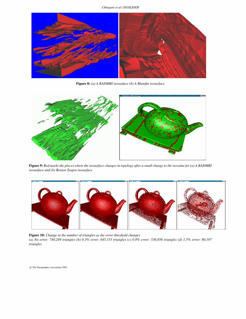
Figure 8: (a) A RADMRI isosurface (b) A Bluntfin isosurface

Figure 9: Red marks the places where the isosurface changes in topology after a small change to the isovalue for (a) A RADMRIisosurface and (b) Boston Teapot isosurface

Figure 10: Change in the number of triangles as the error threshold changes(a) No error: 740,249 triangles (b) 0.3% error: 645,153 triangles (c) 0.8% error: 536,856 triangles (d) 1.5% error: 80,197triangles


Documents

ISOSLIDER: A System for Interactive Exploration of Isosurfaces