Isosbestic Points and Kinks: Fingerprints of Electronic Correlations

Dieter Vollhardt

Supported by Deutsche Forschungsgemeinschaft through SFB 484

Symposium celebrating Prof. Dr. Hilbert v. Löhneysen‘s 60th Birthday;

Karlsruhe, October 27, 2006

LT18, Kyoto; August 1987

Aspen Winter Conference on Condensed Matter PhysicsAspen, January 1991

Aspen Winter Conference on Condensed Matter PhysicsAspen Center for Physics, January 1991

Aspen Center for Physics: Hilbert space

4th Japanese-German SymposiumKii-Katsuura; September 1996

6th Japanese-German SymposiumSapporo, September 2000

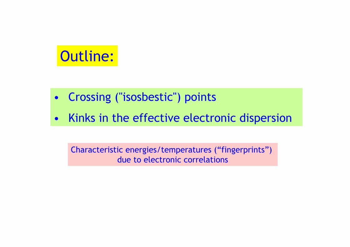
• Crossing ("isosbestic") points

• Kinks in the effective electronic dispersion

Outline:

Characteristic energies/temperatures (“fingerprints”) due to electronic correlations

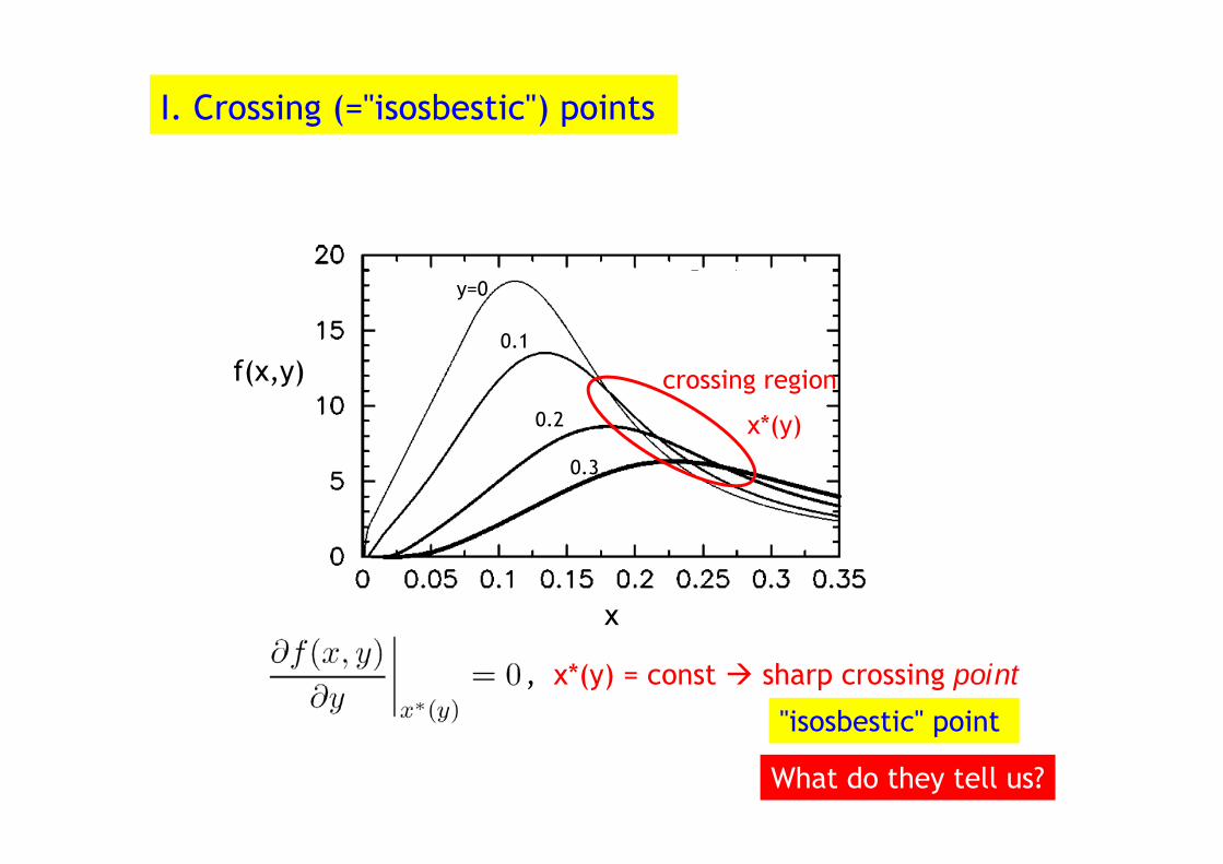
x

f(x,y)

y=0

0.1

0.2

0.3

x*(y)

crossing region

, x*(y) = const sharp crossing point

"isosbestic" point

I. Crossing (="isosbestic") points

What do they tell us?

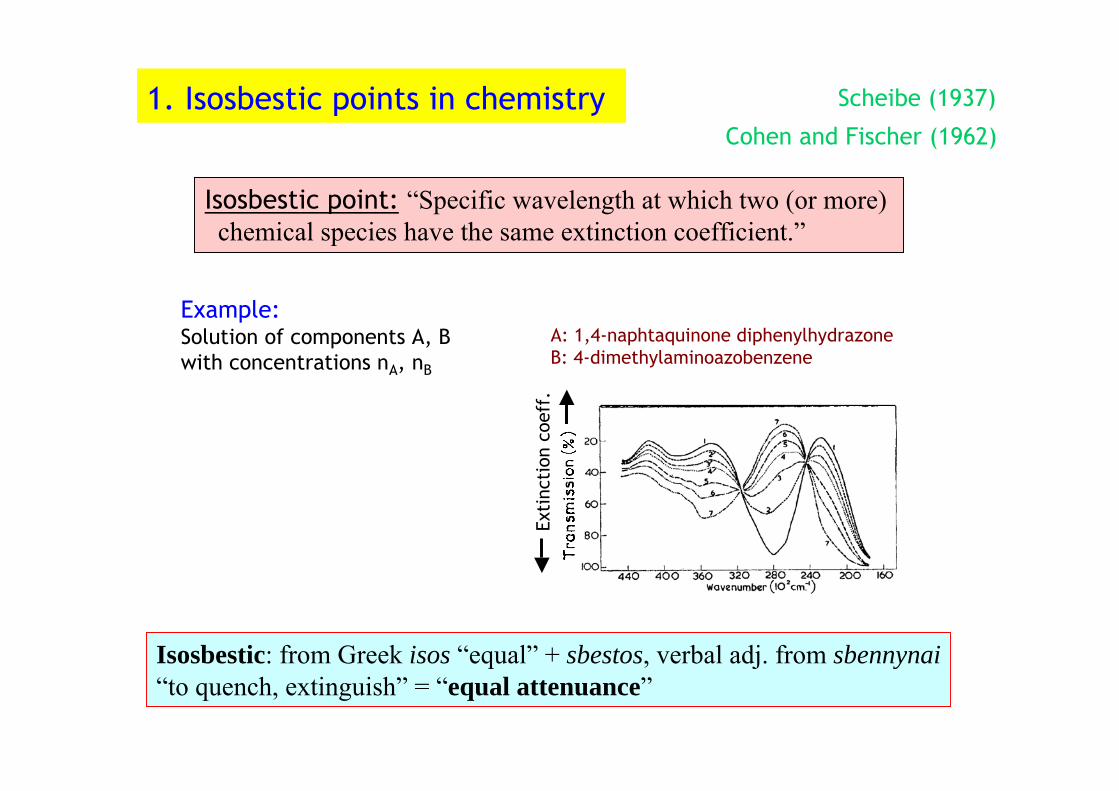
Isosbestic point: “Specific wavelength at which two (or more) chemical species have the same extinction coefficient.”

Scheibe (1937)1. Isosbestic points in chemistry

Example: Solution of components A, B with concentrations nA, nB

Exti

ncti

on c

oeff

.

A: 1,4-naphtaquinone diphenylhydrazoneB: 4-dimethylaminoazobenzene

Isosbestic: from Greek isos “equal” + sbestos, verbal adj. from sbennynai“to quench, extinguish” = “equal attenuance”

Cohen and Fischer (1962)

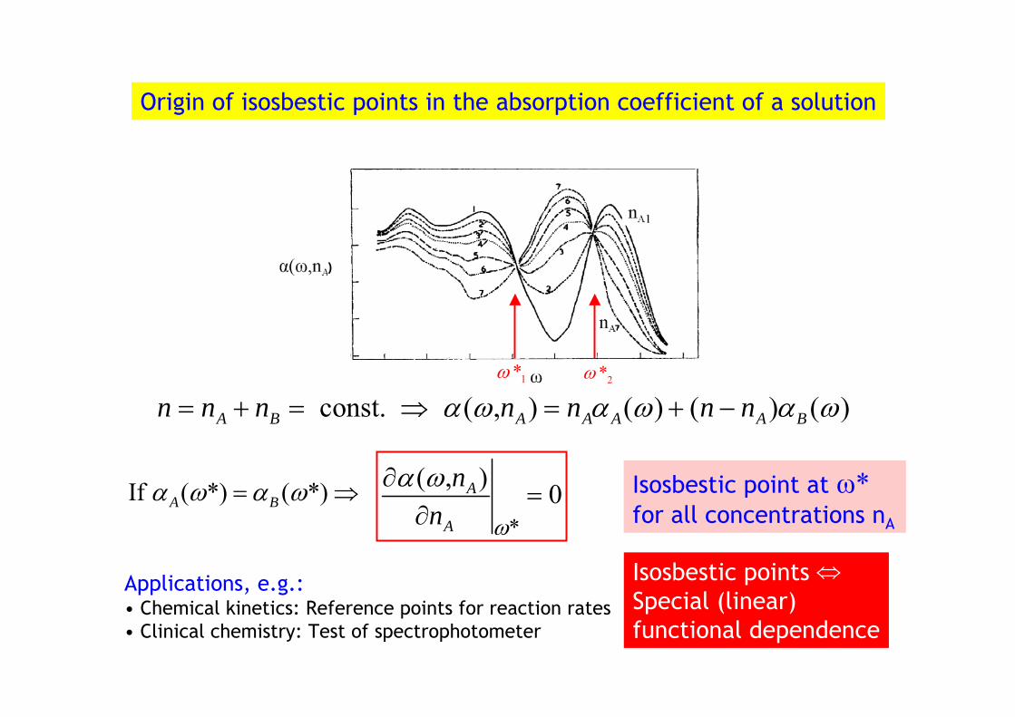
Origin of isosbestic points in the absorption coefficient of a solution

const. ( , ) ( ) ( ) ( )A B A A A A Bn n n n n n nα ω α ω α ω= + = ⇒ = + −

)

Applications, e.g.:• Chemical kinetics: Reference points for reaction rates• Clinical chemistry: Test of spectrophotometer

Isosbestic point at ω*for all concentrations nA

If ( *) ( *)A Bα ω α ω= ⇒*

( , ) 0A

A

nn ω

α ω∂=

∂

1*ω 2*ω

Isosbestic points Special (linear) functional dependence

⇔

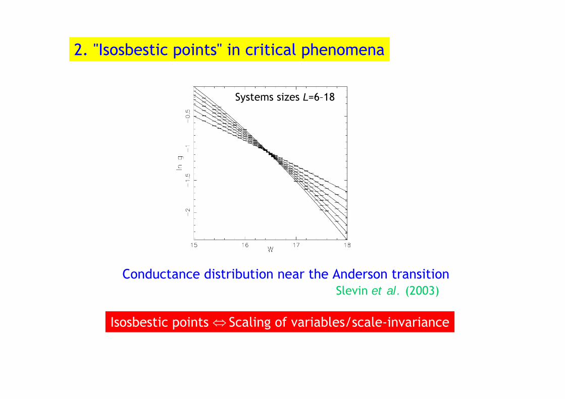
Systems sizes L=6–18

Conductance distribution near the Anderson transitionSlevin et al. (2003)

2. "Isosbestic points" in critical phenomena

Isosbestic points Scaling of variables/scale-invariance⇔

Approximate isosbestic points

a) Thermodynamic quantities

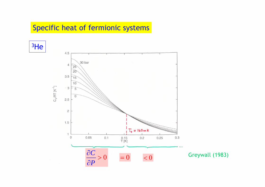
Greywall (1983)

3He

Specific heat of fermionic systems

0= 0<0CP∂∂

>

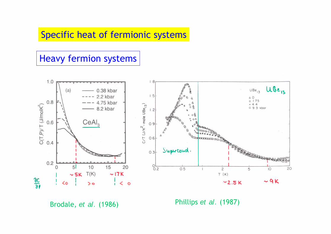
Heavy fermion systems

Brodale, et al. (1986) Phillips et al. (1987)

Specific heat of fermionic systems

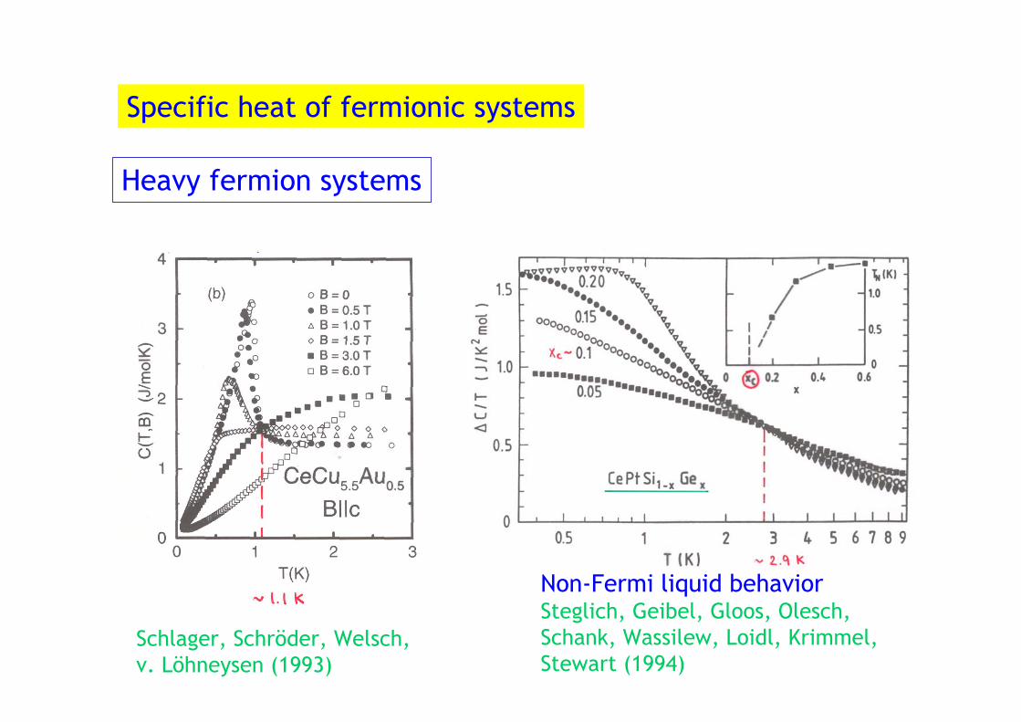
Heavy fermion systems

Schlager, Schröder, Welsch, v. Löhneysen (1993)

Non-Fermi liquid behaviorSteglich, Geibel, Gloos, Olesch,Schank, Wassilew, Loidl, Krimmel,Stewart (1994)

Specific heat of fermionic systems

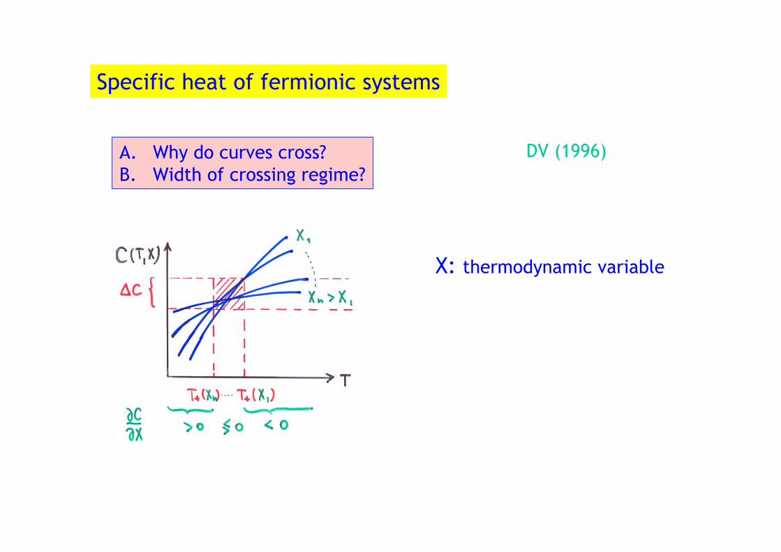
X: thermodynamic variable

DV (1996)A. Why do curves cross?B. Width of crossing regime?

Specific heat of fermionic systems

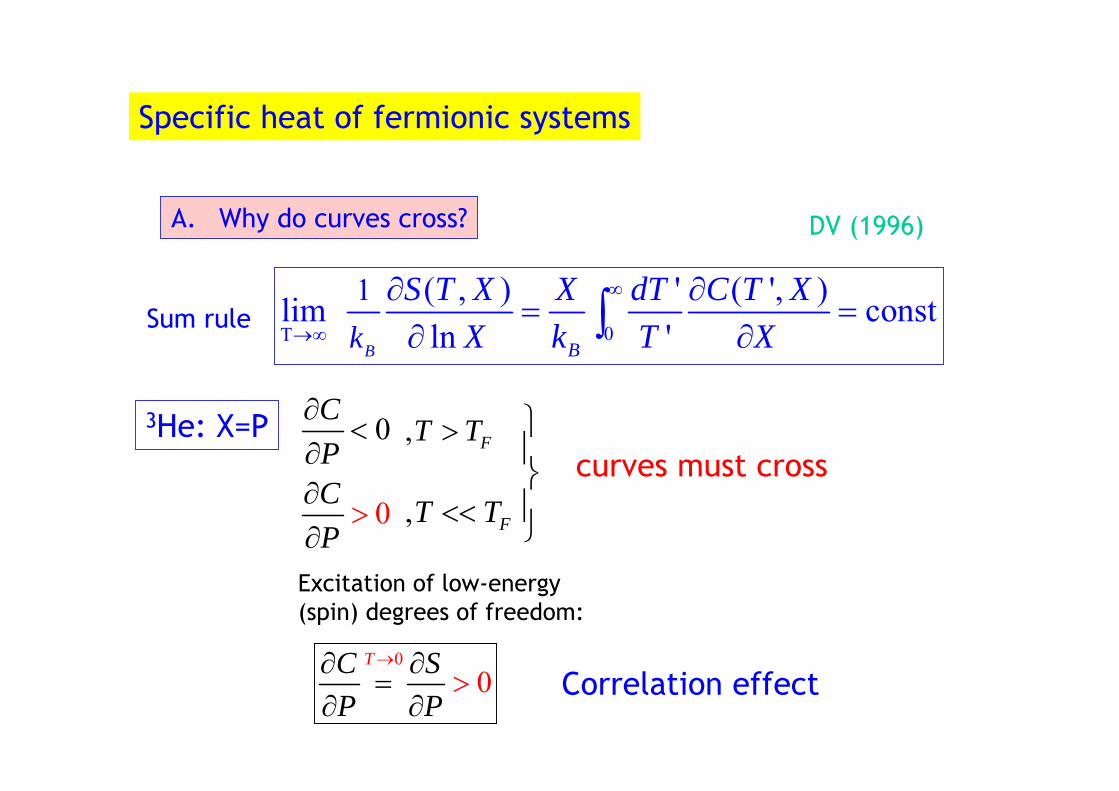
Sum rule

3He: X=P ⎫⎪⎬⎪⎭

curves must cross, FT T>

, FT T<<

0

0

CPCP

∂<

∂∂

>∂

DV (1996)

Correlation effect

Excitation of low-energy(spin) degrees of freedom:

00

TC SP P

→∂ ∂=

∂>

∂

A. Why do curves cross?

0T

1 ( , ) ' ( ', )lim constln 'B Bk

S T X X dT C T XX k T X

∞

→∞

∂ ∂= =

∂ ∂∫

Specific heat of fermionic systems

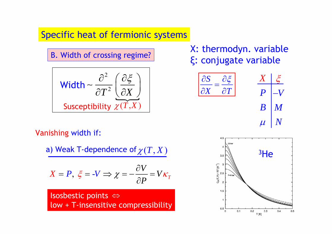
X: thermodyn. variableξ: conjugate variable

2

2

( , )T XT X

χ

ξ∂ ∂⎛ ⎞⎜ ⎟∂ ∂⎝ ⎠

∼Width

Susceptibility

Isosbestic points low + T-insensitive compressibility

⇔

B. Width of crossing regime?

SX T

ξ∂ ∂=

∂ ∂XPBμ

VMN

ξ−

Vanishing width if:

3He( , )T Xχa) Weak T-dependence of

-, TV VP

X P V χξ κ∂= = ⇒ = − =

∂

Specific heat of fermionic systems

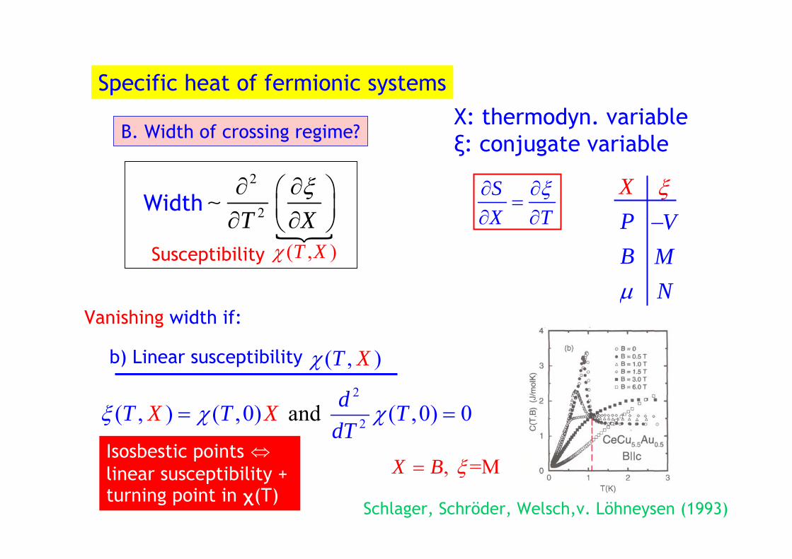
X: thermodyn. variableξ: conjugate variable

Vanishing width if:

Isosbestic points linear susceptibility + turning point in χ(T)

⇔

B. Width of crossing regime?

2

2an( , ) ( ,0) ( , 0)d 0dT T TdT

X Xξ χ χ= =

, =MX B ξ=

Schlager, Schröder, Welsch,v. Löhneysen (1993)

( , )T Xχb) Linear susceptibility

SX T

ξ∂ ∂=

∂ ∂XPBμ

VMN

ξ−

2

2

( , )T XT X

χ

ξ∂ ∂⎛ ⎞⎜ ⎟∂ ∂⎝ ⎠

∼Width

Susceptibility

Specific heat of fermionic systems

Approximate isosbestic points

b) Dynamic quantities

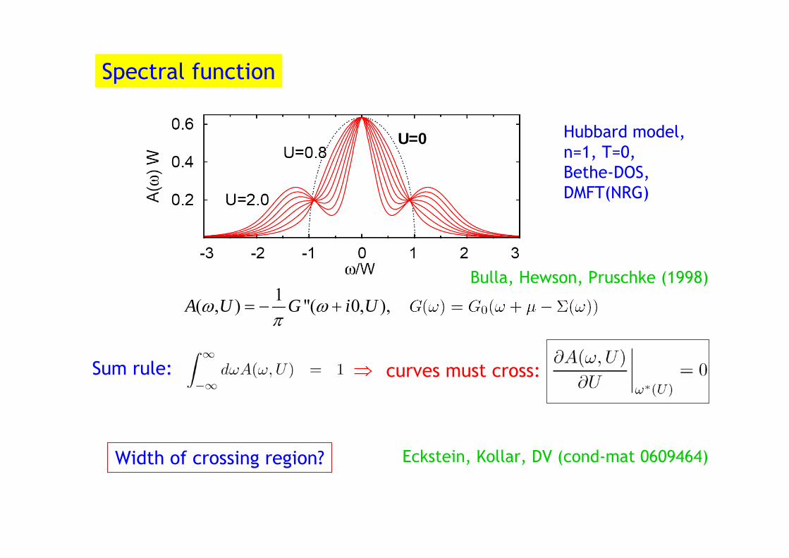
Spectral function

Hubbard model,n=1, T=0,Bethe-DOS,DMFT(NRG)

Eckstein, Kollar, DV (cond-mat 0609464)Width of crossing region?

Sum rule: curves must cross:⇒

1( , ) ''( 0, ),A U G i Uω ωπ

= − +

U=0

Bulla, Hewson, Pruschke (1998)

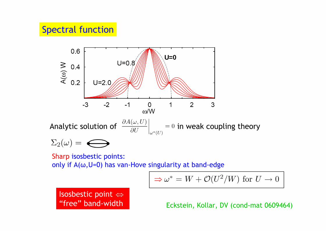
Spectral function

Eckstein, Kollar, DV (cond-mat 0609464)

Analytic solution of in weak coupling theory

Sharp isosbestic points: only if A(ω,U=0) has van-Hove singularity at band-edge

⇒

Isosbestic point “free” band-width

⇔

U=0

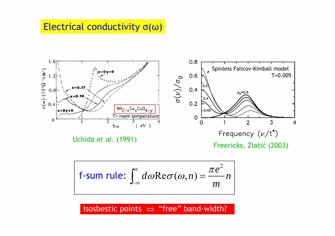
Electrical conductivity σ(ω)

Uchida et al. (1991)

T= room temperature

Spinless Falicov-Kimball model T=0.005

Freericks, Zlatić (2003)

f-sum rule:2

Re ( , ) ed n nmπω σ ω

∞

−∞=∫

Isosbestic points “free” band-width?⇔

II. Kinks in the effective electronic dispersion

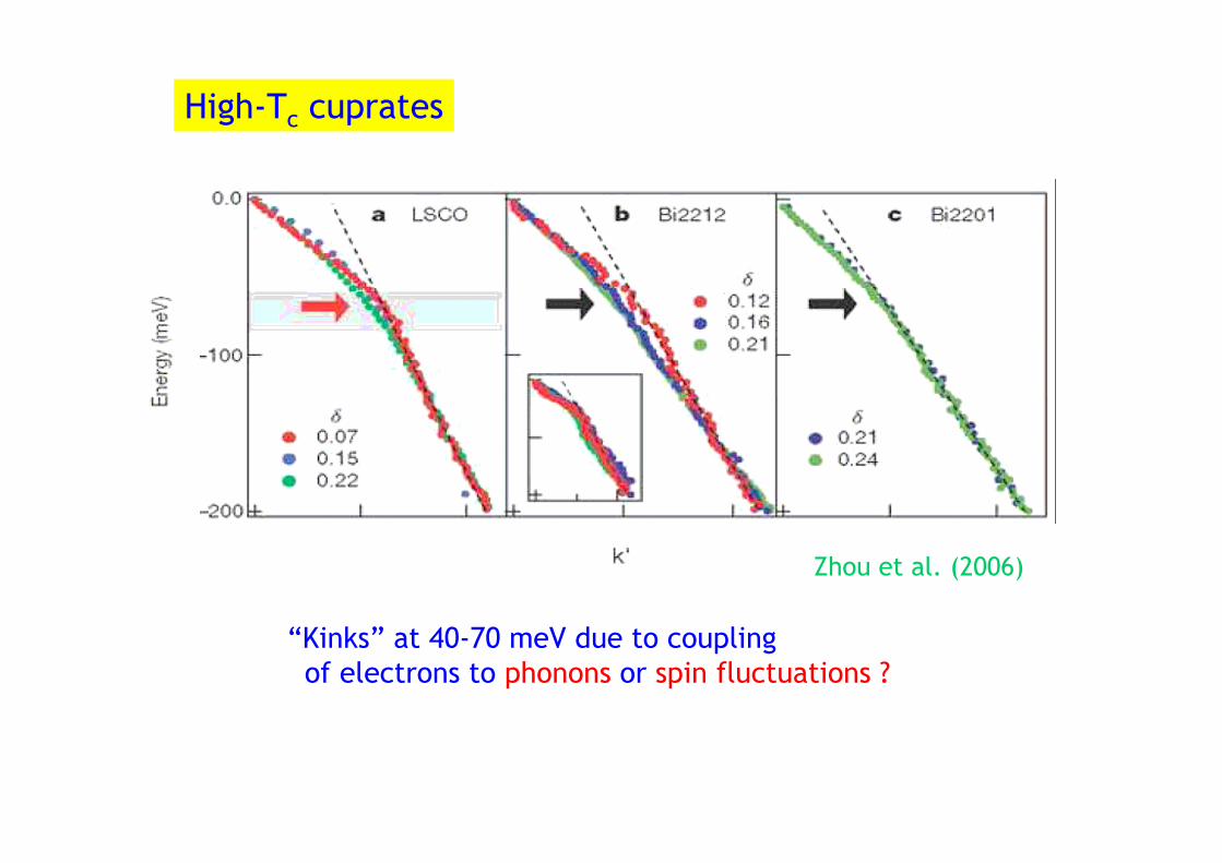
“Kinks” at 40-70 meV due to coupling of electrons to phonons or spin fluctuations ?

High-Tc cuprates

Zhou et al. (2006)

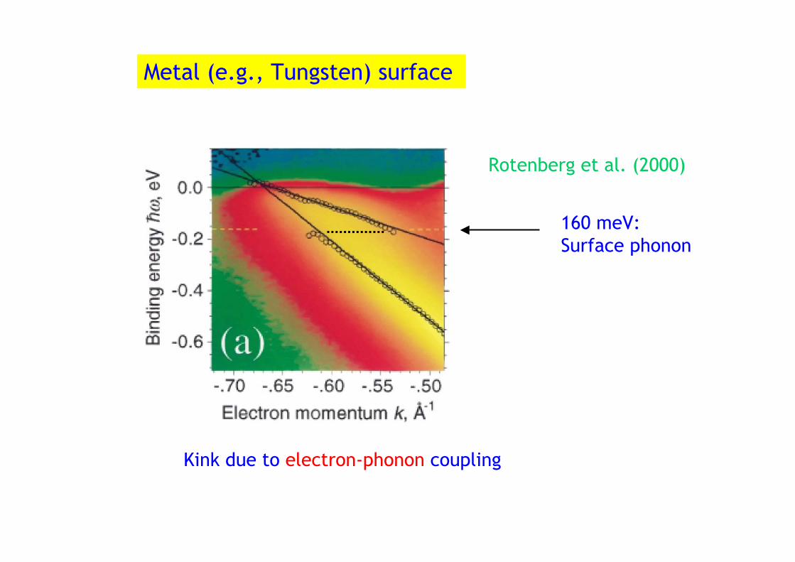
Metal (e.g., Tungsten) surface

160 meV:Surface phonon

Rotenberg et al. (2000)

Kink due to electron-phonon coupling

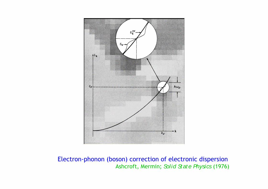
Electron-phonon (boson) correction of electronic dispersionAshcroft, Mermin; Solid State Physics (1976)

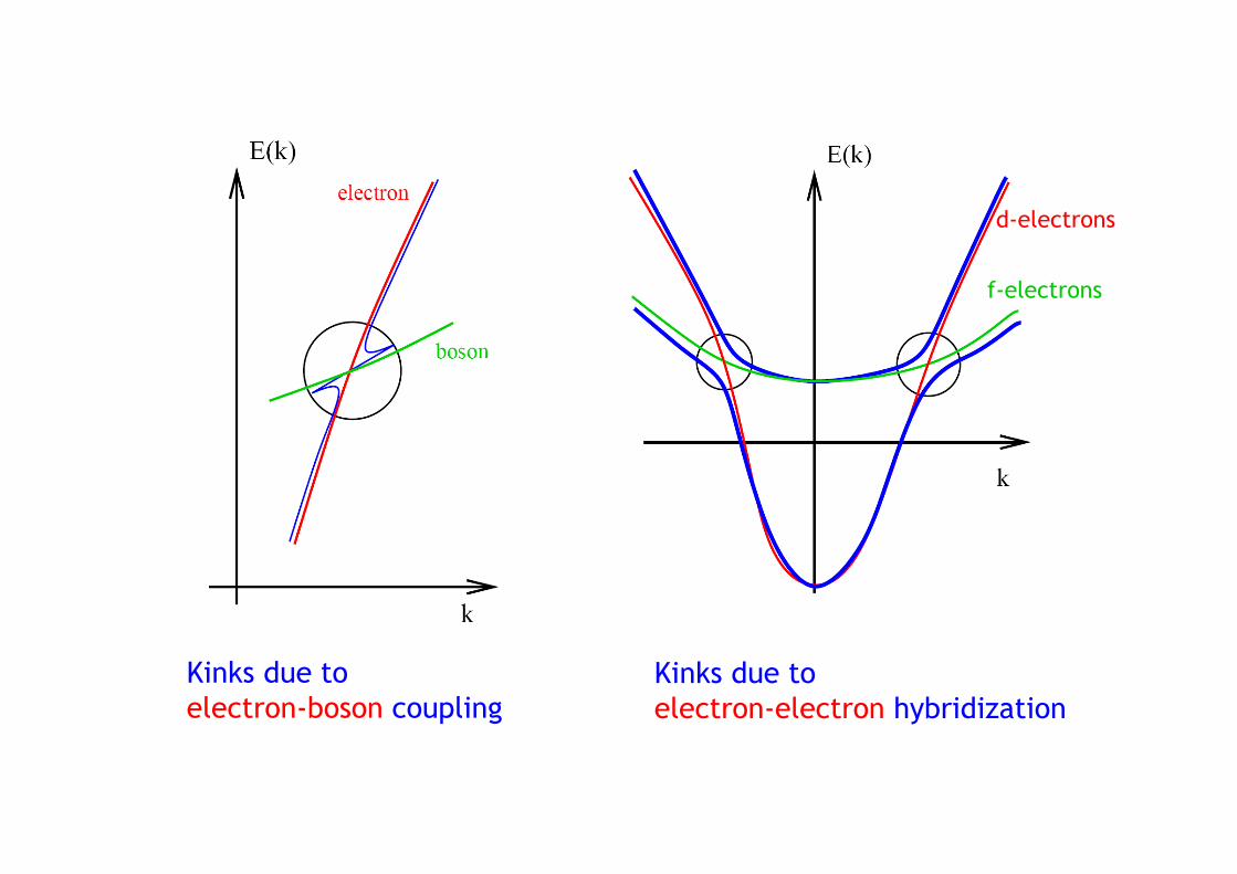
Kinks due to electron-boson coupling

Kinks due to electron-electron hybridization

f-electrons

d-electrons

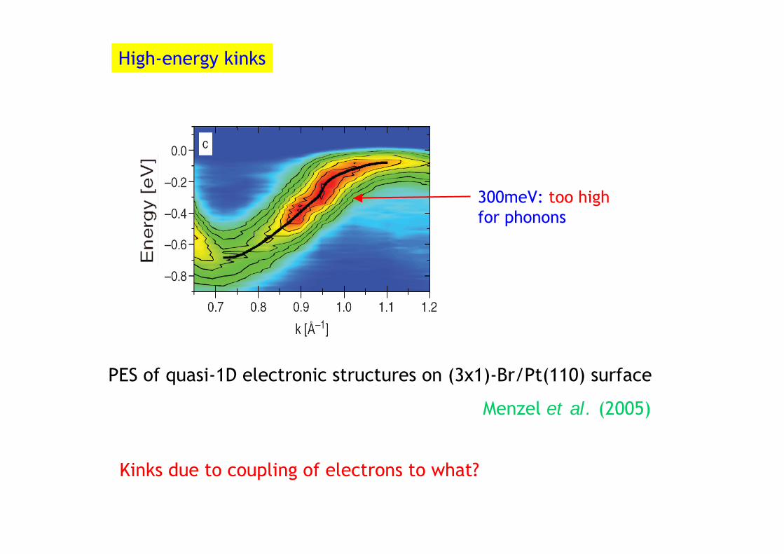
PES of quasi-1D electronic structures on (3x1)-Br/Pt(110) surface

Menzel et al. (2005)

300meV: too high for phonons

High-energy kinks

Kinks due to coupling of electrons to what?

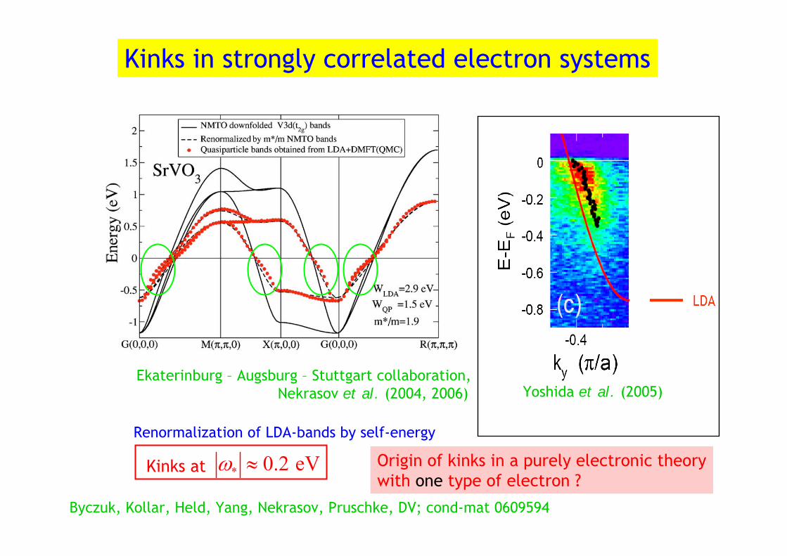
Kinks in strongly correlated electron systems

Yoshida et al. (2005)Ekaterinburg – Augsburg – Stuttgart collaboration,

Nekrasov et al. (2004, 2006)

Renormalization of LDA-bands by self-energy

* 0.2 eVω ≈Kinks at Origin of kinks in a purely electronic theorywith one type of electron ?

Byczuk, Kollar, Held, Yang, Nekrasov, Pruschke, DV; cond-mat 0609594

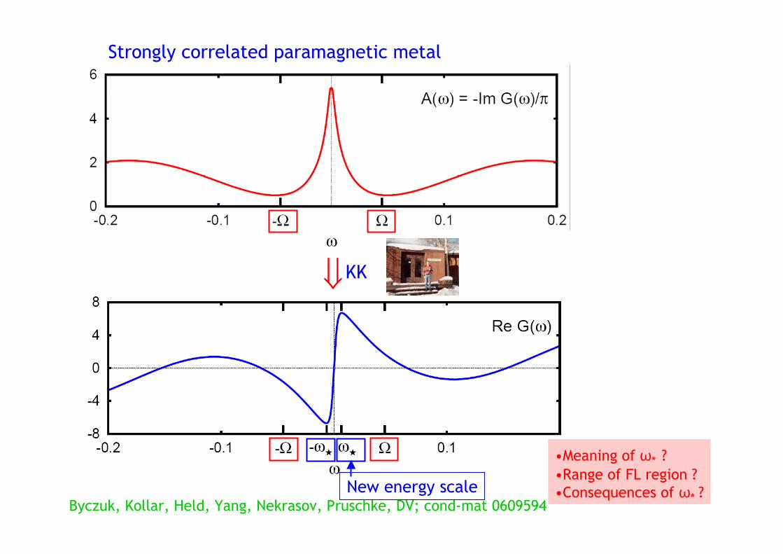
Strongly correlated paramagnetic metal

Byczuk, Kollar, Held, Yang, Nekrasov, Pruschke, DV; cond-mat 0609594

⇓KK

New energy scale

•Meaning of ω* ? •Range of FL region ? •Consequences of ω* ?

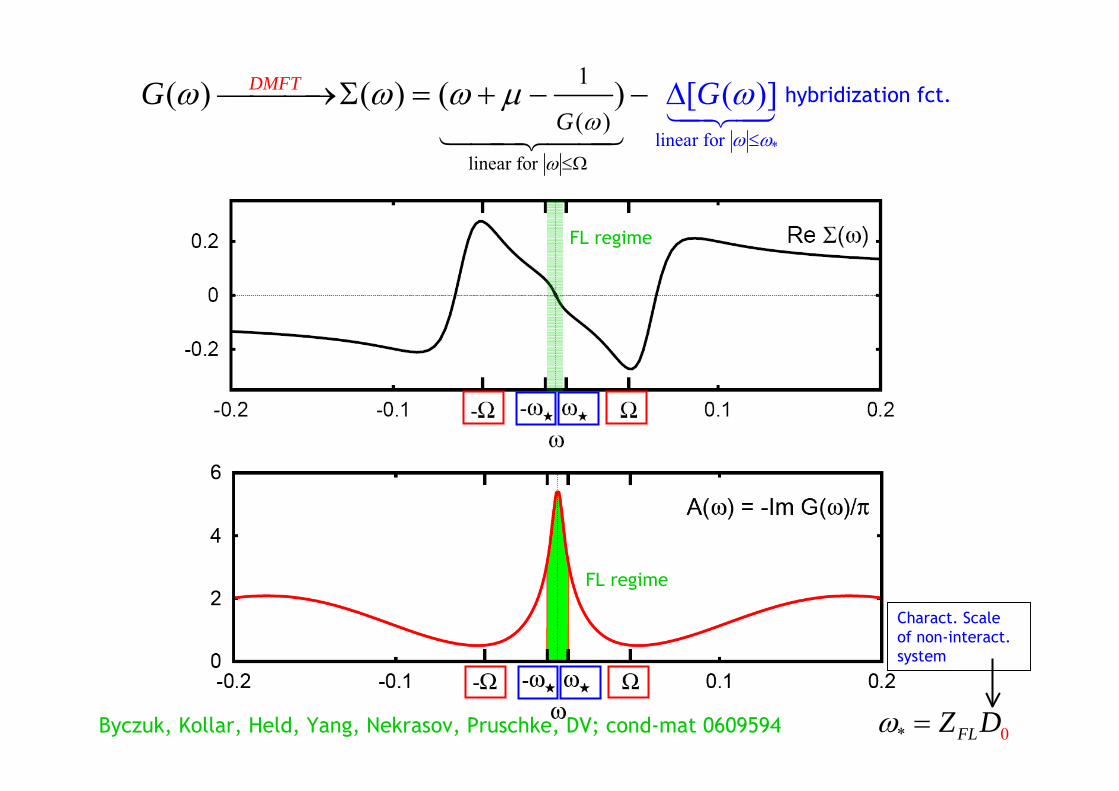
*linear flinear for

or

1

( )( ) ( [ ( ]) ( ))DMFT

GG G

ωω ω

ωω ω ω ωμ

≤Ω≤

⎯⎯⎯→Σ = − − Δ+ hybridization fct.

FL regime

FL regime

Byczuk, Kollar, Held, Yang, Nekrasov, Pruschke, DV; cond-mat 0609594 0* FLZ Dω =

Charact. Scaleof non-interact. system

analyt. given by Z + non-interact. quantities

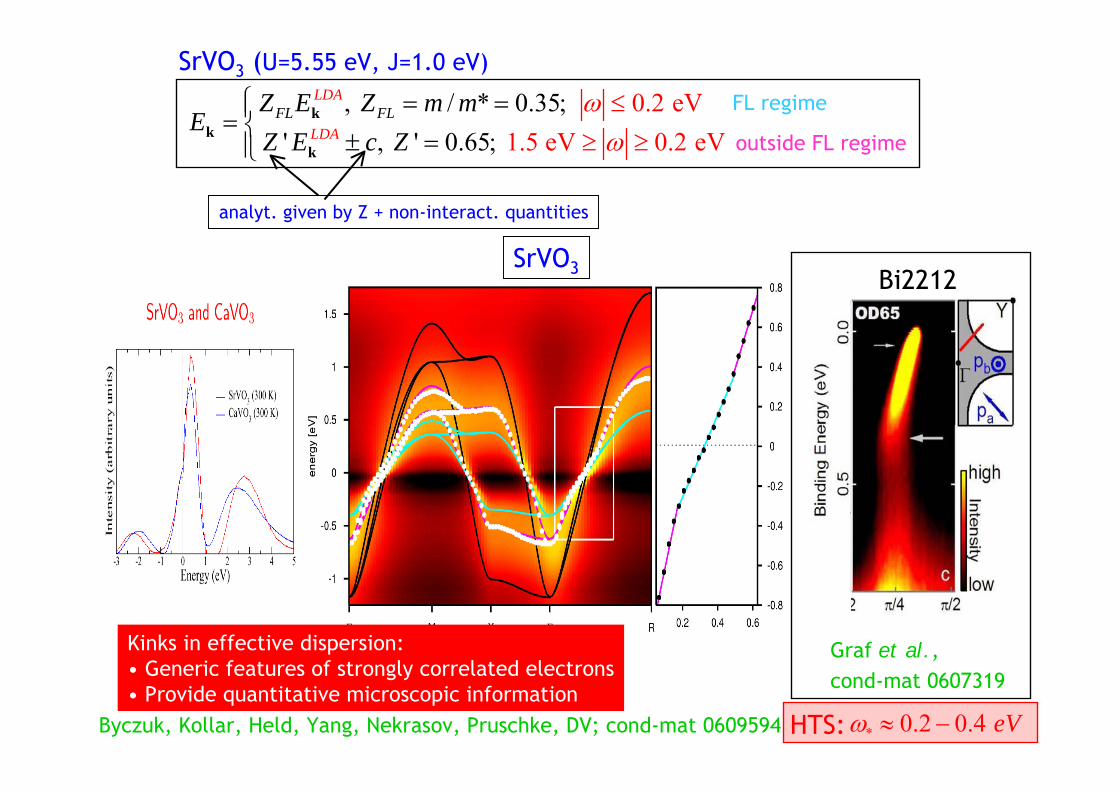
0.2 eV , / * 0.35; ' , ' 0.65; 1.5 eV 0.2 e V

LDA

LDAFL FLZ E Z m m

EZ E c Z

ωω

⎧ = =⎪= ⎨ ± =⎪⎩

≤≥ ≥

kk

k

FL regime

outside FL regime

SrVO3 (U=5.55 eV, J=1.0 eV)

SrVO3

Kinks in effective dispersion: • Generic features of strongly correlated electrons• Provide quantitative microscopic information

HTS: * 0.2 0.4 eVω ≈ −Byczuk, Kollar, Held, Yang, Nekrasov, Pruschke, DV; cond-mat 0609594

Graf et al., cond-mat 0607319

Bi2212