Isogenies and endomorphism rings of elliptic curves - ECC ...ecc2011.loria.fr/slides/summerschool-robert.pdf · Isogenies on elliptic curves—Definitions4/ 66 Notations We fix a

Isogenies and endomorphism rings of elliptic curvesECC Summer School

Damien Robert

Microsoft Research

15/09/2011 (Nancy)

— 2 / 66

Outline

1 Isogenies on elliptic curves

2 Endomorphisms

3 Supersingular elliptic curves

4 Abelian varieties

5 References

Isogenies on elliptic curves — 3 / 66

Outline

1 Isogenies on elliptic curvesDefinitionsCryptographic applications of isogeniesIsomorphisms and twistsAlgorithms for computing isogenies

2 Endomorphisms


4 Abelian varieties

5 References

Isogenies on elliptic curves — Definitions 4 / 66

Notations

We fix a perfect field k. Since our aim is cryptographic applications of ellipticcurves, most of the time k will be a finite field.An elliptic curve E is a smooth complete curve of genus 1 with a base point 0E .This base point uniquely determine a structure of algebraic group on E .If k is a finite field, every smooth complete curve of genus 1 has a rational point,so is an elliptic curve.An elliptic curve E/Fq over a finite field of characteristic p is said to besupersingular if #E[p] = {0}. In this case #E[pn] = {0} for all n. Otherwise,#E[pn] = pn for all n, and E is said to be ordinary.


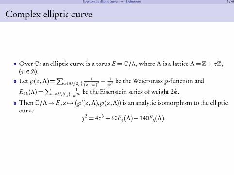
Complex elliptic curve

Over C: an elliptic curve is a torus E =C/Λ, where Λ is a lattice Λ=Z+τZ,(τ �H).Let ℘(z,Λ) =

∑

w�Λ\{0E }1

(z−w)2− 1

w2 be the Weierstrass ℘-function and

E2k (Λ) =∑

w�Λ\{0E }1

w2k be the Eisenstein series of weight 2k.

ThenC/Λ→ E , z 7→ (℘′(z,Λ),℘(z ,Λ)) is an analytic isomorphism to the ellipticcurve

y2 = 4x3− 60E4(Λ)− 140E6(Λ).


Isogenies between elliptic curves

Definition

An isogeny is a (non trivial) algebraic map f : E1→ E2 between two elliptic curvessuch that f (P +Q) = f (P )+ f (Q) for all geometric points P,Q � E1.

Example

If E is an elliptic curve, the multiplication by [m] is an isogeny.If E : y2 = x3+ ax + b is an elliptic curve defined over a finite field Fq ofcharacteristic p, the Frobenius E → E (p), (x, y) 7→ (x p , y p ) is an isogeny.Let E be the elliptic curve y2 = x3+ x over F17. Let f be the mapf (x, y) = (x, 4y). Is f an isogeny?

Remark

Isogenies are surjectives. In particular, if E is ordinary, any isogenous curve to E is alsoordinary.


Isogenies and algebraic maps

Theorem

An algebraic map f : E1→ E2 is an isogeny if and only if f (0E1) = f (0E2

)

Proof.

Over C: a bit of work on analytic functions.

Corollary

An algebraic map between two elliptic curves is eithertrivial (i.e. constant)or the composition of a translation with an isogeny.


Equivalent isogenies

Two isogenies f1 : E1→ E2 and f2 : E ′1→ E ′2 are equivalent if the following diagram commutes:

E1 E2

E ′1 E ′2

f1

f2

∼ ∼

Let E1 : y2 = x3+ 4x + 2 and E2 : y2 = x3+ 8x + 7 be two elliptic curves over F17.

Let f1 : E1→ E1 be the isogeny given by

(x9 − x8 + 8x7 − 2x6 − 6x5 + 5x4 + x3 − 4x2 + 2

x8 − x7 + 2x6 − 5x5 + 7x4 + 4x3 − 8x2 + 3x − 2,

x12y + 7x11y + 8x10y − 2x9y + 6x8y + 5x7y + 8x6y + 2x5y + 7x4y − 6x3y − 7x2y + 5xy + 4y

x12 + 7x11 − 3x10 + 7x9 − 2x8 + 2x7 − 4x6 − 6x5 − 8x4 − 5x3 + 3x2 + 6x + 3)

Let f2 : E1→ E2 be the isogeny given by

(x9 + 3x7 − 5x6 + 4x5 − 5x4 − 3x3 + 6x2 − 2x + 6

−8x8 + 8x6 + 8x5 + 4x4 − 4x3 − 5x2 − 3x + 1,

x12y + 3x10y − 2x9y − 5x8y − 8x7y − 4x6y − x5y − 7x4y + x3y − 6x2y − 2xy − 6y

−7x12 + 2x10 + 2x9 − 8x8 − 2x7 − 8x6 − x5 − 5x4 + 8x3 − 2x2 + 4x + 1)

Is f1 equivalent to f2?


Equivalent isogenies

f1 and f2 have the same degrees. But E1 = E2!But they have the same j -invariant ( j = 4), so they are isomorphics.

We could compose f2 with an isomorphism E2∼→ E1 and test if it is equal to f1.

But even if the curves were equal, we could still compose with automorphisms.So we have to construct “canonical” isogenies from f1 and f2.Easier way: compute the kernels!

ker f1 = x4+ 8x2+ 8x + 6

ker f2 = x4+ 8x3+ 3x2+ 16x + 7

The kernel are different, hence the isogenies are not the same. (SinceAut(E1) = {±1}).Exercice: prove that f1 is equivalent to the multiplication by 3.


Isogenies and kernels

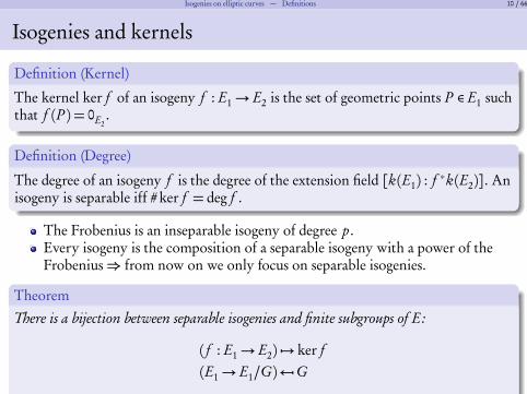
Definition (Kernel)

The kernel ker f of an isogeny f : E1→ E2 is the set of geometric points P � E1 suchthat f (P ) = 0E2

.

Definition (Degree)

The degree of an isogeny f is the degree of the extension field [k(E1) : f ∗k(E2)]. Anisogeny is separable iff #ker f = deg f .

The Frobenius is an inseparable isogeny of degree p.Every isogeny is the composition of a separable isogeny with a power of theFrobenius⇒ from now on we only focus on separable isogenies.

Theorem

There is a bijection between separable isogenies and finite subgroups of E:

( f : E1→ E2) 7→ ker f(E1→ E1/G) 7→G


Isogenies and multiplications

If H ⊂G are finite subgroups of E , then the isogeny E → E/G splits asE → E/H → (E/H )/(G/H ).In particular, for every (separable) isogeny f : E → E ′, there exists acontragredient isogeny f ′ : E ′→ E such that f ′ ◦ f = [m], where m is theexponent of ker f .

We can also identify f ′ as the dual isogeny f of f (if m = deg f ):

0 K E E ′ 0

0 E E ′ K 0

f

f∼ ∼


Algorithms for manipulating isogenies

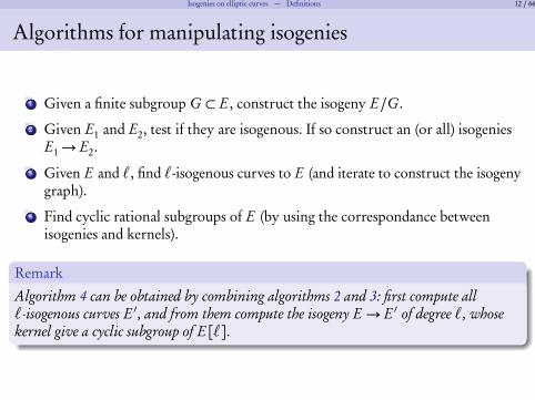
1 Given a finite subgroup G ⊂ E , construct the isogeny E/G.

2 Given E1 and E2, test if they are isogenous. If so construct an (or all) isogeniesE1→ E2.

3 Given E and ℓ, find ℓ-isogenous curves to E (and iterate to construct the isogenygraph).

4 Find cyclic rational subgroups of E (by using the correspondance betweenisogenies and kernels).

Remark

Algorithm 4 can be obtained by combining algorithms 2 and 3: first compute allℓ-isogenous curves E ′, and from them compute the isogeny E → E ′ of degree ℓ, whosekernel give a cyclic subgroup of E[ℓ].

Isogenies on elliptic curves — Cryptographic applications of isogenies 13 / 66

Destructive cryptographic applications

An isogeny f : E1→ E2 transports the DLP problem from E1 to E2. This can beused to attack the DLP on E1 if there is a weak curve on its isogeny class (and anefficient way to compute an isogeny to it).

Example

extend attacks using Weil descent [GHS02] (remember Vanessa’s talk!)

Transfert the DLP from the Jacobian of an hyperelliptic curve of genus 3 to the Jacobianof a quartic curve [Smi09].


Constructive cryptographic applications

One can recover informations on the elliptic curve E modulo ℓ by working overthe ℓ-torsion.But by computing isogenies, one can work over a cyclic subgroup of cardinal ℓinstead.Since thus a subgroup is of degree ℓ, whereas the full ℓ-torsion is of degree ℓ2, wecan work faster over it.

Example

The SEA point counting algorithm [Sch95; Mor95; Elk97] (go to François’ talk for moredetails).

The CRT algorithms to compute class polynomials [Sut09; ES10].

The CRT algorithms to compute modular polynomials [BLS09].


Further applications of isogenies

Splitting the multiplication using isogenies can improve the arithmetic(remember Laurent’s talk) [DIK06; Gau07].The isogeny graph of a supersingular elliptic curve can be used to constructsecure hash functions [CLG09].Construct public key cryptosystems by hiding vulnerable curves by an isogeny(the trapdoor) [Tes06], or by encoding informations in the isogeny graph[RS06].Take isogenies to reduce the impact of side channel attacks [Sma03].Construct a normal basis of a finite field [CL09].Improve the discrete logarithm in F∗q by finding a smoothness basis invariant byautomorphisms [CL08].

Isogenies on elliptic curves — Isomorphisms and twists 16 / 66

Class of isomorphisms of elliptic curves

Every elliptic curve has a Weierstrass equation:

y2+ a1xy + a3y = x3+ a2x2+ a4x + a6 (1)

with the discriminant∆E =−b2b8− 8b3− 27b2+ 9b2b4b6 = 0.(Here b2 = a2

1 + 4a2 , b4 = 2a4+ a1a3 , b6 = a23 + 4a6 ,

b8 = a21a6+ 4a2a6− a1a3a4+ a2a2

3 − a24 ).

The j -invariant of E is

jE =(b 2

2 − 24b4)3

∆E

Theorem

Two elliptic curves E and E ′ are isomorphics over k if and only if jE = jE ′ .


The case of a finite field of characteristic p > 3

We can always write the Weierstrass equation as

y2 = x3+ ax + b .

The discriminant is −16(4a3+ 27b 2).The j -invariant is

jE = 17284a3

4a3+ 27b 2.


Isomorphisms

The isomorphisms (over k) of isomorphisms of elliptic curves in Weierstrassform are given by the maps

(x, y) 7→ (u2x + r, u3y + u2 s x + t )

for u, r, s , t � k, u = 0.If we restrict to elliptic curves of the form y2 = x3+ ax + b then s = t = 0.

Proposition

Let E/Fq and E ′/Fq be two ordinary elliptic curves such that jE = jE ′ . Then

E ≃ E ′ over Fq

⇔ E and E ′ are isogenous over Fq

⇔ #E = #E ′.


Twists

A twist of an elliptic curve E/Fq is an elliptic curve E ′/Fq isomorphic to E over

Fq but not over Fq .

Every elliptic curve E : y2 = x3+ ax + b has a quadratic twist

E ′ : δy2 = x3+ ax + b

for any non square δ � Fq . E and E ′ are isomorphic over F2q .

If E/Fq is an ordinary elliptic curve with jE � {0,1728} then the only twist of Eis the quadratic twist. If jE = 1728, then E admits 4 twists. If jE = 0, then Eadmits 6 twists.

Isogenies on elliptic curves — Algorithms for computing isogenies 20 / 66

When are two elliptic curves isogenous?

Theorem (Tate)

Two elliptic curves over Fq are isogenous if and only if they have the same cardinal.

Proof.

If E and E ′ are isogenous, they have the same cardinal: use the dual isogeny andlook at the action of the Frobenius on E[ℓ] for ℓ not dividing the degree of theisogeny.The reciprocal is a theorem of Tate.


Isogenies between two elliptic curves

In this slide, E1/Fq and E2/Fq are ordinary elliptic curves over Fq .

If E1 and E2 are isogenous, then any isogeny over Fq is in fact Fq -rational.

If f : E1→ E2 is an isogeny over Fq of prime degree, then there exist twists E ′1and E ′2 of E1 and E2 such that f descends to an Fq -rational isogeny f : E ′1→ E ′2.

Either HomFq(E1, E2) = {0} or HomFq

(E1, E2) is a free Z-module of rank 2.


Computing explicit isogenies

If E1 and E2 are two elliptic curves given by Weierstrass equations, a morphismof curve f : E1→ E2 is of the form

f (x, y) = (R1(x, y), R2(x, y))

where R1 and R2 are rational functions, whose degree in y is less than 2 (usingthe equation of the curve E1).If f is an isogeny, f (−P ) =− f (P ). If car k > 3 so we can assume that E1 and E2are given by reduced Weierstrass forms, this mean that R1 depends only on x,and R2 is y time a rational function depending only on x.Let wE = d x/2y be the canonical differential. Then f ∗wE ′ = cwE , with c in k.This show that f is of the form

f (x, y) =

g (x)

h(x), cy�

g (x)

h(x)

�′!

.

h(x) give (the x coordinates of the points in) the kernel of f (if we take it primeto g ).If c = 1, we say that f is normalized.


Isogeny from the kernel

Remark

Every isogeny is a composition of a multiplication by [m] and an isogeny with cyclickernel (we could even further reduce to a composition with cyclic kernels of prime orders).

Let E/k be an elliptic curve. Let G = ⟨P ⟩ be a rational finite subgroup of E . Wewant to construct the isogeny E → E/G.We need to find the Weierstrass coordinates X ,Y on k(E/G). Butk(E/G) = k(E)G are the rational functions on E invariants under translation bya point of G.Moreover the Weierstrass coordinates x and y on E are characterized (up toisomorphism) by

v0E(x) =−2 vP (x)¾ 0 if P = 0E

v0E(y) =−3 vP (y)¾ 0 if P = 0E

y2/x3(0E ) = 1


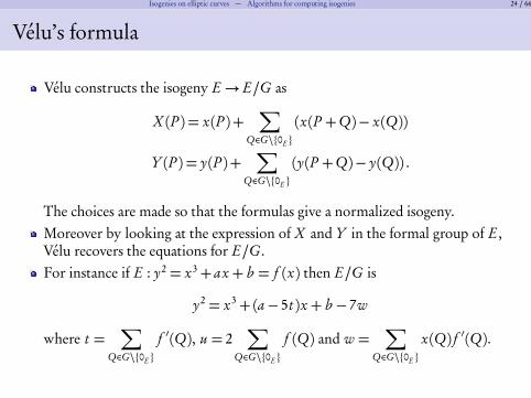
Vélu’s formula

Vélu constructs the isogeny E → E/G as

X (P ) = x(P )+∑

Q�G\{0E }(x(P +Q)− x(Q))

Y (P ) = y(P )+∑

Q�G\{0E }(y(P +Q)− y(Q)) .

The choices are made so that the formulas give a normalized isogeny.Moreover by looking at the expression of X and Y in the formal group of E ,Vélu recovers the equations for E/G.For instance if E : y2 = x3+ ax + b = f (x) then E/G is

y2 = x3+(a− 5t )x + b − 7w

where t =∑

Q�G\{0E }f ′(Q), u = 2

∑

Q�G\{0E }f (Q) and w =

∑

Q�G\{0E }x(Q) f ′(Q).


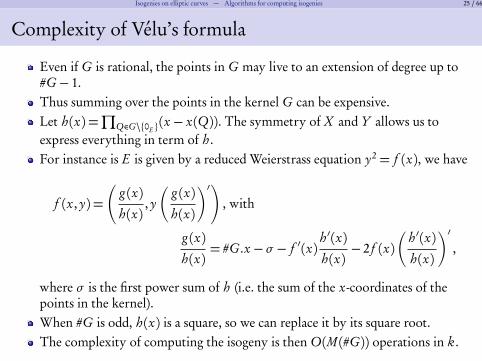
Complexity of Vélu’s formula

Even if G is rational, the points in G may live to an extension of degree up to#G− 1.Thus summing over the points in the kernel G can be expensive.Let h(x) =

∏

Q�G\{0E }(x − x(Q)). The symmetry of X and Y allows us toexpress everything in term of h.For instance is E is given by a reduced Weierstrass equation y2 = f (x), we have

f (x, y) =

g (x)

h(x), y�

g (x)

h(x)

�′!

, with

g (x)

h(x)= #G.x −σ − f ′(x)

h ′(x)h(x)− 2 f (x)

�

h ′(x)h(x)

�′,

where σ is the first power sum of h (i.e. the sum of the x-coordinates of thepoints in the kernel).When #G is odd, h(x) is a square, so we can replace it by its square root.The complexity of computing the isogeny is then O(M (#G)) operations in k.


Computing isogenous curves from E

Let E be an elliptic curve and ℓ a prime number. We want to compute allℓ-isogenous elliptic curves to E .Easy! Compute the rational cyclic subgroups of E[ℓ] and apply Vélu’s formulas.These subgroups can be obtained as factors of the ℓ-division polynomial∏

Q�E[ℓ]\{0E }(x − x(Q)).

But the division polynomial has degree (ℓ2− 1)/2 (if ℓ odd), and factorizing itwill cost O(ℓ3.63). We only want to compute isogenies of degree ℓ. Can we dobetter?


Modular polynomials

Here k = k.

Definition (Modular polynomial)

The modular polynomial ϕℓ(x, y) �Z[x, y] is a bivariate polynomial such thatϕℓ(x, y) = 0⇔ x = j (E) and y = j (E ′) with E and E ′ ℓ-isogeneous.

Roots of ϕℓ( j (E), .)⇔ elliptic curves ℓ-isogeneous to E .There are ℓ+ 1= #P1(Fℓ) such roots if ℓ is prime.ϕℓ is symmetric.The height of ϕℓ grows as O(ℓ).


Rational roots of the modular polynomials

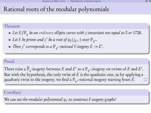
Theorem

Let E/Fq be an ordinary elliptic curve with j -invariant not equal to 0 or 1728.

Let ℓ be prime and j ′ be a root of ϕℓ( jE , ·) over Fqn .

Then j ′ corresponds to a Fqn -rational ℓ-isogeny E → E ′.

Proof.

There exist a Fq -isogeny between E and E ′ so a Fqn -isogeny on twists of E and E ′.But with the hypothesis, the only twist of E is the quadratic one, so by applying aquadratic twist to the isogeny, we find a Fqn -rational isogeny starting from E .

Corollary

We can use the modular polynomial ϕℓ to construct ℓ-isogeny graphs!


Computing the modular polynomial

1 The complex analytic method: if we see τ 7→ j (τ) and τ 7→ j (τ/ℓ) as a modularfunctions on H; then ϕℓ(·, j ) is the minimal polynomial of j (·/ℓ) in C( j ). Onecan then recover the polynomial by computing the Fourrier coefficients of j andj (·/ℓ) with high precision.

2 The CRT method: use Vélu’s formulas to compute ϕℓ mod p for small p andthe CRT to recover the full modular polynomial.

Remark

Using asymptotically fast algorithms, both algorithms are quasilinear in the size ℓ3

of ϕℓ, so the computations are memory bounded. But the CRT algorithm allow tocompute the specialization ϕℓ( j , ·) � Fp[x] directly and is the faster in practice.

To reduce the size of the coefficients, one use a different modular function in X ∗0 (ℓ)than j (τ/ℓ).


Finding an isogeny between two isogenous elliptic curves

Let E and E ′ be ℓ-isogenous abelian varieties (we can check that ϕℓ( jE , jE ′) = 0.We want to compute the isogeny f : E → E ′.The explicit forms of isogenies are given by Vélu’s formula, which givenormalized isogenies. We first need to normalize E ′.Over C, the equation of the normalized curve E ′ is given by the Eisenstein seriesE4(ℓτ) and E6(ℓτ). We have j ′(ℓτ)/ j (ℓτ) =−E6(τ)/E4(τ). By differencing themodular polynomial, we recover the differential logarithms.We obtain that from E : y2 = x3+ ax + b , a normalized model of jE ′ is given bythe Weierstrass equation

y2 = x3+Ax +B

where A=− 148

J 2

jE ′ ( jE ′−1728) , B =− 1864

J 3

j 2E ′ ( jE ′−1728)

and J =− 18ℓ

baϕ′(X )ℓ( jE , jE ′ )

ϕ′(Y )ℓ( jE , jE ′ )

jE .

Remark

E2(τ) is the differential logarithm of the discriminant. Similar methods allow to recoverE2(ℓτ), and from it σ =

∑

P�K\{0E } x(K).


Finding the isogeny between the normalized models (I:Stark’s method)

We need to find the rational function I (x) = g (x)/h(x) giving the isogenyf : (x, y) 7→ (I (x), yI ′(x)) between E and E ′.Over C the coordinates of the elliptic curve are given by the elliptic functions:x =℘(z) and y =℘′(z).We have to find I such that ℘E ′(z) = I ◦℘E (z).Stark’s idea is to develop ℘E ′ as a continuous fraction in ℘E , and approximate Ias pn/qn .

This algorithm is quasi-quadratic ( eO(ℓ2)).


Finding the isogeny between the normalized models (II:Elkie’s method)

We need to find the rational function I (x) = g (x)/h(x) giving the isogenyf : (x, y) 7→ (I (x), yI ′(x)) between E and E ′.Plugging f into the equation of E ′ shows that I satisfy the differential equation

(x3+ ax + b )I ′(x)2 = I (x)3+AI (x)+B .

Using an asymptotically fast algorithm to solve this equation yields I (x) in timequasi-linear ( eO(ℓ)).Knowing σ gains a logarithmic factor.


Finding an isogeny between two isogenous elliptic curves(the case of small characteristic)

The preceding algorithm needs p > 8ℓ− 5 to solve the differential equation.

Idea in small characteristic: lift the curves toQq by taking lifts ejE and ejE ′ such

that ϕℓ(ejE , ejE ′) = 0 and apply the preceding algorithm.Even if E ′ is normalized, we need the modular polynomial to lift E ′ andnormalize the lift.


Finding an isogeny: total complexity

To summarize, we have the following algorithm to find an isogeny from E in largecharacteristic:

Algorithm ([BMS+08])

1 Compute ϕℓ (cost eO(ℓ3))2 Specialize on jE to obtain ϕℓ(X , jE ) (cost eO(ℓ2 log q))3 Find a root jE ′ of ϕℓ(X , jE ) to obtain the j -invariant of a ℓ-isogenous curve E ′ (costeO(ℓ log2 q)).

4 Compute the normalized model for E ′ (cost eO(ℓ2 log q)).5 Solve the differential equation (cost eO(ℓ log q)).


Finding an isogeny: total complexity

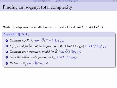
With the adaptation in small characteristic still of total cost eO(ℓ3+ ℓ log2 q):

Algorithm ([LS08])

1 Compute ϕℓ(X , jE ) (cost eO(ℓ3+ ℓ2 log q)).2 Lift jE and find a root ejE ′ in precision O(1+ log2 ℓ/ log q) (cost eO(ℓ log2 q)).3 Compute the normalized model for eE ′ (cost eO(ℓ2 log q)).4 Solve the differential equation inQq (cost eO(ℓ log q)).

5 Reduce in Fq (cost eO(ℓ log q)).


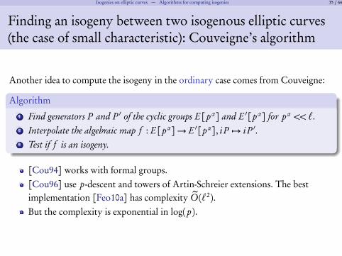
Finding an isogeny between two isogenous elliptic curves(the case of small characteristic): Couveigne’s algorithm

Another idea to compute the isogeny in the ordinary case comes from Couveigne:

Algorithm

1 Find generators P and P ′ of the cyclic groups E[pα] and E ′[pα] for pα << ℓ.2 Interpolate the algebraic map f : E[pα]→ E ′[pα], i P 7→ i P ′.3 Test if f is an isogeny.

[Cou94] works with formal groups.[Cou96] use p-descent and towers of Artin-Schreier extensions. The bestimplementation [Feo10a] has complexity eO(ℓ2).But the complexity is exponential in log(p).


Other algorithms to compute the isogeny

Lercier for p = 2: solve the differential equation using linear algebra. CosteO(ℓ3 log q) operations, in practice the fastest for p = 2.

Joux and Lercier: lift inQq with precision O(ℓ). Cost eO(ℓ2(1+ ℓ/p) log q);useful for the intermediate case p ≈ log q .When the degree ℓ is not known but only bounded by L. The naive method is toapply one of the above algorithm for all ℓ≤ L. This increase the cost by adegree 1 in L. However, Couveigne’s algorithm can be adapted to stay in eO(L2)[Feo10b].Subexponential algorithms for computing isogenies of large degree [JS10;CJS10].

Endomorphisms — 37 / 66

Outline


2 EndomorphismsDefinitionThe type of endomorphism ringsEndomorphisms and isogeniesComputing the endomorphism ring and applications


4 Abelian varieties

5 References

Endomorphisms — Definition 38 / 66

The characteristic polynomial of the Frobenius

From now on k will represent a finite field: k = Fq .

There exist a unique polynomial χπ such that for every n prime to thecharacteristic p, χπ mod n is the characteristic polynomial of the action of theFrobenius π on E[n] (here π= FrFq

).

We have χπ(π) = 0, and #E = χπ(1).We have χπ =X 2− tX + q where the trace t is such that |t |¶ 2pq (Hasse).


The endomorphism ring

Definition

If E1 and E2 are elliptic curves, we note Homk (E1, E2) the Z-module of allk-morphisms from E1 to E2. The endomorphism ring Endk (E) is thenEndk (E) =Homk (E , E).

We note End0k (E) = Endk (E)⊗ZQ the endomorphism fraction ring.

Remark

Every non nul element of Homk (E1, E2) is an isogeny (possibly non separable).

End0k (E1) is a division algebra, and Endk (E1) is an order in it.

If Homk (E1, E2) = 0, then End0k (E1) = End0

k (E2) and Homk (E1, E2) is a freeZ-module of the same rank as Endk (E1).

If E is the isogeny class of E, End0k (E) does not depend on the curve E � E .

Endk (E) is either commutative of rank 2, or an order of rank 4 in a quaternionalgebra.


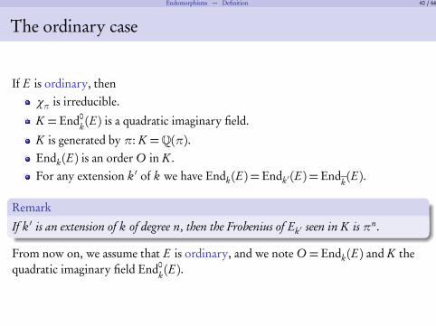
The ordinary case

If E is ordinary, thenχπ is irreducible.

K = End0k (E) is a quadratic imaginary field.

K is generated by π: K =Q(π).Endk (E) is an order O in K .For any extension k ′ of k we have Endk (E) = Endk ′(E) = Endk (E).

Remark

If k ′ is an extension of k of degree n, then the Frobenius of Ek ′ seen in K is πn .

From now on, we assume that E is ordinary, and we note O = Endk (E) and K thequadratic imaginary field End0

k (E).


Automorphisms and twist

The automorphisms of E are the inversible elements in O = End E .All inversible elements are roots of unity.We usually have O∗ = {±1} except in the following exceptions:

1 jE = 1728 ( p = 2,3), in this case O is the maximal order inQ(i) and #O∗ = 4;2 jE = 0 ( p = 2,3), in this case O is the maximal order inQ(ip3) and #O∗ = 6;3 jE = 0 ( p = 3), in this case E is supersingular and #O∗ = 12;4 jE = 0 ( p = 2), in this case E is supersingular and #O∗ = 24.

The Frobenius π �K characterizes the isogeny class of E (Tate). A twistedisogeny class will correspond to a Frobenius π′ =π, where there exist n withπn =π′n . This give a bijection between the twisted isogeny class and the roots ofunity in K .More generally, there is a bijection between O∗ and the twists of E .

Endomorphisms — The type of endomorphism rings 42 / 66

Reduction and lifting (see Marco’s talk)

Let O be an order in a imaginary quadratic field K . Then they are hO (the classnumber of O) elliptic curves overQ with endomorphism ring O. They aredefined over the ray class field HO of O.If p -∆O , p is a prime of good reduction. Let p be a prime above p in HO . If p isinert in K , Ep is supersingular. If p splits, Ep is ordinary, and its endomorphismring is the minimal order containing O of index prime to p.Reciprocally, if E/Fq is an ordinary elliptic curve, the couple (E ,End(E)) can belifted overQq .

Corollary

If E/Fq is an ordinary elliptic curve, then End(E) is an order in K =Q(π) ofconductor prime to p. For every order O of K such that Z[π]⊂O, there exist anisogenous curve whose endomorphism ring is O.Reciprocally, for every order O of discriminant a non zero square modulo p; let nbe the order of one of the prime above p in the class group of O. Then there exist an(ordinary) elliptic curve E ′ over Fqn with End(E ′) =O.

Endomorphisms — The type of endomorphism rings 43 / 66

The structure of the rational points

Theorem (Lenstra)

Let E/Fq be an ordinary elliptic curve. We have as EndFq(E)-modules

E(Fqn )≃EndFq

(E)

πn − 1

Corollary

Let a, m �Z be such that OK =Z[π−am ].

Let γE be the index of O in OK .Then E(Fq ) =Z/n1Z⊕Z/n2Z where n1 | n2 and n1n2 = #E(Fq ).

Explicitly, we have: n1 = gcd(a− 1, m/γE ).

Exercice: show that n1 | q − 1 (use the Weil pairing).

Endomorphisms — Endomorphisms and isogenies 44 / 66

Endomorphisms and isogenies

Let f : E1→ E2 be an isogeny of degree ℓ prime. Then either1 f is an ascending isogeny: O1 ⊂O2 with [O2 : O1] = ℓ;2 f is a descending isogeny: O2 ⊂O1 with [O1 : O2] = ℓ;3 f is an horizontal isogeny: O1 =O2.

The horizontal case can only happen when O1 is maximal locally in ℓ:(O1)ℓ = (OK )ℓ.Let ker f be the kernel of f . Let O f ⊂O1 be the subring (of index ℓ) of isogeniesfixing ker f . Then f induce an injection O f ,→O2.

If ψ �O∗1 is an automorphism, then either ψ fixes ker f and descends to anautomorphism of O2, or ψ induce an isogeny equivalent to f .


Isogeny graph: the local picture

Let E be an ordinary elliptic curve with endomorphism ring O, and ℓ = p be aprime.We note∆ the discriminant of OK , and∆π = t 2− 4 p the discriminant of χπ.We have∆π = γ

2∆, where γ is the conductor of Z[π]⊂OK .We note ν the ℓ-adic valuation of γ , and νE the ℓ-adic valuation of the conductorγE of O ⊂OK .


Isogeny graph: horizontal isogenies

If ν = 0, then every ℓ-isogeny is horizontal, and there are 1+ ∆ℓ

such isogeny. Moreprecisely:

1 If ℓ splits in O. In this case ∆π is a non zero square mod ℓ, and the Frobenius

acts on E[ℓ] as�

λ 00 µ

�

where the two eigenvalues λ and µ are distinct. The modular

polynomial splits into irreducible factors of degree 1, 1, r , . . . , r where r is the order ofλ/µ � Fℓ. There are 2 horizontal isogenies.

2 If ℓ is inert in O. Then∆π is not a square modulo ℓ. The two eigenvalues λ and µare conjugate in Fℓ2 \Fℓ. The modular polynomial splits as irreducible factors of degreer , where r is the smallest number such that λr � Fℓ (or equivalently such that πr actslike a scalar on E[ℓ]). There are no horizontal isogenies.

3 If ℓ is ramified in O. Then∆π ≡ 0 mod ℓ. In this case π acts on E[ℓ] as�

λ 10 λ

�

.

The modular polynomial splits into two irreducible factors of degree 1 and ℓ. There isone horizontal isogeny.


Isogeny graph: vertical isogenies

If ν = 0. ThenIf νE = 0, that is if Oℓ = (OK )ℓ. There are 1+ ∆

ℓhorizontal isogenies, and ℓ− ∆

ℓdescending isogenies (that is ℓ− 1, ℓ+ 1 or ℓ whether ℓ splits, is inert or isramified in OK ).If 0< νE < ν , there is one ascending isogeny, and ℓ-descending ones.If νE = ν , that is Oℓ =Z[π]ℓ, there is only one ascending isogeny.

In the first two cases, π acts as a scalar on E[ℓ] (and the modular polynomial splits completely), while in

the last case π acts as�

λ 10 λ

�

(and the modular polynomial splits into two irreducible factors of degree 1

and ℓ).


Isogeny graph: graphic interpretation of the local picture

The isogeny graph looks like a volcano [FM02]:


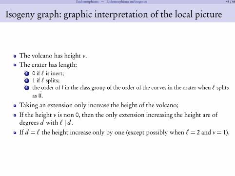
Isogeny graph: graphic interpretation of the local picture

The volcano has height ν .The crater has length:

1 0 if ℓ is inert;2 1 if ℓ splits;3 the order of l in the class group of the order of the curves in the crater when ℓ splits

as ll.

Taking an extension only increase the height of the volcano;If the height ν is non 0, then the only extension increasing the height are ofdegrees d with ℓ | d .If d = ℓ the height increase only by one (except possibly when ℓ= 2 and ν = 1).


The structure of the ℓ∞-torsion in the volcano

If E is on the floor, then E[ℓ∞](Fq ) is cyclic: E[ℓ∞](Fq ) =Z/ℓmZ (possiblym = 0).If E is on level α < m/2 above the floor, then E[ℓ∞](Fq ) =Z/ℓα⊕Z/ℓm−α.If E is on level α≥ m/2, then m is even and E[ℓ∞](Fq ) =Z/ℓm/2⊕Z/ℓm/2.

0 E[ℓ∞](Fq ) =Z/ℓm/2Z⊕Z/ℓm/2Z

1 E[ℓ∞](Fq ) =Z/ℓm/2Z⊕Z/ℓm/2Z

ν − 2 E[ℓ∞](Fq ) =Z/ℓ2Z⊕Z/ℓm−2Z

ν − 1 E[ℓ∞](Fq ) =Z/ℓZ⊕Z/ℓm−1Z

ν E[ℓ∞](Fq ) =Z/ℓmZ


The global structure

Theorem (Complex multiplication)

Let E be an elliptic curve with endomorphism ring O. Then the set of horizontal isogeniesform a principal homogeneous space under the class group of O.

This yield the following global picture (courtesy of Gaetan Bisson):

`1`2

OQ(π)

Z[π,π]

O`2O`1

O`1`2O`2

1

`1`2

Endomorphisms — Computing the endomorphism ring and applications 51 / 66

Finding the endomorphism ring

Locally: for each ℓ | γ , follow 3 paths in the ℓ-volcano. The first path reachingthe floor give us the height of the curve in the volcano.Since γ ≈pq , this is exponential.Globally, by using relations in the class groups of the orders. If R is a relation inCl(O) but the corresponding isogeny path is not cyclic then we know thatO ⊂ End(E). This give a subexponential algorithm (under GRH). More detailswill be given in Gaetan’s talk next week.

Endomorphisms — Computing the endomorphism ring and applications 52 / 66

Cryptographic applications of the endomorphism ring

It is a finer grained invariant than the number of point.It gives an idea of “where we are” in the full isogeny graph.It is used by the CRT method to compute class polynomials: from a curve in theisogeny class, we want to find a curve with maximal endomorphism ring.The cycle in the crater can be used to compute χπ mod ℓn .

Supersingular elliptic curves — 53 / 66

Outline


2 Endomorphisms


4 Abelian varieties

5 References


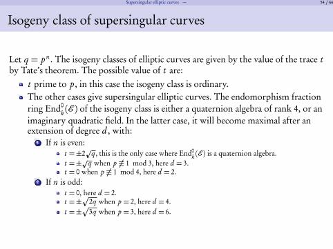
Isogeny class of supersingular curves

Let q = pn . The isogeny classes of elliptic curves are given by the value of the trace tby Tate’s theorem. The possible value of t are:

t prime to p, in this case the isogeny class is ordinary.The other cases give supersingular elliptic curves. The endomorphism fractionring End0

k (E ) of the isogeny class is either a quaternion algebra of rank 4, or animaginary quadratic field. In the latter case, it will become maximal after anextension of degree d , with:

1 If n is even:t =±2pq , this is the only case where End0

k (E ) is a quaternion algebra.t =±pq when p ≡ 1 mod 3, here d = 3.t = 0 when p ≡ 1 mod 4, here d = 2.

2 If n is odd:t = 0, here d = 2.t =±p2q when p = 2, here d = 4.t =±p3q when p = 3, here d = 6.


The commutative case

If K = End0k (E) is commutative, then χπ is irreducible and K =Q(π). Z[π] is

maximal for every ℓ = {2, p}.The endomorphism rings of the isogeny class are the orders containing Z[π]maximal at p.If O is such an order, the class group Cl(O) acts principally on the set of ellipticcurves in the isogeny class with O as ring of endomorphisms.If k ′ is such that End0

k ′(E) is maximal (i.e. a quaternion algebra), then it canhappen that some curves E ′ in the isogeny class become isomorphic to E over k ′.


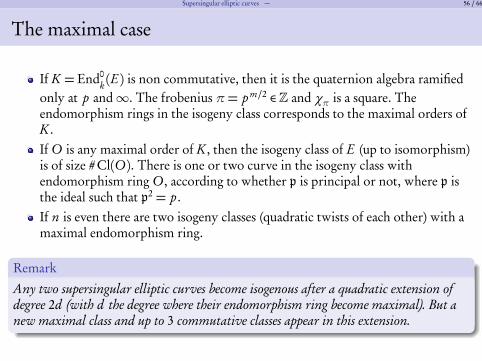
The maximal case

If K = End0k (E) is non commutative, then it is the quaternion algebra ramified

only at p and∞. The frobenius π= p m/2 �Z and χπ is a square. Theendomorphism rings in the isogeny class corresponds to the maximal orders ofK .If O is any maximal order of K , then the isogeny class of E (up to isomorphism)is of size #Cl(O). There is one or two curve in the isogeny class withendomorphism ring O, according to whether p is principal or not, where p isthe ideal such that p2 = p.If n is even there are two isogeny classes (quadratic twists of each other) with amaximal endomorphism ring.

Remark

Any two supersingular elliptic curves become isogenous after a quadratic extension ofdegree 2d (with d the degree where their endomorphism ring become maximal). But anew maximal class and up to 3 commutative classes appear in this extension.


Supersingular elliptic curves over Fp

In characteristic p, every supersingular curve is defined over Fp2 .

For every ℓ = p, the isogeny graph of supersingular curves (up to twists) overFp2 is connected. It has p/12+O(1) vertices, and diameter O(log p).

The absolute endomorphism ring Endk (E) of a supersingular curve is a maximalorder in the quaternion algebra ramified only at p and∞.There is a bijection between the set of such orders, and the set of supersingularelliptic curve (up to an action of Gal(Fp2/Fp )).

Abelian varieties — 58 / 66

Outline


2 Endomorphisms


4 Abelian varieties

5 References


Abelian varieties

Definition

An Abelian variety is a complete connected group variety over a base field k.The group law is abelian.A (separable) isogeny is a finite surjective (separable) morphism between twoAbelian varieties.

Example

Abelian varieties of dimension 1 are elliptic curves.The Jacobian of a curve of genus g is an abelian variety of dimension g .


Non absolutely simple abelian varieties

Definition

An abelian variety Ak is simple if the only subvariety of Ak are 0Akand itself.

Ak is absolutely simple if it is simple over k.

Even if an abelian variety A is ordinary, lot of funny things can happen if it is notabsolutely simple:

Not every non zero morphism is an isogeny.The endomorphism ring End0(A) = End(A)⊗Qmay not be a division algebra.We can have End0

k ′(A) = End0k (A) for extensions k ′ of k.

A can be isogenous to another abelian variety A′, isomorphic to it over anextension of k, but not isomorphic to it over k.


Decomposing abelian varieties

Theorem (Poincaré-Weil)

Every abelian variety A is isogenous to a product of simple abelian varieties A=∏

Amii .

The decomposition is entirely determined by χπA.

End0(Ai ) is a division algebra.

End0(A) =∏

Mmi(End0(Ai )).

Theorem (Tate)

H omk (A,B) is free of rank the number of common roots (with multiplicity) of χπAand

χπB.


Endomorphism rings of abelian varieties

Let A be a simple abelian variety of dimension g . Then1 χπ = me

A where mA is the minimal polynomial of the Frobenius and isirreducible.

2 End0(E) is a division algebra of centerQ(π). The type of End0(E) is entirelydetermined by π.

3 We have 2g = d e , where d is the degree of mA. End0(E) is of rank d e2.

Remark

If A is ordinary, then e = 1, χπ is irreducible and K = End0k (E) is a CM-field of

rank 2g .Moreover if A is absolutely simple, then K =Q(π) =Q(πn) for every n andEndk (A) = Endk (A).


Computing isogenies and endomorphisms

In dimension 2, one can define modular polynomials using the Igusa invariants[Gau00; Dup06; BL09]. But these are too big to compute even for ℓ¾ 3.We have an equivalent of Vélu’s formula for maximally isotropic kernels [LR10;CR11].We also have subexponentials algorithms to compute the endomorphism ring indimension 2 [Bis11b].See the package AVIsogenies [BCR10] for an implementation of isogenies andendomorphism ring computation (mostly restricted to dimension 2 for now).


Isogeny graph in genus 2: example of horizontal isogenies


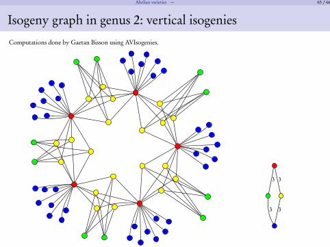
Isogeny graph in genus 2: vertical isogenies

Computations done by Gaetan Bisson using AVIsogenies.

3 3

3 3


Isogeny graph in genus 2: vertical isogenies

References — 66 / 66

Outline


2 Endomorphisms


4 Abelian varieties

5 References


Elliptic curves

For a meta look at attacks on elliptic curves using isogenies to transfert the DLP: [KKM09,Section 11.2].

Computing the modular polynomial: [Eng09a; BLS09].

Different methods to compute class fields polynomials (the best known methods use the CRT andisogenies): [Eng09b; Sut09; ES10].

Explicit isogenies in large characteristic: see [Elk92; Elk97]; and [BMS+08] for the best currentknown algorithm, with a nice history of previous methods.

Explicit isogenies in small characteristic: [JL06; LS08] for methods based on lifting, [Cou94; Cou96]for Couveigne’s algorithm. The current best implementation of Couveigne’s algorithm is in[Feo10a], a nice summary is in [Feo10b].

Some papers on SEA point counting algorithm [Sch95; Mor95; Elk97; Ler97].

About isogenies and isomorphisms descending to the base field, see [Cox89, Proposition 14.19] and[Sch95, Proposition 6.1].

See [Sil86, Chapter X, Theorem 2.2] for the equivalence between automorphisms and twists.

An algorithm to compute endomorphism ring was developed in Kohel’s thesis [Koh96]. Someextensions to supersingular curves are in [ML04; Cer04].

Developing the result of Kohel’s led to the notion of “isogeny volcano” [FM02] and improvementsof the computation of the endomorphism ring [Fou01] with applications to the CRT method tocompute class polynomials.

Finally, a subexponential algorithm is developped in [BS09; Bis11a; Bis11b].

One can also use the cycle given by the crater of the volcano to recover the trace of the Frobeniusmodulo a power of ℓ [CM94; CDM96; FM02; Fou01].


Using pairings to go up in the Volcano [IJ10]. The ℓ∞-torsion in the volcano is described there, andalso in [MMS+06].

Abelian varieties

For an introduction to abelian variety, see [Mil91]. For more informations, see [Mum70], with[Mil85; Mil86] for simplified proofs using étale cohomology, and [GM07] for a more recent account.For abelian varieties over C, see [Mum83; Mum84; Mum91] and a more recent account in [BL04].

Some nice informations on abelian varieties over finite fields (Tate’s theorem, Honda-Tate theory) see[WM71] and [Wat69] for a more complete treatment.

A description of ordinary abelian variety over a finite field is given by an equivalence of category[Del69], the link is further studied in [How95].

For algebraic theta functions, see [Mum66; Mum67a; Mum67b], and some new results in [Kem89].

Computing modular polynomials in genus 2: [Gau00; Dup06; BL09]. Computing a certain modularcorrespondance using theta functions [FLR11].

Computing isogenies in abelian varieties using theta functions [LR10; CR11].

For an introduction to the use of theta functions in cryptography (arithmetic, pairings, isogenies) see[Rob10].

Computing endomorphism ring see [EL07; FL08; Wag09; Bis11b].

Bibliography

[BL04] C. Birkenhake and H. Lange. Complex abelian varieties. Second. Vol. 302. Grundlehrender Mathematischen Wissenschaften [Fundamental Principles of Mathematical Sciences].Berlin: Springer-Verlag, 2004, pp. xii+635. ISBN: 3-540-20488-1 (cit. on p. 71).

[Bis11a] G. Bisson. “Computing endomorphism rings of elliptic curves under the GRH”. In:Journal of Mathematical Cryptology (2011). arXiv:1101.4323 (cit. on p. 70).

http://arxiv.org/abs/1101.4323


[Bis11b] G. Bisson. “Endomorphism Rings in Cryptography”. PhD thesis. 2011 (cit. on pp. 65,70, 71).

[BCR10] G. Bisson, R. Cosset, and D. Robert. “AVIsogenies (Abelian Varieties and Isogenies)”.Packet magma dédié au calcul explicite d’isogénies entre variétés abéliennes. 2010. URL:http://avisogenies.gforge.inria.fr. Licence libre (LGPLv2+), enregistré à l’APP(référence IDDN.FR.001.440011.000.R.P.2010.000.10000) (cit. on p. 65).

[BS09] G. Bisson and A. Sutherland. “Computing the endomorphism ring of an ordinaryelliptic curve over a finite field”. In: Journal of Number Theory (2009) (cit. on p. 70).

[BMS+08] A. Bostan, F. Morain, B. Salvy, and E. Schost. “Fast algorithms for computing isogeniesbetween elliptic curves”. In: Mathematics of Computation 77.263 (2008), pp. 1755–1778(cit. on pp. 34, 70).

[BL09] R. Bröker and K. Lauter. “Modular polynomials for genus 2”. In: LMS J. Comput. Math.12 (2009), pp. 326–339. ISSN: 1461-1570 (cit. on pp. 65, 71).

[BLS09] R. Bröker, K. Lauter, and A. Sutherland. Modular polynomials via isogeny volcanoes.2009. arXiv:1001.0402 (cit. on pp. 14, 70).

[Cer04] J. Cerviño. “On the correspondence between supersingular elliptic curves and maximalquaternionic orders”. In: Arxiv preprint math/0404538 (2004) (cit. on p. 70).

[CLG09] D. Charles, K. Lauter, and E. Goren. “Cryptographic hash functions from expandergraphs”. In: Journal of Cryptology 22.1 (2009), pp. 93–113. ISSN: 0933-2790 (cit. on p. 15).

[CJS10] A. Childs, D. Jao, and V. Soukharev. “Constructing elliptic curve isogenies in quantumsubexponential time”. In: Arxiv preprint arXiv:1012.4019 (2010) (cit. on p. 37).

http://avisogenies.gforge.inria.fr



[CR11] R. Cosset and D. Robert. “An algorithm for computing (ℓ,ℓ)-isogenies in polynomialtime on Jacobians of hyperelliptic curves of genus 2”. Mar. 2011. URL:http://www.normalesup.org/~robert/pro/publications/articles/niveau.pdf. HAL:hal-00578991 (cit. on pp. 65, 71).

[Cou94] J. Couveignes. “Quelques calculs en théorie des nombres”. PhD thesis. 1994 (cit. onpp. 36, 70).

[Cou96] J. Couveignes. “Computing l-isogenies using the p-torsion”. In: Algorithmic NumberTheory (1996), pp. 59–65 (cit. on pp. 36, 70).

[CDM96] J. Couveignes, L. Dewaghe, and F. Morain. Isogeny cycles and the Schoof-Elkies-Atkinalgorithm. Tech. rep. Citeseer, 1996 (cit. on p. 70).

[CL08] J. Couveignes and R. Lercier. “Galois invariant smoothness basis”. In: Algebraic geometryand its applications (2008) (cit. on p. 15).

[CL09] J. Couveignes and R. Lercier. “Elliptic periods for finite fields”. In: Finite fields and theirapplications 15.1 (2009), pp. 1–22 (cit. on p. 15).

[CM94] J. Couveignes and F. Morain. “Schoof’s algorithm and isogeny cycles”. In: AlgorithmicNumber Theory (1994), pp. 43–58 (cit. on p. 70).

[Cox89] D. Cox. Primes of the form x2+ ny2. Wiley, 1989 (cit. on p. 70).

[Del69] P. Deligne. “Variétés abéliennes ordinaires sur un corps fini”. In: InventionesMathematicae 8.3 (1969), pp. 238–243 (cit. on p. 71).

[DIK06] C. Doche, T. Icart, and D. Kohel. “Efficient scalar multiplication by isogenydecompositions”. In: Public Key Cryptography-PKC 2006 (2006), pp. 191–206 (cit. onp. 15).

[Dup06] R. Dupont. “Moyenne arithmetico-geometrique, suites de Borchardt et applications”. In:These de doctorat, Ecole polytechnique, Palaiseau (2006) (cit. on pp. 65, 71).

http://www.normalesup.org/~robert/pro/publications/articles/niveau.pdf

http://hal.archives-ouvertes.fr/hal-00578991


[EL07] K. Eisentrager and K. Lauter. “A CRT algorithm for constructing genus 2 curves overfinite fields”. In: AGCT-11 (2007) (cit. on p. 71).

[Elk92] N. Elkies. “Explicit isogenies”. In: manuscript, Boston MA (1992) (cit. on p. 70).

[Elk97] N. Elkies. “Elliptic and modular curves over finite fields and related computationalissues”. In: Computational perspectives on number theory: proceedings of a conference inhonor of AOL Atkin, September 1995, University of Illinois at Chicago. Vol. 7. AmerMathematical Society. 1997, p. 21 (cit. on pp. 14, 70).

[Eng09a] A. Enge. “Computing modular polynomials in quasi-linear time”. In: Math. Comp78.267 (2009), pp. 1809–1824 (cit. on p. 70).

[Eng09b] A. Enge. “The complexity of class polynomial computation via floating pointapproximations”. In: Mathematics of Computation 78.266 (2009), pp. 1089–1107 (cit. onp. 70).

[ES10] A. Enge and A. Sutherland. “Class invariants by the CRT method, ANTS IX:Proceedings of the Algorithmic Number Theory 9th International Symposium”. In:Lecture Notes in Computer Science 6197 (July 2010), pp. 142–156 (cit. on pp. 14, 70).

[FLR11] J.-C. Faugère, D. Lubicz, and D. Robert. “Computing modular correspondences forabelian varieties”. In: Journal of Algebra (2011). arXiv:0910.4668. URL:http://www.normalesup.org/~robert/pro/publications/articles/modular.pdf. HAL:hal-00426338. (Cit. on p. 71).

[Feo10a] L. de Feo. “Fast algorithms for computing isogenies between ordinary elliptic curves insmall characteristic”. In: Journal of Number Theory (2010) (cit. on pp. 36, 70).

[Feo10b] L. de Feo. “Algorithmes Rapides pour les Tours de Corps Finis et les Isogénies”.PhD thesis. Ecole Polytechnique X, Dec. 2010. URL:http://hal.inria.fr/tel-00547034/en (cit. on pp. 37, 70).


http://www.normalesup.org/~robert/pro/publications/articles/modular.pdf

http://hal.archives-ouvertes.fr/hal-00426338/

http://hal.inria.fr/tel-00547034/en


[Fou01] M. Fouquet. “http://www.math.jussieu.fr/ fouquet/Manuscrit.ps.gz”. PhD thesis. 2001(cit. on p. 70).

[FM02] M. Fouquet and F. Morain. “Isogeny volcanoes and the SEA algorithm”. In: AlgorithmicNumber Theory (2002), pp. 47–62 (cit. on pp. 49, 70).

[FL08] D. Freeman and K. Lauter. “Computing endomorphism rings of Jacobians of genus 2curves over finite fields”. In: Algebraic Geometry and its Applications, World Scientific(2008), pp. 29–66 (cit. on p. 71).

[GHS02] S. Galbraith, F. Hess, and N. Smart. “Extending the GHS Weil descent attack”. In:Advances in Cryptology—EUROCRYPT 2002. Springer. 2002, pp. 29–44 (cit. on p. 13).

[Gau00] P. Gaudry. “Algorithmique des courbes hyperelliptiques et applications à la cryptologie”.PhD thesis. École Polytechnique, Dec. 2000 (cit. on pp. 65, 71).

[Gau07] P. Gaudry. “Fast genus 2 arithmetic based on Theta functions”. In: Journal ofMathematical Cryptology 1.3 (2007), pp. 243–265 (cit. on p. 15).

[GM07] G. van der Geer and B. Moonen. “Abelian varieties”. In: Book in preparation (2007)(cit. on p. 71).

[How95] E. Howe. “Principally polarized ordinary abelian varieties over finite fields”. In:American Mathematical Society 347.7 (1995) (cit. on p. 71).

[IJ10] S. Ionica and A. Joux. “Pairing the volcano”. In: Algorithmic Number Theory (2010),pp. 201–218 (cit. on p. 71).

[JS10] D. Jao and V. Soukharev. “A subexponential algorithm for evaluating large degreeisogenies”. In: Algorithmic Number Theory (2010), pp. 219–233 (cit. on p. 37).

[JL06] A. Joux and R. Lercier. “Counting points on elliptic curves in medium characteristic”.Cryptology ePrint Archive, Report 2006/176. May 2006 (cit. on p. 70).


[Kem89] G. Kempf. “Linear systems on abelian varieties”. In: American Journal of Mathematics111.1 (1989), pp. 65–94 (cit. on p. 71).

[KKM09] A. Koblitz, N. Koblitz, and A. Menezes. “Elliptic curve cryptography: The serpentinecourse of a paradigm shift”. In: Journal of Number Theory (2009) (cit. on p. 70).

[Koh96] D. Kohel. “Endomorphism rings of elliptic curves over finite fields”. PhD thesis.University of California, 1996 (cit. on p. 70).

[Ler97] R. Lercier. Algorithmique des courbes elliptiques dans les corps finis. These, LIX–CNRS, juin1997. 1997. URL: http://cat.inist.fr/?cpsidt=183634 (cit. on p. 70).

[LS08] R. Lercier and T. Sirvent. “On Elkies subgroups of ℓ-torsion points in elliptic curvesdefined over a finite field.” In: Journal de théorie des nombres de Bordeaux 20.3 (2008),pp. 783–797 (cit. on pp. 35, 70).

[LR10] D. Lubicz and D. Robert. “Computing isogenies between abelian varieties”. 2010. URL:http://www.normalesup.org/~robert/pro/publications/articles/isogenies.pdf.HAL: hal-00446062 (cit. on pp. 65, 71).

[ML04] K. McMurdy and K. Lauter. “Explicit Generators for Endomorphism Rings ofSupersingular Elliptic Curves”. In: (2004) (cit. on p. 70).

[Mil85] J. Milne. “Jacobian varieties”. In: Arithmetic geometry (G. Cornell and JH Silverman, eds.)(1985), pp. 167–212 (cit. on p. 71).

[Mil86] J. Milne. “Abelian varieties”. In: Arithmetic geometry (G. Cornell and JH Silverman, eds.)(1986), pp. 103–150 (cit. on p. 71).

[Mil91] J. Milne. Abelian varieties. 1991. URL:http://www.jmilne.org/math/CourseNotes/av.html (cit. on p. 71).

http://cat.inist.fr/?cpsidt=183634

http://www.normalesup.org/~robert/pro/publications/articles/isogenies.pdf

http://hal.archives-ouvertes.fr/hal-00446062/

http://www.jmilne.org/math/CourseNotes/av.html


[MMS+06] J. Miret, R. Moreno, D. Sadornil, J. Tena, and M. Valls. “An algorithm to computevolcanoes of 2-isogenies of elliptic curves over finite fields”. In: Applied mathematics andcomputation 176.2 (2006), pp. 739–750 (cit. on p. 71).

[Mor95] F. Morain. “Calcul du nombre de points sur une courbe elliptique dans un corps fini:aspects algorithmiques”. In: J. Théor. Nombres Bordeaux 7 (1995), pp. 255–282 (cit. onpp. 14, 70).

[Mum66] D. Mumford. “On the equations defining abelian varieties. I”. In: Invent. Math. 1 (1966),pp. 287–354 (cit. on p. 71).

[Mum67a] D. Mumford. “On the equations defining abelian varieties. II”. In: Invent. Math. 3 (1967),pp. 75–135 (cit. on p. 71).

[Mum67b] D. Mumford. “On the equations defining abelian varieties. III”. In: Invent. Math. 3(1967), pp. 215–244 (cit. on p. 71).

[Mum70] D. Mumford. Abelian varieties. Tata Institute of Fundamental Research Studies inMathematics, No. 5. Published for the Tata Institute of Fundamental Research, Bombay,1970, pp. viii+242 (cit. on p. 71).

[Mum83] D. Mumford. Tata lectures on theta I. Vol. 28. Progress in Mathematics. With theassistance of C. Musili, M. Nori, E. Previato and M. Stillman. Boston, MA: BirkhäuserBoston Inc., 1983, pp. xiii+235. ISBN: 3-7643-3109-7 (cit. on p. 71).

[Mum84] D. Mumford. Tata lectures on theta II. Vol. 43. Progress in Mathematics. Jacobian thetafunctions and differential equations, With the collaboration of C. Musili, M. Nori, E.Previato, M. Stillman and H. Umemura. Boston, MA: Birkhäuser Boston Inc., 1984,pp. xiv+272. ISBN: 0-8176-3110-0 (cit. on p. 71).

[Mum91] D. Mumford. Tata lectures on theta III. Vol. 97. Progress in Mathematics. With thecollaboration of Madhav Nori and Peter Norman. Boston, MA: Birkhäuser Boston Inc.,1991, pp. viii+202. ISBN: 0-8176-3440-1 (cit. on p. 71).


[Rob10] D. Robert. “Theta functions and applications in cryptography”. PhD thesis. UniversitéHenri-Poincarré, Nancy 1, France, July 2010. URL:http://www.normalesup.org/~robert/pro/publications/academic/phd.pdf. Slideshttp://www.normalesup.org/~robert/pro/publications/slides/2010-07-phd.pdf,TEL: tel-00528942. (Cit. on p. 71).

[RS06] A. Rostovtsev and A. Stolbunov. “Public-key cryptosystem based on isogenies”. In:International Association for Cryptologic Research. Cryptology ePrint Archive (2006).eprint: http://eprint.iacr.org/2006/145 (cit. on p. 15).

[Sch95] R. Schoof. “Counting points on elliptic curves over finite fields”. In: J. Théor. NombresBordeaux 7.1 (1995), pp. 219–254 (cit. on pp. 14, 70).

[Sil86] J. H. Silverman. The arithmetic of elliptic curves. Vol. 106. Graduate Texts inMathematics. Corrected reprint of the 1986 original. New York: Springer-Verlag, 1986,pp. xii+400. ISBN: 0-387-96203-4 (cit. on p. 70).

[Sma03] N. Smart. “An analysis of Goubin’s refined power analysis attack”. In: CryptographicHardware and Embedded Systems-CHES 2003 (2003), pp. 281–290 (cit. on p. 15).

[Smi09] B. Smith. Isogenies and the Discrete Logarithm Problem in Jacobians of Genus 3Hyperelliptic Curves. Feb. 2009. arXiv:0806.2995 (cit. on p. 13).

[Sut09] A. Sutherland. “Computing Hilbert class polynomials with the Chinese remaindertheorem”. In: Mathematics of Computation (2009) (cit. on pp. 14, 70).

[Tes06] E. Teske. “An elliptic curve trapdoor system”. In: Journal of cryptology 19.1 (2006),pp. 115–133 (cit. on p. 15).

[Wag09] M. Wagner. “Über Korrespondenzen zwischen algebraischen Funktionenkörpern”.PhD thesis. Technische Universität Berlin, 2009 (cit. on p. 71).

http://www.normalesup.org/~robert/pro/publications/academic/phd.pdf

http://www.normalesup.org/~robert/pro/publications/slides/2010-07-phd.pdf

http://tel.archives-ouvertes.fr/tel-00528942

http://eprint.iacr.org/2006/145



[Wat69] W. Waterhouse. “Abelian varieties over finite fields”. In: Ann. Sci. Ecole Norm. Sup 2.4(1969), pp. 521–560 (cit. on p. 71).

[WM71] W. Waterhouse and J. Milne. “Abelian varieties over finite fields”. In: Proc. Symp. PureMath 20 (1971), pp. 53–64 (cit. on p. 71).

Documents

Isogenies and endomorphism rings of elliptic curves - ECC ...ecc2011.loria.fr/slides/summerschool-robert.pdf · Isogenies on elliptic curves—Definitions4/ 66 Notations We fix a