Embed Size (px)
Citation preview
INTERNATIONAL ATOMIC ENERGY AGENCY
INTERNATIONAL CENTRE FOR THEORETICALPHYSICS
V ' l
ISOBAR DIAGRAMS AND
INELASTIC RESONANCE PRODUCTION
G. F. WOLTERS
1965PIAZZA OBERDAN
TRIESTE

IC/65/44
INTERNATIONAL ATOMIC ENERGY AGENCY
INTERNATIONAL CENTRE FOR THEORETICAL PHYSICS
ISOBAR DIAGRAMS AND INELASTIC RESONANCE PRODUCTION*
G. F . WOLTERS * *
TRIESTE
May 1965
* To be submitted to Nuovo GirrjeiUo
** On leave of absence from the Zeeman Laboratory, University of Amsterdam,,Amsterdam, Netherlands.

SUMMARY
Experimental results for the reactions iCp-»YiV± (1385) TT ±
and a few other reactions in the few GeV energy region are discussed.
Qualitative arguments are given in favour of an interpretation of
certain non-peripheral features in terms of isobar diagrams. Sub-
sequently the reaction Kp-*pK (888) is analysed in a more rigorous
approach based on the assumption that,at large momentum trans-
fers at least, K production through an intermediate isobar is
dominant. This analysis is based on well-established conservation
laws, without making use of dynamical assumptions. As a result
it is shown that the data at 1. 5 GeV/c incident momentum are con-
sistent with the one isobar hypothesis applied in the backward hemi-5'
sphere of the overall cm-system^ for isobar spin 2 and positive
parity. The amplitudes for disintegration of the intermediate iso-
bar into the final state are approximately determined, up to some
ambiguities in phase.

ISOBAR DIAGRAMS AND INELASTIC RESONANCE PRODUCTION
1. INTRODUCTION
In the few GeV energy region the salient features observed in
K±p and JT ±p reactions, yielding final states containing one or more
resonances, are as has been noted by many authors: a marked
tendency for formation of quasi two body final states; preference
for small momentum transfers; significant structure in the resonance
disintegration angular distribution. The third feature is compatible
with disintegration of the resonance as a free particle.
Similar features have been observed in NN reactions and in pion
photoproduction from nucleons. Although the peripheral model
in suitable adaptations, meets with considerable success in account-2)
ing for these features , attention is drawn to the fact that in the
phenomenological analysis of photoproduction of pions from nucleons
in the energy region of the higher nucleon isobars, besides one meson3)
exchange diagrams isobar diagrams turned out to be necessary .
Then one might a fortiori expect that such diagrams can play a dis-
tinct role in K±N and TT±N reactions too, since here the coupling
between the incident meson and the intermediate isobars is in general
stronger than in photoproduction reactions.
In this article mainly K"p reactions will be considered in view of
examining whether known experimental data contain evidence for iso-
bar diagram contributions.
As concerns the peripheral model, it has been noticed in particular
that the third feature, mentioned above, allows one to specify to some
extent the appropriate model: the spin density matrix of the resonance
can be determined partially, and from this knowledge e. g. the ratio
of pseudoscalar meson exchange to vector meson exchange amplitudes4)follows . The application of resulting models for predicting the
resonance production angular distributions yielded some discrepancy
with the observed distributions, in particular at and above 3 GeV, the
last ones showing stronger forward peaking. This difficulty has been
removed by taking into account absorptive effects, due to competing
- 1 -
channels . Since this modification of the peripheral model does not
change the predicted resonance spin density matrix injcrucial
way, satisfactory agreement both with the observed resonance pro-
duction angular distribution and its disintegration characteristics
could be obtained. A different formulation of this modification in
terms of the K-matrix, imposing the unitarity condition on the S-
matrix, which reduces the Born terms in low partial waves, is due
to DIETZ and PILKUHN6*.
Meanwhile,it is realized that even these refined peripheral
models do not account for the observed features at all momentum
transfers in certain reactions, nor are they applicable to all re-
actions possible,e. g. in K~p collisions. Also if three or more par-
ticle final states (non-resonant background), are somehow taken into
account explicitly, such as in Dietz and Pilkuhn's model, where a
statistical treatment is applied to such states, this difficulty remains.
It is the purpose of this article to draw attention to a few such non-
peripheral features in I p reactions, and to consider the possibility of
relating these features to isobar diagrams. In Section 2 this will
be done in a rather qualitative way, whereas in Section 3 a more
detailed study follows of the reaction Kp-*pK" (888). Also here the
K production angular distribution and its disintegration angular
distribution will be predicted, and comparison with experimental
data will be made.
2. SOME EMPIRICAL REMARKS ON Kp REACTIONS
The major part of this section is devoted to the reactions
Kp- Y^ ir at 1. 5 GeV/c incident momentum (Lab). At the end of
the section some other reactions will briefly be considered.
Not all phenomena observed in the Ya production reactions7)
have been interpreted in a satisfactory way . In part,large statistical
uncertainties in the measured production angular distribution, Yi
disintegration angular distribution, A polarisation etc. obscure the
true structure. Nevertheless some typicalnonperipheral features
- 2 -
are well established experimentally. These features will be discussed
below,
The notation A to indicate the unit vector along the 3 momentum
of particle A in the overall rest system, is adopted. Sometimes A*
will be taken in another reference frame, which will then be stated
explicitly.6) *
The experiment shows some backward peaking of Yj , which
is roughly equal for the two charge states. Since one meson exchange
cannot contribute to Yi production, this is no argument in favour
of important peripheral production of Yi*+ . Actually a much more
pronounced forward peaking of the Yj* 's is observed. This effect
is most important for Y]*" ', for both charge states inclusion of
negative fourth order terms in (K[.Yi ) is necessary for the fit to the
production angular distribution . No peripheral model, with reason-
able choices of form factors, reproduces this structure . From the
density distribution in the Dalitz plot one estimates that 5 per cent
of the events in the resonance mass bands correspond to non-resonant
final states , The background amplitude appears to be too small to
account for the observed deviation of the production angular distribution
from predicted forms in a peripheral model.
A second indication for the presence of a non-peripheral production
mechanism comes from what might be called the pi(Yj ) anomaly.
The Yi"" spin alignment along the direction of motion of the incident
K-meson, K"* seen in a Yi rest system, which direction is taken as
a z-axis in that rest system, is specified by plfYj* ), measuring the
population of Jz = ± f Y-j* spin states. It is assumed that Y-,* (1385)
has spin 2 . The experiment reveals that p|(Yj*) is significantlysmaller than one for Yj* production angles, such that j (JT^Yi* )| > 0. 85.
More precisely one has pifY^* )s0.4±0.1, respectively p^(Ya*" )c±
0. 65 ±0.10 for I {KfYj* ) ]& 0. 85. The same orders of magnitude are
found when less collimated Yj*'s are also considered. (Statistics
prevented consideration of more collinated Y-j* 's : for ((KTY^)]^
0. 96 one is left with 14 Yx*+ 's and with 20 Yx*~ 's.) The anomaly
consists of a discrepancy with the expectation pj(Yi )^1 for
j (KTY;! ) (£. 0.85 if peripheral production were dominant. The exchanged
- 3 -
K would leave invariant the z-component of the baryon spin. Again
the effect appears to be too large to be due to interference with the
background amplitude. If the non-resonant Aff+ system would have
angular momentum with exclusively Jz*±j, which would be the most
favourable case for such an explanation, the background amplitude,
necessary besides one meson exchange amplitude still amounts to
40 per cent or more. The argument is further supported by the fact
that the observed Yi disintegration angular distribution in the polar
angle of A, taken in the Yj* rest system, does not show any deviation
from symmetry. Finally the argument is not invaliditated by some7) A
indications in the observed Yj disintegration angular distribution
in the azimuthal angle and in the distribution of the A polarization,
as a function of the polar angle of A, for disturbing interference
effects, since these distributions refer to quantities that entirely depend
on interference between different amplitudes and are much more sen-
sitive to disturbing interference effects.
The measured values of p^(Yi*) necessarily require orbital
angular momenta i s 2 of the Yj* ir system to be important, once9)
final state interactions are neglected . The well-known argument
that at production angles 6 and IT- 6 quasi two-body final states with
£Q<^1 have J z = ±\ for the baryon, yields this lower bound. The
result is consistent with the occurrence of fourth order terms in the
Yj production angular distribution.
On account of the properties of the Y]* production angular dis-
tribution and the alignment of the Yj* spin, discussed above, one
infers that a non-peripheral production mechanism is indeed active,
rather than assuming dominant peripheral production, and putting
the blame for the p|(Yi* ) anomaly on the account of final state inter-7)
actions . In fact a natural interpretation follows immediately if
isobar diagrams are introduced. Just as in the phenomenological8)
analysis of photo production reactions , one may think of uncrossed
and crossed Born diagrams, indicated in Figs.l .a and l.b respectively
These diagrams represent the simplest possible non-peripheral
mechanism.
- 4 -
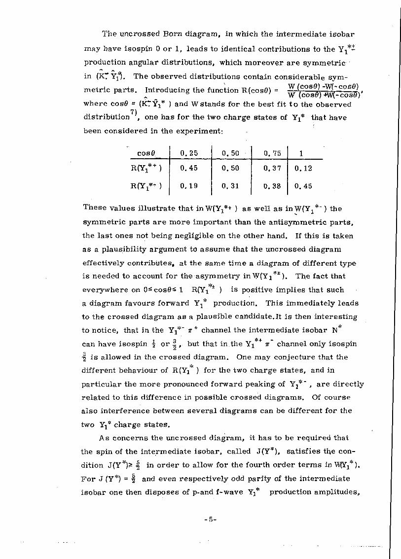
The uncrossed Born diagram, in which the intermediate isobar
may have isospin 0 or 1, leads to identical contributions to the Y^-
production angular distributions, which moreover are symmetric
in (Kf Yx*. The observed distributions contain considerable sym-
metric parts. Introducing the function R(cosG) =
where cos9 = {ICY^* ) and W Stands for the best fit to the observed7)
distribution , one has for the two charge states of Yj* that have
been considered in the experiment:
COS0
ROT!** )
RfY, - )
0.
0.
0.
25
45
19
0.
0 .
0.
50
50
31
0.
0.
0.
75
37
38
1
0.12
0.45
These values illustrate that inW(Y:,*+ ) as well as inW(Y *") the
symmetric parts are more important than the antisymmetric parts,
the last ones not being negligible on the other hand. If this is taken
as a plausibility argument to assume that the uncrossed diagram
effectively contributes, at the same time a diagram of different type
is needed to account for the asymmetry in\y(Yi**). The fact that
everywhere on O^cos0£ 1 R(Yi ) is positive implies that such
a diagram favours forward YT* production. This immediately leads
to the crossed diagram as a plausible candidate.lt is then interesting
to notice, that in the w + channel the intermediate isobar N
can have isospin | or | , but that in the Yj ir~ channel only isospin
-g is allowed in the crossed diagram. One may conjecture that the
different behaviour of R(Yi ) for the two charge states, and in
particular the more pronounced forward peaking of Yj*~ , are directly
related to this difference in possible crossed diagrams. Of course
also interference between several diagrams can be different for the
two Yj* charge states.
As concerns the uncrossed diagram, it has to be required that
the spin of the intermediate isobar, called J(Y*), satisfies the con-
dition J{Y*)£ | in order to allow for the fourth order terms in WO *).
For J (Y*) - | and even respectively odd parity of the intermediate
isobar one then disposes of p-and f-wave Yj* production amplitudes,
- 5 -
respectively d- and g-wave amplitudes, for the uncrossed diagram.
This combined with presence of crossed diagrams, which leads to
Yi*jr states without a limitation on allowed Jt-values, seems to be
sufficient to account for the observed low values of pi(Yi*±), dis-
cussed before. A comparable example, where a sole uncrossed
diagram with p- and f-wave amplitudes, yields an amount of spin
alignment which is less than half the value predicted on the basis
of one pseudoscalar meson exchange, for production angles near
0 or 7T, will be treated in Section 3.
It need hardly be emphasized that the tentative interpretation
of the salient features observed for the process considered above,
based on an isobar»»peripheral model rather than a peripheral model, is pre-
liminary. Neither the available data, nor the arguments used in
their interpretation, lead to conclusive results at present. The
type of analysis to be performed in a somewhat more quantitative
approach, is well known. An example is a recent study of some
associated production reactions at comparable energies, in which
both isobar diagrams and one meson exchange diagrams are taken
into account explicitly . Here a few general remarks on the
appropriate isobar-peripheral model are made only.
In order to obtain a manageable model one is tempted to restrict
oneself to the nearest singularities of the production amplitude.
The total CM energy being =s 2 GeV, this leads to identifying ten-
tatively the intermediate isobar in Fig.l.awith Yo* (1815), This iso-
bar probably possesses spin and parity J = | + . Also Y1 (1765)
might contribute, with T = "5 . Study of the reaction KV+YJ* TT will
enable one to determine the relative weights of the two diagrams.
In FigXb one is led to identify N* with N respectively N3* (1238)
as plausible candidates. Adjustable parameters in the isobar model
are effective coupling constant products and partial widths. Results
for these parameters will be important for comparison with pre-
dictions from symmetry schemes.
Contributions due to K* exchange cannot a priori be excluded;
at a higher energy such contributions are known to be dominant. Cf.
remarks below. Finally.as mentioned before, certain observable
- 6 -

quantities may be sensitive to the influence of non-resonant final
states.
The model will lead to predictions of the Yj* production dif-
ferential cross-section and the joint final state density matrix, as
functions of energy.
Secondly, the type of useful experimental information will thus
be: production cross-sections, production angular distributions, Y-j*
disintegration angular distributions in polar and azimuthal angle and
A polarization over the range of incident momenta 1 .3- 1. 7 GeV/c
at least. Similar data for the reaction Kn-^Yj* w will be of import-
ance. As concerns the Yj* disintegration characteristics, separation
of the Yj* sample according to some intervals of production angle
corresponding to increasing four-momentum transfer is desirable,
in order to gain better insight into the role of peripheral contributions
presumably present mainly at the smallest momentum transfers, and
of contributions from crossed isobar diagrams, presumably present
mainly at the largest momentum transfers occurring in the reaction.
A less ambitious approach consists of selecting reactions for
which the number of possible contributing diagrams is smaller than
for lCp-*Yi* IT. Evidence for isobar diagrams may then be contained
already in a smaller amount of experimental data, e. g. data for fixed
total energy, and their contributions may be studied conveniently.
As a first example f£p reactions at 3 GeV/c incident momentum
(Lab) may be mentioned. Besides final states which are definitely
produced peripherally, such as hK" ; 2Z+n;~ ; A I** ; ^ 1 ; y, rt"
and pK , also final states are observed, with smaller cross-sections,
in which the baryon moves preferably " in forward directions.
Examples are S~rr* ; ) / * - r c+ \ £ ~ K + ahd 3 " K * + 12).
Uncrossed isobar diagrams seem to be negligible at this momentum,
whereas one meson exchange is excluded. It appears therefore that
these reactions are entirely due to crossed isobar diagrams, if the
simplest possible mechanism is again preferred instead of more
complicated ones that might be invented. From this point of view
these reactions are obviously important and worth studying in great
detail both experimentally and theoretically.
- 7 -
An a priori more complicated example is provided by reactions
of the type K+p->NK*; N*K or N*K*. Here uncrossed isobar diagrams
are forbidden, if no strangeness + 1 isobar exists at least. Data at
1. 5 GeV/c incident momentum (Lab) have been analysed in a peripheral13)
model with form factors . To the author's knowledge no attempt
has been made to consider crossed isobar diagrams explicitly, in
addition to one meson exchange diagrams. Data at 3GeV/c seem to
be consistent with dominant peripheral production, with absorptive14)
effects taken into account . In view of these results and the results
for iCp reactions at this same high momentum, it thus turns out that
at 3GeV/c isobar diagrams probably are not competitive with peri-
pheral diagrams in K*p reactions. Their precise influence is un-
known.
A third example is the reaction Kp-»pK , where crossed iso-
bar diagrams are forbidden. According to the previous remark and
the discussion of the reactions Kp-»Yi TT, one may expect that K
production as indicated, at 1. 5 GeV/c, provides evidence for the
presence of intermediate isobars Yo* (1815) or Yi*(1675), besides
possibly one meson exchange. This process is therefore suitable for
examining more critically than has been done so far, if further
evidence for the "isobar-peripheral" model can be obtained, in spite
of the limited experimental data available. The following section
deals with this problem.
3 STUDY OF THE REACTION ICp^pK*" AT 1. 5 GeV/c INCIDENTMOMENTUM
The experimental results of an investigation of the reaction
ltp-*pK*"(888) at 1. 5 GeV/c incident momentum (Lab)15'16*, as
far as they are relevant for the following analysis, are recalled
here:
(a) The histogram for the K*~ production angular distribution
in the overall CM system, shown in Fig. 2. Forward K*"pro-
duction is dominant, but in addition a peak in the backward hemi-
sphere is p
and = -0.8.
sphere is present. Its maximum lies between (K. K ,.') = -Oi 6
- 8 -
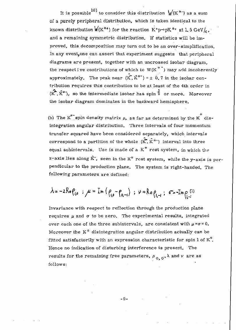
It is possible to consider this distribution \ /(K*") as a sum
of a purely peripheral distribution, which is taken identical to the
known distribution V(K*+) for the reaction K+p-»pK*+ at 1. 5 GeV/Q,
and a remaining symmetric distribution. If statistics will be im-
proved, this decomposition may turn out to be an over-simplification.
In any event,one can assert that experiment suggests, that peripheral
diagrams are present, together with an uncrossed isobar diagram,
the respective contributions of which to W(K ) may add incoherently
approximately. The peak near (K". K*~) = ± 6. 7 in the isobar con-
tribution requires this contribution to be at least of the 4th order in
(KT. K "), so the intermediate isobar has spin 2 or more, Moreover
the isobar diagram dominates in the backward hemisphere.
*- *
(b) The K spin density matrix p, as far as determined by the K dis-
integration angular distribution. Three intervals of four momentum
transfer squared have been considered separately, which intervals
correspond to a partition of the whole (K*. K*~) interval into three
equal subintervals. Use is made of a Kw rest system, in which the
z-axis lies along K", seen in the K* rest system, while the y-axis is per-
pendicular to the production plane. The system is right-handed. The
following parameters are defined:
A- -zRe f,, , p = I . (ftf- f J • „ a R. . r.-T» ft wInvariance with respect to reflection through the production plane
requires ju and cr to be zero. The experimental results, integrated
over each one of the three subintervals, are consistent with n~a~ 0.
Moreover the K* disintegration angular distribution actually can be
fitted satisfactorily with an expression characteristic for spin 1 of K*.
Hence no indication of disturbing interference is present. The
results for the remaining free parameters, p •, X and v are as
follows:
- 9 -
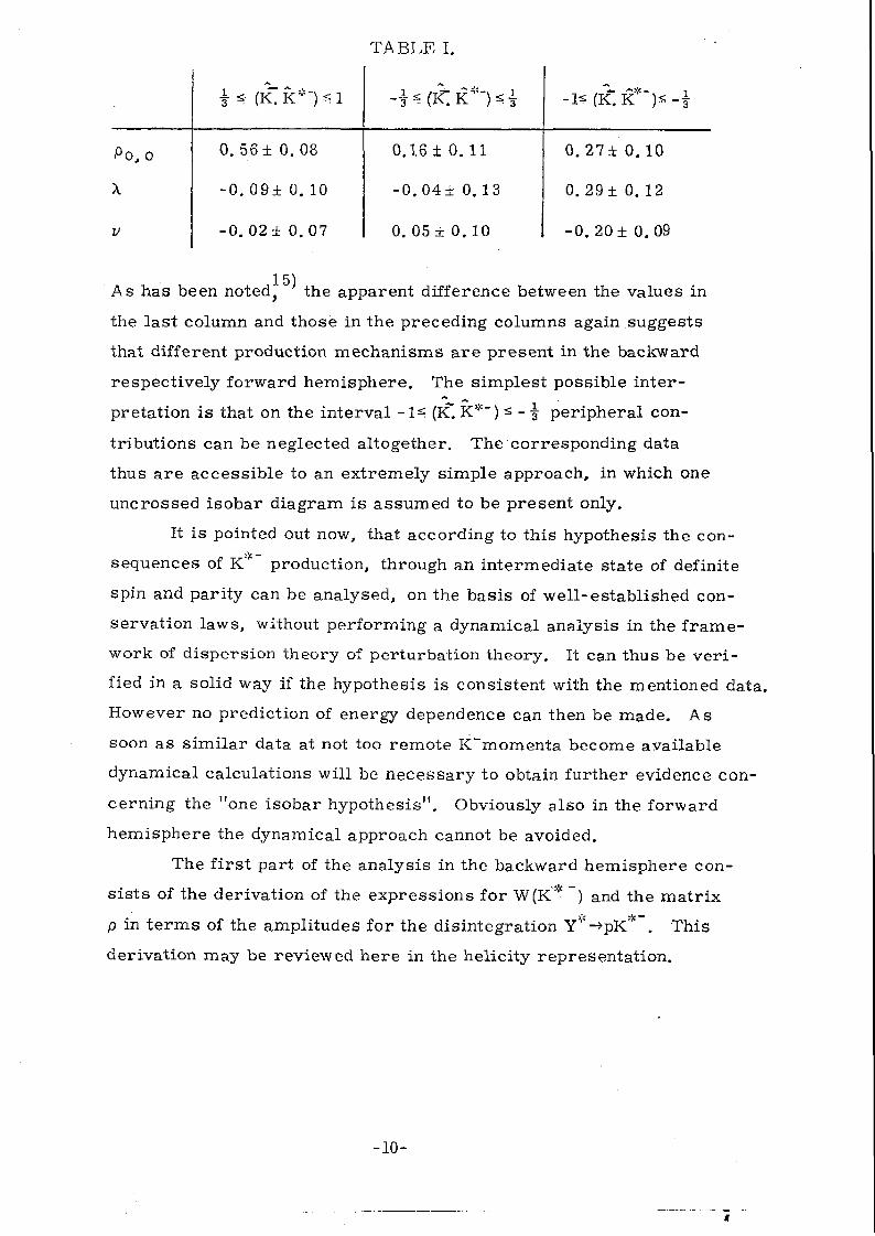
TABLE I.
Po, o
X
V
3
0.
- 0
- 0
* (K.i
56± 0
. 0 9 ±
. 02 ±
.08
0. 10
0.07
i~ 3
0.
- t
0.
SO*
16±
). 04
05 ±
0
±
0
11
0. 13
. 1 0
- 1 -
0.
0.
- 0
27±
29±
. 2 0
0.
0.
± 0
10
12
.09
i~ 3
15)As has been noted^ the apparent difference between the values in
the last column and those in the preceding columns again suggests
that different production mechanisms are present in the backward
respectively forward hemisphere. The simplest possible inter-
pretation is that on the interval -1=» (K, K*~) ^ - i peripheral con-
tributions can be neglected altogether. The corresponding data
thus are accessible to an extremely simple approach, in which one
uncrossed isobar diagram is assumed to be present only.
It is pointed out now, that according to this hypothesis the con-
sequences of K* production, through an intermediate state of definite
spin and parity can be analysed, on the basis of well-established con-
servation laws, without performing a dynamical analysis in the frame-
work of dispersion theory of perturbation theory. It can thus be veri-
fied in a solid way if the hypothesis is consistent with the mentioned data.
However no prediction of energy dependence can then be made. As
soon as similar data at not too remote K'momenta become available
dynamical calculations will be necessary to obtain further evidence con-
cerning the "one isobar hypothesis11. Obviously also in the forward
hemisphere the dynamical approach cannot be avoided.
The first part of the analysis in the backward hemisphere con-
sists of the derivation of the expressions for W(K* ~) and the matrix
p in terms of the amplitudes for the disintegration Yv-*pKv . This
derivation may be reviewed here in the helicity representation.
-10-
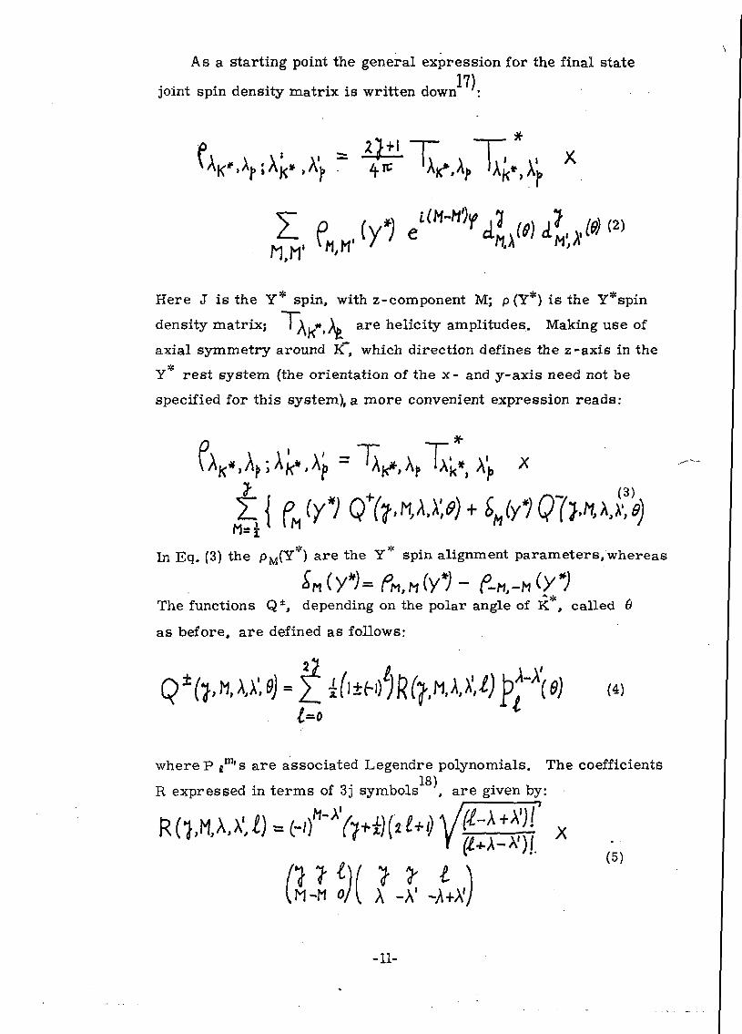
Asa starting point the general expression for the final state
joint spin density m a « x is written down17',
r
Here J is the Y* spin, with z-component M; p(Y*) is the Y*spin
density matrix; 'Ak*.Ai> are helicity amplitudes. Making use of
axial symmetry around K, which direction defines the z-axis in the
Y rest system (the orientation of the x- and y-axis need not be
specified for this system), a more convenient expression reads:
£ { PJY*) Q%t\KK')+SH
In Eq. (3) the PM(Y*) are the Y* spin alignment parameters/whereas
The functions Q*, depending on the polar angle of K , called &
as before, are defined as follows:
fyMU4 bj^(«) (4)
where P (m's are associated Legendre polynomials. The coefficients
R expressed in terms of 3j symbols , are given by:
\fttM y1 ' " (5)
M-M o/{ A -A1 -A+A'J
-11-
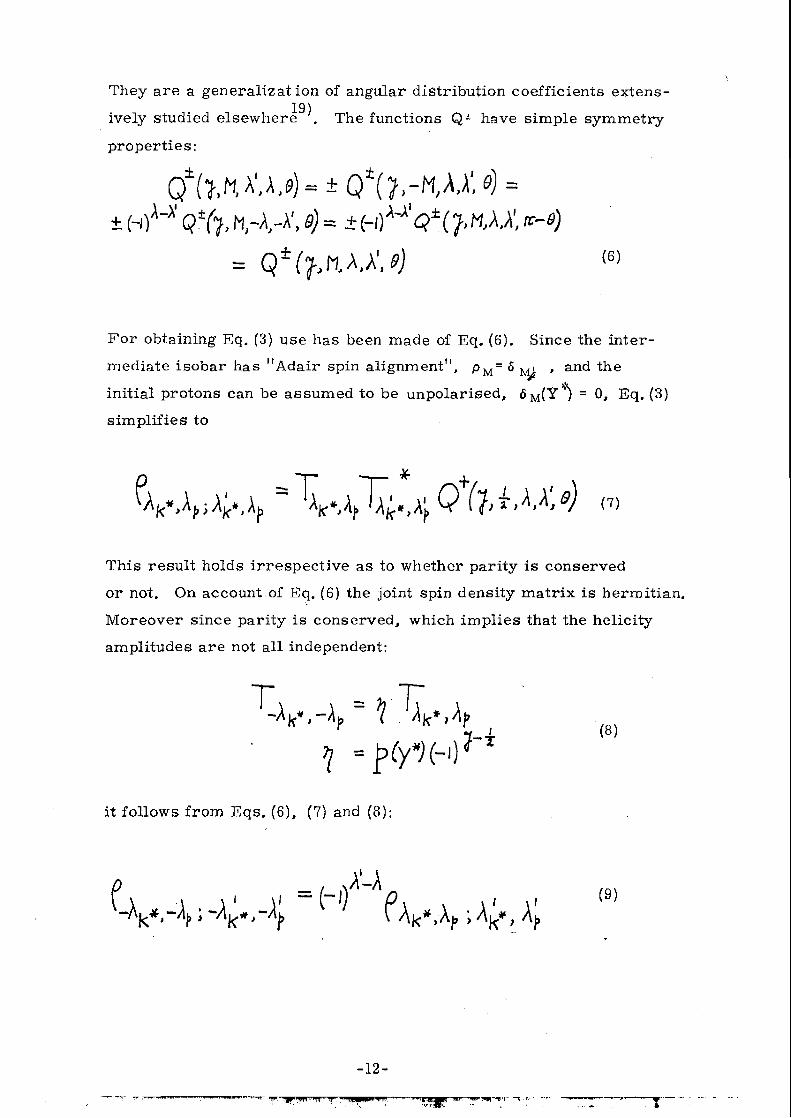
They are a generalization of angular distribution coefficients extens-
ively studie
properties:
19)ively studied elsewhere . The functions Q* have simple symmetry
For obtaining Eq. (3) use has been made of Eq. (6). Since the inter-
mediate isobar has "Adair spin alignment", PM= 5 ^a , and the
initial protons can be assumed to be unpolarised, 6 M(Y ) = 0, Eq. (3)
simplifies to
(7)
This result holds irrespective as to whether parity is conserved
or not. On account of Eq. (6) the joint spin density matrix is hermitian.
Moreover since parity is conserved, which implies that the helicity
amplitudes are not all independent:
it follows from Eqs. (6), (7) and (8):
f 0)
-12-
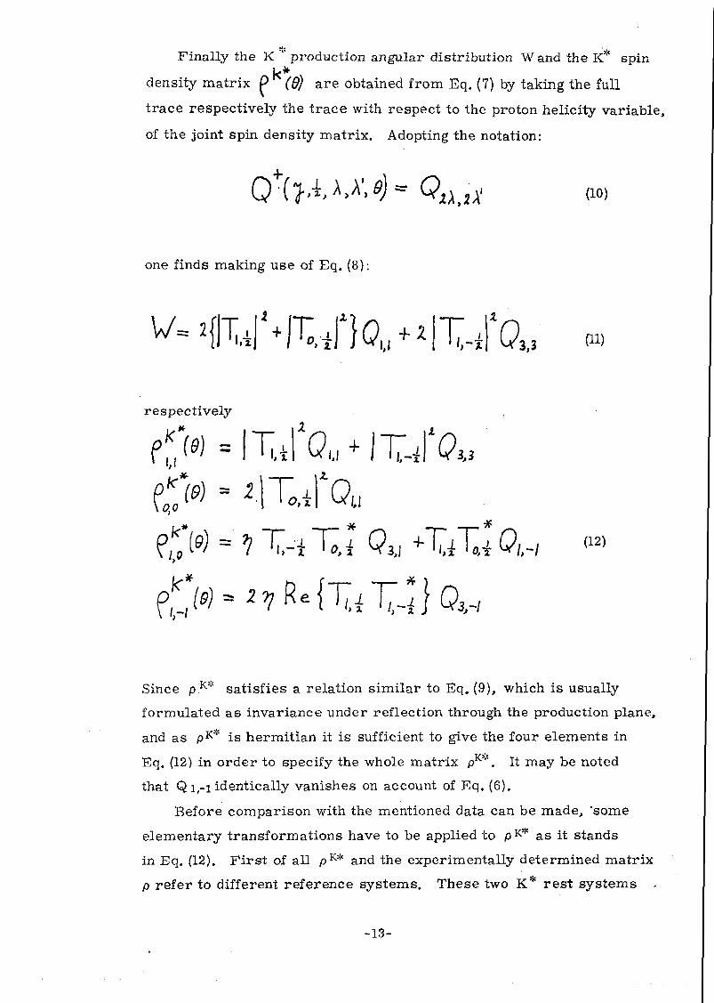
Finally the K production angular distribution W and the K* spin
density matrix P (Q) are obtained from Eq. (7) by taking the full
trace respectively the trace with respect to the proton helicity variable,
of the joint spin density matrix. Adopting the notation:
one finds making use of Eq. (8):
',3 (ii)
respectively
(?,,., (12)
Since pK* satisfies a relation similar to Eq. (9), which is usually
formulated as invariance under reflection through the production plane,
and as pK* is hermitian it is sufficient to give the four elements in
Eq. (12) in order to specify the whole matrix pKv. It may be noted
that Q i,-i identically vanishes on account of Eq. (6).
Before comparison with the mentioned data can be made, 'some
elementary transformations have to be applied to p KV as it stands
in Eq. (12). First of all p K* and the experimentally determined matrix
p refer to different reference systems. These two K* rest systems
-13-
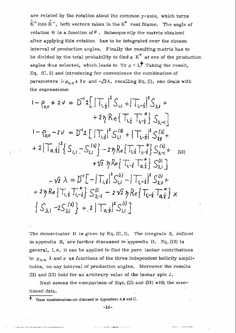
are related by the rotation about the common y-axis, which turns
K*into K", both vectors taken in the K* rest frame. The angle of
rotation 6 is a function of 6 . Subsequently the matrix obtained
after applying this rotation has to be integrated over the chosen
interval of production angles. Finally the resulting matrix has to
be divided by the total probability to find a K at one of the production
angles thus selected, which leads to Tr p = l.T Taking the result,
Eq. (C. 2) and introducing for convenience the combination of
parameters l -p o o±2i / and -,J2A., recalling Eq. (1), one deals with
the expressions:
,-/
:,-/ + (13)
The denominator D is given by Eq. (C. 1). The integrals S, defined
in appendix B, are further discussed in appendix D. Eq. (13) is
general, i. e. it can be applied to find the pure isobar contributions
t° Po.o, *• and v as functions of the three independent helicity ampli-
tudes, on any interval of production angles. Moreover the results
(11) and (13) hold for an arbitrary value of the isobar spin J.
Next comes the comparison of Eqs. (11) and (13) with the men-
tioned data.
' These transformations are discussed in Appendices A,B and C.
-14-
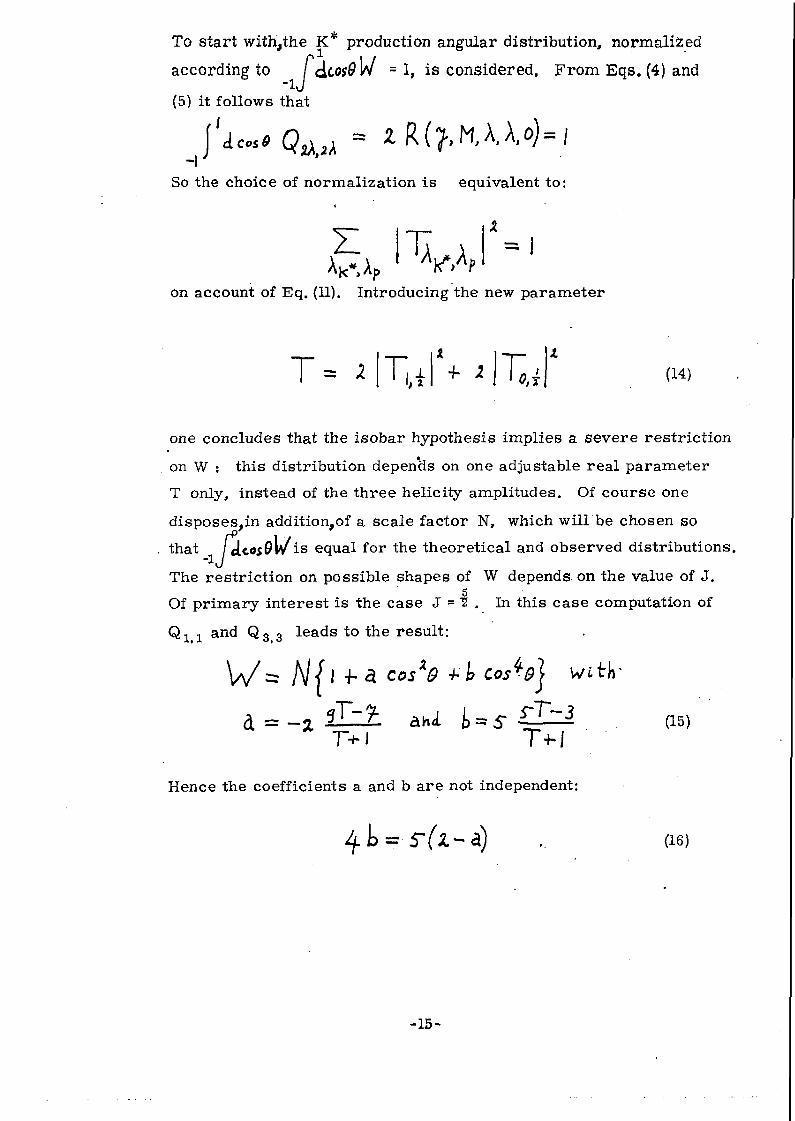
To start withjthe K* production angular distribution, normalized
according to / dcosQw = 1, is considered. From Eqs. (4) and
(5) it follows that
So the choice of normalization is equivalent to:
on account of Eq. (11). Introducing the new parameter
(14)
one concludes that the isobar hypothesis implies a severe restriction
on W : this distribution depends on one adjustable real parameter
T only, instead of the three helicity amplitudes. Of course one
disposes^in addition,of a scale factor N, which will be chosen so
that dtos9v/is equal for the theoretical and observed distributions.
The restriction on possible shapes of W depends on the value of J.5
Of primary interest is the case J = ~2 . In this case computation of1 1 and Q3 3 leads to the result:
i 4"= A/{ COSX9
T+J T+l
Hence the coefficients a and b are not independent:
(16)
-15-
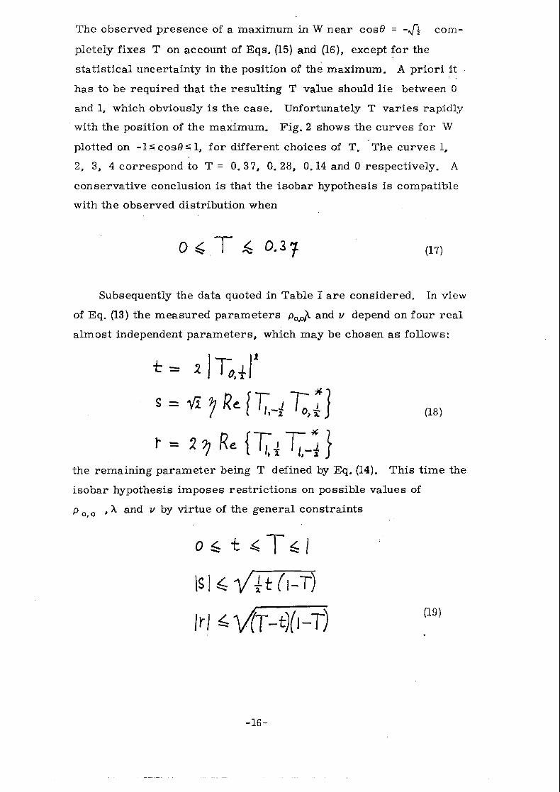
The observed presence of a maximum in W near cos0 = -*f$ com-
pletely fixes T on account of Eqs. (15) and (16), except for the
statistical uncertainty in the position of the maximum. A priori it
has to be required that the resulting T value should lie between 0
and 1, which obviously is the case. Unfortunately T varies rapidly
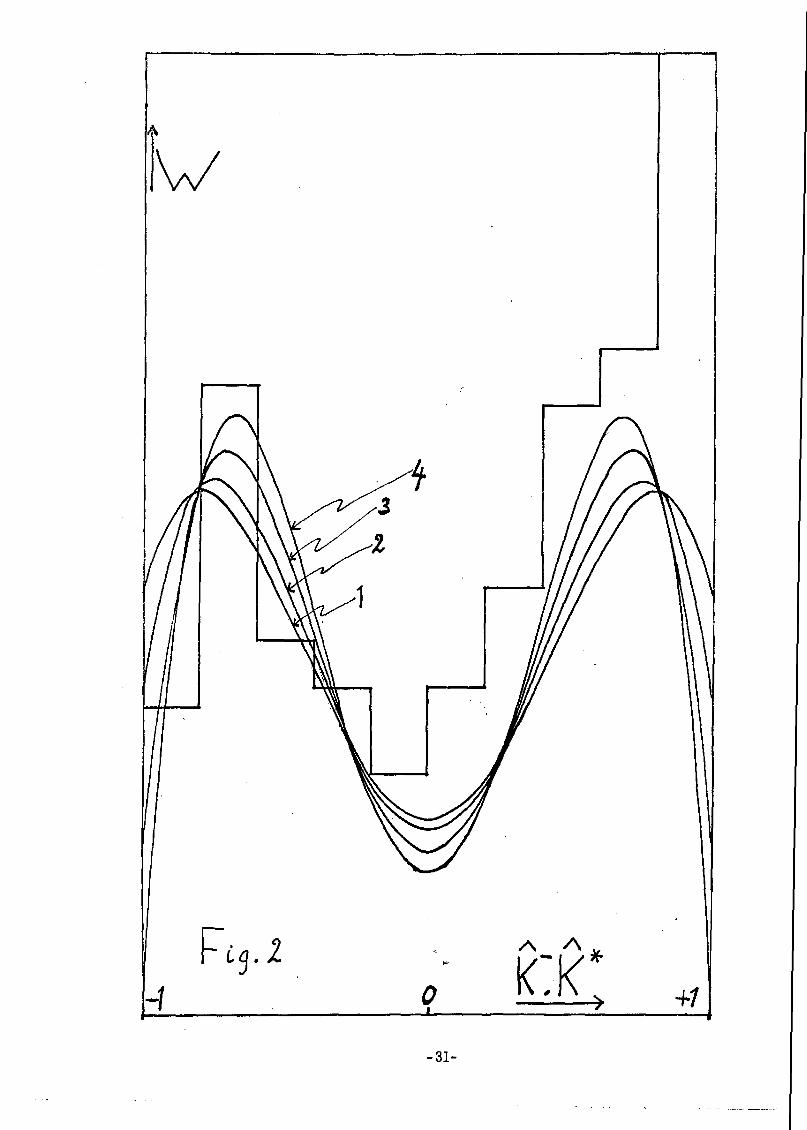
with the position of the maximum, Fig- 2 shows the curves for W
plotted on -l^cosG^l, for different choices of T. The curves 1,
2, 3, 4 correspond to T= 0.37, 0.28, 0.14 and 0 respectively. A
conservative conclusion is that the isobar hypothesis is compatible
with the observed distribution when
o 4T (17)
Subsequently the data quoted in Table I are considered. In view
of Eq. (13) the measured parameters p0>0^. and v depend on four real
almost independent parameters , which may be chosen as follows:
(18)
the remaining parameter being T defined by Eq. (14). This time the
isobar hypothesis imposes restrictions on possible values of
p 0 o , \ and v by virtue of the general constraints
-16-
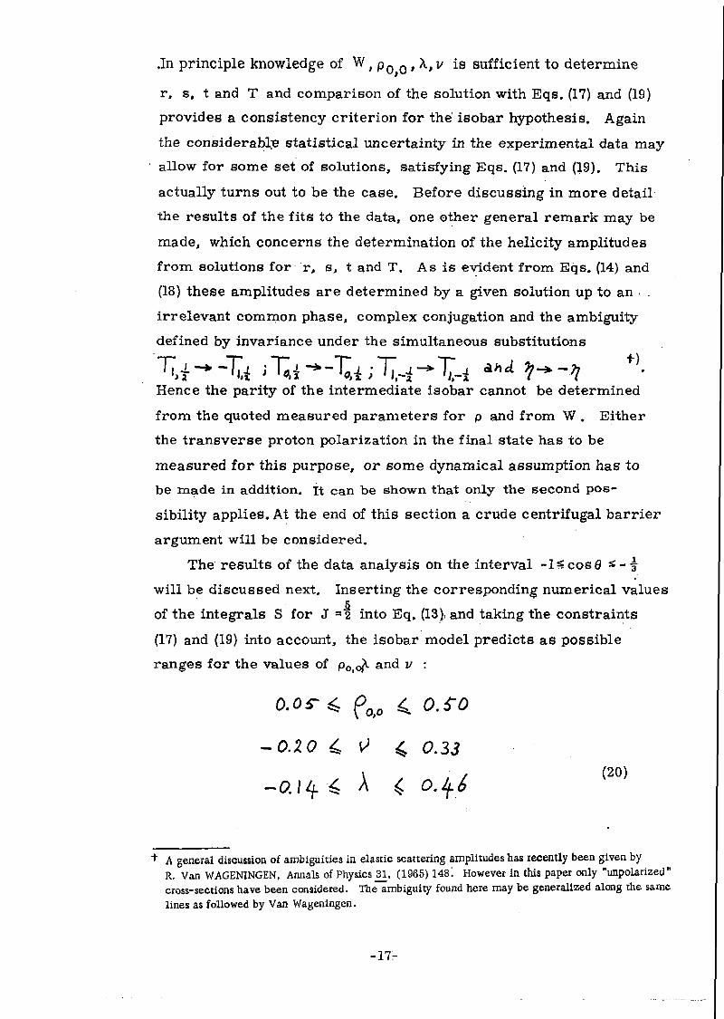
.In principle knowledge of W( pQ Qt x,v is sufficient to determine
r, s, t and T and comparison of the solution with Eqs. (17) and (19)
provides a consistency criterion for the isobar hypothesis. Again
the considerably statistical uncertainty in the experimental data may
allow for some set of solutions, satisfying Eqs. (17) and (19). This
actually turns out to be the case. Before discussing in more detail
the results of the fits to the data, one other general remark may be
made, which concerns the determination of the helicity amplitudes
from solutions for r, s, t and T. As is evident from Eqs. (14) and
(18) these amplitudes are determined by a given solution up to an .
irrelevant common phase, complex conjugation and the ambiguity
defined by invariance under the simultaneous substitutions
Hence the parity of the intermediate isobar cannot be determined
from the quoted measured parameters for p and from W . Either
the transverse proton polarization in the final state has to be
measured for this purpose, or some dynamical assumption has to
be made in addition, it can be shown that only the second pos-
sibility applies. At the end of this section a crude centrifugal barrier
argument will be considered.
The results of the data analysis on the interval -IS cos6 * - |
will be discussed next. Inserting the corresponding numerical values
of the integrals S for J =* 2 into Eq, (13), and taking the constraints
(17) and (19) into account, the isobar model predicts as possible
ranges for the values of pOiO^ and v :
0-05*^ p00 4 oso
-o.zo 4 \> 4 0.3$, \ , * , 1 ( 2 0 )
-0.14- 4 A ^ O.l^b
A general discussion of ambiguities in elastic scattering amplitudes has recently been given byR. Van WAGENINGEN, Annals of Physics 31, (1965) 148! However in this paper only "unpolarized"cross-sections have been considered. The ambiguity found here may be generalized along the samelines as followed by Van Wageningen.
-17-
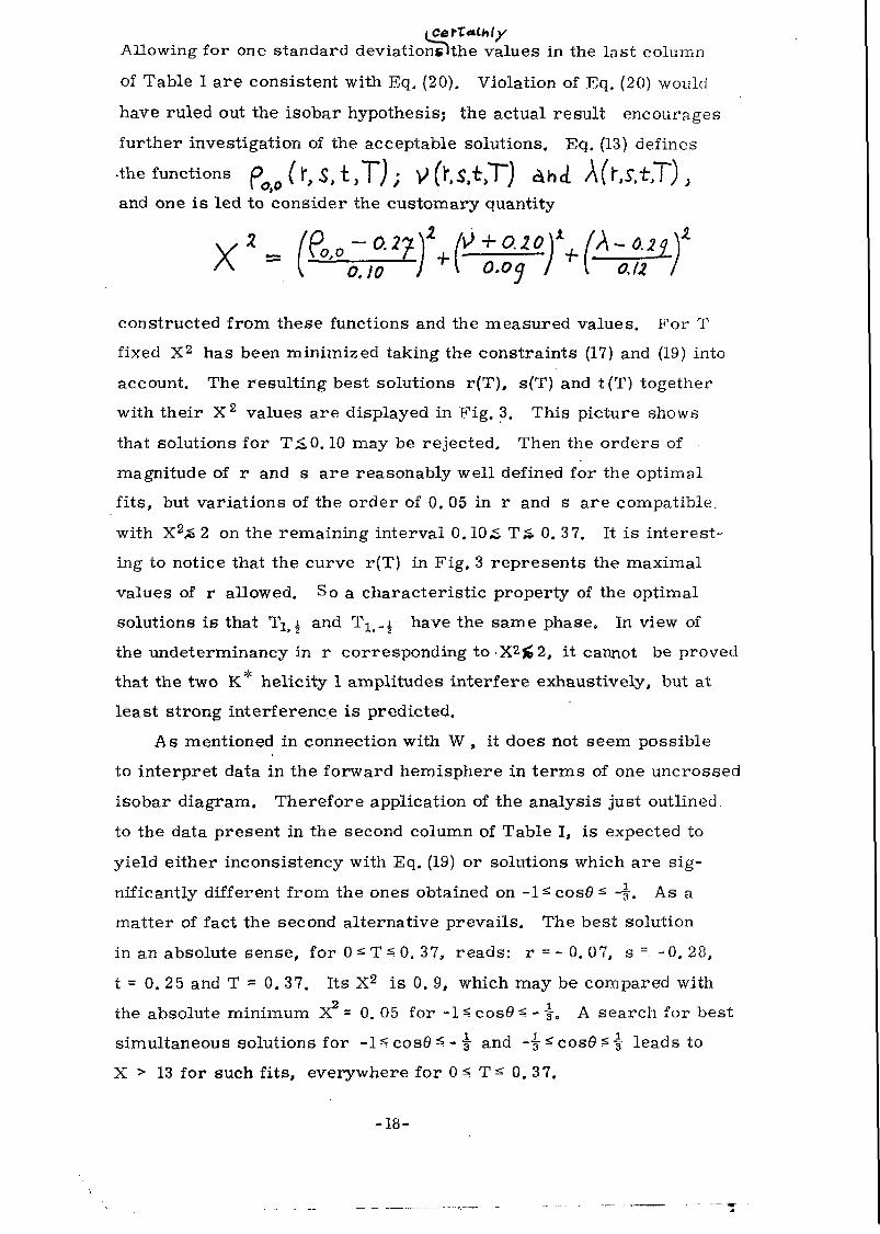
Allowing for one standard deviationsHhe values in the last column
of Table I are consistent with Eq. (20). Violation of Eq. (20) would
have ruled out the isobar hypothesis; the actual result encourages
further investigation of the acceptable solutions. Eq. (13) defines
•the functions f>^( f, S,t >T) ; V> (U*>T) &U X(r,S,±X) }
and one is led to consider the customary quantity
ojd—/ ^ o.o(j I ^1 an
constructed from these functions and the measured values. For T
fixed X2 has been minimized taking the constraints (17) and (19) into
account. The resulting best solutions r(T), s(T) and t(T) together
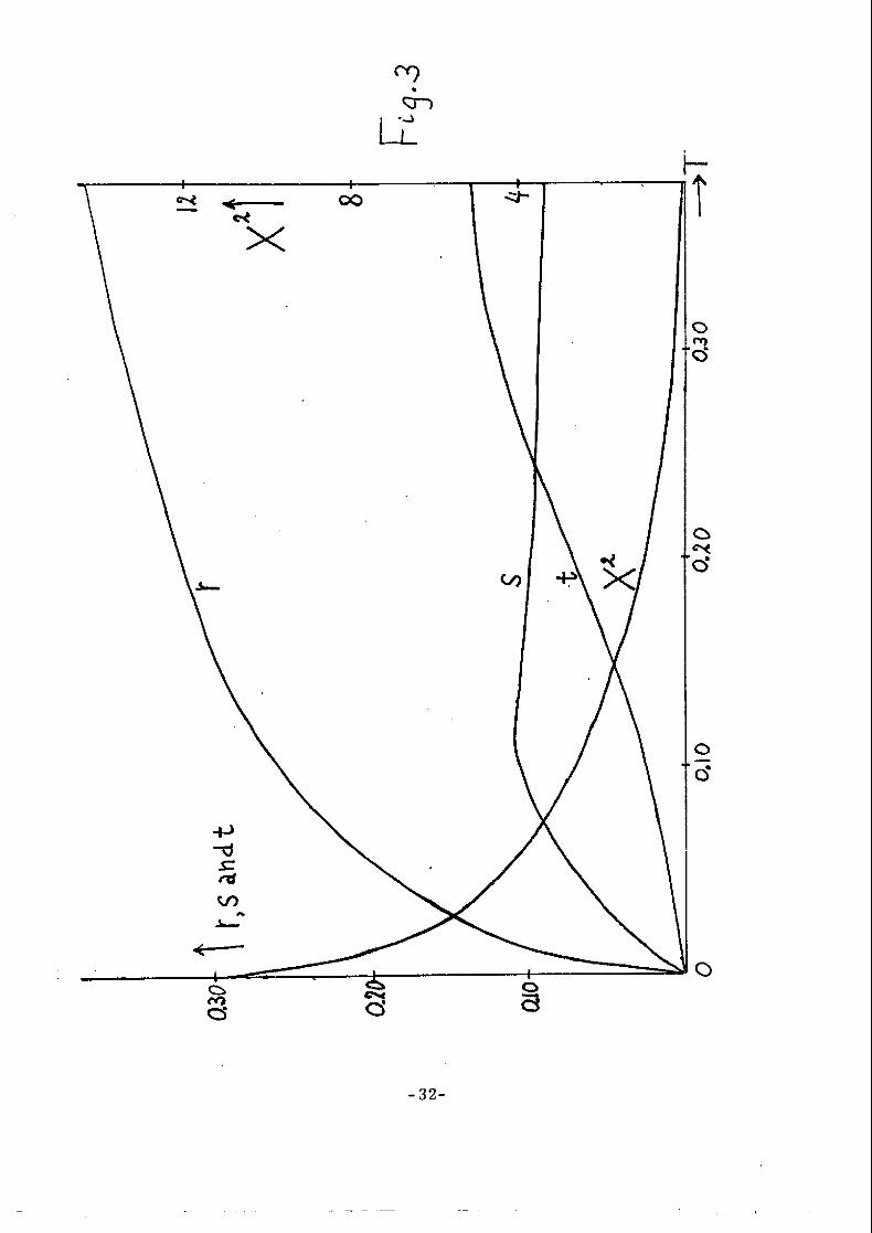
with their X2 values are displayed in Fig. 3. This picture shows
that solutions for T£0.10 may be rejected. Then the orders of
magnitude of r and s are reasonably well defined for the optimal
fits, but variations of the order of 0. 05 in r and s are compatible,
with X2;S 2 on the remaining interval 0.10£ T& 0. 3 7. It is interest-
ing to notice that the curve r(T) in Fig, 3 represents the maximal
values of r allowed. So a characteristic property of the optimal
solutions is that T ^ and T1(.^ have the same phase. In view of
the undeterminancy in r corresponding toX2£2, it cannot be proved
that the two K* helicity 1 amplitudes interfere exhaustively, but at
least strong interference is predicted.
As mentioned in connection with W , it does not seem possible
to interpret data in the forward hemisphere in terms of one uncrossed
isobar diagram. Therefore application of the analysis just outlined
to the data present in the second column of Table I, is expected to
yield either inconsistency with Eq. (19) or solutions which are sig-
nificantly different from the ones obtained on -l^cos0^ - j . As a
matter of fact the second alternative prevails. The best solution
in an absolute sense, for 0 T * 0. 3 7, reads: r = - 0. 0 7, s= -0.28,
t = 0. 25 and T = 0. 37. Its X2 is 0. 9, which may be compared with
the absolute minimum X = 0. 05 for -1 ?? cos(9 - i . A search for best
simultaneous solutions for - l ^ c o s 0 ^ - | and - i =? cos0 ^I leads to
X > 13 for such fits, everywhere for 0 ^ T => 0.37.
-18-
It is concluded that, within the limits of the present non-dynamical
approach, the data at the largest momentum transfers can be sat-
isfactorily interpreted in terms of K* production through a spin |
intermediate isobar. Energetically Yo (1815) is the most plausible
candidate for the isobar. At smaller momentum transfers no such
interpretation is possible, which is attributed to competing peripheral
diagrams. From the fits to the present data, on the interval
- 1£ cos0 £ - i , the helicity amplitudes, describing the disintegration
Y""-»pK*, might be determined approximately and up to some ambig-
uities in phases. Higher precision in the data is needed, for an accurate
determination of the helicity amplitudes, which in turn will provide
valuable information concerning the Y*NK* coupling. Moreover
knowledge of these amplitudes will facilitate the analysis of the data
at smaller momentum transfers, in the framework of an "isobar-
peripheral" model. Here some common features of the acceptable
solutions for the helicity amplitudes may be mentioned, without
going into details. Fig. 3 contains almost all the necessary information
for obtaining details.
For X2S2 T1(.i is the largest amplitude and TOfi and T1($
are of the same order of magnitude. The relative phase of Tlf_±
and T .1 is zero or finite and small for P (Y*) = +, which is sufficient
to characterize also the solutions for opposite parity. The relative
phase of T0 ( | and T1§.i is of the order of 60°± 30°
The corresponding JLS amplitudes; p3, f3 and fi forP(Y^) = +,17)
and ds, g3, d-^ for opposite parity, are readily obtained . Being
mainly interested in their magnitudes, it is sufficient to mention
that |p3 ] >|f3 [ y |f]J respectively [ d3] >| g3[«rj d j . Some solutions
exist for which \ f3j« [ f j respectively [ g3|<( | dj[ . At each
inequality maximal differences in magnitude are of the order of a
factor 2. 5.
Evidently none of the solutions for P(Y") = ± is in clear con-
tradiction with what might be expected on the basis of the centri-
fugal barrier effect. However it is pointed out that in particular
for the optimal solutions one has j g3\<z \ d j , whereas always
[p3 \y J f3[ . This is a weak indication in favour of P(YV) =+, support-
ing the hypothesis Y = YO'(1815).
-19-
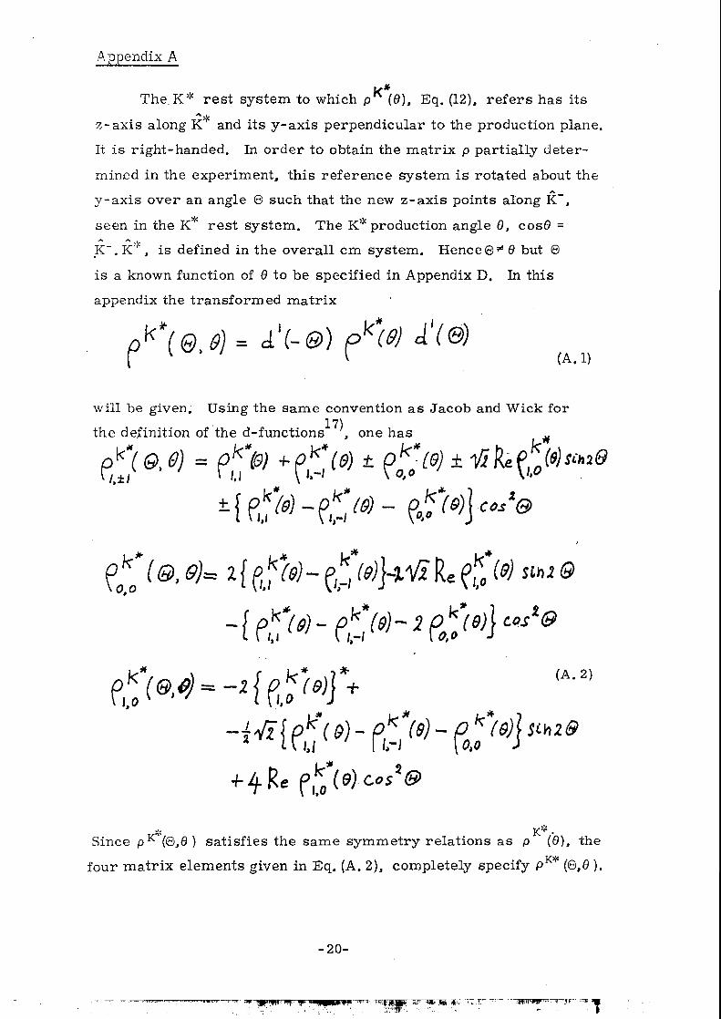
Appendix A
k*
The.K* rest system to which p (9), Eq. (12), refers has its
z-axis along K and its y-axis perpendicular to the production plane.
It is right-handed. In order to obtain the matrix p partially deter-
mined in the experiment, this reference system is rotated about the
y-axis over an angle 6 such that the new z-axis points along K~,
seen in the K* rest system. The K* production angle 6, cosB =
K~.KV, is defined in the overall cm system. Hence©* 8 but 6
is a known function of 0 to be specified in Appendix D. In this
appendix the transformed matrix
Q 9] = d'(-(#' V (A.I)
will be given. Using the same convention as Jacob and Wick for
+
17)the definition of the d-functions , one has
, &)= 1 { tf(9) $')}*& Re tf SttI
,*)=-Zip*(9)] +(A. 2)
'°-iV7l£>k%)- Pk (9)- Ok
0,0
Since pK (8,6) satisfies the same symmetry relations as p (6), the
four matrix elements given in Eq. (A. 2), completely specify PK* (€>,8 ) .
- 2 0 -
' P»f sJS .((i.-
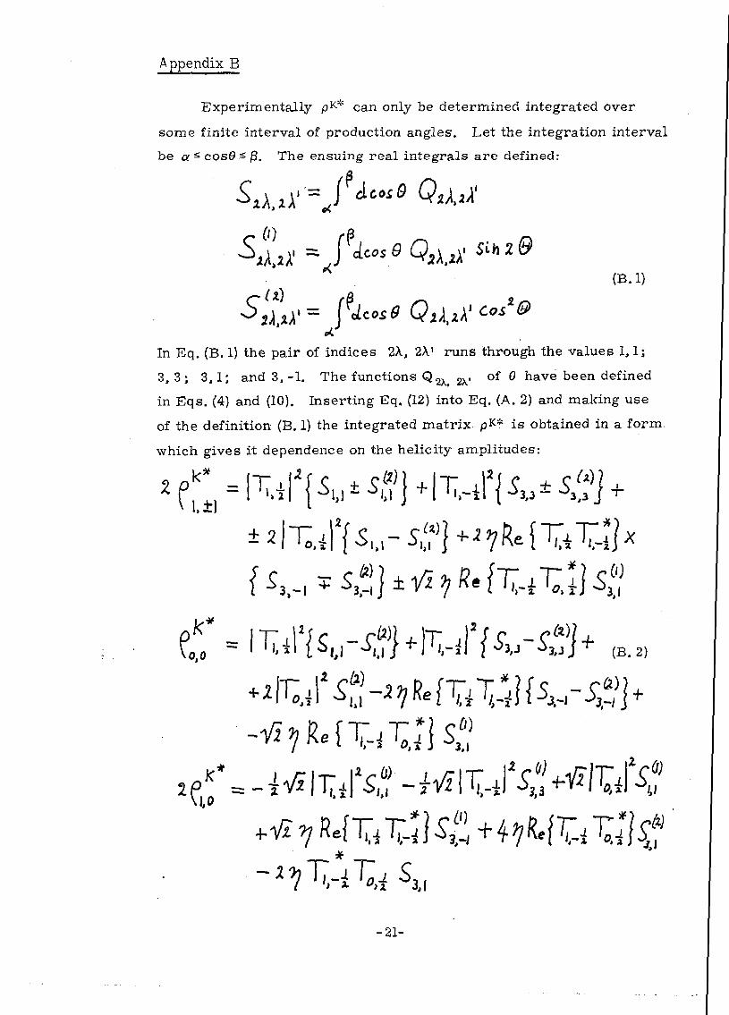
Appendix B
Experimentally pK* can only be determined integrated over
some finite interval of production angles. Let the integration interval
be a £ cos0 S |3. The ensuing real integrals are defined:
(B.l)
In Eq. (B. 1) the pair of indices 2X, 2X1 runs through the values 1,1;
3,3; 3,1; and 3,-1. The functions Q2Xf ^ of 6 have been defined
in Eqs. (4) and (10). Inserting Eq. (12) into Eq. (A. 2) and making use
of the definition (B, 1) the integrated matrix pK* is obtained in a form,
which gives it dependence on the helicity amplitudes:
-21-
Again Eq. (B. 2) completely specifies pK*. The contributing products
of helicity amplitudes are weighted by suitable combinations of
integrals S. These integrals are discussed in Appendix D.
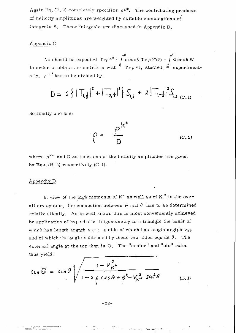
Appendix C
r3 rfl
As should be expected TrpK¥= / dcos 0 Tr pK*(6) = / dCos0W
In order to obtain the matrix p with a Trp = lJ studied a experiment-•tr
ally, p has to be divided by:
So finally one has:
_ p(C 2,
where pK* and D as functions of the helicity amplitudes a re given
by Eqs. (B. 2) respectively (C.I).
Appendix D
In view of the high momenta of K~ as well as of K in the over-
all cm system, the connection between 0 and 6 has to be determined
relativistically. As is well known this is most conveniently achieved
by application of hyperbolic trigonometry in a triangle the basis of
which has length argtgh vK- • a side of which has length argtgh vK*
and of which the angle subtended by these two sides equals 9. The
external angle at the top then is 6. The "cosine" and "sin" rules
thus yield:
SLh ti> =Z B cos9
- 2 2 -
• i • * • . - • . . •
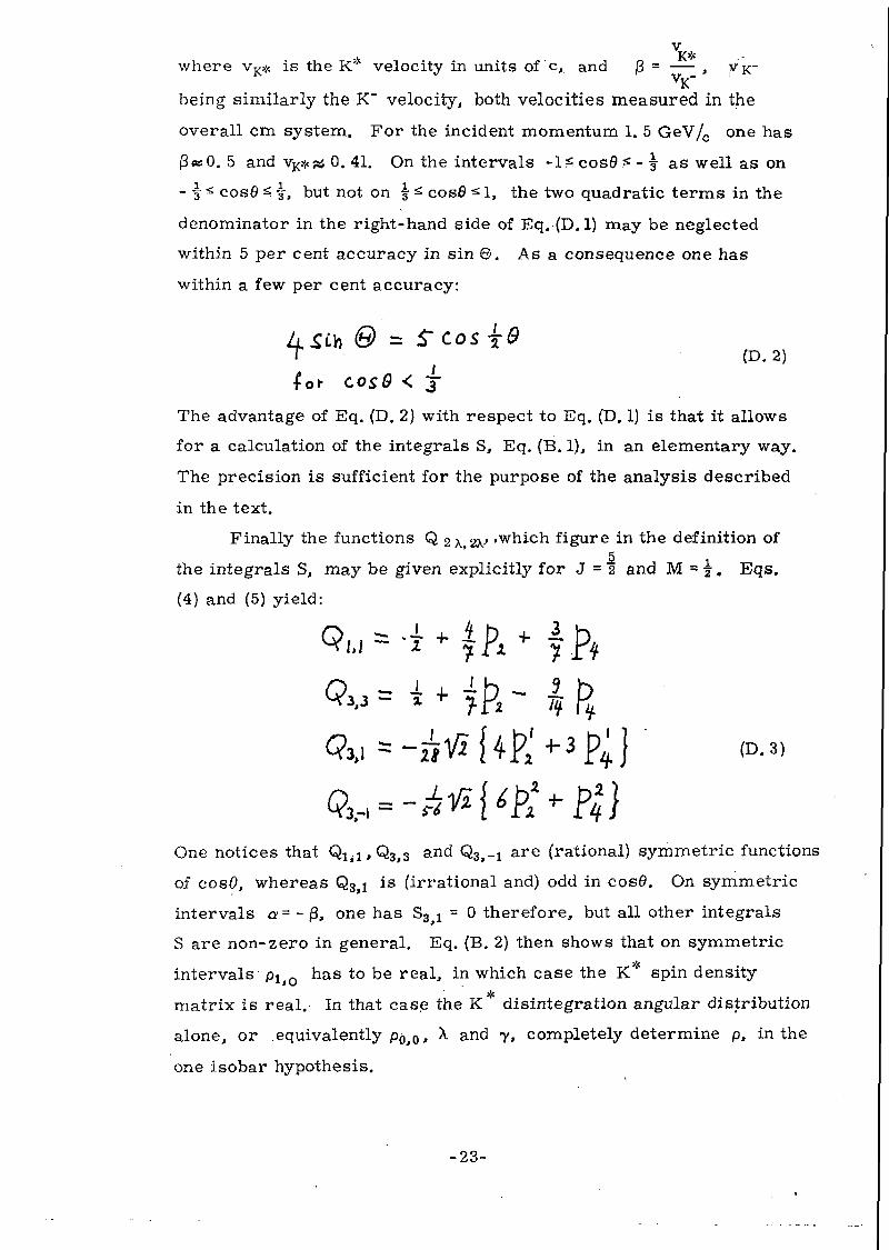
VK*where vK# is the K* velocity in units of c, and fi = -111 ,
vK-
being similarly the K" velocity, both velocities measured in the
overall cm system. For the incident momentum 1. 5 GeV/c one has
|3«0. 5 and vK*s* 0. 41. On the intervals - l^cos f l^ - j as well as on
- \ s cos© i , but not on ^ ^ cosS * 1, the two quadratic terms in the
denominator in the right-hand side of Eq. (D.1) may be neglected
within 5 per cent accuracy in sin 8 . As a consequence one has
within a few per cent accuracy:
for cosQ < X
The advantage of Eq. (D. 2) with respect to Eq. (D. 1) is that it allows
for a calculation of the integrals S, Eq. (B. 1), in an elementary way.
The precision is sufficient for the purpose of the analysis described
in the text.
Finally the functions Q 2 \# 2X> -which figure in the definition of5
the integrals S, may be given explicitly for J = 2 and M = -|. Eqs.
(4) and (5) yield:
One notices that Q l iX, Q3j3 and Q3>-! are (rational) symmetric functions
of cos#, whereas Q3jl is (irrational and) odd in cos0. On symmetric
intervals a = - |3, one has S3 x = 0 therefore, but all other integrals
S are non-zero in general. Eq. {B. 2) then shows that on symmetric
intervals p l j 0 has to be real, in which case the K* spin density
matrix is real. In that case the K disintegration angular distribution
alone, or .equivalently pOjO, X and y, completely determine p, in the
one isobar hypothesis.
- 23 -
ACKNOWLEDGEMENTS
The author is indebted to the International Atomic Energy
A gency, and in particular to the director of the International
Centre for Theoretical Physics, Professor Abdus Salam, for a
profitable stay at ICTP, Trieste. This work partially belongs
to the research programme of the "Stichting voor Fundamenteel
Onderzoek der Materie" F.O.M., financially supported by the
"Nederlandse Organisatie voor Zuiver Wetenschappelijk Onder-
zoek", Z.W.O. He wishes to thank Professors J. Kluyver and
Su Wouthuysen for their continuous interest in this work. He
gratefully acknowledges some discussions on the subject with
Professors A.O. Barut, S. Berman, K. Nishijima and J. Werle
at ICTP.
-24 -
REFERENCES
1) A recent account of the peripheral model applied to inelastic
resonance production is : The Peripheral Model with Form
Factors , G. C. FOX. Preprint Department of Applied
Mathematics and Theoretical Physics, University of Cambridge,
Cambridge, England, February 1965.
One pion exchange in the processes KN->NK* has been cal-
culated in detail e . g . by V. BERZI, E. RECAMI,
Preprint Instituto di Fisica dell1 University, Milano, IFUM -
010/Sp, March 1965.
2} K. GOTTFRIED, J. JACKSON, Nuovo Cimento 33,(1964) 309.
J. JACKSON, H. PILKUHN, Nuovo Cimento 3£, (1964) 906,
with erratum in Vol.^4 (1964) 1841.
J. JACKSON, Nuovo Cimento £4 (1964) 1644.
M. FERRO-LUZZI, R. GEORGE, Y. GOLDSCHMIDT-CLERMONT,
V. HENRI, B. JO NGEJAMS, D. LEITH, G. LYNCH, F .
MULLER, J. PERREAU, Preprint CERN/TC/Physics 65-6,
February 1965. To be published in Nuovo Cimento.
3) Ph. SALIN, Nuovo Cimento ^8 (1963) 1384.
C. HOHLER, W. SCHMIDT, Annals of Physics, 28 (1964) 34.
4) G. SMITH, J. SCHWARTZ, D. MILLER, G. KALBFLEISCH,
R. HUFF, O. DAHL, G. ALEXANDER, Phys. Rev. Letters
_10 (1963) 138,
G. CHADWICK, D. CRENNELL, W. DA VIES, H. DERRICK,
J. MULVEY, P. JONES, D. RADOJICIC, C. WILKINSON,
A. BETTINI, H. CRESTI, S. LAMENTANI, L. PERRUZZQ,
R. SANTANGELO, Physics Letters 6 (1963) 309.
H. FERRO-LUZZI, R.GEORGE, Y. GOLDSCHMIDT-CLERMONT,
V. HENRI, B. JONGEJANS, D. LEITH, G. LYNCH, F . MuLLER,
J. PERREAU, Proc. of the Sienna International Conf.
on Elementary Part icles, Vol. I (1963)188.
-25 -
5) K. GOTTFRIED, J. JACKSON, Nuovo Cimento ^4 (1964) 735,
with erratum in Vol.^4 (1964) 1843.
M. FERRO-LUZZI et a l . , viz. Ref. 2.
6) K. DIETZ, H. PILKUHN, Preprint CERN 10013/TH. 450,
December 1964.
7) W. COOPER, H. FILTHUTH, A. FRIDMAN, E. IVtALAMUD,
H, SCHNEIDER, E. GELSEMA, J. KLUYVER, A. TENNER,
Proc. of the Sienna Int. Conf. on Elementary Part icles, Vol.
I (1963) 160.
8) R. ADAIR, Preprint CERN/TH/63-12, July 1963/Back-
ground Amplitudes and the spin of the Yj* .
9) A similar suggestion has been made by E. MALAMUD, P.
SCHLEIN, Physics Letters _1£ (1964) 145.
10) Diagrams assumed to contribute to the reaction ;r+p-» E+K+
are the ones for one K* exchange; intermediate isobars
Ng;< (1238) and N3* (1920); respectively an uncrossed iso-t 2
bar diagram with a A hyperon in the intermediate state.
This model yields satisfactory fits to differential cross-section
and L+ polarization from threshold to 1. 8 GeV/c incident
momentum (Lab). L. EVANS, J. KNIGHT, Phys. Rev.137 (1965) B1232. A simpler case is the reaction "jr'+N->i:K* + asstudied by C.H. CHAN, Y. LIU, Nuovo Cim.^5 (1965) 298.
11) Compare e.g. M. ROOS, Nuclear Physics, J52 (1964) 1, or
A. G. TENNER, G. F . WOLTERS, Progress of Elementary
Particle and Cosmic Ray Physics, to be published.
-26 -
12) J. BADIER, H. DEMOULIN, J. GOLDBERG, B.GREGORY,
P. KREJBICH, C. PELLETIER, H. VILLE, R. BARLOUTAUD,
A. LEVEQUE, C. LOUEDEC, J. MEYER, P. SCHLEIN,
E. GELSEMA, W. HOOGLAND, J. KLUYVER, A. TENNER,
Proc. of the 1964 Dubna Int. Conf. on High Energy Physics,
to be published.
13) G. CHADWICK et a l . , viz. Ref.4.
14) M. FERRO-LUZZI et al. , viz Refs. 2 and 4.
15) E. GELSEMA, J. KLUYVER, A. TENNER, G. WOLTERS
Physics Letters H) (1964) 341.
16) A detailed description of the experiment in question is given
by E. GELSEMA, doctoral thesis, University of Amsterdam,
Amsterdam, to be published.
17) M. JACOB, G. C. WICK, Annals of Physics 1_ (1959) 404.
Description of disintegrations in helicity representation has
earl ier been given by M. JACOB, Nuovo Cimento 9 (1958) 826.
18) Numerical values have been taken from: M. ROTENBERG,
R. BIVINS, N. METROPOLIS, J. WOOTEN J r . , the 3-j and
6-j symbols, the Technology P re s s , MIT, Cambridge,
Massachusetts, 1959.
19) G. WOLTERS, Proc. Kon. Ned. Acad. Wetenschappen, Series
B, 67 (1964) 192.
- 2 7 -
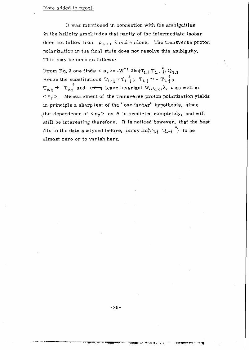
Note added in proof:
It was mentioned in connection with the ambiguities
in the helicity amplitudes that parity of the intermediate isobar
does not follow from pOiO , X and y alone. The transverse proton
polarization in the final state does not resolve this ambiguity.
This may be seen as follows:
From Eq. 2 one finds. < sy>= -W"1 2frn{T1) i TXi_ |} Q l 3
Hence the substitutions Tlt_|-> T ^ ; Tlp i -» - Tlt\ j
T o j -*- T o | and rr***r\ leave invariant W#p001A, v as well as
< Sy >, Measurement of the transverse proton polarization yields
in principle a sharp test of the "one isobar" hypothesis, since
vthe dependence of <Sy> on 6 is predicted completely, and will
still be interesting therefore. It is noticed however, that the best
fits to the data analysed before, imply ImfTi^ Ti(-£ } to be
almost zero or to vanish here.
- 28 -
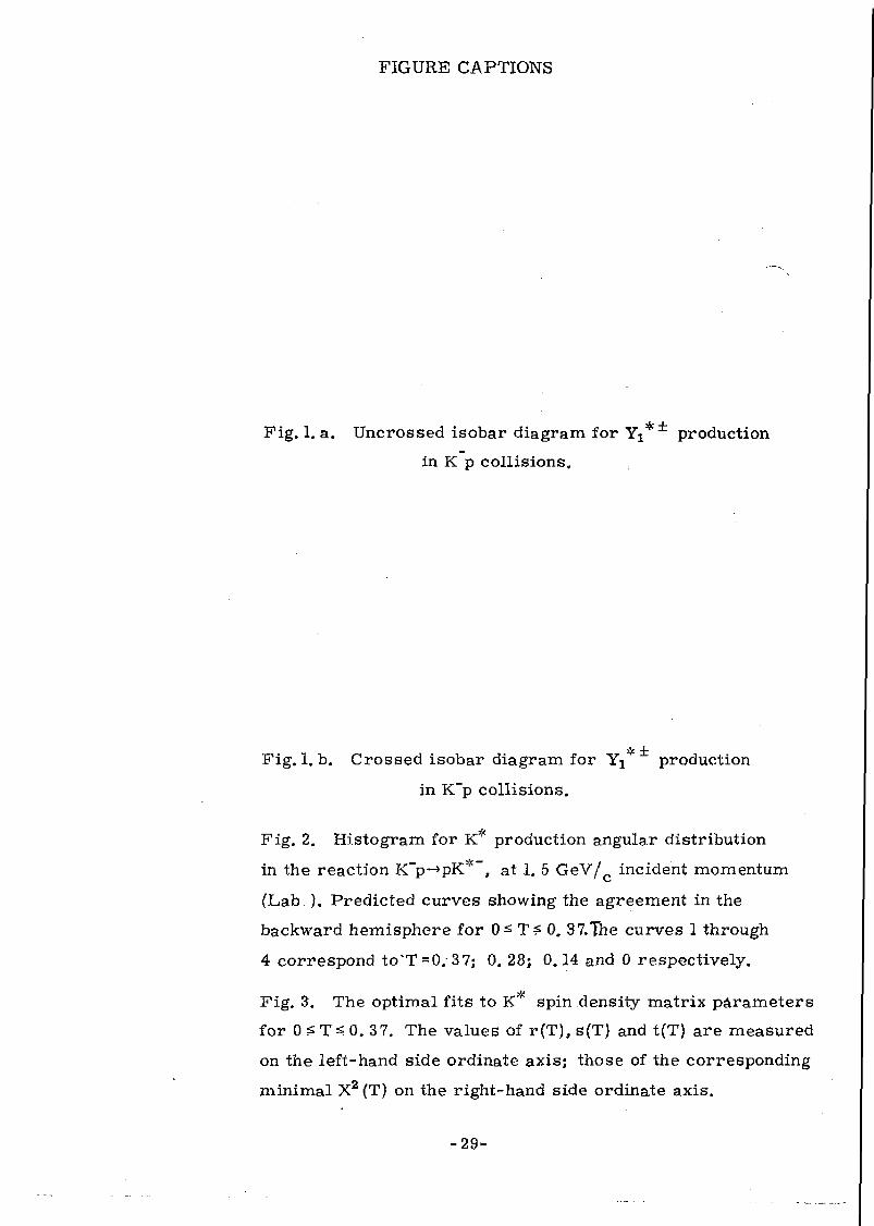
FIGURE CAPTIONS
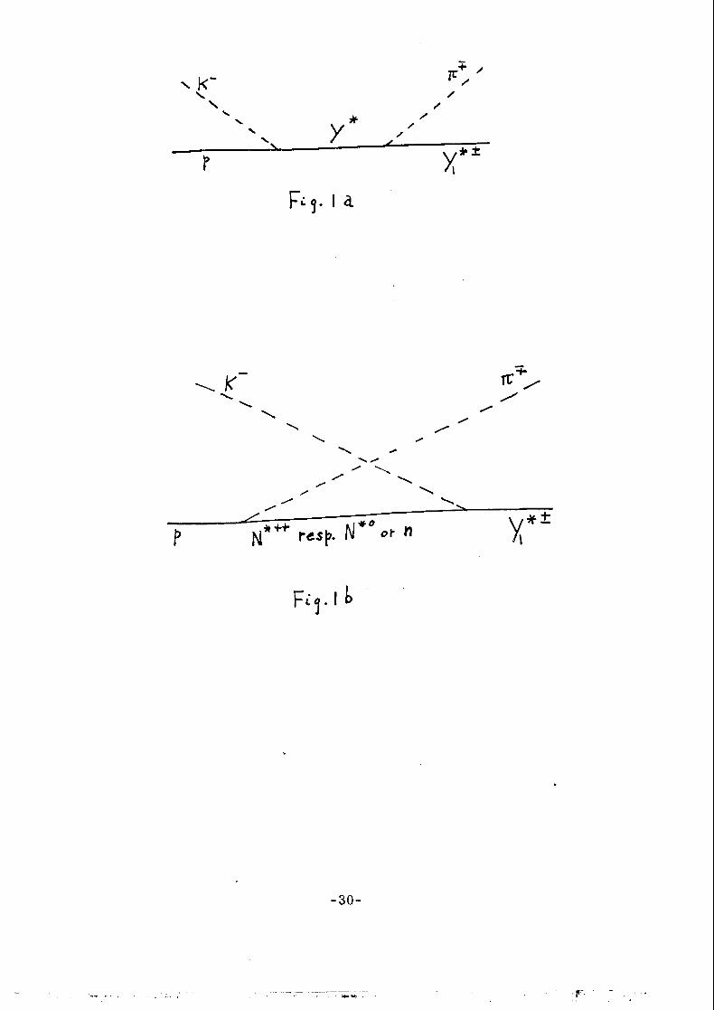
Pig. 1. a. Uncrossed isobar diagram for Yj** production
in K p collisions.
Fig. 1. b. Crossed isobar diagram for Yj production
in K~p collisions.
Fig. 2. Histogram for K* production angular distribution
in the reaction K~p-*pK*~, at 1. 5 GeV/c incident momentum
(Lab ). Predicted curves showing the agreement in the
backward hemisphere for 0^ T? 0. 37.The curves 1 through
4 correspond to*T=0.37; 0. 28; 0.14 and 0 respectively.
Fig. 3. The optimal fits to K* spin density matrix parameters
for 0 T^ 0. 3 7. The values of r(T), s(T) and t(T) are measured
on the left-hand side ordinate axis; those of the corresponding
minimal X2 (T) on the right-hand side ordinate axis.
- 2 9 -
y y
j . i a
X
F i j . l t
- 3 0 -
-31-
- 3 2 -