IS­ENES WP4OASIS Dedicated User Support 2010

Annual reportE. Maisonnave, S. Valcke

TR/CMGC/11/28

Abstract

Three missions complemented the OASIS Dedicated User support program in 2010. Focused on high performance configurations, these actions consisted in:

• testing OASIS3 on a high resolution global model: EC-Earth, IFS-NEMO (SMHI, Norrköping)

• implementing 2 new OASIS4 coupling interfaces in regional coupled models : COSMO-CLM (ETHZ, Zürich) and WRF-NEMO (LOCEAN-CNRS, Paris)

The first mission helped to have a better idea on OASIS3 limitations for high resolution models on scalar machine: The OASIS3 mono-process cost (~6 s per coupling step) is not negligible compared to Ec-earth3 T799-ORCA025 coupling step duration (e.g. 33.2 sec in the 800-256-1 configuration) leading to a coupling overhead of 11% on an Opteron-Infiniband cluster. But an optimal use of parallel version of OASIS3 on 10 processes could reduce this overhead down to 1.3%. Limits of OASIS3 are not yet hit but could be reached on this machine, if IFS model continues to scale for more than 3000 cores (as described by ECMWF), or on MPP architectures (CRAY XT, IBM BG) with equivalent number of resources, or on any other machine if the component models can be distributed so to reach a quasi perfect load-balancing.

This emphasises that the need for an efficient coupling on massively parallelized configurations is becoming a reality for high-end configurations.

Switching from a per-subroutine-call coupling to OASIS4, the COSMO-CLM coupled model is now a modular system, where components can have different time stepping and different spatial discretizations. Many limitations remain however. First, only the master process of CLM gathering the whole coupling fields is for now communicating with OASIS4 because CLM partitioning is not currently supported by OASIS4. Second, a strong slowing down is observed in OASIS4 exchanges when the number of CLM processes increases, even though they are not involved in the coupling.

With WRF-NEMO model, the existing OASIS3 model interfaces have been successfully upgraded to OASIS4. Nevertheless, too many issues remains to attribute a scientific validity to the coupling such as problem in the reading of the coupling restart files and issue with completely masked partitions. Furthermore, even if OASIS4 computational cost appears significantly low (less than 1% of the total WRF-NEMO calculation duration), failures on parallel interpolation weight calculation forbid to fully validate coupler scalability when the number of cores is increased, e.g. for more than 128 cores when the nearest neighbour interpolation is used and even for a lower number of cores with other interpolations.

Due to the observed defects, we strongly suggest to limit OASIS4 support to a few limited number of already implemented configurations, in order to solve the observed problems before envisaging other coupled systems.

Thanks to Uwe Fladrich, Klaus Wyser, Colin Jones (SMHI), Chandan Basu, Torgny Faxén (NSC), Edouard Davin, Sonia Seneviradne, Anne Roches (ETHZ), Olivier Fuhrer (MeteoSwiss), Jean-Guillaume Piccinalli (CSCS), Sébastien Masson, Guillaume Samson, Claire Lévy (LOCEAN) for their strong support and the constant interest for our work. Once again, thanks to our four OASIS developers, Moritz Hanke, Rene Redler (DKRZ), Sophie Valcke and Laure Coquart (CERFACS).

Estimated carbon emission diagnostic for those 3 journeys by terrestrial means of transport: 230Kg

Mission #4Oct 18­ Nov 12 2010

Host: Uwe FladrichLaboratory: SMHI, Norrköping (Sweden)

Main goal: Test performances of the OASIS3 based Ec­earth high resolution model

Main conclusion

The OASIS3 mono­process cost  (~6 s per coupling step)  is not negligible compared to Ec­earth3   T799­ORCA025   coupling   step   duration  (e.g.   33.2   sec   in   the   800­256­1 configuration)  leading to a coupling overhead of 11% on an Opteron­Infiniband cluster. But an optimal use of  parallel  version of  OASIS3 on 10 processes  could reduce this overhead down to 1.3%. Limits of OASIS3 are not yet hit but could be reached on this machine,  if  IFS model continues to scale for more than 3000 cores (as described by ECMWF),  or   on   MPP   architectures   (CRAY   XT,   IBM   BG)   with   equivalent   number   of resources, or on any other machine if the component models can be distributed so to reach a quasi perfect load­balancing. 

Model / machine description

SMHI’s coupled model (high resolution version) deals with:

− IFS, cycle 36: T799, 843.490 grid points, ˜25Km, 62 vertical levels, time step: 720s− NEMO, v3.2: ORCA025, 1.472.282 grid points, ˜40Km, 45 vertical levels, time step: 

1200s− OASIS v3 (pseudo parallel)

20 coupling fields are exchanged between the two components at a coupling frequency of 3 hours. The model is available on Ekman supercomputer, 1.268 compute nodes of 2 quadripro   AMD   Opteron   (#   10.144),   Infiniband   interconnection,   located   at   Royal Institute of Technology (KTH), Stockholm, center for parallel computers (PDC). 

Evaluation of Oasis additional cost

At such high resolution,  on a scalar  machine,   the  limited parallelism of  OASIS could become a bottleneck for the coupled simulation. We propose to determine the OASIS cost   (communications   and   interpolation   calculations)   and   its   impact   on   the   global performances of the model.

The best load balancing between ocean and atmosphere models has to be reached first. At this point,  the coupling overhead can be   measured as the difference between the elapse time of the slowest stand alone model and the elapse time of the whole coupled 

system1.

The resource ratio found for NEMO/IFS load balancing is about  ¼  if  IFS runs on 512 cores (i.e. NEMO should then run on  128 cores). Increasing the number of cores, NEMO seems less scalable than IFS, and ideal ratio reaches 1/3, i.e. NEMO should run on 256 cores when IFS runs on 800 cores. 

Note that a  a limit of 1546 cores (1280­256­10) was  reached (results are not shown). This limitation is probably due to machine implementation of scaliMPI (SMHI and NSC are currently working on an OpenMPI version).

On the following table, all figures represent the elapse time for one coupling time step, mean of the 15 first coupling time steps (45 hours), excluding initialization (particularly  MPI starting, which cost increases with partitioning) and finalization phases. To fix the issue of machine load dependent results, several realizations of the same experiment are processed.

IFS­NEMO­OASIS nb of cores 512­128­1 512­128­10 800­256­1 800­256­10

1­IFS standalone 41. 41. 29.9 29.9

2­EC­Earth3 45.7 42.3 33.2 30.3

2.1­IFS component 41.8 n/a 32.7 n/a

2.2­NEMO component 38.5 n/a 24,6 n/a

2.3­OASIS 5.5 n/a 6 n/a

Coupling overhead (2­1) 4.7(13.4%) 1.3 (3%) 3.3 (11%) 0.4 (1.3%)

Table 1: 2 hour long simulation response time (in seconds) for the different components  and for EC­Earth3 coupled model. The coupling overhead is calculated as the difference  

between EC­Earth and IFS standalone elapse time. 

In this configuration, IFS and NEMO run in parallel and not sequentially. We can observe here that OASIS elapse time is non negligible when it  runs in mono­processor mode (respectively   5.5   seconds   and   6   seconds   for   the   512­128­1   and   the   800­256­1 configurations). In this case, the coupling induces significant overhead in elapse time with respect to the IFS standalone run (respectively 13.4% and 11%); this is true even if  OASIS3   interpolates   the   fields   when   the   fastest   component   waits   for   the   slowest   as OASIS3 cost itself is larger than the component imbalance. 

But when the parallelism of OASIS3 increases (going from 1 to 10 processes, i.e. with 2 coupling   fields   per   OASIS3   process),   OASIS3   elapse   time   decreases   and   its   cost   can almost be “hidden” in the component imbalance. Even if we do not have direct measures of OASIS elapse time in these cases, this can deduced by EC­Earth3 elapse time which 

1  In order to measure those quantities, CERFACS’ sh_balance tool (see OASIS Dedicated User Support 2009, Annual report) is launched on working directory (using *.prt files and cplout_0). On Ekman, it  is  installed   on     /afs/pdc.kth.se/home/e/emaison/Public/Projects/ecearth3/util/balance_oasis/sh_balance and can be launched on any working directory. This script computes clock time written by OASIS and  model  PSMILE   libraries  at  each prism_get  or  prism_put  call.  This   script   is   exploitable   only   for   OASIS mono­processor mode, or on parallel mode with at least 1 coupling field on any coupling direction (ocean  to atmosphere and atmosphere to ocean). NOBSEND option has to be disabled (buffered send needed).

decreases from 45.7 to 42.3 seconds (512­128­1 ­> 512­128­10 configurations) and from 33.2   to   30.3   seconds   (800­256­1   ­>     800­256­10   configurations).  Therefore,   it   can   be concluded   that   OASIS3   pseudo­parallelisation   can   be   an   efficient   way   to   reduce   the coupling overhead (which goes from 13.4% to 3% in the 512­128 configuration and from 11% to 1.3% in the 800­256 configuration). 

Of course, this way of “hiding” the cost of OASIS3 works only if there is some imbalance  of the components elapse time which allows OASIS3 to interpolate the fields when the fastest component waits for the slowest. If the components were perfectly load balanced, then OASIS3 cost, even if lower when OASIS3 is used in the pseudo­parallel mode, would be directly added in the coupled model elapse time. 

Surprisingly,  a  slow   down   was  observed  at  each  time  step  of   IFS  model   (even  when coupling is not performed) when 20 OASIS are used instead of 10, and performances dramatically decreased (results not shown). No explanation was found to the problem : the   degradation   is   not   linked   to   the   mapping   of   coupler   processes   on   the   machine, neither to the size of  attached MPI buffers (and same behaviour  is  observed with or without NOBSEND option).

In conclusion, the OASIS3 mono­process cost (~6 sec per coupling step) is not negligible compared to Ec­earth3 T799­ORCA025 coupling step duration (e.g. 33.2 sec in the 800­256­1 configuration), leading to a coupling overhead of 11%. An optimal use of parallel version of OASIS3 on 10 processes could reduce this overhead down to 1.3%. In this case, it   is  still  possible to perform coupling operations when the fastest component model waits for the slowest component model. But this strategy could become inapplicable  :

• on the same architecture, if IFS model continues to scale  for more than 3000 cores • on thin node or MPP architectures (CRAY XT, IBM BG) with equivalent number of 

resources• on any platforms, if the component models can be distributed so to reach a quasi 

perfect load­balancing. 

NEMO outputs

A new IO library is available within NEMO (IOM). This library could be used by NEMO identically to what was previously done by IOIPSL. Or be activated within a separate executable   (ioserver):   NEMO   communicates   through   MPI   with   this   module,   which operates the output asynchroneously.

Launching   a   separate   ioserver   could   enhanced   performances   on   machines   where massively  parallel  concurrent writing on disk  is  an issue.  Moreover,  output  fields  are already gathered on the global grid (if only one occurrence of ioserver is used).

Both solutions use new XML and namelist parameters files2. A new compilation has to be done,   this  time adding key_iomput to the NEMO CPP list.  New libraries are created, 

2 Files   iodef.xml   and   xmlio_server.def.   Iodef.xml   allows   a   more   flexible   definition   of   output   fields  (possibly at different frequencies). xmlio_server.def parametrizes MPI buffer size and indicates if server has to be used with or without OASIS.

linked to NEMO and an executable is available at the same place than the NEMO one3. 

NEMO with IOM

NEMO   embedding   IOM   (each   NEMO   processes   are   involved   in   output,   no   ioserver) exhibits significative slow down compared to the initial NEMO model using IOIPSL. 

IOIPSL output IOM output

NEMO coupled 38.5 44.0

Ec­earth3 47.5 48.9

Table 2: NEMO output library version effect on Ec­earth3 performances

Number of cores: NEMO #128, IFS#512, OASIS#1. The amount of daily data produced is slightly lower with IOM option, but it is compensated by additional monthly diagnostics.

To gather local fields split on several files into one single file global field, the “rebuild” tool has been installed on the supercomputer. Its cost is nearly the same than the total time needed to process the climate simulation, which could also become problematic on more parallel architectures.

NEMO and ioserver

It appears that the parallel version of OASIS3 was not fully compatible with the ioserver. Bug  has   been   reported,   fixed   by   Arnaud   Caubel   (IPSL)   and   added   by   Sophie  Valcke (CERFACS) to the next OASIS3 official release.

Optimal ioserver MPI buffer size has to be found, to be able to perform a run of this  configuration.   Anyway,   considering   the   additional   slowing   down   observed,   it   finally seems  not  possible   to  use   the   external   ioserver   for   Ec­earth  on  this   machine.  Those performance  issues  are well   identified at   IPSL,  and mainly due to  unwanted calls   to former IOIPSL library. They recommend to test the next c++ version of the IOM library as soon as it will be available.

Toward an OASIS4 interface in IFS for Ec­earth3

An OASIS4 interface has been coded and used in IFS some years ago (GEMS project) by Johannes Flemming, with Kristian Mogensen (ECMWF). Some interesting features such as the use as coupling fields of documented and easily identifiable IFS arrays, a namelist­based switch to selected subsets of coupling fields (similar to NEMO interface), and an 

3 To use IOM without a separate ioserver, simply set using_server namelist parameter to false, and launch your coupled system as usual. To be able to run a separate ioserver, set using_server to true, modify OASIS namcouple to declare the ioserver as an uncoupled part of the system and launch the new executable with  usual MPMD command, considering it as a normal component of the coupled system.

unique routine for both   prism_get and prism_put calls, were tested on the current Ec­earth configuration.

As a   first  step,  each OASIS4 call   is  replaced by an OASIS3 one.  The current Ec­earth OASIS3 interface is switched off.  Furthermore, the model driven accumulation is also switched off, both prism_put and prism_get routines are called at each time step but the prism_get   routine   is   followed   by   the   filling   of   the   corresponding   IFS   array   only   at coupling time step. Modification list for each routine is available on annex 2.

A first run validated the possibility to use this new interface for NEMO coupling within Ec­earth system. In particular,

− the partitioning and the coupling field declarations− the exchanges synchronization (prism_put/get at the appropriate time)− the validity of input fields and of some output fields

This interface is ready now to be tested with OASIS4 calls (OASIS4 is also available on NEMO) but some questions remain :

− How to find the information within IFS to fill some output coupled fields needed by OASIS ?

− Which IFS arrays can be filled with which input coupling fields ?− Are the untested OASIS4 initialization routines able to fully describe the Ec­earth 

grid ?

All those questions have to be addressed first to be able to know if OASIS4 is susceptible of driving efficiently an Ec­earth high resolution / highly parallel configuration on MPP supercomputers.

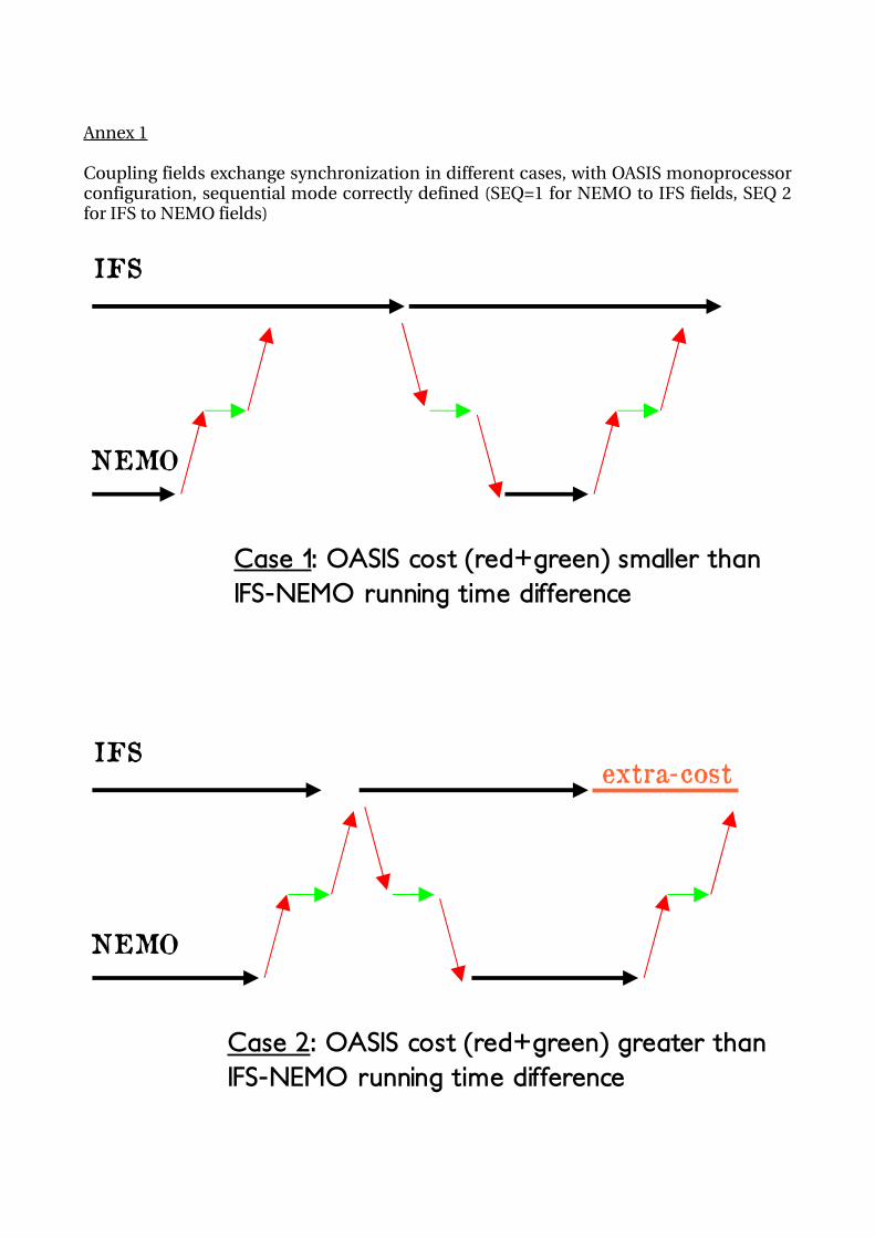
Annex 1

Coupling fields exchange synchronization in different cases, with OASIS monoprocessor configuration, sequential mode correctly defined (SEQ=1 for NEMO to IFS fields, SEQ 2 for IFS to NEMO fields)

IFS

NEMO

Case 1: OASIS cost (red+green) smaller than IFS-NEMO running time difference

IFS

NEMO

Case 2: OASIS cost (red+green) greater than IFS-NEMO running time difference

extra-cost

Annex 2

Modified routines 

master.F90  Call to couplo4_inimpi

sumpini.F90 LCOUPLO4 set to=.true.

couplo4_mix.F90 Change IFS OASIS identifier

couplo4_inimpi.F90couplo4_endmpi.F90

OASIS3 instead of OASIS4 calls

couplo4_definitions.F90 ­Same than previous­Declaration of a new set of variables (Ec­earth namcouple compliant)

couplo4_exchange.F90 ­Same than previous­prism_get/put at any time stepno 3D coupling allowed

Mission #5Nov 16­ Dec 9 2010

Host: Edouard DavinLaboratory: ETH, Zürich (Switzerland)

Main   goal:   Implement   and   validate   an   OASIS4   interface   for   a   regional atmosphere­land model

Main conclusion

A regional atmosphere (COSMO­CLM, DWD) and a land scheme (CLM, NCAR) model have been coupled with OASIS4, at low resolution on a MPP scalar machine (on 100 cores), in order to simplify version updates, allow the use of different time stepping and different grids at different resolutions, and prepare other model components plugging.

The first OASIS4 limitation observed is that OASIS4 does not currently support the CLM original partition; an exchange of the coupling fields through the master process only had to be implemented and will probably be a major bottleneck at higher resolution. Note that the mpp_io library, used for reading and writing restarts in OASIS4, does not support this type of partitioning either. 

Also, a strong slowing down is observed in OASIS4 exchanges when the number of cores used   for   the   component   models   increases,   even   if   these   additional   cores   are   not involved   in   the   coupling   exchanges.   This   problem,   occurring   on   a   particular configuration of grids and partitioning, has to be further investigated.

Model / machine description

COSMO­CLM (here called COSMO)

This regional atmosphere model (v4.8, and its climate version, v11) is used by a large community in several central Europe countries (in which ETHZ). DWD and several other meteorological   agencies   host   the   operational   version   of   the   model.   Grid   size: 109x121x32,   0.44   degrees.   Parallelisation   reaches   100   MPI   tasks   on   the   targeted supercomputer.

CLM

This land scheme is developed at NCAR (v3.5). It is used within the integrated CCLM climate model. Initially, CLM is launched on the same grid that COSMO.

The model is available on CRAY XT5 supercomputer, with 22,128 compute cores (2 six­core   AMD   Opteron   2.4   GHz   Istanbul   processors   per   node),   CRAY   SeaStar   2.2 interconnect.   Peak   performance   of   212  Teraflop/s.  The   machine   is   located   at   CSCS, Manno, Ticino, Switzerland.

Rationale

This user support task proposed to upgrade an existing coupled system with the latest  version of the OASIS coupler. 

The   previous   coupling   (called   integrated   coupling)   gathered   two   models   on   one executable. In this integrated version, CLM is called as a subroutine of COSMO at each time step (sequential coupling). CLM reads input file describing its grid. This input file is written once by COSMO and contains COSMO grid specifications: CLM grid points are COSMO land points. 

CLM and COSMO run on the same processes (used sequentially by one model and the other) which means that CLM and COSMO partitioning differs (CLM processes only land points, COSMO both land and sea points). 

Exchanges between models do not need interpolation (CLM and COSMO land points are located at the same place), just communications between processors (a grid point could be located on different processes during CLM or COSMO computation). 

During the dedicated user support task, OASIS has been evaluated for its capacity to:1. non intrusively be implemented on COSMO and CLM codes2. let user choose the best time step for each model3. launch models on a different number of processors (best number according to 

models distinct scalability)4. investigate possibility of non sequential coupling

Implementation on models

To let user decide which coupling method he wants to use, we kept the possibility to  choose   at   compilation   stage   (by   CPP   key)   between   stand   alone,   existing   integrated coupling method (COSMO calling CLM as a subroutine) or OASIS4 coupling. 

As previously implemented in several models (see NEMO interface, mission #1 and #6), a distinct OASIS4 interface has been written. 

CLM interface

Due   to   a   lack   of   appropriate   option   in   present   OASIS4   partitioning   (see   OASIS development paragraph), coupling fields have to be gathered on the master processor, which  then   communicate   the   coupling   fields   to  COSMO.  Consequences   on  coupling performances has to be evaluated but is obviously an issue for further massively parallel configuration setting.

The possibility to define distinct grids for regional land and atmosphere models implies necessarily  a geographic mismatch between global  domains:  some grid points of   the 

larger grid cannot receive information from the narrowest grid. 

A  strategy to mask the points of the largest subdomain (CLM) falling outside the COSMO domain had to be designed. In the present User Support solution, on a first step, CLM global domain has to be larger than COSMO’s one (CLM latitude and longitude limits have   to   include   COSMO   limits).   The   first   received   field   has   to   be   saved   and   the simulation stopped. A new mask is deduced from this interpolated coupling field and CLM is restarted with this new mask.

Interface routines, driving exchanges with OASIS, are really non intrusive. As usual in such kind of   implementation,   the  off­line  mode routines  which read  forced  fields   in external   files are switched off  and replaced by our coupling fields receiving routines. Coupling fields sending is called as soon as coupling fields are available. 

COSMO interface

The main originality of OASIS interface implementation lies in the possibility to involve a subset of model processes in the coupling, some of them providing no information to land model (all grid points are masked ocean grid points).

At definition stage, prior to any prism_def operation, the number of not masked points is calculated and OASIS initialization routines are called  only if this number is non zero. 

The subroutine  call  of  CLM in COSMO was  easily  changed  for  the  OASIS  interface. Prism_put and prism_get routines (in this order) are called one immediately after the other.   Gather/scatter   operations   needed   in   the   previous   integrated   coupling (interpolation on the whole domain) are now disabled, and communication time is saved at this stage.

Results & performances

Due   to   the   inability   of   the   mpp_io   embedded   output   library   to   support   component processes not involved in the coupling, and thanks to OASIS4 developer Moritz Hanke (DKRZ), an alternate netcdf based parallel output algorithm has been implemented in both interfaces. Received coupling fields are written (and overwritten) at each coupling time step. 

Those fields could be:• used to re­built the CLM adjusted mask (see above)• used to check interpolations validity at implementation stage• compared to arrays exchanged in the previous coupling at validation step.

Two examples of CLM and COSMO received coupled fields, produced after 17 days of simulation are shown on figure 1.

Figure 1: example of COSMO­CLM coupled fields: Infrared on COSMO grid (left) and zonal  wind on CLM grid (right) after 17 days

Geographic discretization of CLM and COSMO can be now totally independent. OASIS performs an interpolation (bicubic) between those two grids, giving the possibility for the  COSMO­CLM  user   to  define,   if  necessary,  a   finer  resolution  on one  or   the  other model. 

Also interesting for performance improvement: each model parallelism can be set at its own optimal level. Saved resources should compensate the fact that both COSMO and CLM models need their own processors 4.

Performances also take benefit of the possibility to set different time step for each model (and coupling time step different from model time steps).

The newly OASIS4 interface allows now, with some additional development, plugging of other models used by COSMO and COSMO­Climate communities. NEMO or ECHAM are possible candidates to complement the regional system model. 

At the end of the user support period, Andy Dobler (Francfort University) starts with us an adaptation (following NEMO example) of the COSMO­OASIS4 interface for OASIS3, to couple COSMO to a Mediterranean NEMO configuration.

Concerning   performances,   figure   2   shows   scalability   of   previous   integrated   coupled model (red curb) and newly implemented OASIS coupled configuration,

(a) using the same time step (240s) on both models and the same coupling frequency (cyan curb)

(b) decreasing down to 1 hour the land model timestep and the coupling frequencies 

4 On CSCS machine, or on every machine where number of processes on one core is limited to one, it is impossible to launch processes of the two executables on the same resources. If models are called sequentially, some resources are wasted while the  processes of one executable waits while  the other model performs its calculations.

(blue curb). 

On   this   graphic,   for   OASIS   based   configurations,   the   resources   number   is   the   total number of cores used for both models and coupler. 12 cores (1 node) are devoted to OASIS,   12   cores   to   CLM   (land   model   calculations   are   much   less   expensive   than   the atmosphere ones) and the number of cores for COSMO varies.

Compared to the previous integrated configuration, a strong slow down is observed due to an increase of the time spent in the coupling communications  (about the same than   the   time   needed   for   one   time   step   calculations).   Surprisingly,   this   slow   down increases when  CLM is parallelised  on more processes, even if these  processes are not involved in the coupling, see CLM interface  section above).

Reducing the coupling time step to 1 hour, OASIS slow down is less visible and curb fits  COSMO   scalability.   For   a   total   number   of   processes   greater   than   75,   response   time becomes even   better  than with the previous  integrated coupling approach.  But  it   is important to realize here that this reduction in the response time is partially due to the fact that CLM is called less often, and changes on model results have to be evaluated to  conclude if this configuration is or not equivalent to the existing one.

Figure 2: COSMO­CLM coupled model performances on CRAY XT5 for different coupling interfaces

OASIS4 developments

Exploring OASIS4 coupler capacity to fully satisfy the community needs is one of the important OASIS Dedicated User Support goal.

A strong day by day interaction with OASIS4 developers allowed us to  identify, address or bypass related issues. 

1D partitioning

A first analysis of CLM partitioning let us identify a restriction on OASIS use for some rectangular grids5.  CLM calculations only occurs on land points and are independent: those   points   can   be   considered   as   a   1D   vector,   split   onto   processes   without   any geographic consideration (same kind of partitioning could be observed on models like LIM sea ice or SURFEX land scheme).

The   temporary   solution   implemented   (exchange   of   gathered   field   on   master processor) can be considered as a major bottleneck for further high resolution (and massively parallel) CLM configuration.

Masked partitions

In   our   particular   partitioning,   some   subdomains   are   not   involved   in   the   coupling because they don’t intersect any unmasked points (COSMO) or also because they are not the master processor (CLM).

During coupling definition phase (halo detection), we identified some OASIS incapacity to consider separately MPI communications of process involved in the coupling and MPI waiting state in which non involved process lies. This problem has been addressed on­the­fly and solved by OASIS developers.

 Mpp_io library

To validate coupling fields,  OASIS debug outputs have been turn on but without any success, because the  mpp_io library seemed to be unable to support a configuration into which some processes are not involved in the coupling and therefore do not write any part of the coupling fields in the output file. 

This   restriction   also   concerns   coupling   restart   read/write   operations   and   therefore prevented us to further test a   parallel  execution of the land and atmosphere models (instead of their sequential execution as reported here). 

To   visualize the coupling fields, a  workaround solution has been  suggested by OASIS team and implemented, each process calling in turn Netcdf within model interfaces (see 

5 For the moment, OASIS assumes that (i plus 1) and (i minus 1) points are geographically neighbours, which is not the case on our partitioning. A non trivial development is needed to address this issue. 

above in Results & performances).

Scalability issues

As mentioned above, the most important problem identified during this support task concerns  abnormal coupling slow down  and its  increase with the number of model processes, even when those processes are not involved in the coupling (see table 3).

CRAY XT5 (12 cores/node) SGI Altix (8 cores/node)

OASIS CLM COSMO Comm(s) OASIS CLM  COSMO  Comm(s)

12 12 36 0.20 8 8 32 0.01

12 12 60 0.30 8 8 64 0.02

12 12 96 0.37 8 8 128 0.05

12 12 132 0.43

12 12 60 0.30 8 8 64 0.02

12 36 60 0.33 8 64 64 0.53

12 60 60 0.56 8 128 64 1.80Table 3: mean duration of a total OASIS coupling sequence

Further investigations are needed to identify which service can be at the origin of the slowing down. A toy model is implemented to try to reproduce the problem, without success.  This  could suggest   that  an  interaction between model  calculations and MPI communication could occur in this configuration (memory ? MPI buffers ?)

The coupled model has been  ported on an SGI Altix platform and the same performance tests processed (4 right columns of the table 3). Even if calculations are achieved during the same time with about the same number of processors, the time spent within OASIS calculations and communications is slower.

But again, if we increase the number of CLM processors (not involved in the coupling), this duration amazingly increases. This identical behaviour on both machines suggests that the particular CSCS MPI installation on the CRAY machine (or some default MPI characteristics) is not at the origin of the noticed slowing down6. 

Needed improvements

On top of those OASIS improvements, some additional tasks have to be tackled to be able to guarantee an functional and efficient coupling between COSMO and CLM models.

6 Various code instrumentation (TAU & Scalasca) have been tested to try to identify the bottleneck. TAU profiling only reveals MPI_Wait or MPI_Barrier excessive durations. Scalasca full tracing was not possible to   produce   on   our   MPI   MPMD   configuration   (the   software   new   version   could   address   the   problem, contacts are ongoing with Jean Guillaume Piccinalli from CSCS).

Needed on every coupled system exchanging fluxes, conservative interpolation has to be tested.

Then,   coupled   fields   have   to   be   compared   with   those   of   integrated   coupling. Characteristics   of   those   fields   have   to   be   checked   when   coupling   field   frequency decreases.   A   special   care   should   be   taken   on   the   behaviour   of   exchange   coefficient, recomputed   in   the   atmosphere   when   fluxes   are   changed   by   land   model.   Models characteristics such as diurnal cycle or long term means should be compared.

Finally, we hope that scalability tests with higher definition (operational) models could begin, to possibly investigate limitations of OASIS4 parallelism with such configuration.

Mission #6Feb 28­ Mar 25 2011

Hosts: Guillaume Samson & Sébastien MassonLaboratory: LOCEAN, Paris (France)

Main   goal:   Implement   and   validate   an   OASIS4   interface   for   a   regional atmosphere­ocean model

Main conclusion

Even though model interfaces have been successfully adapted from OASIS3 to OASIS4 in  the WRF and NEMO component  models,   too many issues  remains  to  attribute a scientific   validity   to   the   coupling:   impossibility   to   use   OASIS   reading   and   writing mechanism for coupling restart files, issue with masked partitions, non completion of the run with different interpolations above a certain number of cores. 

In fact, even if OASIS4 computational cost appears significantly low (less than 1% of the total   duration),   failures   on   parallel   interpolation   weight   calculation   forbid   to   fully validate coupler scalability at serious level of parallelism for the different interpolations (e.g. more than 128 resources for the nearest neighbour interpolation).

Model / machine description

WRFThe NCAR regional atmosphere model (v3.2.1) is used by a large community in several countries. This easy to use model becomes more and more popular on several European laboratories. Grid size: 469x256x28. Parallelisation reaches 128 MPI tasks on the targeted supercomputer.

NEMOThe well known European ocean model is embedded on most of the continental CMIP5 coupled systems. We used a regional configuration (Indian ocean) developed at LOCEAN with the 3.3 version. Grid size: 463x273x46. No parallelism needed up to 24 MPI tasks.

The model is available on IBM Power6 supercomputer, with 3,584 compute cores (16 dual­core IBM P6 4.7 GHz processors per node), Infiniband x4 DDR interconnect. Peak performance of 67.3 Teraflop/s. The machine belongs to IDRIS CNRS supercomputing centre, Orsay, France.

Rationale

This user support task proposes to adapt interfaces of an existing coupled system (based 

on OASIS3) to be able to use the new version of the OASIS coupler.

This OASIS4 coupling will be evaluated for its capacity to:1. be operational without any important interface modification  2. provide a very simple interpolation (WRF and NEMO spatial discretizations are 

very close so a nearest neighbour interpolation is satisfactory)3. address   coupler   scalability   issues   with   highly   parallelized   configuration   (high 

number   of   process­to­process   communications   during   coupling   field   message passing)

OASIS interfaces

NEMO interface:

This work starts from developments produced during #1 OASIS User support mission completed last year on NEMO model, based on ORCA global configuration. It includes corrections added during high resolution ARPEGE­NEMO coupling tests (IS­ENES WP8­JRA2).

Slight improvements have been made on existing interface:

1.   possibility   to   switch   off   a   process   when   all   its   grid   points   are   masked   (“masked partition”). 2 options: 

• the   model   is   launched   only   with   subdomains   containing   at   least   some   non masked points (optional on NEMO only)

• the model is launched on all subdomains but coupling is not effective on masked partitions (only prism_init, prism_init_comp, prism_enddef and prism_terminate OASIS primitives are called by the corresponding processes).

2. pseudo­parallel coupling field writing (thanks to Moritz Hanke, DKRZ). To compensate for OASIS IO deficiency, coupling field is written immediately after receiving. Writing is pseudo parallel, which means that every process writes its subdomain in turn (and not simultaneously).

Same features has been implemented on WRF interface.

WRF interface:

Following NEMO implementation, a module_cpl_oasis4.F has been written, to be able to call the same wrapping procedures with OASIS3 (module_cpl_oasis3.F):

cpl_prism_init: initialization of coupled mode communication cpl_prism_define: definition of grid and fields cpl_prism_snd: snd out fields in coupled mode cpl_prism_rcv: receive fields in coupled mode cpl_prism_finalize: finalize the coupled mode communication cpl_prism_update_time: update date sent to OASIS 

This last routine only has to be called when OASIS4 coupling is active. The others are  called in both configuration (OASIS3 or OASIS4 coupling).

On both WRF and NEMO interfaces, basic timing measure (using MPI_Wtime) has been implemented:

1. after last coupling field receive and before first coupling field receive.2. before last coupling field send on (slowest model) WRF interface and after  last 

receive on (fastest model) NEMO interface.

Two shell scripts collect information on standard output files and provide:

1. total time spent by model for calculation. This information is needed to be able to balance processor allocation.

2. time spent for WRF to NEMO coupling fields communications and interpolation (6 coupling fields).

OASIS improvements

Restart

OASIS  coupling  restart   read/write   is   based  on   mpp_io   library   (same   library  used  for coupling restart read/write in OASIS3).

Issues occurs frequently on mpp_io with any kind of non regular grid or partitioning (see report on mission #2). This time, a deadlock appears on simple NF_GET_VARA_DOUBLE function.   A   switch   from   standard   netcdf   calls   to   p­netcdf   (parallel   netcdf)   was   not successful (error on reading arrays shape declaration).

Moreover, we found two error sources that could easily mislead inattentive programmers and cause large waste of time:

1. A   bad   declaration   of   time   bounds   (not   verified   by   OASIS)   could   leads   to   a mismatch between restart file netcdf read (that should occur at time step 0) and effective information exchange (that is delayed at coupling time step number 2)

2. LAG declaration must not be done in second (as OASIS3 required it) or, in that case, a deadlock (for a quite difficult reason to identify) will occur at 2nd coupling time step. Here, a specific error would be appreciated.

Simplification   of   restart   read/write   strategy   is   urgently   required.   Mpp_io   library substitution should be a 2011 priority for OASIS developers.

Masked partitions

On a broad range of model types (surfaces, ocean, etc.), calculations take place only on a subset of the grid points. When parallelism increases, some partition could be made up of masked points only. 

For a subdomain composed entirely with masked points, it was observed that  calling the ordinary   API   routines   (prism_def_grid,   prism_set_corners,   prism_set_mask, 

prism_def_partition, prism_set_points, prism_def_var) lead to a deadlock.

We therefore   decided to switch off  coupling on these masked partitions (see NEMO interface paragraph).

For example, on figure 3 (left),  NEMO parallelism along X (longitude) is 6, parallelism along Y (latitude) is 4, but total number of allocated processors is 23 (no calculation over  Australia region).

Figure 3: example of NEMO­WRF­OASIS4 coupled fields: non solar on NEMO grid (left), 1 uncoupled partitions (white box)

and SST on WRF grid (right), 11 uncoupled partitions 

Implementation of our coupling interfaces must take into account those particularities (see “OASIS interfaces” paragraph). One of the difficulties is the necessity to synchronize involved and masked processors.

Unfortunately, possibility to switch off partition have side effect on parallel interpolation functionality   :   target/source   point   matching   research   could   not   be   done   on   empty partitions. 

Consequence could be the non definition of some values (particularly near coastline and domain boundaries). It was observed with the “nearest neighbour” (NN) interpolation. Use of bilinear or bicubic interpolation leads to deadlock, when parallelism increases (up to #128). NN is preferred to those two other interpolations.

Moreover, WRF and NEMO discretization are the same, except on northern hemisphere were NEMO latitude circles begin to fold due to pole duplication: in this case, NN is the most appropriate interpolation.  

To bypass problem of non definition near coastline and domain boundary, we decided to choose   first   strategy   of   masked   partition   switching   off:   model   is   launched   on   all subdomains but coupling is not effective if all grid point of the domain are masked (see  NEMO interface paragraph).

Nearest neighbour interpolation

The interpolation we prefer to use at  this stage suffers from the impossibility to find neighbours on source grid if target grid point centre position does not belong to a non masked   source   grid   point   area.  This   occurs   near   masks,   masked   partitions   or   whole domain boundaries.

To compensate for this default,  a simplified and domain restricted nearest neighbour algorithm has been implemented on model interfaces.

Results/performances

Restitution time comparison between coupled model and slowest model in forced mode (WRF) do not show any extra cost.

Resources # NEMO­WRF­OASIS4 WRF stand alone

18­6­1 1220 1220

121­6­1 330 330Table 4: restitution time (for 1 simulated day) on coupled and forced mode (s). On forced  

mode, WRF has the same resources # than in coupled mode.

Evaluated OASIS cost  remains significantly  slower (less than 1%) than computational time.  This   cost   increases   with   model   parallelism   but   could   be   reduced   with   coupler parallelism.

WRF­NEMO resources # 1 OASIS4 6 OASIS4

18­6 0.025 / 50.9 (0.05%)

52­6 0.107 / 25.0 (0.42%) 0.027 / 25.0 (0.10%)

110­12 0.119 / 15.4 (0.77%) 0.065 / 15.4 (0.42%)Table 5: estimated OASIS time / model restitution time (ratio %). In seconds. OASIS time 

represents communication and interpolation time needed for 6 coupling field exchanges. 

Unfortunately,   unidentified   issues   occurring   during   neighbour   identification   phase (prism_enddef   routine,   parallel   interpolation   weight   calculation)   at   higher   level   than #128 prohibit more serious test on OASIS4 scalability.