Embed Size (px)
Citation preview

ISEN 315Spring 2011
Dr. Gary Gaukler

Demand Uncertainty
How do we come up with our random variable of demand?
Recall naïve method:

Demand Uncertainty

Demand Uncertainty and Forecasting
Using the standard deviation of forecast error:
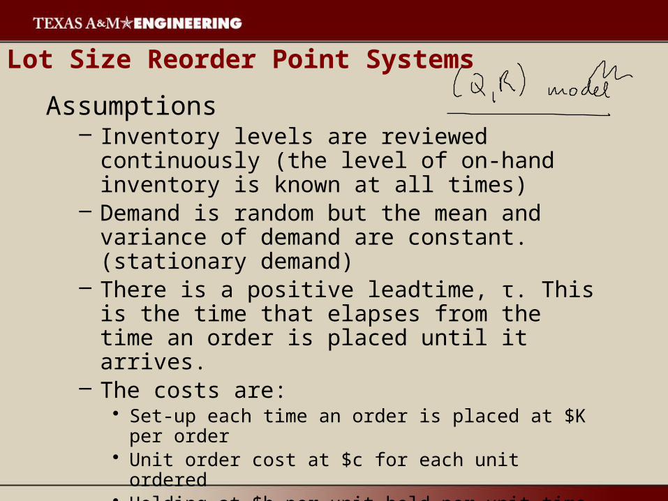
Lot Size Reorder Point Systems
Assumptions– Inventory levels are reviewed continuously (the
level of on-hand inventory is known at all times)– Demand is random but the mean and variance of
demand are constant. (stationary demand)– There is a positive leadtime, τ. This is the time that
elapses from the time an order is placed until it arrives.
– The costs are: • Set-up each time an order is placed at $K per order• Unit order cost at $c for each unit ordered• Holding at $h per unit held per unit time ( i. e., per year)• Penalty cost of $p per unit of unsatisfied demand

The Inventory Control Policy
• Keep track of inventory position (IP)• IP = net inventory + on order• When IP reaches R, place order of size Q
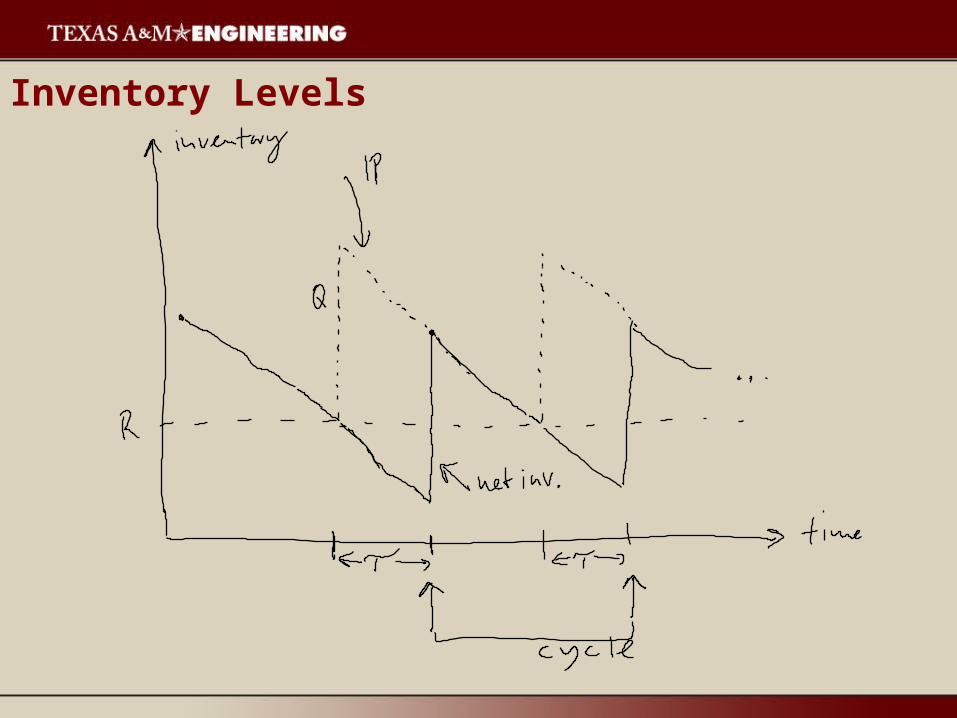
Inventory Levels

Describing Demand
• The response time of the system in this case is the time that elapses from the point an order is placed until it arrives. – The uncertainty that must be protected against is
the uncertainty of demand during the lead time. • Assume that D represents the demand during
the lead time and has probability distribution F(t).
• Although the theory applies to any form of F(t), we assume that it follows a normal distribution for calculation purposes.

Decision Variables
• Basic EOQ model:– Single decision variable Q
• Q,R model:– Q and R interdependent decision variables.
Essentially, R is chosen to protect against uncertainty of demand during the lead time, and Q is chosen to balance the holding and set-up costs
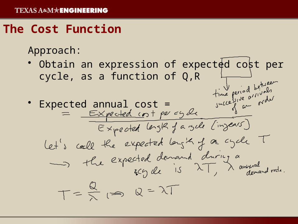
The Cost Function
Approach:• Obtain an expression of expected cost per cycle, as a
function of Q,R
• Expected annual cost =

The Cost Function
• Holding cost:
• Setup cost:
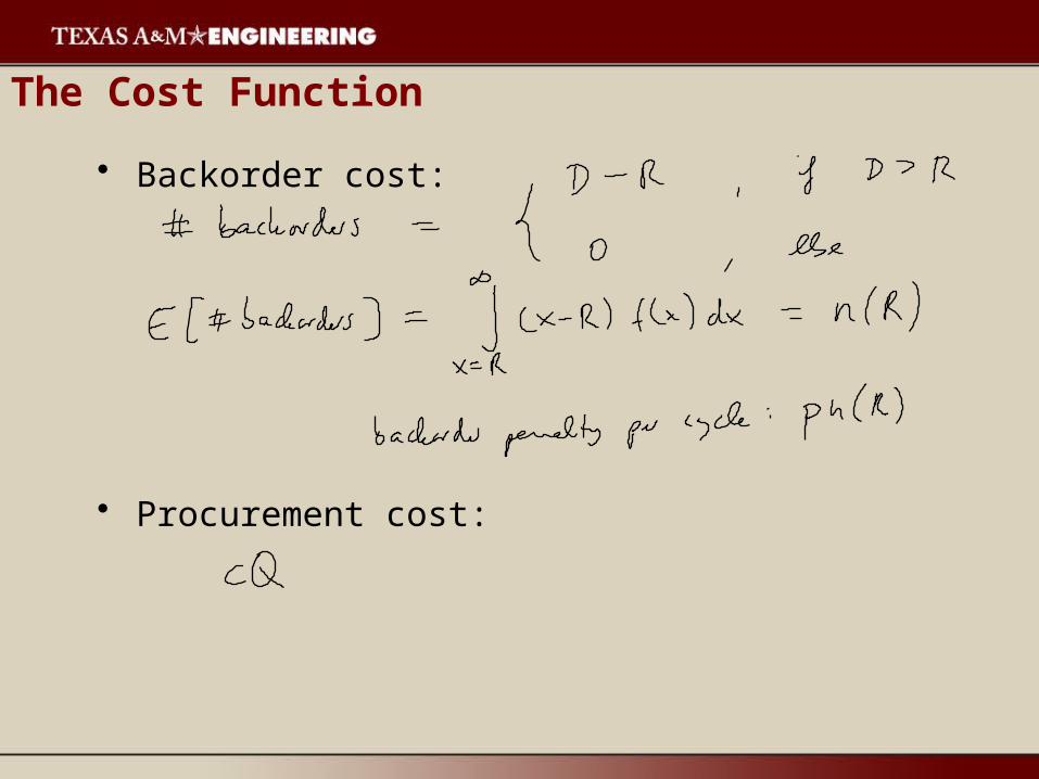
The Cost Function
• Backorder cost:
• Procurement cost:

The Cost Function
• Expected cost per cycle:
• Expected annual cost:
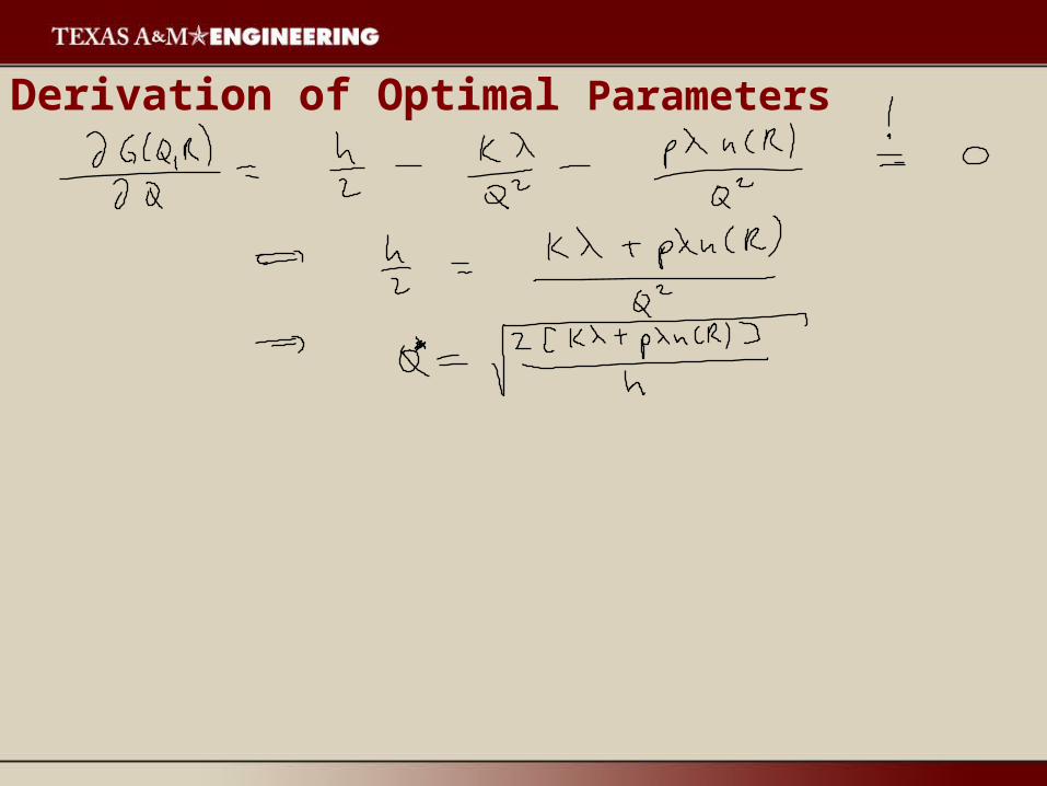
Derivation of Optimal Parameters

Derivation of Optimal Parameters

Review
Optimal (Q,R):

Solution Procedure
• The optimal solution procedure requires iterating between the two equations for Q and R until convergence occurs (which is generally quite fast).
• A cost effective approximation is to set Q=EOQ and find R from the second equation.
• In this class, we will use the approximation.
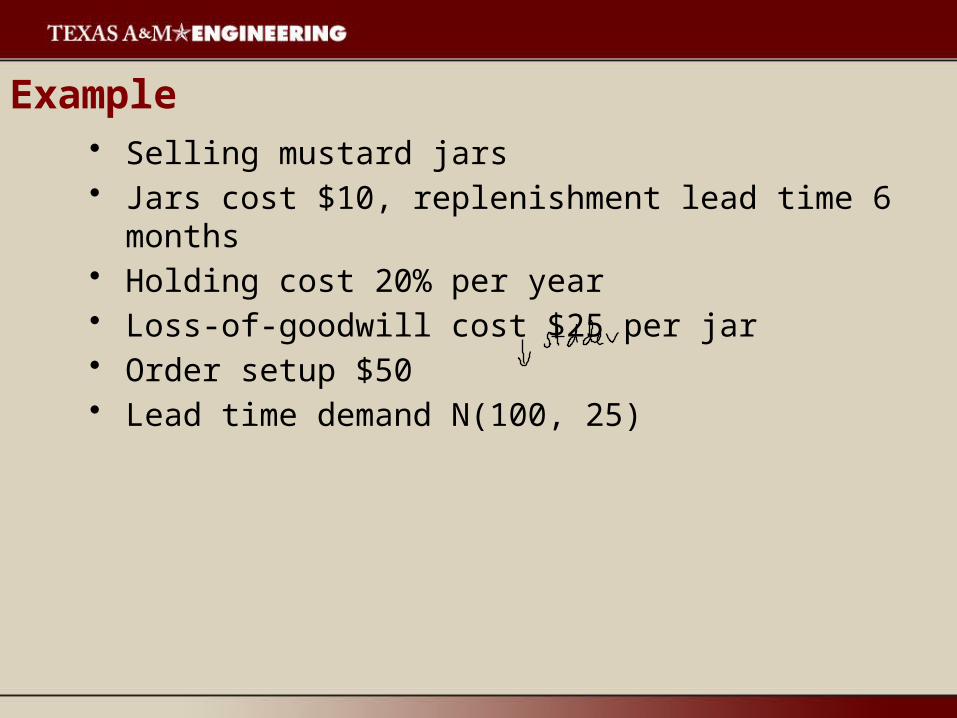
Example• Selling mustard jars• Jars cost $10, replenishment lead time 6 months• Holding cost 20% per year• Loss-of-goodwill cost $25 per jar• Order setup $50• Lead time demand N(100, 25)

Example

Example