/* push dates to agree with a most recent sample date at endTime and oldest sample date is startTime */

/* will fail if used on contempory samples */

void CoalescentTree::pushTimesBack(double startTime, double endTime) {

tree<Node>::iterator it, jt;

double presentTime = getPresentTime();

if (startTime < endTime) {

// STRETCH OR SHRINK //////////////

ISC-3133 Introduction to Scientific Computingusing C++Peter Beerli

Professor

Department of Scientific Computing

Office: 150-T Dirac Science Library

Phone: (850) 559 9664

Email: beerli at fsu dot edu

Web: http://people.sc.fsu.edu/~pbeerli

© http://abstrusegoose.com/275

Course Objectives:

• Identify the components of scientific computing;

• Identify standard problems in scientific computing;

• Implement basic algorithms for standard problems in computational science using the programming language Java.

• Write, debug, and verify computer codes;

• Output results of computer simulations on a meaningful manner.

Course Description:

This course introduces you to the science of computations. Algorithms for standard problems in computational science are presented. The basics of the object-oriented programming language C++ are taught to facilitate the implementation of algorithms.

Grading Policy:

The student’s grade for the course will be based upon classwork, homework, and a final capstone project. This work is weighted as follows:

• Classwork/Quizzes (weekly) - 10%

• Assignments (weekly to biweekly: description, code) - 50%

• Capstone Project (project description, code, presentation) - 40%

I. Components of Scientific Computing

II. A simple example (actually two) - Using a Monte Carlo approach to approximate problems 1. UNIX basics 2. Netbeans IDE: an integrated development environment for C++

programming 3. Introduction to C++ 4. Algorithm development 5. Program testing and documentation 6. Visualization and analysis of results

III. Solving a non-linear equations 1. Description of problem and some simple algorithms 2. Iterative methods, required accuracy of result 3. Implementation of the Bisection method 4. Program testing and documentation

IV.Object oriented programming concepts in detail using the non-linear equation problem and implementing more methods

1. Encapsulation 2. Inheritance 3. Polymorphism 4. Abstract classes and datatypes

V. Operations on vectors and matrices 1. Development of general functionality that is usable in many places 2. Vector and Matrix operations 3. Vector norms 4. Concurrency and parallel processing of such calculations using C++

VI. Polynomial interpolation of data 1. Description of problems and (biological) applications 2. Algorithms: Lagrangian interpolation in detail 3. Implementation to fit a set of data 4. Piecewise interpolation 5. Implementation and visualization of of piecewise interpolation

VII.Solving ordinary differential equations systems 1. Description of problem: Lotka-Volterra Predator-Prey system 2. Algorithms 3. How to use functions from other libraries 4. How to assess correctness of program 5. Visualization of results

VIII. Markov chain Monte Carlo method 1. Description of method 2. Example application 3. Implementation 4. Testing and visualization of results

IX.Capstone project presentation

ContentsWe have a total of 17 weeks of instruction, we will spend about two weeks per topic. Computational science [or Scientific Computing]

From Wikipedia, the free encyclopedia

Not to be confused with computer science.

Computational science (or scientific computing) is the field of study concerned with constructing mathematical models and quantitative analysis techniques and using computers to analyse and solve scientific problems. In practical use, it is typically the application of computer simulation and other forms of computation to problems in various scientific disciplines.The field is distinct from computer science (the study of computation, computers and information processing). It is also different from theory and experiment which are the traditional forms of science and engineering. The scientific computing approach is to gain understanding, mainly through the analysis of mathematical models implemented on computers.

Scientists and engineers develop computer programs, application software, that model systems being studied and run these programs with various sets of input parameters. Typically, these models require massive amounts of calculations (usually floating-point) and are often executed on supercomputers or distributed computing platforms.

Numerical analysis is an important underpinning for techniques used in computational science.

Computer science or computing science (sometimes abbreviated CS) is the study of the theoretical foundations of information and computation, and of practical techniques for their implementation and application in computer systems.[1][2][3][4] It is frequently described as the systematic study of algorithmic processes that create, describe, and transform information.

Computer Science

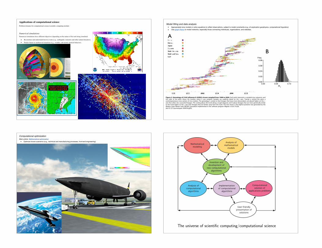
Applications of computational scienceProblem domains for computational science/scientific computing include:

Numerical simulationsNumerical simulations have different objectives depending on the nature of the task being simulated:

■ Reconstruct and understand known events (e.g., earthquake, tsunamis and other natural disasters).■ Predict future or unobserved situations (e.g., weather, sub-atomic particle behavior).

Model fitting and data analysis■ Appropriately tune models or solve equations to reflect observations, subject to model constraints (e.g. oil exploration geophysics, computational linguistics)■ Use graph theory to model networks, especially those connecting individuals, organizations, and websites.

combined -- 5

Migrate debug 4.0: (http://popgen.sc.fsu.edu) [program run on 23:39:37]

Bayesian Analysis: Posterior distribution over all loci

Freq

Θ1

0.00

0.02

0.04

0.06

0.08

0.00 0.05 0.10

Contacts between regions produce migration events, which wedepict as shifts in color in the virus genealogy (Figure 2). Thegenealogy shows that migration events between major geographicregions are uncommon, and thus the virus is not well-mixedamong regions. Generally, we observe genetic diversification overthe course of a regional epidemic, after which time few, if any,lineages persist. Local persistence appears in a genealogy as a sidebranch present in the same region over multiple seasons. It is clearfrom the influenza tree that this pattern is rare, suggesting lineages

of influenza do not often persist from season to season withintemperate regions.While a general lack of local persistence is consistent with

previous results [2,3], we find that contrary to previous hypotheses[3,4] seasonal epidemics in temperate regions can seed futureepidemics around the world. For example, we find that the 1998–1999 USA epidemic seeds two major influenza lineages. The firstof these lineages appears as a temperate lineage that circulatespredominantly in Europe, Oceania, South America and the USA.This lineage persists for *5 years. The second lineage is part ofthe trunk of the genealogy; it migrates from the USA into China,where it persists from 2000 to 2003. After 2003, this lineagespreads to the rest of the world. Thus, we find that globalpersistence is aided by metapopulation structure in which infectionis dynamically sustained through contact between regions ofdifferent seasonality.

Trunk reconstructionAt any given moment there is a strain of influenza that will

eventually, through natural selection and genetic drift, become theprogenitor of all future influenza strains. Looking backward intime, this is equivalent to the statement that all current strains ofinfluenza share a common ancestor at some time in the past. Thisprogenitor strain corresponds to the trunk of the influenzagenealogy (Figure 2) and is where historically relevant evolutionoccurs; only mutations that occur along the trunk are maintainedindefinitely, while mutations that occur along other branches willeventually be lost. Still, mutations to side branches may have

Table 1. Means and 95% confidence intervals acrossresampled replicates for the total rates of immigration from allother regions and emigration to all other regions for eachregion measured in terms of migration events per lineage peryear.

Immigration Emigration

China 0.79 (0.49, 1.18) 1.05 (0.59, 1.73)

Europe 0.70 (0.52, 0.90) 0.59 (0.33, 1.06)

Japan 0.76 (0.57, 0.98) 0.51 (0.29, 1.14)

Oceania 1.27 (0.91, 1.81) 0.55 (0.31, 0.91)

South America 0.47 (0.42, 0.52) 0.30 (0.21, 0.38)

Southeast Asia 0.85 (0.52, 1.15) 0.91 (0.49, 1.64)

USA 0.70 (0.44, 1.11) 1.62 (0.91, 2.33)

doi:10.1371/journal.ppat.1000918.t001

Figure 2. Genealogy of 2165 influenza A (H3N2) viruses sampled from 1998 to 2009. Each point represents a sampled virus sequence, andthe color of the point shows the location where it was sampled. Samples are explicitly dated on the x-axis. Tracing a vertical line gives acontemporaneous cross-section of virus isolates. The genealogy is sorted so that lineages that leave more descendants are placed higher on the y-axis than other, less successful lineages. This sorting places the trunk along a rough diagonal, and it places lineages that are more genetically similarto the trunk higher on the y-axis than lineages that are farther away from the trunk. The tree shown is the highest posterior tree generated by theMarkov chain Monte Carlo (MCMC) procedure implemented in the software program Migrate v3.0.8 [14,20].doi:10.1371/journal.ppat.1000918.g002

Global Migration Dynamics of Influenza A

PLoS Pathogens | www.plospathogens.org 3 May 2010 | Volume 6 | Issue 5 | e1000918

A

B

Computational optimizationMain article: Mathematical optimization■ Optimize known scenarios (e.g., technical and manufacturing processes, front-end engineering).

!"#$%&$'#()*+,$#"#(-.-'/(0/&

"/*1-'/("

2/3,1-.-'/(.*"/*1-'/(0/&

.,,*'4.-'/("0,$/5*#3"

63,*#3#(-.-'/(/&04/3,1-.-'/(.*

.*7/$'-83"

9(.*+"'"0/&4/3,1-.-'/(.*.*7/$'-83"

6(:#(-'/(0.())#:#*/,3#(-0/&

(#;04/3,1-.-'/(.*.*7/$'-83"

9(.*+"'"0/&3.-8#3.-'4.*

3/)#*"

<.-8#3.-'4.*3/)#*'(7

The universe of scientific computing/computational science

in this course, ....

• we are mainly interested in implementing computational algorithms.

• we will use C++ to implement these algorithms

• we will learn the basics of C++ in the context of basic methods in scientific computing such as

★approximate integrals:

★solving a single nonlinear equation, e.g. find xsuch that

★ interpolating or fitting data, e.g. find a line

★vector and matrix operations

★solving simple differential equation, numerically

• We will visualize some of the results with GNUPLOT or other visualization methods.

Z b

af(x)dx

x = sin x

y = mx+ b

A�x = �y

dydt = e�gt, y(0) = y0

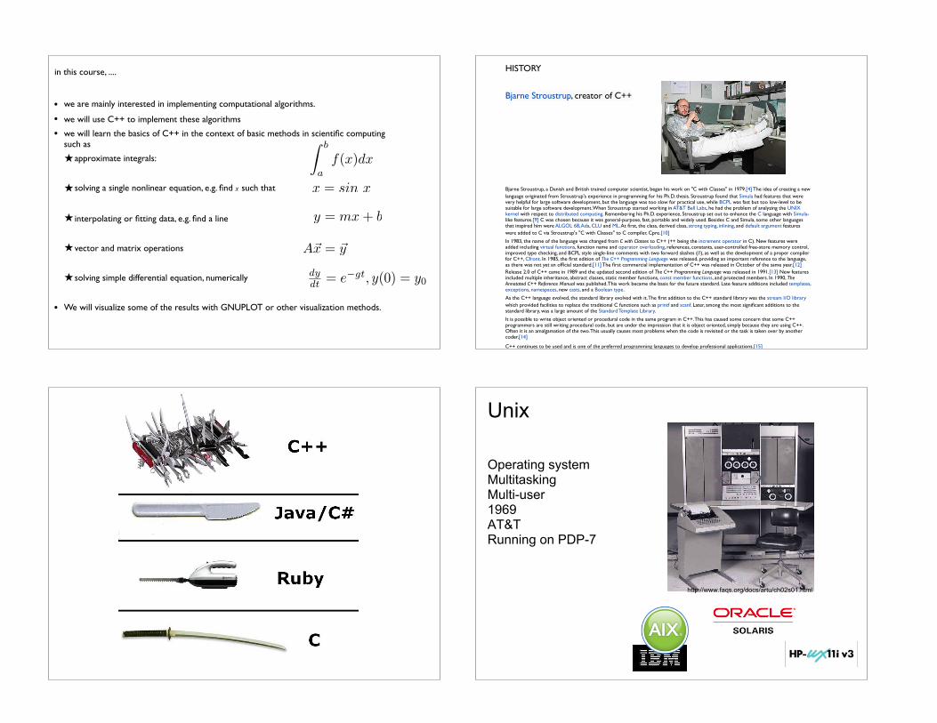
HISTORY

Bjarne Stroustrup, creator of C++

Bjarne Stroustrup, a Danish and British trained computer scientist, began his work on "C with Classes" in 1979.[4] The idea of creating a new language originated from Stroustrup's experience in programming for his Ph.D. thesis. Stroustrup found that Simula had features that were very helpful for large software development, but the language was too slow for practical use, while BCPL was fast but too low-level to be suitable for large software development. When Stroustrup started working in AT&T Bell Labs, he had the problem of analyzing the UNIX kernel with respect to distributed computing. Remembering his Ph.D. experience, Stroustrup set out to enhance the C language with Simula-like features.[9] C was chosen because it was general-purpose, fast, portable and widely used. Besides C and Simula, some other languages that inspired him were ALGOL 68, Ada, CLU and ML. At first, the class, derived class, strong typing, inlining, and default argument features were added to C via Stroustrup's "C with Classes" to C compiler, Cpre.[10]

In 1983, the name of the language was changed from C with Classes to C++ (++ being the increment operator in C). New features were added including virtual functions, function name and operator overloading, references, constants, user-controlled free-store memory control, improved type checking, and BCPL style single-line comments with two forward slashes (//), as well as the development of a proper compiler for C++, Cfront. In 1985, the first edition of The C++ Programming Language was released, providing an important reference to the language, as there was not yet an official standard.[11] The first commercial implementation of C++ was released in October of the same year.[12] Release 2.0 of C++ came in 1989 and the updated second edition of The C++ Programming Language was released in 1991.[13] New features included multiple inheritance, abstract classes, static member functions, const member functions, and protected members. In 1990, The Annotated C++ Reference Manual was published. This work became the basis for the future standard. Late feature additions included templates, exceptions, namespaces, new casts, and a Boolean type.

As the C++ language evolved, the standard library evolved with it. The first addition to the C++ standard library was the stream I/O library which provided facilities to replace the traditional C functions such as printf and scanf. Later, among the most significant additions to the standard library, was a large amount of the Standard Template Library.

It is possible to write object oriented or procedural code in the same program in C++. This has caused some concern that some C++ programmers are still writing procedural code, but are under the impression that it is object oriented, simply because they are using C++. Often it is an amalgamation of the two. This usually causes most problems when the code is revisited or the task is taken over by another coder.[14]

C++ continues to be used and is one of the preferred programming languages to develop professional applications.[15]

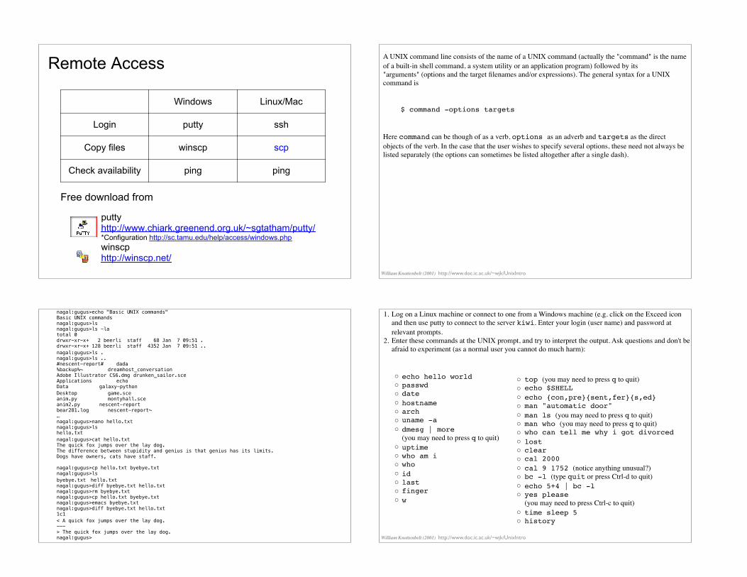
8QL[

2SHUDWLQJ�V\VWHP0XOWLWDVNLQJ0XOWL�XVHU����$775XQQLQJ�RQ�3'3��

KWWS���ZZZ�IDTV�RUJ�GRFV�DUWX�FK��V���KWPO

KWWS���DFDGHPLF�XGD\WRQ�HGX�6DYHULR3HUXJLQL�FRXUVHV�FSV����OHFWXUHBQRWHV�81,;SKLOR�KWPO

(YROXWLRQ�RI�8QL[�DQG�8QL[�OLNH�26

)URP�:LNLSHGLD

/LQX[

8QL[�OLNH�IUHH�2SHUDWLQJ�V\VWHP�����a/LQXV�7RYDOGV��PDQ\�RWKHUV/LQX[�GLVWULEXWLRQƔ 8QL[�OLNH�RSHUDWLQJ�V\VWHP�EDVHG�RQ��/LQX[�NHUQHO��

8VHG�E\�DOO�RI�ZRUOG�WRS����6XSHUFRPSXWHUV�-XQH�������

�

2SHUDWLQJ�6\VWHP

5HPRWH�$FFHVV

:LQGRZV /LQX[�0DF

/RJLQ SXWW\ VVK

&RS\�ILOHV ZLQVFS VFS

&KHFN�DYDLODELOLW\ SLQJ SLQJ

�SXWW\KWWS���ZZZ�FKLDUN�JUHHQHQG�RUJ�XN�aVJWDWKDP�SXWW\� &RQILJXUDWLRQ�KWWS���VF�WDPX�HGX�KHOS�DFFHVV�ZLQGRZV�SKSZLQVFSKWWS���ZLQVFS�QHW�

)UHH�GRZQORDG�IURP

A UNIX command line consists of the name of a UNIX command (actually the "command" is the name of a built-in shell command, a system utility or an application program) followed by its "arguments" (options and the target filenames and/or expressions). The general syntax for a UNIX command is

    $ command -options targets

Here command can be though of as a verb, options as an adverb and targets as the direct objects of the verb. In the case that the user wishes to specify several options, these need not always be listed separately (the options can sometimes be listed altogether after a single dash).

William Knottenbelt (2001) http://www.doc.ic.ac.uk/~wjk/UnixIntro

nagal:gugus>echo "Basic UNIX commands" Basic UNIX commands nagal:gugus>ls nagal:gugus>ls -la total 0 drwxr-xr-x+ 2 beerli staff 68 Jan 7 09:51 . drwxr-xr-x+ 128 beerli staff 4352 Jan 7 09:51 .. nagal:gugus>ls . nagal:gugus>ls .. #nescent-report# dada %backup%~ dreamhost_conversation Adobe Illustrator CS6.dmg drunken_sailor.sce Applications echo Data galaxy-python Desktop game.sce anim.py montyhall.sce anim2.py nescent-report bear281.log nescent-report~ … nagal:gugus>nano hello.txt nagal:gugus>ls hello.txt nagal:gugus>cat hello.txt The quick fox jumps over the lay dog. The difference between stupidity and genius is that genius has its limits. Dogs have owners, cats have staff.

nagal:gugus>cp hello.txt byebye.txt nagal:gugus>ls byebye.txt hello.txt nagal:gugus>diff byebye.txt hello.txt nagal:gugus>rm byebye.txt nagal:gugus>cp hello.txt byebye.txt nagal:gugus>emacs byebye.txt nagal:gugus>diff byebye.txt hello.txt 1c1 < A quick fox jumps over the lay dog. --- > The quick fox jumps over the lay dog. nagal:gugus>

1. Log on a Linux machine or connect to one from a Windows machine (e.g. click on the Exceed icon and then use putty to connect to the server kiwi. Enter your login (user name) and password at relevant prompts.

2. Enter these commands at the UNIX prompt, and try to interpret the output. Ask questions and don't be afraid to experiment (as a normal user you cannot do much harm):

◦ echo hello world◦ passwd◦ date◦ hostname◦ arch◦ uname -a◦ dmesg | more

(you may need to press q to quit)◦ uptime◦ who am i◦ who◦ id◦ last◦ finger◦ w

◦ top (you may need to press q to quit)◦ echo $SHELL◦ echo {con,pre}{sent,fer}{s,ed}◦ man "automatic door"◦ man ls (you may need to press q to quit)◦ man who (you may need to press q to quit)◦ who can tell me why i got divorced◦ lost◦ clear◦ cal 2000◦ cal 9 1752 (notice anything unusual?)◦ bc -l (type quit or press Ctrl-d to quit)◦ echo 5+4 | bc -l◦ yes please

(you may need to press Ctrl-c to quit)◦ time sleep 5◦ history

William Knottenbelt (2001) http://www.doc.ic.ac.uk/~wjk/UnixIntro

http://en.wikipedia.org/wiki/Comparison_of_text_editors

UNIX editors

Most common basic UNIX editors

Pipelines • stdin

• stdout

• stderr

cat hello.txt | sort | uniq

cat hello.txt | grep "dog" | grep -v "cat"

To redirect standard output to a file instead of the screen, we use the > operator:

    $ echo hello     hello     $ echo hello > output     $ cat output     hello

In this case, the contents of the file output will be destroyed if the file already exists. If instead we want to append the output of the echo command to the file, we can use the >> operator:

    $ echo bye >> output     $ cat output     hello     bye

To capture standard error, prefix the > operator with a 2 (in UNIX the file numbers 0, 1 and 2 are assigned to standard input, standard output and standard error respectively), e.g.:

    $ cat nonexistent 2>errors     $ cat errors     cat: nonexistent: No such file or directory     $

You can redirect standard error and standard output to two different files:

    $ find . -print 1>errors 2>files

or to the same file:

    $ find . -print 1>output 2>output or     $ find . -print >& output

Standard input can also be redirected using the < operator, so that input is read from a file instead of the keyboard:

    $ cat < output     hello     bye

You can combine input redirection with output redirection, but be careful not to use the same filename in both places. For example:

    $ cat < output > output

will destroy the contents of the file output. This is because the first thing the shell does when it sees the > operator is to create an empty file ready for the output.

UNIX shell cheat sheet

The shell allows maintenance tasks, such creating, copying, moving, renaming,... of files anddirectories/ Among many other things, it also allows to search for files and contents of files.

Focus cd change directory to the users home directoryDirectory cd $HOME change directory to the users home directory

cd .. change directory to the directory that is outsideof the current one

mkdir directory1 Create directory directory1

Manipulating mv file1 file2 Rename file1 to file2, works also with directoriescp file1 file2 Copy file1 to file2cat file1 > file2 Copy file1 to file2 using pipeliningcat file1 Show file1less file1 Show file1 with paging, leave this mode using q,

Top is g, Bottom is G, paging is <spacebar>nano file1 Open text file editor (if all key-presses fail try

Cntrl-G, or Cntrl-C)

finding find . -name file1 find a file name starting in the current directoryand all subdirectories

find dir1 -name file1 find a file name starting in the directory dir1find . -name ’*fi*’ find a file name containing the letters fi starting

in the current directoryfind . -name ’fi*’ find a file name beginning with the letters fi

starting in the current directorygrep "is this" file1 find all lines in file1 that contain the text ”is

this”grep "ı̂s this" file1 find all lines in file1 that begin with ”is this”grep "[tT]his" file1 find all lines in file1 that contain the text ”this”

or ”This”

Changing text tr -s ’\r\n’ ’\n’ < file1 > file2: Change all windows end-of-linecharacters to UNIX end-of-line characters butpiping file1 to file2

1