Is Timing Everything? Parental Unemployment and Children’s

Is Timing Everything? Parental Unemployment and Children’s Educational Attainment

Caren A. Arbeit Department of Sociology and Minnesota Population Center

University of Minnesota [email protected]

November 2013

Working Paper No. 2013-12 https://doi.org/10.18128/MPC2013-12

Acknowledgements:

Thank you to Julia Drew, Cathy Fitch, Eric Grodsky, Carolyn Liebler, Liying Luo,

Phyllis Moen, Marianne Page, Ann Stevens and Rob Warren for comments on earlier versions of

this paper. However, all errors or omissions are the responsibility of the author. Thank you to the

Center for Poverty Research at University of California-Davis for supporting me for a term as a

Visiting Graduate Student Scholar while I was working on this paper. I also made use of

resources and facilities at the Minnesota Population Center (5R24HD041023), funded through

grants from the Eunice Kennedy Shriver National Institute for Child Health and Human

Development (NICHD) for research support.

Arbeit Is Timing Everything?

3

ABSTRACT

Drawing from research on parental unemployment, sibling differences and life course

theories, I consider whether (and how) the timing of a parent’s job loss moderates the impact of

the event on children’s educational attainment in adulthood. Life course and child development

theories lead to a hypothesis that the timing of family events in each child’s life may lead to

long-term differences in educational attainment. Using the Panel Study of Income Dynamics, I

examine the educational attainment at age 25 of siblings born where the parent experienced a job

loss. Using fixed effects models to control for family contexts at the time of parental unemploy-

ment, I find little difference in siblings’ educational attainment at age 25 based on children’s age

when the parent lost his or her job. I discuss two possible ways to understand these counter-theo-

retical results.


4

INTRODUCTION

Life course theories about the timing of events in lives (e.g. Elder 1999 [1974]; Heckman

and Borjas 1980) and cumulative disadvantage (e.g. Dannefer 2003) predict that when events

happen in an individual’s life course moderates the impact of the event. In considering how pa-

rental job loss influences children, timing may provide important insights into the severity of the

consequences on children. Hence, the timing of a parent’s involuntary job loss should help cap-

ture the potential consequences of parent job loss on children’s educational attainment. Prior re-

search has paid little attention to the life course features of parental unemployment, such as the

timing of job loss in the child’s life. In this research, I aim to fill this void.

When considering the impact of parental job loss on children, siblings provide an excel-

lent comparison. Siblings in a family experience the same events at different ages, thus providing

an excellent comparison for the impact of age at parent job loss (Conley, Pfeiffer and Velez

2007; Ermisch and Wright 1991; Ermisch, Francesconi and Pevalin 2004). At the individual

family level, family dynamics can differentiate the impact of events on children. However, a

general pattern in the age-specific impact of parental unemployment across a large number of

families provides valuable evidence about the timing of parental unemployment on children’s ed-

ucational attainment.

In this paper, I bring life course and sibling difference perspectives together to further re-

search on the ways parental unemployment is associated with children’s educational outcomes.

To do so, I ask: How does the timing of the parental job loss influence children’s educa-

tional attainment at age 25? In the following sections I argue that the cumulative disadvantage

and timing perspectives present compelling reasons for why age at the time of parental unem-


5

ployment likely leads to differences in the effects of the job loss on children. I estimate the ef-

fects of the timing of parental unemployment on the child’s adult educational attainment; using

both OLS regressions and sibling fixed effects models to control for family context at the time of

parental unemployment.

The results I present rely on variation in educational attainment to identify life course dif-

ferences in the effect of parental unemployment. My results show that even if the process or rea-

sons that parental unemployment reduces educational attainment in children vary, the impact on

children’s educational attainment is relatively consistent regardless of the timing of parental un-

employment in a child’s life.

THEORETICAL AND EMPIRICAL PERSPECTIVES

Research on Parental Unemployment

Prior research on the consequences of parental unemployment has examined children’s

short- and long-term outcomes, but has done little to differentiate the consequences of parental

unemployment based on the timing in children’s lives. Additionally, prior research focuses on

children compared to their peers, not their siblings. This section reviews the existing research on

the consequences of parental unemployment and highlights gaps in the literature that my re-

search addresses.

In the short-term, parental unemployment causes delays in children’s behavioral growth,

cognitive development, educational ambitions, self-concept, self-esteem, classroom behavior and

educational progress (Andersen 2013; Farrell and Ortiz 1993; Hill et al. 2011; Jackson 2003;

Kalil and Ziol-Guest 2005; Kalil and Ziol-Guest 2008; McLoyd 1989; McLoyd et al. 1994;

Stevens and Schaller 2011). Mother’s unemployment during preschool is associated with chil-

dren’s problem behavior in late elementary school (Hill et al. 2011). For children already in


6

school, the probability of grade retention increases as a consequence of the parental head of

household’s unemployment for children from all socioeconomic backgrounds (Stevens and

Schaller 2011). Mother’s job instability is also associated with behavior problems in children

(Johnson, Kalil and Dunifon 2012). These effects may not be limited to children whose experi-

ence the parental job loss, particularly for older children (Ananat, Gassman-Pines and Gibson-

Davis 2011). However, some evidence exists that short-term cognitive growth may not be im-

pacted by parental unemployment (Levine 2011). These short-term consequences of job loss,

specifically social and emotional problems and grade repetition, are associated with lower levels

of educational attainment (e.g. McLeod and Kaiser 2004; Rumberger 1990) Thus, these short-

term consequences highlight the link between parental unemployment and educational outcomes.

In the longer term, parental unemployment during childhood or adolescence is associated

with lower earnings, and an increase in months unemployed and/or receiving unemployment

benefits in early adulthood for men in Canada and Great Britain (Gregg, Macmillan and Nasim

2012; O'Neill and Sweetman 1998; Oreopoulos, Page and Stevens 2008), although this result

does not hold for Norway (Bratberg, Nilsen and Vaage 2008). In the United States, for middle

class children and the children of single mother’s parental job loss during childhood is associated

with a decreased likelihood of college attendance compared to peers who did not experience a

parental job loss (Brand and Simon Thomas Forthcoming; Kalil and Wightman 2011). Brand and

Simon Thomas (forthcoming) find that the timing of parental unemployment matters, with ado-

lescent’s outcomes harmed the most. This detrimental effect of parental job loss on post-second-

ary attendance is not explained by parental education, attitudes, cognitive ability or unobserved

characteristics (Wightman 2012). All of this research focuses on the generally negative effects

of parental unemployment on children.


7

Most of the research on parental unemployment focuses on peers, not siblings. These

studies also either focus on children at specific developmental stages or do not examine timing as

a possible mediating factor. Only one paper examines the effect of parental unemployment on

siblings, and does so in the British context. Ermish, Francesconi and Pevalin (2004) use sibling

models and find that parental unemployment in early childhood (before age 5) and in the early

teenage years (11-15) have qualitatively similar (negative) associations with completing “A

level” educational qualifications at age 18. That is, they find little quantitative differences in the

educational outcomes of children based on the age when parental unemployment occurred. These

results provide a strong motivation to extend this line of research to the American setting and ed-

ucational outcomes to age 25. Importantly, these findings are counter to the theories of timing

discussed below.

Theories of Timing

A life course approach provides several frames for thinking about how the timing of pa-

rental unemployment impacts children. The life course perspective emphasizes that children are

part of a family system where family events impact children differentially based on how old the

child is when the event occurs (Mayer 2009). Thus, parent’s unemployment influences children

because their lives are linked (Elder 1994). The concept of linked lives complements the princi-

ple of the timing of events in a person’s life, as many events that happen to parents change the

lives of children as well. “Timing” refers to developmental contexts and when events occur in

lives emphasizing the importance of age for understanding the way unemployment impacts chil-

dren (Elder 1998:3).


8

The consequences of similar events may vary based on when they occur in a child’s life.

For example, economic hardship later in adolescence is associated with lower educational attain-

ment than if the same events happen earlier in life (Sobolewski and Amato 2005). The effect of

parental unemployment on children is likely analogous to the effects of parent divorce or pov-

erty, in that the timing of the event in the child’s life will moderate the consequences of the job

loss. Brand and Simon Thomas’ (forthcoming) finding that maternal unemployment harms older

children more than younger children fits with this theoretical prediction, but they test one spe-

cific case. Applying general life course theory leads to a hypothesis that the consequences of

similar events should vary based on when they occur in a child’s life, yet it does not lead to a

specific prediction about the relationship between the child’s ages at the time of parental unem-

ployment and his or her educational attainment.

Cumulative Disadvantage

Theories of cumulative disadvantage1 argue that disadvantages accumulate over the life

course such that early life setbacks in schooling, health or work strongly influence later life expe-

riences (Dannefer 2003; DiPrete and Eirich 2006; Elman and O'Rand 2004; Grieger and

Danziger 2011; O'Rand 1996; Schafer, Ferraro and Mustillo 2011). Specifically, theories of cu-

mulative advantage posit that if two children experience a disadvantage of similar magnitudes

the child who experienced the disadvantage at a younger age will ultimately be more disadvan-

1 Cumulative advantage, cumulative disadvantage and cumulative stratification all refer to the concepts

discussed in this paragraph. In this paper, I primarily refer to this theory as cumulative disadvantage since

parental job loss is considered a disadvantage.


9

taged than the child who experienced it at an older age(DiPrete and Eirich 2006). Thus, the cu-

mulative disadvantage perspective provides a mechanism for understanding how seemingly

small differences in developmental progress or educational achievement at earlier life stages be-

come large gaps as people age.

Consistent with cumulative disadvantage theory, researchers in economics, child devel-

opment, and policy have focused on the importance of early childhood contexts on later life out-

comes. Recent research highlights the detrimental effects of early exposure to poverty on later

life attainments such as health, employment and income (Duncan et al. 1998; Duncan, Ziol-

Guest and Kalil 2010; Duncan et al. 2012; Wagmiller et al. 2006). Skills learned prior to kinder-

garten (also referred to as early childhood human capital accumulation or school readiness) con-

tinues to influence children’s educational attainment years later (Almond and Currie 2011;

Cunha and Heckman 2010; Farber 2010). Family transitions at early ages also impact children’s

education, for example when parents get divorced before a child enters school, the child has

lower educational expectations than a child who experiences the event later (Heard 2007).

Applied to parental unemployment, the cumulative disadvantage perspective predicts that

(small) gaps in educational progress as a result of a parent’s unemployment spell may lead to

larger differences in educational outcomes (such as attainment) later in life. Cumulative disad-

vantage theory thus would posit that the short-term harm to children’s development caused by

parental unemployment manifests as larger educational attainment gaps in early adulthood, con-

sistent with the prior research on other areas. Several mechanisms predict this, first because

smaller disadvantages become larger over time, children who experience parental unemployment


10

at younger ages should experience more disadvantage in educational outcomes than an older sib-

ling. Second, children at earlier developmental stages may be more vulnerable to negative

events.

These theories make a convincing case for why the timing of parental unemployment in a

child’s life should moderate educational attainment. Yet what if timing is not a primary predic-

tor? While the mechanisms that cause lower educational attainment may vary by age/develop-

mental stage, the effects of those mechanisms may be more similar than different for children.

For example, a younger child’s entire educational trajectory may be stunted by the experience,

but a teenager may choose to work instead of attend college in response to the job loss.

Research on Sibling Educational Attainment

Research on parental unemployment has paid little attention to siblings. Yet looking at

siblings provides ways to both control for stable family level differences, and provides an oppor-

tunity to identify life course features that may also moderate the effect of parental unemploy-

ment. Sibling research considers similarities in educational attainment, effects of sibship size (the

number of siblings), birth order and the gender composition of sibling groups.

Similarities in siblings’ educational attainment make family-level comparisons an excel-

lent avenue for examining timing. Approximately 40%-50% of the variance in educational at-

tainment is within families (Hauser, Sheridan and Warren 1999; Hauser and Wong 1989). If fam-

ilies generally account for half of the variance in educational attainment, it should be possible to

examine some of the within-family determinants, in this case, a child’s age at the time of parental

unemployment.

Children’s gender, as well as the gender composition of siblings, may also impact educa-

tional attainment. While the results generally point to relatively small differences in educational


11

attainment based on the gender composition of a sibling group, studies emphasize the importance

of including the child’s gender. For example, using the WLS, Kuo and Hauser (1997) find that

the gender is the most significant predictor of within-family variance in educational attainment,

but that gender effects do not vary based on birth order or sibship size. Conley and Glauber

(2008) find that gender composition of families does not change the correlation between siblings

educational attainment for children in the PSID. The existing research on sibling differences in

educational attainment provides additional information on family level processes, which I con-

sider further in the methods section.

Contributions

My project contributes to sociological knowledge by applying life course theories of tim-

ing to develop a better understanding of the effects of involuntary parental unemployment on

children’s educational attainment. One theoretical perspective strongly suggests that parental un-

employment disrupts children’s educational growth and thus constitutes a form of cumulative

disadvantage, even for children from advantaged homes prior to their parent’s job loss. Life

course theory more generally predicts that the consequences of parental unemployment may vary

depending on when in a child’s life the disruption occurs. This project extends the research on

sibling educational attainment by looking at the timing of family events in children’s lives, spe-

cifically parent job loss. If timing of parental unemployment is not a significant predictor of edu-

cational attainment for siblings, then other characteristics of parental unemployment may be

more important than timing OR the general association of parental job loss is similar for children

even if the processes varies by the child’s age.


12

DATA, MEASURES, AND METHODS

Data

Using the Panel Study of Income Dynamics (PSID)(2013), I look at the educational at-

tainment at age 25 or 26 of children born between 1968 and 1984. The PSID started in 1968 with

approximately 5,000 families from a nationally representative sample with an oversample of

low-income respondents (the Survey of Economic Opportunity, or SEO sample). As children in

PSID families start their own households they continue to participate in the PSID as new house-

holds (Holland 1986). In the late 1990s over 500 immigrant families were added to improve the

national representation of the study. As of 2009 the PSID contains around 9,000 families

(Killewald, Andreski and Schoeni 2011). Because the PSID follows families over time, it pro-

vides information on parents’ occupational trajectories as well as children’s educational and oc-

cupational attainment. The University of Michigan collected data annually until 1997 and bian-

nually thereafter.

The high sample attrition in the PSID requires that I weight the data2. Almost half of the

PSID sample individuals left the study between 1968 and 1989 (Fitzgerald, Gottschalk and

Moffitt 1998a). While the attrition looks uneven by race and class, the between group differences

are not statistically significant and the data remain representative, particularly when weighted

(Fitzgerald, Gottschalk and Moffitt 1998a; Fitzgerald, Gottschalk and Moffitt 1998b). The longi-

2 More information on the weighting scheme is available upon request from the author.


13

tudinal weights in the PSID are designed for analyses like mine, which take responses from mul-

tiple years and account for panel attrition. All of the descriptive statistics and models use the lon-

gitudinal weight for the year each R turned 253.

I focus on two samples, a full sample and a sibling sample4. The full sample includes all

children born into a PSID family between 1968 and 1984, who have parent employment/unem-

ployment data for at least 13 years between birth and age 20, and have educational attainment

data at age 25. There are 3150 children from 1944 families in this “full sample.” The “sibling

sample,” used in the fixed effects models, contains 850 sample individuals in 356 families where

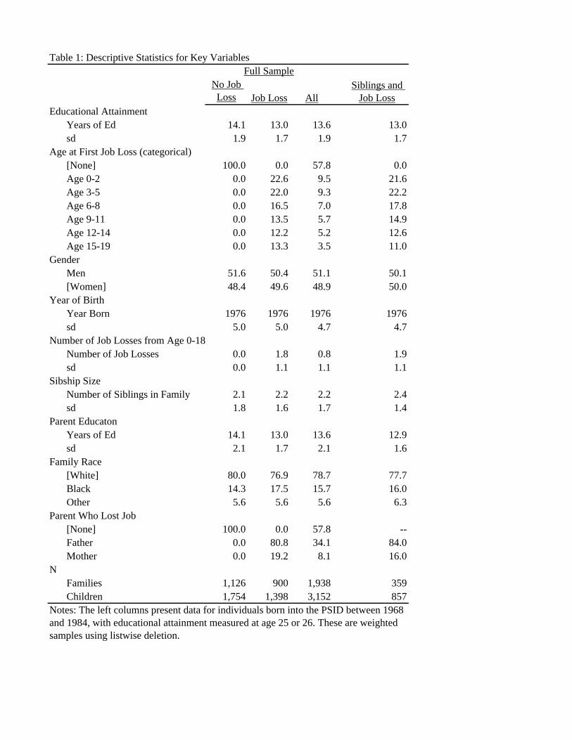
two or more siblings born between 1968 and 1984 experienced a head job loss. Table 1 contains

the descriptive statistics for both of these samples and is discussed below.

Measures

I use the terms “parental unemployment” or “parent job loss” to refer to any situation in

which a previously working parental head of household reports an involuntary end of employ-

ment. The PSID defines the “head” as the man in a two-parent household and only includes

women when there is no man to be the head of household. While far from ideal, the PSID did not

3 I have built a small correction into the weight to capture panel members who had data but do not have a

valid weight at age 25, generally due to re-entry into the survey. Only 179 of the 3150 members of my

sample had 0 or missing weights for the wave they turned 25. The 179 missing cases have weights taken

from the following wave, or the prior wave, depending on availability.

4 The results for a third sample, of individuals with siblings is presented in Appendix B, section four. The

results for this sample are similar to those presented in the core of the paper.


14

consistently collect data on “wives” employment status until 1979. The definition of unemploy-

ment encompasses two primary reasons for parental unemployment: layoff (generally due to eco-

nomic conditions, work place restructuring or business closure) or firing (when an employee is

let go due to job performance, behavioral issues or workplace politics).5Laid off or fired employ-

ees generally have no choice as to when and whether they exit the company, and have often little

warning.

There are three ways to operationalize parental unemployment: using the first spell of pa-

rental unemployment, creating a measure where children who experienced multiple job losses

were included in all of the groups, or using the longest parental unemployment spell as the refer-

ence. I choose to operationalize the timing of parental unemployment by focusing on the first

spell of unemployment for several reasons. Most importantly, that the results are substantively

similar to the measure including all of the parental job losses a child experiences, and the first

job loss measure has better model fit when measured by BIC’. (See Table 3 for the comparison

of the models. Results for the alternative measures of parental unemployment are in Appendix

B). Additionally, the first spell of unemployment serves as an important marker as it is the

child’s first exposure to the family level effects of unemployment, and prior research finds that

an unemployment spell increases the likelihood of unemployment in the short term (Fallick

1996; Stevens 1997). Using the first spell of parental unemployment fits well with cumulative

disadvantage theory since that theory is concerned with early life experiences. In order to prevent

age at the time of parental unemployment for potentially serving as a proxy for number of spells

5 Unfortunately, unless the firm closed, the PSID does not give detail about whether an individual was

part of a larger layoff or was fired.


15

experienced by the child, I control for the number of parental unemployment spells the child ex-

perienced from birth to age 19.

In this paper, I compare three separate strategies for measuring timing. In most life course

and developmental social-psychology research, the authors measures timing by dividing the ages

of children into 5 categories roughly corresponding to developmental stage. These categories are

young children (aged 0-5), older children (6-10), early adolescence (11-15), later adolescence

(16-18) and did not experience parental unemployment (for the models which include this group

it is the reference category) (e.g. Ermisch and Wright 1991; Ermisch, Francesconi and Pevalin

2004). These categories are potentially problematic as siblings aged 6 and 9 fall into the same

category, eliminating some variation within families. Table A1 presents the model fit for both of

these specifications along with continuous, cubic and quartic measures. To address this concern,

and because they were the best fitting models, I use a categorical variable with a three-year age

gradient instead, as the models have substantively similar results6.

I measure educational attainment as years of education completed. This continuous meas-

ure ranges from 11 (less than HS) to 17 (more than a BA, top coded by the PSID). Since siblings

tend to be more similar (even accounting for unobserved family characteristics) than a random

sample, measuring years of school completed will capture smaller differences in educational at-

tainment that would otherwise be lost using a categorical analysis. For example, two sisters who

both have attended “some college” have the same outcome in a categorical analysis, even though

the older sister persisted for 3 years before leaving and the younger sister left after her first year.

6 I include models using this specification in part 1 of Appendix B. The results do not differ substantially based on

how age is measured.


16

Children in smaller families tend to have higher levels of educational attainment (Felmlee

1988; Rich and Kim 1999), although the levels of educational attainment are more heterogeneous

in smaller families (Kuo and Hauser 1997). In the OLS regression portion of the paper, I include

number of siblings as a control for family size. While important to note, research on family size

does not provide any potential for predicting within family differences, only between family dif-

ferences7.

I also include a several controls. First, I control for gender in all of my models. This is

particularly important as sisters in this cohort have higher educational attainment than their

brothers do. In the OLS models, I also control for race, parent education (measured the same way

as the dependent variable), year of birth8, and female headed households at the time of the job

loss. There is no need to control for these variables in the fixed effects equations since they

measure family level characteristics.

Methods

I begin by presenting tables describing and figures illustrating the educational attainment

of children who experience parental unemployment compared to those who do not, with a focus

on age at the time of the job loss. Then I provide a base set of descriptive OLS regression anal-

yses with clustered standard errors to correct for siblings correlations. Finally, I use the sibling

7 I chose not to control for birth order because controlling for the oldest child may be over controlling as

many of the older children at the time of the first job loss may indeed by oldest children. However, when

the variable is included in the models the substantive results do not change.

8 Year of Birth is not multi-collinear with age at parental unemployment or birth order and the OLS re-

sults are similar with and without this variable.


17

data more fully by using family fixed effects models to estimate the impact of parental unem-

ployment timing on a child’s adult educational attainment. All models are weighted.

Family fixed effects models allow me to control for unmeasured family effects to better

tease out the specific effect of the age of the children at the time of parental unemployment

(Allison 2009; Conley, Pfeiffer and Velez 2007). The fixed effects model controls for (time in-

variant) family-specific contexts, such as the duration of the unemployment spell, parental stress,

financial strain, coping mechanisms and other unmeasured differences that vary between fami-

lies. A fixed effects model is analogous to an OLS regression but with dummy variables for each

family group (in this case with clustered standard errors, as discussed above)9.

Thus:

…

Where:

Y= Educational attainment in years at age 25;

= The age of the child the first time he or she experiences a parental job

loss;

… = The child level covariates for each child. The control variables are

gender, a dummy for oldest child in the family, year of birth, and number of job losses experi-

enced;

=The family level fixed effect which controls for differences

between families; and

9 For an in depth discussion of why I choose fixed effects models over random effects see Appendix B.


18

=The residual or error, which is assumed to be normally distributed and uncorrelated

with the family specific residual. This contains the variation caused by unobserved factors (any-

thing not in the model).

Fixed effects models control for time invariant family contexts. Fixed effects models do

not control for dynamic changes over time within families and thus do not perfectly control for

family context, specifically dynamic changes (such as marital dissolution) within families. How-

ever, they do provide the best available controls for family specific contexts, allowing me to fo-

cus on the child’s age at the time of job loss. Additionally, within-family differences remain, spe-

cifically children specific attributes such as intelligence, work ethic, personality etc.

RESULTS

TABLES 1 and 2 GO HERE

On average, individuals in the full sample attend school for thirteen and a half year before

age 25. The children who did not experience a parental head losing a job attended, on average,

14.1 years of school, approximately one year of schooling more than children who had a parent

lose his or her job at least once (with a mean of 13 years of school). Aside from that, the charac-

teristics of the children are similar, with slightly more than half of the respondents being young

women, one third are oldest siblings, and the mean year of birth is 1976. Forty-five percent of

children who experienced parental job loss did so before the age of six, with a mean age of

seven. In general the sample containing 857 siblings who had a parent lose his or her job (the

right column), is similar to the sample of 1398 children with parental job loss in the main sam-

ple. There are some differences between the children’s families. Children who have a parent lose


19

a job are slightly more likely to be black than white and to have parents with slightly lower edu-

cational attainment.

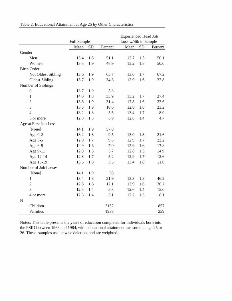
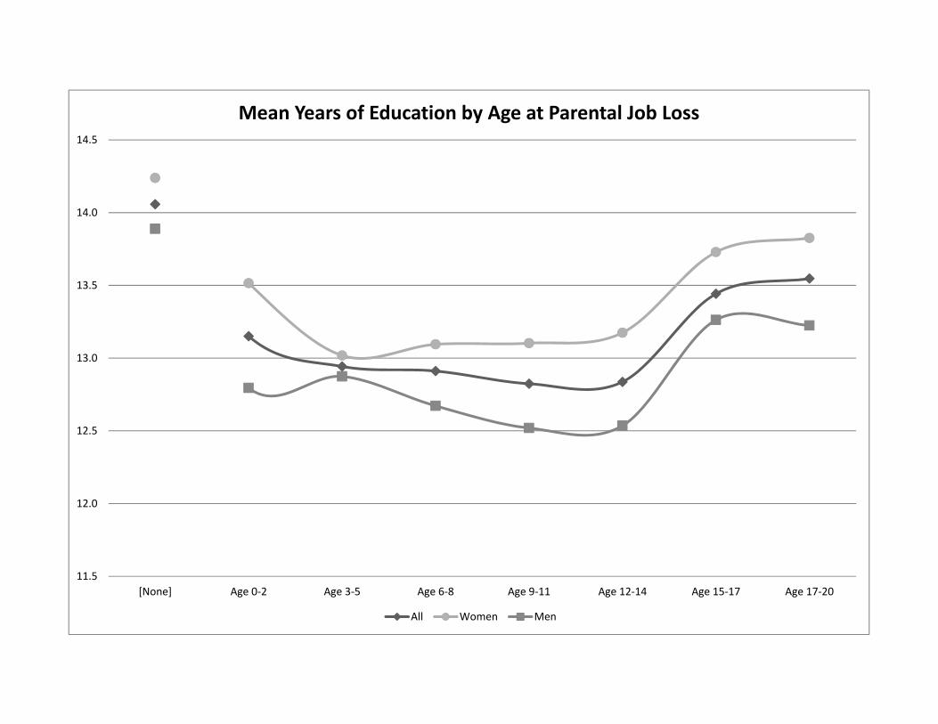
Table 2 focuses on the mean educational attainment for each of the groups described in

Table 1. (Figure 1 represents this graphically.) Descriptively, there is little difference in the edu-

cational attainment of children for children under the age of 15 at the time of the first parental

unemployment spell10. Importantly, there appears to be no relationship between age at time of

parent job loss and educational attainment. This suggests that there is likely no relationship be-

tween age at the time of parental unemployment and that if there is a relationship, it is non-lin-

ear. Cumulative disadvantage theory predicts either a linear relationship or between age at paren-

tal job loss and educational attainment since the relationship between age at first parental job loss

is not linear, this provides evidence that cumulative disadvantage theory likely does not explain

differences in educational attainment for children who experience parental unemployment.

The descriptive results indicate that age/life course stage may not be a major reason for

within-group difference in educational attainment and thus the family (fixed effects) results may

not support the hypotheses about age and life course effects of parental job loss on children. It is

important to continue examining the relationship between educational attainment and age at pa-

rental job loss because of the strong predictions of general life course theory.

10 An unweighted test of the mean differences (pwmean in stata) showed significant differences between

children who did not experience a parental unemployment spell and those who did experience a parental

unemployment spell. There was no significant difference in educational attainment for any group com-

pared to any other based on age at the time of first parental unemployment for children who experienced

parental unemployment. This test is only descriptive here since I used unweighted data.


20

TABLE 3 and FIGURE 1 about here

TABLE 4 GOES HERE

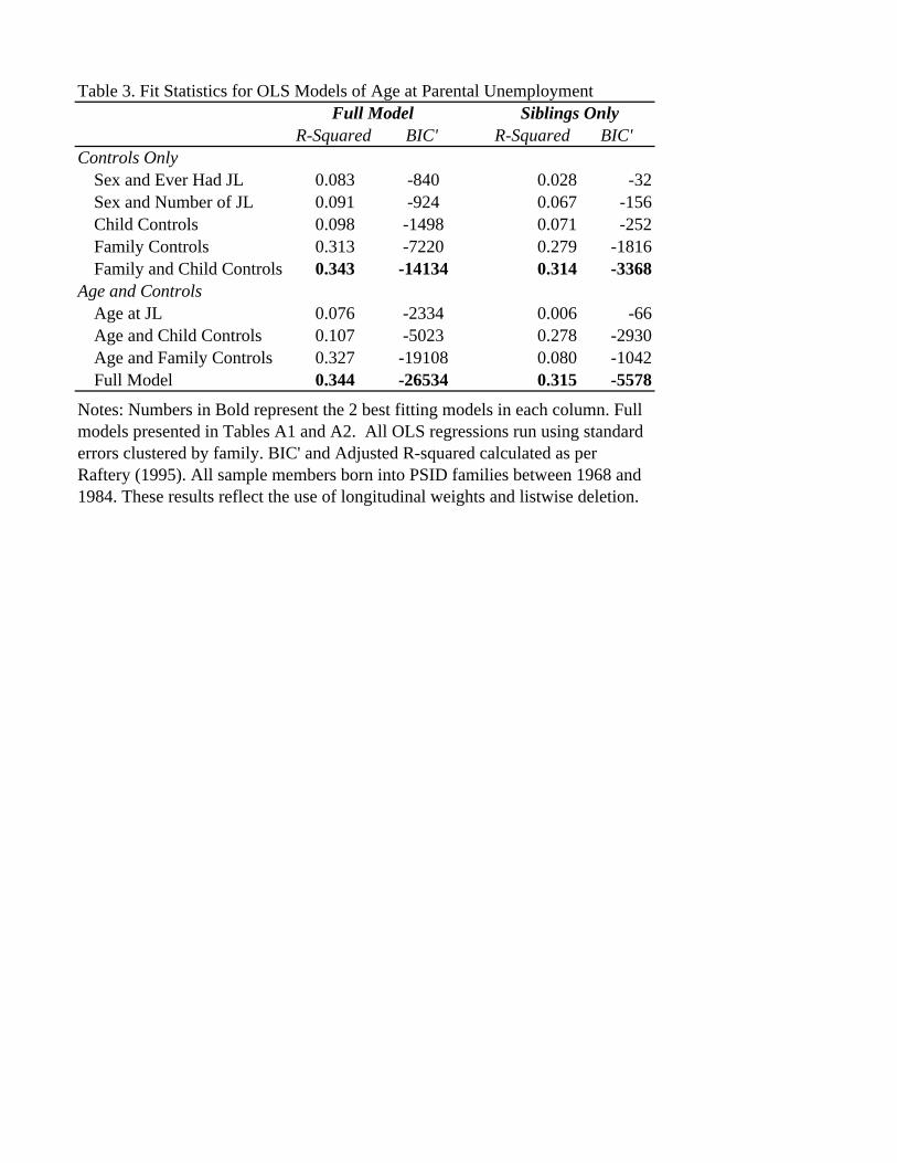
In table 3 I present the adjusted R2 and BIC’ for each OLS regression (Raftery 1995).

This allows me to compare model fit across models. Adding age increases the adjusted r-squared

values, (percentage of educational attainment explained) increases by .030 or .035, or 3 or 3.5

percentage points. The BIC’ measure of model fit suggests that age at the time of first parental

unemployment improves model fit for both the OLS and sibling fixed effects models compared

to models with only controls. The fit statistics suggest that including age at the time of first pa-

rental unemployment improves the overall model fit of educational attainment. In the next few

paragraphs, I examine the models in more detail.

TABLES 4 and 5 GO HERE

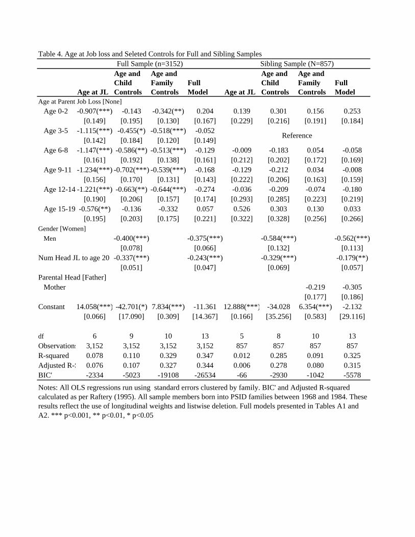
Table 4 includes the results of traditional OLS regressions of educational attainment re-

gressed on age at the time of parental job loss and controls for children’s and family characteris-

tics. The left columns in Table 4 compare child age at parental job loss to children whose parents

never experienced unemployment. Prior to adding controls, experiencing any parental job loss

predicts 1.2 years less educational attainment for children aged 9-11 and 12-14, compared with

children who do not experience job loss. In these full sample models (on the left) children who

did not experience a parental job loss are the reference category. Since prior research has shown


21

that parental unemployment is associated with lower educational attainment, in these full OLS

models it is not surprising that age at job loss is significant since the comparison group are chil-

dren with no parental job loss. After adding controls, age at any parental job loss shows smaller

differences in attainment. After controlling for child gender, age, year of birth, number of job

losses experienced11, parental education and family race the differences age at job loss is no

longer a significant predictor of educational attainment

The right columns of Table 4 present the educational attainment of children (with siblings

in the sample), who experienced parental unemployment. These models show that there is no sta-

tistically significant difference in educational attainment based on age at the time of parental un-

employment.

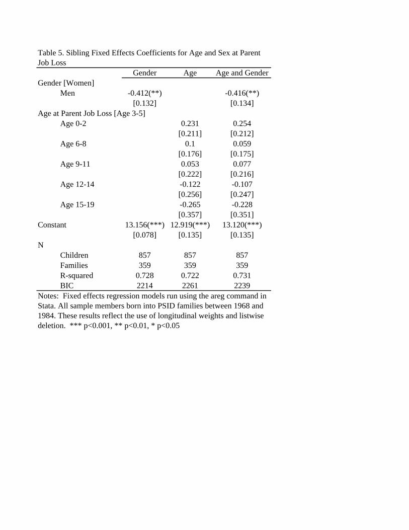
Table 5 provides the results of the fixed effects regression equations of age at the time of

job loss for children within families. Age at the time of parental unemployment generally does

not have a statistically significant effect on educational attainment in years for siblings12. Gender

is the only consistently significant predictor of educational attainment in the model, indicating

that on average sisters in the sample attended school for a .4 of a year more than their brothers.

11 The inclusion of number of job losses may cause concern about multicolinearity in my model. After ex-

amining the variable inflation factor (using estat vif in Stata), I find that this variable does not cause is-

sues in the model. Conceptually I include number of job losses as not to conflate age at the time of paren-

tal unemployment with experiencing parental unemployment at all.

12 These results are consistent using alternative measures of age at the time of parental unemployment.

See the appendices for more details.


22

The fixed effects findings are this consistent with the OLS findings that age at parental

unemployment is not a primary predictor of educational attainment. All of the models describe

about 73 percent of the within-family variation in educational attainment. Unfortunately, using

the PSID, I do not have access to individual level social-psychological characteristics, such as

ability or achievement (prior to job loss), motivation, or personality measures.

DISCUSSION

Life course and cumulative disadvantage theories strongly predict that the timing of pa-

rental unemployment in a child’s life should moderate children’s educational attainment. That is,

some of the within group difference in educational attainment for children who have a parent

lose his or her job is likely related to the development of the child, of which age is the primary

measure. Cumulative disadvantage specifies that younger children at the time of parental unem-

ployment experience more detrimental consequences in the long-term. Evidence for cumulative

disadvantage theory would come from a linear or non-linear relationship where younger children

at parental unemployment have lower educational attainment.

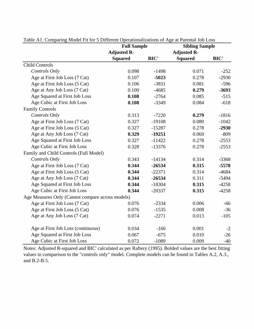
Counter to both life course and cumulative disadvantage theories, my findings suggest

that for children in families who have experienced a parent’s job loss, age at the time of the job

loss does not moderate their educational attainment compared to their siblings. Regardless how I

defined age at parental unemployment—using linear, four or 7 age categories, first or any job

loss (see appendices for details)—the models show little to no effect of age at parental unem-

ployment on siblings. The adjusted R-squared of the models, or the percent of variation de-

scribed by each model and “corrected” for the number of variables in the models—is generally

not higher for the age models than for models that only include the control variables. The “best”


23

model, the seven-category measure of age first parental unemployment spell improves model fit

by .004, or .4 percentage points, a very small amount.

In addition to the theoretical implications, my results are interesting for several reasons.

First the finding that age at parental unemployment is not significant indicates that either there

are few to no differences in the long term educational impacts of parental unemployment that

while the net association between age at parental unemployment and education is similar, but the

underlying processes differ. Future research may want to address the mechanisms by which pa-

rental unemployment harms educational attainment clarify if these mechanisms vary (by age).

Several less established perspectives are consistent with the possibility that the net associ-

ation between age at parental job loss and educational attainment is similar although the underly-

ing processes are likely different. Qualitative findings by Conley (2004) and Newman (1988)

suggest that older children at the time of job loss or other negative family changes experience

more of a negative impact because of their ability to take on more responsibility in the family.

When a parent loses his or her job, teenagers may be pressured to take on adult roles inside and

outside the home, and often voluntarily forgo higher education to enter the labor market to help

their families (Coelli 2011). Thus, the process of educational disadvantage for children who ex-

perience a parental job loss may be distinct by age, even if the long-term educational conse-

quences are the same.

My analyses are limited by a lack of information on children’s abilities, achievement, and

social-psychological characteristics prior to and post unemployment. This limitation means I

cannot control for individual differences between children, although that would likely not change

my results. The small sample size (857 children in 359 families, with half of them under 5 at the


24

time of the first job loss) may also be a reason why the models are not significant, but this does

not explain the low R-squared or model-fit values.

Other factors, aside from life course and age, may be useful in examining the association

between parent job loss and children’s lower educational attainment. One of these is similar to

research on poverty and educational attainment in that it addresses the duration and number of

unemployment spells. I will explore this further in future work. In future research I will examine

if family socioeconomic status prior to the unemployment spell focusing on family poverty status

and parent education moderate the impact of parental unemployment on children’s long-term ed-

ucational attainment.


25

APPENDIX A: FULL MODELS

Appendix A contains the full OLS models summarized in Table 3 and discussed in the

main body of the paper.


26

APPENDIX B: ALTERNATIVE MODEL SPECIFICATIONS/ROBUSTNESS

CHECKS

This appendix contains a series of alternative model specifications that serve as robust-

ness checks of the models in the main paper. None of these models changes the substantive re-

sults, although the point estimates are slightly different. Section 1 discusses four alternatives for

how to measure age at parental job loss and provides the results testing these models. The second

section presents random effects (RE) versions of the main models in the paper and explains why

fixed effects are more appropriate models for this paper. For each of these sections I provide a

short description of the robustness check, a series of tables presenting the results, and a very

short discussion of the results.

TABLE B.1 GOES HERE

Section 1: Alternative Age Measures

In the main paper, I operationalize age at parental job loss as a categorical measure of the

child’s age the first time a parental head of household loses his or her job. The first job loss

measure is a series of seven dummy variables measuring age at first job loss where each child is

counted once. Here I discuss three alternative ways to measure age at parental job loss: a 5-cate-

gory model of age at first job loss, age at any job loss, and continuous measures (Table B.1 pre-

sents the descriptive statistics). I discuss each of these in detail, then present the results (Tables

B.2-B.6) including comparing the model fit (Table B.2).

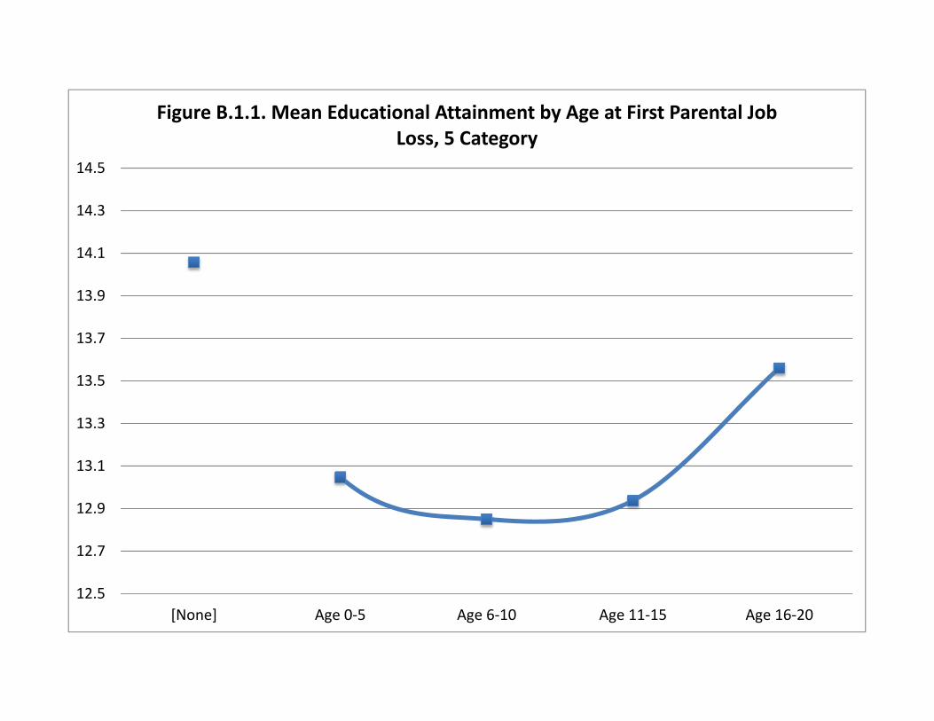
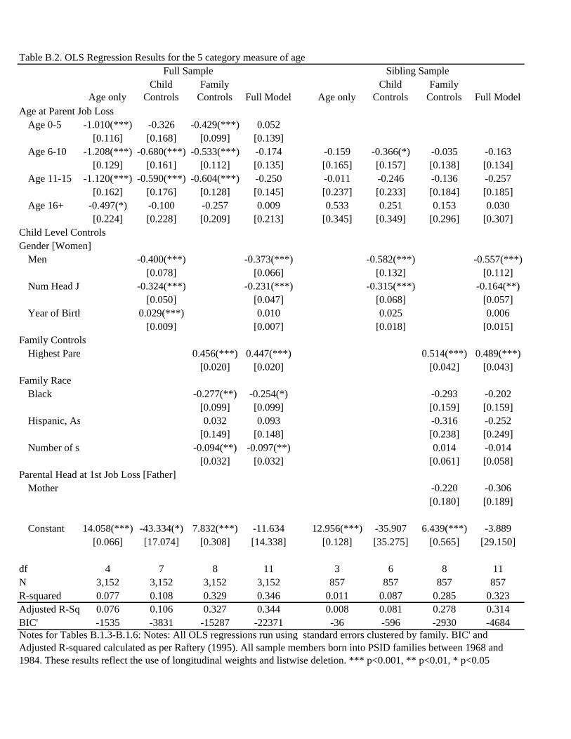
Age at first job loss: 5-category model

Prior life course and developmental social psychology research generally measures tim-

ing by dividing child ages into 5 categories roughly corresponding to developmental stage. These

categories are young children (aged 0-5), older children (6-10), early adolescence (11-15), and


27

later adolescence (16-19) (e.g. Ermisch and Wright 1991; Ermisch, Francesconi and Pevalin

2004). In this paper, these categories are potentially problematic as siblings aged 6 and 9 fall into

the same category, eliminating some variation within families. Figure B.1 and Table B.1. Present

the mean years of education for children using this measure and Table B.3. presents the OLS re-

gression results for these models.

FIGURE B.1 GOES HERE

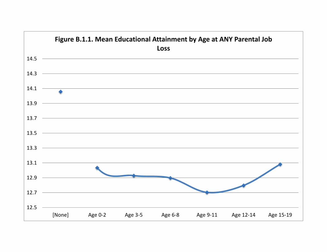
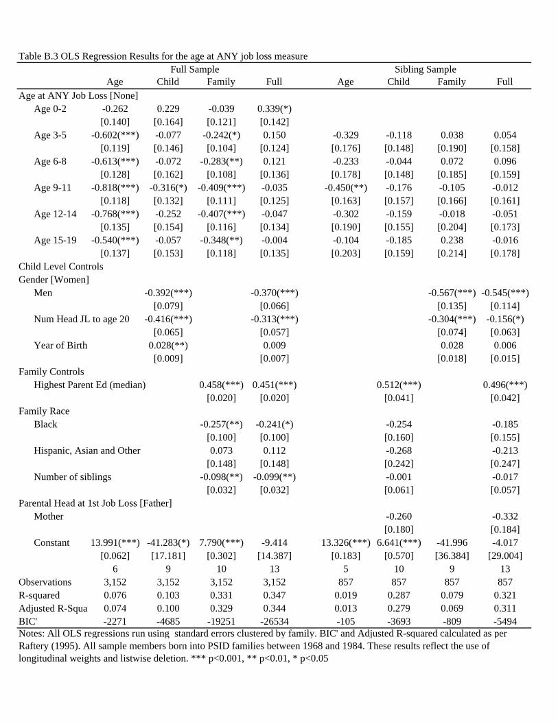
Age at any job loss

The cumulative measure summarizes at what age(s) a child experiences a parental job

loss considering all unemployment spells. For this measure, I use a series of dummy variables

where children are coded as 1 in ALL age categories in which they experienced parental unem-

ployment. This operationalization allows children with multiple exposures to job loss to be

counted as many times as they experienced a parent with a job loss. Table B. 4 presents the OLS

regression results for these models.

For example, two brothers Sam and Bill’s mother (the head of household) loses her job

twice, once when they boy are two and five and again when they are 10 and 13. When measuring

the first job loss, Sam is coded as a 1 in the 0-2 category and 0 for all other age categories. Like-

wise, Bill is coded 1 in the 3-5 age category and 0 in all of the others. Under the any job loss

measure, Sam is coded as a 1 in both the 0-2 and 9-11 categories and a 0 in the other categories.

Bill would be coded as a 1 in the 3-5 and 12-14 category. Thus, this measure captures all of the

age ranges when a child experiences a parental job loss. Figure B.2 and Table B.1 present the

mean years of education for children using this measure.



28

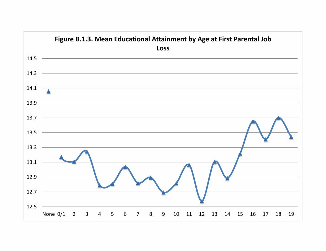
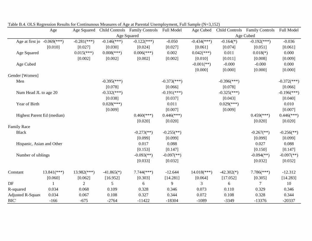
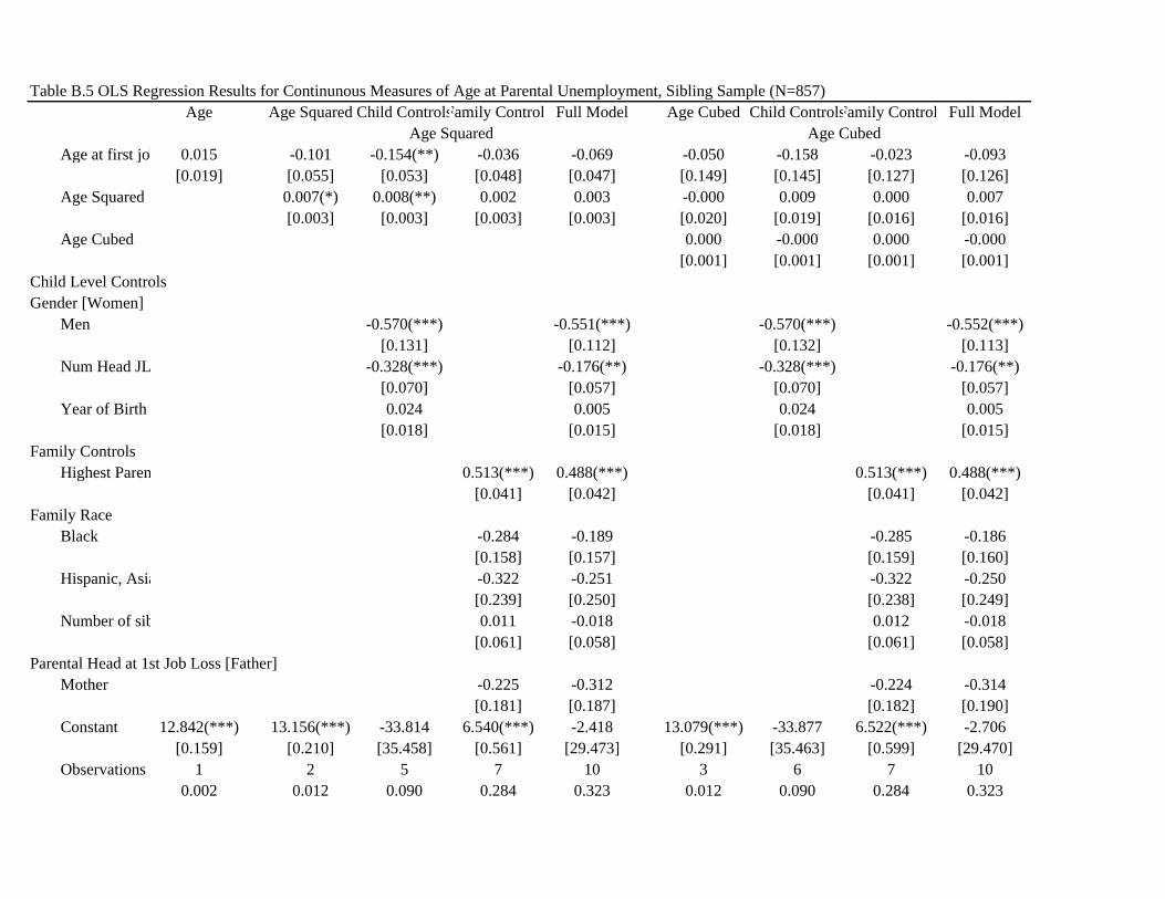
A continuous measure of age

Alternatively, utilizing age as a continuous variable, including a square and a cubic term,

allows for finer grained distinctions in the data while also allowing for non-linear relationships.

It is likely that the linear/square/and cubic terms may not capture the true shape of the distribu-

tion and thus not be very useful. Figure B.1.3 illustrates this challenge: there is no strong linear

trend.


Choosing a measure

Like figure 1 in the paper. Figures B.1 through B.3 show children’s mean educational at-

tainment by age at the time of the first parental job loss. Figure B.1, presents the mean educa-

tional attainment using a continuous measure (each age) of age at parental unemployment. The

trends displayed in the pattern are not statistically significant, nor are they linear for boys of

girls. Similar to Figure 1, Figure B.2 shows educational attainment by age category, also with no

trend.

TABLE B.2 GOES HERE

In the main body of the paper, I present a 7-category model of child age at first job loss.

In addition to the reasons listed in the main text, I chose to use first job loss because the results

are substantively similar and it is simpler to discuss the first job loss than any job loss. For the

final paper, I choose to use the seven-category model for three related reasons. First, they have

better model fit for the fully controlled OLS model based on BIC’ than the larger age ranges or a

continuous measure (see Table B.2). Second, the descriptive statistics indicate that this age at pa-

rental job loss is not a continuous predictor (see Figure B.1). The sample size is too small to in-

clude a dummy at each age, so I need to group the ages. While I need groupings, smaller age


29

ranges preserve a larger amount of the variation between children. By breaking age into 3 year

age groupings instead of 5 year groupings fewer siblings are likely to be in the same age cate-

gory at the time of the first parental job loss. Finally (and most importantly), as the models pre-

sented in Tables B.1.3-B.1.5 show, the substantive results are equivalent so the models are inter-

changeable.

TABLES B.1.3-B.1.5 GO HERE

Section 2: Random Effects Models

Over the course of this project, it has been suggested that random effects models may be

preferable to fixed effects models. While I conceptually prefer fixed effects models, I also show

results of random effects models and Hausman tests comparing the fixed and random effects

models. Consistent with prior robustness checks the results of random effects models are con-

sistent with the results from the models presented in the paper. More importantly, the Hausman

test indicates that the fixed effects model is mathematically more appropriate than the random

effects model

No Job Loss Job Loss All

Educational AttainmentYears of Ed 14.1 13.0 13.6 13.0sd 1.9 1.7 1.9 1.7

Age at First Job Loss (categorical)[None] 100.0 0.0 57.8 0.0Age 0-2 0.0 22.6 9.5 21.6Age 3-5 0.0 22.0 9.3 22.2Age 6-8 0.0 16.5 7.0 17.8Age 9-11 0.0 13.5 5.7 14.9Age 12-14 0.0 12.2 5.2 12.6Age 15-19 0.0 13.3 3.5 11.0

GenderMen 51.6 50.4 51.1 50.1[Women] 48.4 49.6 48.9 50.0

Year of BirthYear Born 1976 1976 1976 1976sd 5.0 5.0 4.7 4.7

Number of Job Losses from Age 0-18Number of Job Losses 0.0 1.8 0.8 1.9sd 0.0 1.1 1.1 1.1

Sibship SizeNumber of Siblings in Family 2.1 2.2 2.2 2.4sd 1.8 1.6 1.7 1.4

Parent EducatonYears of Ed 14.1 13.0 13.6 12.9sd 2.1 1.7 2.1 1.6

Family Race[White] 80.0 76.9 78.7 77.7Black 14.3 17.5 15.7 16.0Other 5.6 5.6 5.6 6.3

Parent Who Lost Job[None] 100.0 0.0 57.8 --Father 0.0 80.8 34.1 84.0Mother 0.0 19.2 8.1 16.0

NFamilies 1,126 900 1,938 359Children 1,754 1,398 3,152 857

Table 1: Descriptive Statistics for Key VariablesFull Sample

Notes: The left columns present data for individuals born into the PSID between 1968 and 1984, with educational attainment measured at age 25 or 26. These are weighted samples using listwise deletion.

Siblings and Job Loss

Mean SD Percent Mean SD PercentGender

Men 13.4 1.8 51.1 12.7 1.5 50.1Women 13.8 1.9 48.9 13.2 1.8 50.0

Birth OrderNot Oldest Sibling 13.6 1.9 65.7 13.0 1.7 67.2Oldest Sibling 13.7 1.9 34.3 12.9 1.6 32.8

Number of Siblings0 13.7 1.9 5.31 14.0 1.8 33.9 13.2 1.7 27.42 13.6 1.9 31.4 12.8 1.6 33.63 13.3 1.9 18.0 12.8 1.8 23.24 13.2 1.8 5.5 13.4 1.7 8.95 or more 12.8 1.5 5.9 12.8 1.4 4.7

Age at First Job Loss[None] 14.1 1.9 57.8Age 0-2 13.2 1.8 9.5 13.0 1.8 21.6Age 3-5 12.9 1.7 9.3 12.9 1.7 22.2Age 6-8 12.9 1.6 7.0 12.9 1.6 17.8Age 9-11 12.8 1.5 5.7 12.8 1.3 14.9Age 12-14 12.8 1.7 5.2 12.9 1.7 12.6Age 15-19 13.5 1.8 3.5 13.4 1.8 11.0

Number of Job Losses[None] 14.1 1.9 581 13.4 1.8 21.9 13.3 1.8 46.22 12.8 1.6 12.1 12.9 1.6 30.73 12.5 1.4 5.3 12.6 1.4 15.04 or more 12.3 1.4 3.1 12.2 1.3 8.1

N Children 3152 857Families 1938 359

Table 2: Educational Attainment at Age 25 by Other Characteristics

Full SampleExperienced Head Job Loss w/Sib in Sample

Notes: This table presents the years of education completed for individuals born into the PSID between 1968 and 1984, with educational attainment measured at age 25 or 26. These samples use listwise deletion, and are weighted.

11.5

12.0

12.5

13.0

13.5

14.0

14.5

[None] Age 0‐2 Age 3‐5 Age 6‐8 Age 9‐11 Age 12‐14 Age 15‐17 Age 17‐20

Mean Years of Education by Age at Parental Job Loss

All Women Men

R-Squared BIC' R-Squared BIC'Controls Only

Sex and Ever Had JL 0.083 -840 0.028 -32Sex and Number of JL 0.091 -924 0.067 -156Child Controls 0.098 -1498 0.071 -252Family Controls 0.313 -7220 0.279 -1816Family and Child Controls 0.343 -14134 0.314 -3368

Age and ControlsAge at JL 0.076 -2334 0.006 -66Age and Child Controls 0.107 -5023 0.278 -2930Age and Family Controls 0.327 -19108 0.080 -1042Full Model 0.344 -26534 0.315 -5578

Full Model Siblings OnlyTable 3. Fit Statistics for OLS Models of Age at Parental Unemployment

Notes: Numbers in Bold represent the 2 best fitting models in each column. Full models presented in Tables A1 and A2. All OLS regressions run using standard errors clustered by family. BIC' and Adjusted R-squared calculated as per Raftery (1995). All sample members born into PSID families between 1968 and 1984. These results reflect the use of longitudinal weights and listwise deletion.

Age at JL

Age and Child Controls

Age and Family Controls

Full Model Age at JL

Age and Child Controls

Age and Family Controls

Full Model

Age at Parent Job Loss [None]Age 0-2 -0.907(***) -0.143 -0.342(**) 0.204 0.139 0.301 0.156 0.253

[0.149] [0.195] [0.130] [0.167] [0.229] [0.216] [0.191] [0.184]Age 3-5 -1.115(***) -0.455(*) -0.518(***) -0.052

[0.142] [0.184] [0.120] [0.149]Age 6-8 -1.147(***) -0.586(**) -0.513(***) -0.129 -0.009 -0.183 0.054 -0.058

[0.161] [0.192] [0.138] [0.161] [0.212] [0.202] [0.172] [0.169]Age 9-11 -1.234(***) -0.702(***) -0.539(***) -0.168 -0.129 -0.212 0.034 -0.008

[0.156] [0.170] [0.131] [0.143] [0.222] [0.206] [0.163] [0.159]Age 12-14 -1.221(***) -0.663(**) -0.644(***) -0.274 -0.036 -0.209 -0.074 -0.180

[0.190] [0.206] [0.157] [0.174] [0.293] [0.285] [0.223] [0.219]Age 15-19 -0.576(**) -0.136 -0.332 0.057 0.526 0.303 0.130 0.033

[0.195] [0.203] [0.175] [0.221] [0.322] [0.328] [0.256] [0.266]Gender [Women]

Men -0.400(***) -0.375(***) -0.584(***) -0.562(***)[0.078] [0.066] [0.132] [0.113]

Num Head JL to age 20 -0.337(***) -0.243(***) -0.329(***) -0.179(**)[0.051] [0.047] [0.069] [0.057]

Parental Head [Father]Mother -0.219 -0.305

[0.177] [0.186]Constant 14.058(***) -42.701(*) 7.834(***) -11.361 12.888(***) -34.028 6.354(***) -2.132

[0.066] [17.090] [0.309] [14.367] [0.166] [35.256] [0.583] [29.116]

df 6 9 10 13 5 8 10 13Observations 3,152 3,152 3,152 3,152 857 857 857 857R-squared 0.078 0.110 0.329 0.347 0.012 0.285 0.091 0.325Adjusted R-S 0.076 0.107 0.327 0.344 0.006 0.278 0.080 0.315BIC' -2334 -5023 -19108 -26534 -66 -2930 -1042 -5578

Notes: All OLS regressions run using standard errors clustered by family. BIC' and Adjusted R-squared calculated as per Raftery (1995). All sample members born into PSID families between 1968 and 1984. These results reflect the use of longitudinal weights and listwise deletion. Full models presented in Tables A1 and A2. *** p<0.001, ** p<0.01, * p<0.05

Full Sample (n=3152) Sibling Sample (N=857)Table 4. Age at Job loss and Seleted Controls for Full and Sibling Samples

Reference

Gender Age Age and GenderGender [Women]

Men -0.412(**) -0.416(**)[0.132] [0.134]

Age at Parent Job Loss [Age 3-5]Age 0-2 0.231 0.254

[0.211] [0.212]Age 6-8 0.1 0.059

[0.176] [0.175]Age 9-11 0.053 0.077

[0.222] [0.216]Age 12-14 -0.122 -0.107

[0.256] [0.247]Age 15-19 -0.265 -0.228

[0.357] [0.351]Constant 13.156(***) 12.919(***) 13.120(***)

[0.078] [0.135] [0.135]N

Children 857 857 857Families 359 359 359R-squared 0.728 0.722 0.731BIC 2214 2261 2239

Table 5. Sibling Fixed Effects Coefficients for Age and Sex at Parent Job Loss

Notes: Fixed effects regression models run using the areg command in Stata. All sample members born into PSID families between 1968 and 1984. These results reflect the use of longitudinal weights and listwise deletion. *** p<0.001, ** p<0.01, * p<0.05

Adjusted R-Squared BIC'

Adjusted R-Squared BIC'

Child ControlsControls Only 0.098 -1498 0.071 -252Age at First Job Loss (7 Cat) 0.107 -5023 0.278 -2930Age at First Job Loss (5 Cat) 0.106 -3831 0.081 -596Age at Any Job Loss (7 Cat) 0.100 -4685 0.279 -3693Age Squared at First Job Loss 0.108 -2764 0.085 -515Age Cubic at First Job Loss 0.108 -3349 0.084 -618

Family ControlsControls Only 0.313 -7220 0.279 -1816Age at First Job Loss (7 Cat) 0.327 -19108 0.080 -1042Age at First Job Loss (5 Cat) 0.327 -15287 0.278 -2930Age at Any Job Loss (7 Cat) 0.329 -19251 0.069 -809Age Squared at First Job Loss 0.327 -11422 0.278 -2553Age Cubic at First Job Loss 0.328 -13376 0.278 -2553

Family and Child Controls (Full Model)Controls Only 0.343 -14134 0.314 -3368Age at First Job Loss (7 Cat) 0.344 -26534 0.315 -5578Age at First Job Loss (5 Cat) 0.344 -22371 0.314 -4684Age at Any Job Loss (7 Cat) 0.344 -26534 0.311 -5494Age Squared at First Job Loss 0.344 -18304 0.315 -4258Age Cubic at First Job Loss 0.344 -20337 0.315 -4258

Age Measures Only (Cannot compare across models)Age at First Job Loss (7 Cat) 0.076 -2334 0.006 -66Age at First Job Loss (5 Cat) 0.076 -1535 0.008 -36Age at Any Job Loss (7 Cat) 0.074 -2271 0.013 -105

Age at First Job Loss (continuous) 0.034 -166 0.001 -2Age Squared at First Job Loss 0.067 -675 0.010 -26Age Cubic at First Job Loss 0.072 -1089 0.009 -40

Full Sample Sibling SampleTable A1. Comparing Model Fit for 5 Different Operationalizations of Age at Parental Job Loss

Notes: Adjusted R-squared and BIC' calculated as per Raftery (1995). Bolded values are the best fitting values in comparison to the "controls only" model. Complete models can be found in Tables A.2, A.3., and B.2-B.5.

Base Model

Gender & Num JL Child Family Family &

Child Age at JL Age & Child

Age & Family

Full Model

Age at Parent Job Loss [None]Age 0-2 -0.907(***) -0.143 -0.342(**) 0.204

[0.149] [0.195] [0.130] [0.167]Age 3-5 -1.115(***) -0.455(*) -0.518(***) -0.052

[0.142] [0.184] [0.120] [0.149]Age 6-8 -1.147(***) -0.586(**) -0.513(***) -0.129

[0.161] [0.192] [0.138] [0.161]Age 9-11 -1.234(***) -0.702(***) -0.539(***) -0.168

[0.156] [0.170] [0.131] [0.143]Age 12-14 -1.221(***) -0.663(**) -0.644(***) -0.274

[0.190] [0.206] [0.157] [0.174]Age 15-19 -0.576(**) -0.136 -0.332 0.057

[0.195] [0.203] [0.175] [0.221]Child Level ControlsParent Job Loss [No Job Loss]

Job Loss -1.036(***)[0.095]

Num Head JL to age 20 -0.475(***) -0.472(***) -0.243(***) -0.337(***) -0.243(***)[0.035] [0.035] [0.032] [0.051] [0.047]

Gender [Women]Men -0.401(***) -0.389(***) -0.388(***) -0.371(***) -0.400(***) -0.375(***)

[0.079] [0.079] [0.079] [0.067] [0.078] [0.066]Year of Birth 0.030(***) 0.011 0.029(***) 0.010

[0.009] [0.007] [0.009] [0.007]Family Level Controls

Highest Parent Ed (median) 0.490(***) 0.451(***) 0.456(***) 0.448(***)[0.020] [0.020] [0.020] [0.020]

Family Race [White]Black/African American -0.258(*) -0.247(*) -0.273(**) -0.246(*)

[0.104] [0.100] [0.099] [0.099]Hispanic, Asian, and Other 0.066 0.124 0.033 0.099

[0.160] [0.146] [0.149] [0.148]Number of siblings -0.099(**) -0.100(**) -0.095(**) -0.098(**)

[0.033] [0.032] [0.032] [0.032]Constant 14.265(***)14.183(***)-44.467(**) 7.177(***) -14.147 14.058(***) -42.701(*) 7.834(***) -11.361

[0.077] [0.072] [17.075] [0.290] [14.194] [0.066] [17.090] [0.309] [14.367]

df 2 2 3 4 7 6 9 10 13Observations 3,152 3,152 3,152 3,152 3,152 3,152 3,152 3,152 3,152R-squared 0.084 0.092 0.099 0.314 0.344 0.078 0.110 0.329 0.347Adjusted R-Sq 0.083 0.091 0.098 0.313 0.343 0.076 0.107 0.327 0.344BIC' -840 -924 -1498 -7220 -14134 -2334 -5023 -19108 -26534BIC' Compared to Control -84 -573 -12636 -2689 -16775 -24200Model compared 1 2 3 6 6 6

Table A2: Full Models for the Full Sample (Table 4)

Notes: All OLS regressions run using standard errors clustered by family. BIC' and Adjusted R-squared calculated as per Raftery (1995). All sample members born into PSID families between 1968 and 1984. These results reflect the use of longitudinal weights and listwise deletion. *** p<0.001, ** p<0.01, * p<0.05

Gender Gender & Num JL Child Family Family &

Child Age at JL Age & Child

Age & Family Full Model

Age at Parent Job Loss [Age 3-5]

Age 0-2 0.139 0.301 0.156 0.253[0.229] [0.216] [0.191] [0.184]

Age 6-8 -0.009 -0.183 0.054 -0.058[0.212] [0.202] [0.172] [0.169]

Age 9-11 -0.129 -0.212 0.034 -0.008[0.222] [0.206] [0.163] [0.159]

Age 12-14 -0.036 -0.209 -0.074 -0.180[0.293] [0.285] [0.223] [0.219]

Age 15-19 0.526 0.303 0.130 0.033[0.322] [0.328] [0.256] [0.266]

Child Level ControlsNum Head JL to age 20 -0.306(***) -0.299(***) -0.143(*) -0.329(***) -0.179(**)

[0.064] [0.065] [0.056] [0.069] [0.057]Gender [Women

Male -0.573(***) -0.537(***) -0.555(***) -0.549(***) -0.584(***) -0.562(***)[0.133] [0.133] [0.134] [0.113] [0.132] [0.113]

Year of Birth 0.025 0.008 0.024 0.005[0.018] [0.014] [0.018] [0.015]

Family Level Controls

Highest Parent 0.516(***) 0.494(***) 0.514(***) 0.489(***)[0.042] [0.043] [0.041] [0.042]

Family Race [White]Black/Afric -0.281 -0.183 -0.289 -0.195

[0.155] [0.154] [0.156] [0.157]Hispanic, A -0.299 -0.211 -0.309 -0.236

[0.227] [0.237] [0.241] [0.252]Number of sibli 0.011 -0.015 0.013 -0.018

[0.060] [0.057] [0.061] [0.059]Which Parent is Head [Father]

Mother -0.240 -0.342 -0.219 -0.305[0.177] [0.183] [0.177] [0.186]

Constant 13.237(***) 13.798(***) -36.309 6.391(***) -9.274 12.888(***) -34.028 6.354(***) -2.132[0.126] [0.194] [36.125] [0.553] [28.314] [0.166] [35.256] [0.583] [29.116]

df 1 2 3 5 8 5 8 10 13Observations 857 857 857 857 857 857 857 857 857R-squared 0.029 0.069 0.074 0.283 0.320 0.012 0.285 0.091 0.325Adjusted R-Sq 0.028 0.067 0.071 0.279 0.314 0.006 0.278 0.080 0.315BIC' -32 -156 -252 -1816 -3368 -66 -2930 -1042 -5578BIC' Compared to Controls -124 -96 -1552 -2864 -976 -5512Model compared 1 2 3 6 6 6

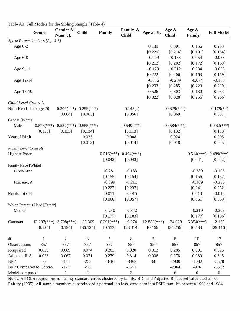
Table A3: Full Models for the Sibling Sample (Table 4)

Notes: All OLS regressions run using standard errors clustered by family. BIC' and Adjusted R-squared calculated as per Raftery (1995). All sample members expereineced a parental job loss, were born into PSID families between 1968 and 1984

with at least one sibling born durring those years . These results reflect the use of longitudinal weights and listwise deletion. *** p<0.001, ** p<0.01, * p<0.05

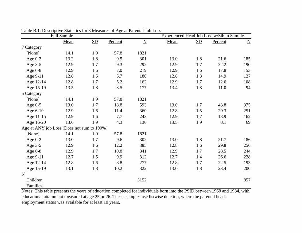
Mean SD Percent N Mean SD Percent N7 Category

[None] 14.1 1.9 57.8 1821Age 0-2 13.2 1.8 9.5 301 13.0 1.8 21.6 185Age 3-5 12.9 1.7 9.3 292 12.9 1.7 22.2 190Age 6-8 12.9 1.6 7.0 219 12.9 1.6 17.8 153Age 9-11 12.8 1.5 5.7 180 12.8 1.3 14.9 127Age 12-14 12.8 1.7 5.2 162 12.9 1.7 12.6 108Age 15-19 13.5 1.8 3.5 177 13.4 1.8 11.0 94

5 Category[None] 14.1 1.9 57.8 1821Age 0-5 13.0 1.7 18.8 593 13.0 1.7 43.8 375Age 6-10 12.9 1.6 11.4 360 12.8 1.5 29.3 251Age 11-15 12.9 1.6 7.7 243 12.9 1.7 18.9 162Age 16-20 13.6 1.9 4.3 136 13.5 1.9 8.1 69

Age at ANY job Loss (Does not sum to 100%)[None] 14.1 1.9 57.8 1821Age 0-2 13.0 1.7 9.6 302 13.0 1.8 21.7 186Age 3-5 12.9 1.6 12.2 385 12.8 1.6 29.8 256Age 6-8 12.9 1.7 10.8 341 12.9 1.7 28.5 244Age 9-11 12.7 1.5 9.9 312 12.7 1.4 26.6 228Age 12-14 12.8 1.6 8.8 277 12.8 1.7 22.5 193Age 15-19 13.1 1.8 10.2 322 13.0 1.8 23.4 200

N Children 3152 857Families

Full Sample Experienced Head Job Loss w/Sib in SampleTable B.1: Descriptive Statistics for 3 Measures of Age at Parental Job Loss

Notes: This table presents the years of education completed for individuals born into the PSID between 1968 and 1984, with educational attainment measured at age 25 or 26. These samples use listwise deletion, where the parental head's employment status was available for at least 10 years.

12.5

12.7

12.9

13.1

13.3

13.5

13.7

13.9

14.1

14.3

14.5

[None] Age 0‐5 Age 6‐10 Age 11‐15 Age 16‐20

Figure B.1.1. Mean Educational Attainment by Age at First Parental Job Loss, 5 Category

12.5

12.7

12.9

13.1

13.3

13.5

13.7

13.9

14.1

14.3

14.5

[None] Age 0‐2 Age 3‐5 Age 6‐8 Age 9‐11 Age 12‐14 Age 15‐19

Figure B.1.1. Mean Educational Attainment by Age at ANY Parental Job Loss

12.5

12.7

12.9

13.1

13.3

13.5

13.7

13.9

14.1

14.3

14.5

None 0/1 2 3 4 5 6 7 8 9 10 11 12 13 14 15 16 17 18 19

Figure B.1.3. Mean Educational Attainment by Age at First Parental Job Loss

Age onlyChild

ControlsFamily

Controls Full Model Age onlyChild

ControlsFamily

Controls Full ModelAge at Parent Job Loss

Age 0-5 -1.010(***) -0.326 -0.429(***) 0.052[0.116] [0.168] [0.099] [0.139]

Age 6-10 -1.208(***) -0.680(***) -0.533(***) -0.174 -0.159 -0.366(*) -0.035 -0.163[0.129] [0.161] [0.112] [0.135] [0.165] [0.157] [0.138] [0.134]

Age 11-15 -1.120(***) -0.590(***) -0.604(***) -0.250 -0.011 -0.246 -0.136 -0.257[0.162] [0.176] [0.128] [0.145] [0.237] [0.233] [0.184] [0.185]

Age 16+ -0.497(*) -0.100 -0.257 0.009 0.533 0.251 0.153 0.030[0.224] [0.228] [0.209] [0.213] [0.345] [0.349] [0.296] [0.307]

Child Level ControlsGender [Women]

Men -0.400(***) -0.373(***) -0.582(***) -0.557(***)[0.078] [0.066] [0.132] [0.112]

Num Head JL -0.324(***) -0.231(***) -0.315(***) -0.164(**)[0.050] [0.047] [0.068] [0.057]

Year of Birth 0.029(***) 0.010 0.025 0.006[0.009] [0.007] [0.018] [0.015]

Family ControlsHighest Pare 0.456(***) 0.447(***) 0.514(***) 0.489(***)

[0.020] [0.020] [0.042] [0.043]Family Race

Black -0.277(**) -0.254(*) -0.293 -0.202[0.099] [0.099] [0.159] [0.159]

Hispanic, As 0.032 0.093 -0.316 -0.252[0.149] [0.148] [0.238] [0.249]

Number of si -0.094(**) -0.097(**) 0.014 -0.014[0.032] [0.032] [0.061] [0.058]

Parental Head at 1st Job Loss [Father]Mother -0.220 -0.306

[0.180] [0.189]

Constant 14.058(***) -43.334(*) 7.832(***) -11.634 12.956(***) -35.907 6.439(***) -3.889[0.066] [17.074] [0.308] [14.338] [0.128] [35.275] [0.565] [29.150]

df 4 7 8 11 3 6 8 11N 3,152 3,152 3,152 3,152 857 857 857 857R-squared 0.077 0.108 0.329 0.346 0.011 0.087 0.285 0.323Adjusted R-Squ 0.076 0.106 0.327 0.344 0.008 0.081 0.278 0.314BIC' -1535 -3831 -15287 -22371 -36 -596 -2930 -4684

Table B.2. OLS Regression Results for the 5 category measure of ageFull Sample Sibling Sample

Notes for Tables B.1.3-B.1.6: Notes: All OLS regressions run using standard errors clustered by family. BIC' and Adjusted R-squared calculated as per Raftery (1995). All sample members born into PSID families between 1968 and 1984. These results reflect the use of longitudinal weights and listwise deletion. *** p<0.001, ** p<0.01, * p<0.05

Age Child Family Full Age Child Family FullAge at ANY Job Loss [None]

Age 0-2 -0.262 0.229 -0.039 0.339(*)[0.140] [0.164] [0.121] [0.142]

Age 3-5 -0.602(***) -0.077 -0.242(*) 0.150 -0.329 -0.118 0.038 0.054[0.119] [0.146] [0.104] [0.124] [0.176] [0.148] [0.190] [0.158]

Age 6-8 -0.613(***) -0.072 -0.283(**) 0.121 -0.233 -0.044 0.072 0.096[0.128] [0.162] [0.108] [0.136] [0.178] [0.148] [0.185] [0.159]

Age 9-11 -0.818(***) -0.316(*) -0.409(***) -0.035 -0.450(**) -0.176 -0.105 -0.012[0.118] [0.132] [0.111] [0.125] [0.163] [0.157] [0.166] [0.161]

Age 12-14 -0.768(***) -0.252 -0.407(***) -0.047 -0.302 -0.159 -0.018 -0.051[0.135] [0.154] [0.116] [0.134] [0.190] [0.155] [0.204] [0.173]

Age 15-19 -0.540(***) -0.057 -0.348(**) -0.004 -0.104 -0.185 0.238 -0.016[0.137] [0.153] [0.118] [0.135] [0.203] [0.159] [0.214] [0.178]


Men -0.392(***) -0.370(***) -0.567(***) -0.545(***)[0.079] [0.066] [0.135] [0.114]

Num Head JL to age 20 -0.416(***) -0.313(***) -0.304(***) -0.156(*)[0.065] [0.057] [0.074] [0.063]

Year of Birth 0.028(**) 0.009 0.028 0.006[0.009] [0.007] [0.018] [0.015]

Family ControlsHighest Parent Ed (median) 0.458(***) 0.451(***) 0.512(***) 0.496(***)

[0.020] [0.020] [0.041] [0.042]Family Race

Black -0.257(**) -0.241(*) -0.254 -0.185[0.100] [0.100] [0.160] [0.155]

Hispanic, Asian and Other 0.073 0.112 -0.268 -0.213[0.148] [0.148] [0.242] [0.247]

Number of siblings -0.098(**) -0.099(**) -0.001 -0.017[0.032] [0.032] [0.061] [0.057]

Parental Head at 1st Job Loss [Father]Mother -0.260 -0.332

[0.180] [0.184]Constant 13.991(***) -41.283(*) 7.790(***) -9.414 13.326(***) 6.641(***) -41.996 -4.017

[0.062] [17.181] [0.302] [14.387] [0.183] [0.570] [36.384] [29.004]6 9 10 13 5 10 9 13

Observations 3,152 3,152 3,152 3,152 857 857 857 857R-squared 0.076 0.103 0.331 0.347 0.019 0.287 0.079 0.321Adjusted R-Squar 0.074 0.100 0.329 0.344 0.013 0.279 0.069 0.311BIC' -2271 -4685 -19251 -26534 -105 -3693 -809 -5494

Table B.3 OLS Regression Results for the age at ANY job loss measureFull Sample Sibling Sample


Age Age Squared Child Controls Family Controls Full Model Age Cubed Child Controls Family Controls Full Model

Age at first job -0.069(***) -0.281(***) -0.146(***) -0.122(***) -0.050 -0.434(***) -0.164(*) -0.192(***) -0.036[0.010] [0.027] [0.030] [0.024] [0.027] [0.061] [0.074] [0.051] [0.061]

Age Squared 0.015(***) 0.008(***) 0.006(***) 0.002 0.042(***) 0.011 0.018(*) 0.000[0.002] [0.002] [0.002] [0.002] [0.010] [0.011] [0.008] [0.009]

Age Cubed -0.001(**) -0.000 -0.000 0.000[0.000] [0.000] [0.000] [0.000]

Gender [Women]Men -0.395(***) -0.373(***) -0.396(***) -0.372(***)

[0.078] [0.066] [0.078] [0.066]Num Head JL to age 20 -0.332(***) -0.191(***) -0.325(***) -0.196(***)

[0.038] [0.037] [0.043] [0.040]Year of Birth 0.028(***) 0.011 0.029(***) 0.010

[0.009] [0.007] [0.009] [0.007]Highest Parent Ed (median) 0.460(***) 0.446(***) 0.459(***) 0.446(***)

[0.020] [0.020] [0.020] [0.020]Family Race

Black -0.273(**) -0.255(**) -0.267(**) -0.256(**)[0.099] [0.099] [0.099] [0.099]

Hispanic, Asian and Other 0.017 0.088 0.027 0.088[0.153] [0.147] [0.150] [0.147]

Number of siblings -0.093(**) -0.097(**) -0.094(**) -0.097(**)[0.033] [0.032] [0.032] [0.032]

Constant 13.841(***) 13.982(***) -41.865(*) 7.744(***) -12.644 14.018(***) -42.302(*) 7.786(***) -12.312[0.060] [0.062] [16.952] [0.303] [14.281] [0.064] [17.052] [0.305] [14.283]

DF 1 2 5 6 9 3 6 7 10R-squared 0.034 0.068 0.109 0.328 0.346 0.073 0.110 0.329 0.346Adjusted R-Square 0.034 0.067 0.108 0.327 0.344 0.072 0.108 0.328 0.344BIC' -166 -675 -2764 -11422 -18304 -1089 -3349 -13376 -20337

Table B.4. OLS Regression Results for Continunous Measures of Age at Parental Unemployment, Full Sample (N=3,152)

Age Squared Age Cubed


Age Age Squared Child ControlsFamily Control Full Model Age Cubed Child ControlsFamily Control Full Model

Age at first job 0.015 -0.101 -0.154(**) -0.036 -0.069 -0.050 -0.158 -0.023 -0.093[0.019] [0.055] [0.053] [0.048] [0.047] [0.149] [0.145] [0.127] [0.126]

Age Squared 0.007(*) 0.008(**) 0.002 0.003 -0.000 0.009 0.000 0.007[0.003] [0.003] [0.003] [0.003] [0.020] [0.019] [0.016] [0.016]

Age Cubed 0.000 -0.000 0.000 -0.000[0.001] [0.001] [0.001] [0.001]


Men -0.570(***) -0.551(***) -0.570(***) -0.552(***)[0.131] [0.112] [0.132] [0.113]

Num Head JL -0.328(***) -0.176(**) -0.328(***) -0.176(**)[0.070] [0.057] [0.070] [0.057]

Year of Birth 0.024 0.005 0.024 0.005[0.018] [0.015] [0.018] [0.015]

Family ControlsHighest Paren 0.513(***) 0.488(***) 0.513(***) 0.488(***)

[0.041] [0.042] [0.041] [0.042]Family Race

Black -0.284 -0.189 -0.285 -0.186[0.158] [0.157] [0.159] [0.160]

Hispanic, Asia -0.322 -0.251 -0.322 -0.250[0.239] [0.250] [0.238] [0.249]

Number of sib 0.011 -0.018 0.012 -0.018[0.061] [0.058] [0.061] [0.058]

Parental Head at 1st Job Loss [Father]Mother -0.225 -0.312 -0.224 -0.314

[0.181] [0.187] [0.182] [0.190]Constant 12.842(***) 13.156(***) -33.814 6.540(***) -2.418 13.079(***) -33.877 6.522(***) -2.706

[0.159] [0.210] [35.458] [0.561] [29.473] [0.291] [35.463] [0.599] [29.470]Observations 1 2 5 7 10 3 6 7 10

0.002 0.012 0.090 0.284 0.323 0.012 0.090 0.284 0.323

Table B.5 OLS Regression Results for Continunous Measures of Age at Parental Unemployment, Sibling Sample (N=857)

Age Squared Age Cubed

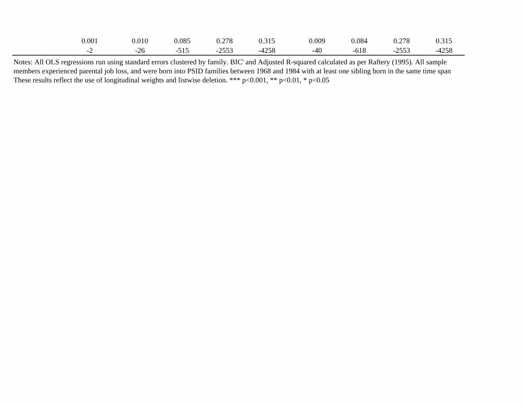
0.001 0.010 0.085 0.278 0.315 0.009 0.084 0.278 0.315-2 -26 -515 -2553 -4258 -40 -618 -2553 -4258

Notes: All OLS regressions run using standard errors clustered by family. BIC' and Adjusted R-squared calculated as per Raftery (1995). All sample members experienced parental job loss, and were born into PSID families between 1968 and 1984 with at least one sibling born in the same time span These results reflect the use of longitudinal weights and listwise deletion. *** p<0.001, ** p<0.01, * p<0.05


51

WORKS CITED

2013. "Panel Study of Income Dynamics, public use dataset." edited by Institute for Social Research Survey Research Center. Ann Arbor, MI: University of Michigan.

Allison, Paul D. 2009. Fixed Effects Regression Models. Thousand Oaks, CA: Sage. Almond, Douglas, and Janet Currie. 2011. "Human Capital Development before Age Five." Pp. 1315-486 in Handbook of Labor

Economics, edited by Ashenfelter Orley and Card David: Elsevier. Ananat, Elizabeth O., Anna Gassman-Pines, and Christina M. Gibson-Davis. 2011. "The Effects of Local Employment Losses on

Children’s Educational Achievement." Pp. 299-314 in Whither Opportunity? Rising Inequality, Schools, and Children's Life Chances, edited by Greg J. Duncan and Richard J. Murnane. New York: Russel Sage.

Andersen, Signe Hald. 2013. "Common Genes or Exogenous Shock? Disentangling the Causal Effect of Paternal Unemployment on Children's Schooling Efforts." European Sociological Review 29(3):477-88.

Brand, Jennie E., and Juli Simon Thomas. Forthcoming. "Job Displacement Among Single Mothers: Effects On Children's Outcomes in Young Adulthood." American Journal of Sociology xx(xx):xx.

Bratberg, Espen, Øivind Anti Nilsen, and Kjell Vaage. 2008. "Job losses and child outcomes." Labour Economics 15(4):591-603. Coelli, Michael B. 2011. "Parental job loss and the education enrollment of youth." Labour Economics 18(1):25-35. Conley, Dalton. 2004. The Pecking Order: Which Siblings Succeed and Why: Pantheon. Conley, Dalton, and Rebecca Glauber. 2008. "All in the family?: Family composition, resources, and sibling similarity in

socioeconomic status." Research in Social Stratification and Mobility 26(4):297-306. Conley, Dalton, Kathryn M. Pfeiffer, and Melissa Velez. 2007. "Explaining sibling differences in achievement and behavioral

outcomes: The importance of within- and between-family factors." Social Science Research 36(3):1087-104. Cunha, Flavio, and James J. Heckman. 2010. "Investing in Our Young People." National Bureau of Economic Research Working

Paper Series No. 16201. Dannefer, Dale. 2003. "Cumulative Advantage/Disadvantage and the Life Course: Cross-Fertilizing Age and Social Science

Theory." The Journals of Gerontology Series B: Psychological Sciences and Social Sciences 58(6):S327-S37. DiPrete, Thomas A., and Gregory M. Eirich. 2006. "Cumulative Advantage As a Mechanism for Inequality: A Review of

Theoretical and Empirical Developments." Annual Review of Sociology 32:271-97. Duncan, Greg J., Jeanne Brooks-Gunn, W. Jean Yeung, and Judith R. Smith. 1998. "How Much Does Childhood Poverty Affect

the Life Chances of Children?" American Sociological Review 63(3):406-23. Duncan, Greg J., Kathleen M. Ziol-Guest, and Ariel Kalil. 2010. "Early-Childhood Poverty and Adult Attainment, Behavior, and

Health." Child Development 81(1):306-25. Duncan, GregJ, Katherine Magnuson, Ariel Kalil, and Kathleen Ziol-Guest. 2012. "The Importance of Early Childhood Poverty."

Social Indicators Research 108(1):87-98. Elder, Glen H. 1998. "The Life Course as Developmental Theory." Child Development 69(1):1-12. Elder, Glen H. Jr. 1999 [1974]. Children of the Great Depression. Boulder, CO: Westview Press. Elder, Glen H., Jr. 1994. "Time, Human Agency, and Social Change: Perspectives on the Life Course." Social Psychology

Quarterly 57(1):4-15. Elman, Cheryl, and Angela M. O'Rand. 2004. "The Race Is to the Swift: Socioeconomic Origins, Adult Education, and Wage

Attainment." American Journal of Sociology 110(1):123-60. Ermisch, John F., and Robert E. Wright. 1991. "Welfare Benefits and Lone Parents' Employment in Great Britain." The Journal

of Human Resources 26(3):424-56. Ermisch, John, Marco Francesconi, and David J. Pevalin. 2004. "Parental Partnership and Joblessness in Childhood and Their

Influence on Young People's Outcomes." Journal of the Royal Statistical Society: Series A 167(1):69-101. Fallick, Bruce C. 1996. "A Review of the Recent Empirical Literature on Displaced Workers." Industrial and Labor Relations

Review 50(1):5-16. Farber, Henry S. 2010. "Job loss and the decline in job security in the United States." Pp. 223-62 in Labor in the New Economy:

University of Chicago Press. Farrell, Michael P., and Larry Paul Andres Ortiz. 1993. "Father's unemployment and adolescent's self-concept." Adolescence

28(112):937+. Felmlee, Diane H. 1988. "Returning to School and Women's Occupational Attainment." Sociology of Education 61(1):29-41. Fitzgerald, John, Peter Gottschalk, and Robert Moffitt. 1998a. "An Analysis of Sample Attrition in Panel Data: The Michigan

Panel Study of Income Dynamics." The Journal of Human Resources 33. —. 1998b. "An Analysis of the Impact of Sample Attrition on the Second Generation of Respondents in the Michigan Panel

Study of Income Dynamics." The Journal of Human Resources 33(2):300-44. Gregg, Paul, Lindsey Macmillan, and Bilal Nasim. 2012. "The Impact of Fathers' Job Loss during the Recession of the 1980s on

Their Children's Educational Attainment and Labour Market Outcomes." Fiscal Studies 33(2):237-64. Grieger, L. D., and S. H. Danziger. 2011. "Who Receives Food Stamps During Adulthood? Analyzing Repeatable Events With

Incomplete Event Histories." Demography 48(4):1601-14.


52

Hauser, R. M., J. T. Sheridan, and J. R. Warren. 1999. "Socioeconomic achievements of siblings in the life course - New findings from the Wisconsin Longitudinal Study." Research on Aging 21(2):338-78.

Hauser, Robert M., and Raymond Sin-Kwok Wong. 1989. "Sibling Resemblance and Intersibling Effects in Educational Attainment." Sociology of Education 62(3):149-71.

Heard, Holly E. 2007. "Fathers, Mothers, and Family Structure: Family Trajectories, Parent Gender, and Adolescent Schooling." Journal of Marriage and Family 69(2):435-50.

Heckman, James J., and George J. Borjas. 1980. "Does Unemployment Cause Future Unemployment? Definitions, Questions and Answers from a Continuous Time Model of Heterogeneity and State Dependence." Economica 47(187):247-83.

Hill, Heather D., Pamela A. Morris, Nina Castells, and Jessica Thornton Walker. 2011. "Getting a job is only half the battle: Maternal job loss and child classroom behavior in low-income families." Journal of Policy Analysis and Management 30(2):310-33.

Holland, Paul W. 1986. "Statistics and Causal Inference." Journal of the American Statistical Association 81(396):945-60. Jackson, Aurora P. 2003. "Mothers’ Employment and Poor and Near‐Poor African‐American Children’s Development: A

Longitudinal Study." Social Service Review 77(1):93-109. Johnson, Rucker C., Ariel Kalil, and Rachel E. Dunifon. 2012. "Employment Patterns of Less-Skilled Workers: Links to

Children's Behavior and Academic Progress." Demography 49(2):747-72. Kalil, Ariel, and Patrick Wightman. 2011. "Parental Job Loss and Children's Educational Attainment in Black and White Middle-

Class Families." Social Science Quarterly 92(1):57-78. Kalil, Ariel, and Kathleen M. Ziol-Guest. 2005. "Single Mothers' Employment Dynamics and Adolescent Well-Being." Child

Development 76(1):196-211. —. 2008. "Parental employment circumstances and children's academic progress." Social Science Research 37(2):500-15. Killewald, Alexandra, Patti Andreski, and Robert F. Schoeni. 2011. "Trends in Item Non-Response in the PSID, 1968-2009." Pp.

17. Ann Arbor, MI: University of Michigan. Kuo, Hsiang-Hui Daphne, and Robert M. Hauser. 1997. "How does size of sibship matter? Family configuration and family

effects on educational attainment." Social Science Research 26(1):69-94. Levine, Phillip B. 2011. "How Does Parental Unemployment Affect Children’s Educational Performance?" Pp. 315-38 in

Whither Opportunity? Rising Inequality, Schools, and Children's Life Chances, edited by Greg J. Duncan and Richard J. Murnane. New York: Russel Sage.

Mayer, Karl Ulrich. 2009. "New Directions in Life Course Research." Annual Review of Sociology 35(1):413-33. McLeod, Jane D., and Karen Kaiser. 2004. "Childhood Emotional and Behavioral Problems and Educational Attainment."

American Sociological Review 69(5):636-58. McLoyd, Vonnie C. 1989. "Socialization and development in a changing economy: the effects of paternal job and income loss on

children." American Psychologist 44:293-302. McLoyd, Vonnie C., Jayaratne Toby Epstein, Rosario Ceballo, and Julio Borquez. 1994. "Unemployment and Work Interruption

among African American Single Mothers: Effects on Parenting and Adolescent Socioemotional Functioning." Child Development 65(2):562-89.

Newman, Katherine S. 1988. Falling From Grace. New York: Free Press. O'Neill, Donal, and Olive Sweetman. 1998. "Intergenerational Mobility in Britain: Evidence from Unemployment Patterns."

Oxford Bulletin of Economics and Statistics 60(4):431-47. O'Rand, Angela M. 1996. "The Precious and the Precocious: Understanding Cumulative Disadvantage and Cumulative

Advantage Over the Life Course." The Gerontologist 36(2):230-38. Oreopoulos, Philip, Marianne Page, and Ann Huff Stevens. 2008. "The Intergenerational Effects of Worker Displacement."

Journal of Labor Economics 26(3):455-000. Raftery, Adrian E. 1995. "Bayesian Model Selection in Social Research." Sociological Methodology 25. Rich, Lauren M., and Sun-Bin Kim. 1999. "Patterns of Later Life Education among Teenage Mothers." Gender and Society

13(6):798-817. Rumberger, Russell W. 1990. "Family Influences on Dropout Behavior in One California High School." Sociology of Education

63(4):283-99. Schafer, Markus H., Kenneth F. Ferraro, and Sarah A. Mustillo. 2011. "Children of Misfortune: Early Adversity and Cumulative

Inequality in Perceived Life Trajectories." American Journal of Sociology 116(4):1053-91. Sobolewski, Juliana M., and Paul R. Amato. 2005. "Economic Hardship in the Family of Origin and Children's Psychological

Well-Being in Adulthood." Journal of Marriage and Family 67(1):141-56. Stevens, Ann Huff. 1997. "Persistent Effects of Job Displacement: The Importance of Multiple Job Losses." Journal of Labor

Economics 15(1):165-88. Stevens, Ann Huff, and Jessamyn Schaller. 2011. "Short-run effects of parental job loss on children's academic achievement."

Economics of Education Review 30(2):289-99. Wagmiller, Robert L., Jr., Mary Clare Lennon, Li Kuang, Philip M. Alberti, and J. Lawrence Aber. 2006. "The Dynamics of

Economic Disadvantage and Children's Life Chances." American Sociological Review 71(5):847-66. Wightman, Patrick. 2012. "Parental Job Loss, Parental Ability and Children’s Educational Attainment." Pp. 34 in Population

Studies Center Research Report. Ann Arbor, MI: University of Michigan.

Documents

Is Timing Everything? Parental Unemployment and Children’s