Embed Size (px)
Citation preview
ORIGINAL PAPER
Is there room for containing healthcare costs? An analysisof regional spending differentials in Italy
Maura Francese • Marzia Romanelli
Received: 19 January 2012 / Accepted: 22 January 2013 / Published online: 20 March 2013
� Springer-Verlag Berlin Heidelberg 2013
Abstract This work aims at identifying the determinants
of health spending differentials among Italian regions and
at highlighting potential margins for savings. The analysis
exploits a data set for the 21 Italian regions and autono-
mous provinces starting in the early 1990s and ending in
2006. After controlling for standard healthcare demand
indicators, remaining spending differentials are found to be
significant, and they appear to be associated with differ-
ences in the degree of appropriateness of treatments, health
sector supply structure and social capital indicators. In
general, higher regional expenditure does not appear to be
associated with better reported or perceived quality in
health services. In the regions that display poorer perfor-
mances, inefficiencies appear not to be uniformly distrib-
uted among expenditure items. Overall, results suggest that
savings could be achieved without reducing the amount of
services provided to citizens. This seems particularly
important given the expected rise in spending associated
with the forecasted demographic developments.
Keywords Government � Expenditure � Health � Regional
inequalities
JEL Classification H51 � I1
Introduction
Health spending is significant in Italy as in the majority of
developed countries. Public health expenditure accounts
for about 7 % of the GDP and over the last decades it has
been growing faster than income. Given the expected
population ageing, it is likely that this trend will continue
in the future as well [11], raising a serious challenge to
fiscal policy and the sustainability of public finances.
The provision of healthcare in Italy is the responsibility
of the regional governments, within guidelines set at the
central level and aimed at ensuring that all citizens access
similar amounts and quality of healthcare. Notwithstanding
a significant redistribution of resources, there remain
spending differentials between regions. These could be due
to structural differences (such as demographic or epide-
miological characteristics) or they could reflect differences
in the quality of the services provided to patients and in the
degree of efficiency in the use of public resources.1 In the
latter case, spending differentials could highlight potential
scope to improve the value for money in healthcare.
The objective of this work is to examine whether saving
margins exist by identifying the main drivers of regional
spending differentials that are not due to structural differ-
ences in population or other determinants of healthcare
demand.
In this work we follow an aggregate approach. Instead
of focussing on specific categories of treatments or par-
ticular public programmes, we consider per capita healthThe views expressed in this paper are those of the authors and do not
necessarily reflect those of the Bank of Italy.
M. Francese (&) � M. Romanelli
Research and International Relations, Banca d’Italia-Economics,
via Nazionale 91, 00184 Rome, Italy
e-mail: [email protected]
M. Romanelli
e-mail: [email protected]
1 A similar argument has been put forward also in other analysis. For
example, for the US, a CBO study argued that ‘large differences
across the country in spending for the care of similar patients could
indicate a health care system that is not efficient as it could be,
particularly if that higher spending does not produce a commensu-
rately better care or improved health outcomes’ (see CBO [6]).
123
Eur J Health Econ (2014) 15:117–132
DOI 10.1007/s10198-013-0457-4
expenditure in the Italian regions2 and study the drivers of
unexplained differentials. In doing so, we start with an
approach similar to that used in the literature to compare
health spending across countries. In this respect our setting
presents several advantages, given that it is reasonable to
assume a similar structure of preferences, input prices and
broad institutional arrangements throughout the country.
Italian regions have a common legal and institutional
framework and, as explained above, are mandated to pro-
vide homogeneous healthcare coverage. They anyway
operate in a context of administrative autonomy: each
region can adopt, up to a certain extent, different organi-
sational architectures3 and within limits vary the degree of
financing through regional taxation and co-payments. To
be noted is that regions share common financing mecha-
nisms. Notwithstanding the many changes and reforms, it
can be taken that the resources made available at the
regional level are based on the overall need for healthcare
in each region and past spending,4 independently of the
source of financing and regional fiscal capacity.5 In prac-
tice, the central government has been responsible for filling
the gap between the financial needs of each region and the
actual funding derived from revenue directly collected by
the regions (e.g. a regional tax on productive activities and
a personal income surtax) and through an equalising cen-
tralised procedure that uses general fiscal revenues. Given
that the financing mechanism and equalising procedure are
common to all the regions,6 their incentives/disincentives
are likely to be the same, plausibly impacting on the overall
level of spending but less on the regional differentials.
In order to set the background for the empirical analysis,
we start by providing a short overview of the available
literature and by describing health expenditure dynamics
and their regional distribution. The fourth section presents
the model from which we derive our estimating equations;
the fifth and sixth respectively describe the analysis of per
capita regional spending determinants and identify the
drivers of observed differentials and discusses the results.
The final section draws some conclusions.
The results of previous studies
The comparison of spending levels among jurisdictions or
production units is not new. Other works have explored this
issue in order to ascertain whether differentials reflect dif-
ferences in the quality and/or access to care (for the US, see
[33] and [12]), either focussing on certain types of services
(for example hospital care as in [34]) or on spending for
particular public programmes and categories of treatments
(for example Fisher et. al. [13], consider end-of-life spending
for Medicare beneficiaries in the US). These works suggest
that higher spending does not systematically reflect better
quality or access, but that it is mainly linked to care practices
(such as a greater orientation towards inpatient or specialist
care) or to targeting specific care practices to the appropriate
reference population (see for example Bodenheimer and
Berry–Millet [2]). Furthermore, higher spending does not
appear to be systematically related to improved health out-
comes or care satisfaction [14, 15]. The latter result also
generally holds when the analysis between health care
expenditure and health outcomes is run at the international
level (for an overview of the available recent research on
international and within countries comparisons, see [4, 29]).
Health expenditure developments and regional
differentials
Since the establishment of the Italian national health system
(NHS), total public spending on healthcare has increased
significantly (from 5.1 % of GDP in 1979 to 7.3 % in 2010).
The considerable effort made to curb expenditure in the first
part of the 1990s, owing to the crisis at that time and also in
view of the need to meet the Maastricht criteria in order to
qualify for admission in the Eurozone7 was the only real
exception. However, the decline was achieved mainly
2 In particular, we consider all the Italian regions, both ordinary and
special statute plus the two autonomous provinces of Trento and
Bolzano.3 Within given guidelines, regions are allowed to define some
characteristics of the health system, such as the structure of the
hospital network, the share of private providers and the extent to
which they resort to direct distribution of pharmaceuticals.4 Also recent measures on fiscal federalism maintain the principle of
equalising resources among the regions on the basis of the popula-
tion’s need for healthcare. The challenge of the reform lies in defining
the criteria (the ‘standard costs’) to compute such needs. For a
description of the evolution of the financing mechanisms of the NHS,
see for example Caroppo and Turati [5].5 The fiscal capacity of the Italian regions is strongly (if not mainly)
affected by the uneven distribution of the tax bases across the country
(see De Matteis and Messina [10]), which reflects the degree of
economic development of the regions themselves and can be
marginally changed by the economic policies adopted within each
region.6 Different arrangements are in place between the ordinary statute
regions and the special statute ones (Valle d’Aosta, Trento, Bolzano,
Friuli Venezia Giulia, Sardegna and Sicilia). However, this affects
mainly the composition of financing (share of own resources vs. funds
drawn from national general taxation). The principle of providing
comprehensive and homogeneous coverage through a national health
system applies to all parts of the country.
7 For example, Bordignon and Turati [3] suggest that the reason
behind the expenditure reduction in the mid 1990s was the temporary
changes in the expectations by the regions, which, at the time
perceived central government’s threat not to bail them out in the event
of spending overruns to be a credible one. Another explanation is the
presence of flypaper effects and the temporary reduction in transfers
from the central to local governments in the early 1990s.
118 M. Francese, M. Romanelli
123
through spending postponements and generalised cuts in cash
outlays. The positive results of the first half of the 1990s were
more than offset by the increase over the ensuing decade.
The strong dynamics of health expenditure in Italy
might reflect not only structural factors (such as the rising
costs of new expensive technologies and population age-
ing) but also the lack of effective use of public resources.8
Given the expected population ageing and the costs of the
economic and financial crisis, it is of growing importance
to identify appropriate measures to increase efficiency in
the use of public funds.
In this respect, understanding the determinants of the
gap between expenditure levels among the different Italian
regions can be a useful starting point. A first glance at per
capita public current health expenditure highlights non-
negligible variation (with spending in 2006 ranging from
1,543 euro in Calabria to 2,137 in Bolzano). However, it is
possible to identify at least one cluster formed by the
southern regions, which generally have: (1) lower than
average per capita expenditure and (2) higher growth rates.
The estimation of a growth path of per capita health
expenditure over the period 1996–2006 suggests the pres-
ence of convergent dynamics among the regions.9
This evidence is questioned when adjusting expendi-
ture to take into account patient mobility among regions10
and the different age structure of the population. In par-
ticular, we observe many southern patients travel to the
Centre and North for medical care so that per capita
spending for residents in the northern regions is higher
than spending per treated person. This pattern is stable
over time. Furthermore, as to the impact of the age
structure, on average southern regions have a younger
population. We therefore adjust per capita expenditure to
take into account these two features.11 In this case, per
capita expenditure appears to be higher on average in the
South.12 Moreover, variability increases across the coun-
try and the estimated growth path does not support con-
vergence in the expenditure pattern.
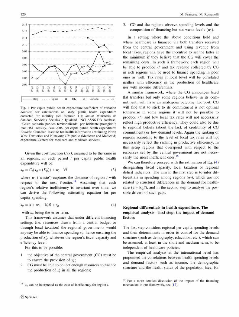
The level of within-country variation in Italy appears
lower than that observed for UK (Fig. 1), notwithstanding
the similarities in the organisation of the NHS system. It is
close to that in Spain where health expenditure is a
responsibility of regional governments as in Italy and to
that in Canada where healthcare is financed jointly by the
local and central government (via transfers and an equali-
sation programme). In the US, where the system is very
different and the role of the private sector significantly
more relevant, even public spending (in particular Medi-
care and Medicaid) shows much higher within country
variability (CBO [6]).
The reference model
We consider a benevolent regional government (i), which
wants to maximise the following:
maxxh;xu
p(KiÞUihðxi
h;KiÞþð1� p(KiÞÞUiuðxi
u;KiÞ ð1Þ
where
Uig : 9exg\1 such that Ui0
g ðxÞ\08 x [ exg g = h,u
Uhi is the utility of a healthy individual from the con-
sumption of healthcare (x) and Uui is the utility of a sick
one; xih and xi
u are the quantities of healthcare consumed
respectively by a healthy and a sick individual in region i; p
is the fraction of healthy individuals in the region and 1-p
the fraction of sick ones; Ki is a vector of economic, social,
demographic and health status characteristics that affect
both the probability of being sick and the preference
structure for the consumption of healthcare. We assume
that the budget constraint is either not binding13 or that the
regional government can draw additional resources from
the residents in the region to finance the production of the
optimal/desired health spending.
The optimal level of healthcare provision is:
x�i ¼ pxi�h þ ð1� pÞxi�
u ð2Þ
where xhi * and xu
i * solve problem (1).
8 For example, regarding the hospital sector, Iuzzolino [23] observes
that, compared with the other OECD countries, Italy has a larger share
of public hospitals of small size, probably because of poorer
outpatient care and an unbalanced allocation of resources between
different types of services. This is reflected in the unit costs of
hospitalisation and the share of outlays for hospital in total spending,
which are higher than the OECD average.9 For the details of the model estimation, see [17].10 Patient mobility among regions is allowed under the national
public healthcare system: healthcare costs are covered by the NHS
independently of the region actually providing the service.11 In order to compute per capita public current health expenditure
adjusted for patient mobility and the age structure of the population,
we have used population data (broken down by region and age) and
the coefficients published by Ministero della Salute [27], which
capture differences in the consumption of pharmaceuticals and
hospital services between individuals at different ages. We have then
adjusted expenditure to take into account population mobility (using
expenditure data for non-residents published yearly by Ministero
dell’Economia e delle finanze for each region) and finally computed
spending per capita values. For more details, see [17].
12 In particular, taking into account patient mobility and the age
structure of the population, the per-capita expenditure of the southern
regions in 2006 increases from 1,601 euros to 1,703 euros, while in
the Centre and the North it decreases from 1,735 euros to 1,680.13 This assumption is consisent with the literature on soft budget
constraints and with the evidence of systematic spending overruns and
deficits in the health sector.
An analysis of regional spending differentials in Italy 119
123
Given the cost function Ct(x), assumed to be the same in
all regions, in each period t per capita public health
expenditure will be:
sit ¼ Ctðxit � ðKitÞÞ þ wi 8i ð3Þ
where wi (‘waste’) captures the distance of region i with
respect to the cost frontier.14 Assuming that each
region’s relative inefficiency is invariant over time, we
can derive the following estimating equation for per
capita spending:
sit ¼ aþ wi þ k0itbþ eit ð4Þ
with eit being the error term.
This framework assumes that under different financing
settings (i.e. resources drawn from a central budget or
through local taxation) the regional governments would
anyway be able to finance spending sit, hence ensuring the
production of x�it, whatever the region’s fiscal capacity and
efficiency level.
For this to be possible:
1. the objective of the central government (CG) must be
to ensure the provision of x�i ;
2. CG must be able to collect enough resources to finance
the production of x�i in all the regions;
3. CG and the regions observe spending levels and the
composition of financing but not waste levels ðwiÞ.
In a setting where the above conditions hold and
where healthcare is financed via both transfers received
from the central government and using revenue from
local taxes, regions have the incentive to set the latter at
the minimum if they believe that the CG will cover the
remaining costs. In such a framework each region will
be able to produce x�i and tax revenue collected by CG
in rich regions will be used to finance spending in poor
ones as well. Tax rates at local level will be correlated
neither with efficiency in the production of healthcare
nor with income differentials.
A similar framework, where the CG announces fixed
flat transfers but only some regions believe in its com-
mitment, will have an analogous outcome. Ex post, CG
will find that to stick to its commitment is not optimal
(otherwise in some regions it will not be possible to
produce x�i ) and low local tax rates will not necessarily
reflect high productive efficiency. They could also be due
to regional beliefs (about the lack of credibility of CG
commitment) or low demand levels. Again the ranking of
regions according to the level of local tax rates will not
necessarily reflect the ranking in productive efficiency. In
this setup regions that overspend with respect to the
resources set by the central government are not neces-
sarily the most inefficient ones.15
We can therefore proceed with the estimation of Eq. (4)
disregarding fiscal capacity, local taxation or regional
deficit indicators. The aim in the first step is to infer dif-
ferentials in spending among regions (wi), which are not
related to structural differences in the demand for health-
care (aþ k0itb), and in the second step to analyse the pos-
sible drivers of such gaps.
Regional differentials in health expenditure. The
empirical analysis—first step: the impact of demand
factors
The first step considers regional per capita spending levels
and their determinants in order to control for the demand
structure (such as demography, education, etc.), which can
be assumed, at least in the short and medium term, to be
independent of healthcare policies.
The empirical analysis at the international level has
pinpointed the correlations between health spending levels
and demand factors such as income, the demographic
structure and the health status of the population (see, for
0.04
0.05
0.06
0.07
0.08
0.09
0.10
0.11
0.12
0.13
1992
1993
1994
1995
1996
1997
1998
1999
2000
2001
2002
2003
2004
2005
2006
Italy Spain UK Canada US
Fig. 1 Per capita public health expenditure-coefficient of variation
Sources: our calculations on: Italy: public health expenditure
corrected for mobility (see footnote 11); Spain: Ministerio de
Sanidad, Servicios Sociales e Igualdad, INCLASNS-DB database,
‘‘Gasto sanitario publico territorializado, por habitante protegido’’;
UK: HM Treasury, Pesa 2008, per capita public health expenditure;
Canada: Canadian Institute for health information (excluding North
West Territories and Nunavut); US: public (Medicare and Medicaid)
expenditure-Centers for Medicare and Medicaid services
14 wi can be interpreted as the cost of inefficiency for region i.
15 For a more detailed discussion of the impact of the financing
mechanism in our framework, see [17].
120 M. Francese, M. Romanelli
123
example, [18, 28]). Usually, most of the empirical literature
also controls for labour market and education indicators or
variables capturing institutional differences between
healthcare systems.16
We use a similar approach to investigate regional per
capita spending levels and in turn identify ‘‘unexplained’’
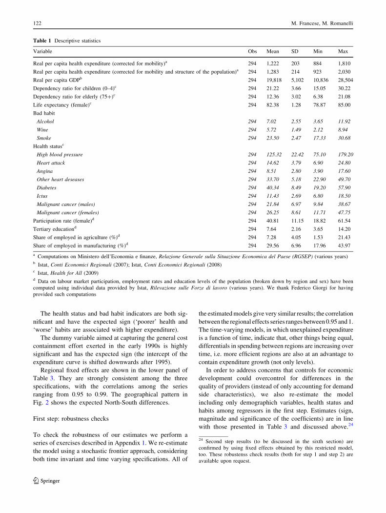
differentials. We use a panel of the 21 Italian regions for
14 years (1993–2006), which includes variables on per
capita health expenditure and its breakdown, per capita
GDP, health status indicators, variables relating to the
labour market and education (for descriptive statistics, see
Table 1).
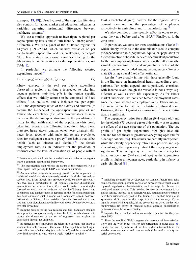
In particular, we estimate the following semilog
expenditure model:17
ln rexp pcitð Þ ¼ aþ g ið Þ þ x0itbþ eit ð5Þ
where rexp_pcit is the real per capita expenditure
observed in region i at time t (corrected to take into
account patients mobility), g(i) is the region specific
effects that we initially assume to be composed of fixed
effects,18 i.e. g(i) = ai, and x includes: real per capita
GDP; the dependency ratios of the elderly and children (to
capture the U-shape of the age-expenditure profile) and
female life expectancy (the latter two variables as indi-
cators of the demographic structure of the population); a
proxy for the health status of the population (this proxy
takes into account the following conditions: high blood
pressure, heart attack, angina, other heart diseases, dia-
betes, ictus, together with male and female prevalence
rates for malignant cancer); a proxy19 for habits that affect
health (such as tobacco and alcohol);20 the female
employment rate, as an indicator for the provision of
informal care; the level of education (% of people with at
least a bachelor degree); proxies for the regions’ devel-
opment measured as the percentage of employees
respectively in agriculture and in manufacturing.21
We also consider a time-specific effect in order to sep-
arate the years before and after 1995.22 Finally, eit is the
error term.
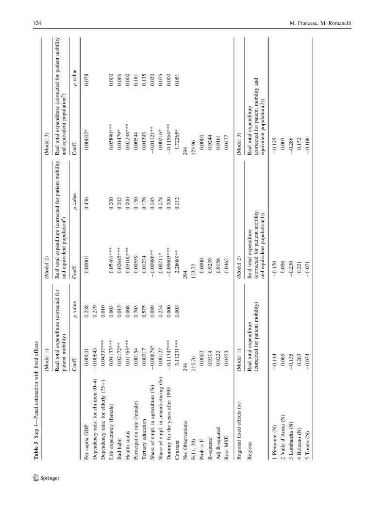
In particular, we consider three specifications (Table 3),
which simply differ as to the denominator used to compute
the dependent variable (population, equivalent population for
the consumption of hospital services or equivalent population
for the consumption of pharmaceuticals; in the latter cases the
variables accounting for the demographic structure of the
population are not included among the regressors). We esti-
mate (5) using a panel fixed effect estimator.
Results23 are broadly in line with those generally found
in the literature on international health expenditure com-
parisons. Per capita expenditure is positively correlated
with income (even though the variable is not always sig-
nificant) as well as with life expectancy. As for labour
market indicators, we consider female employment rates,
since the more women are employed in the labour market,
the more often formal care substitutes informal care.
However, the employment rate turns out to be not statis-
tically significant.
The dependency ratios for children (0–4 years old) and
for the elderly (75 years of age or older) allow us to capture
the effect of the age structure of the population. The age
profile of per capita expenditure highlights how the
demand for healthcare is greater at very young ages and for
older age cohorts [24]. The results are partially unexpected:
while the elderly dependency ratio has a positive and sig-
nificant sign, the dependency ratio of the very young is not
significant. This finding may be driven by considering too
broad an age class (0–4 years of age) as the expenditure
profile is higher at younger ages, particularly in infancy or
early childhood [8].
16 In our analysis we do not include the latter variables as the regions
share a common institutional framework.17 The specification used reflects the nature of the regressors. All of
them, apart from per capita GDP, are ratios or dummies.18 An alternative estimation strategy would be to implement a
multilevel model that simultaneously considers both the first and the
second step. Even though this procedure could be more efficient, it
has two main drawbacks: (1) it requires stronger distributional
assumptions on the error terms; (2) it would make it less straight-
forward to work out an estimate of the inefficiency levels and
decompose and analyse them as reported in the following paragraph.
We have estimated such a model as a robustness check, however;
estimated coefficients of the variables from the first and the second
step and their significance are in line with those obtained following a
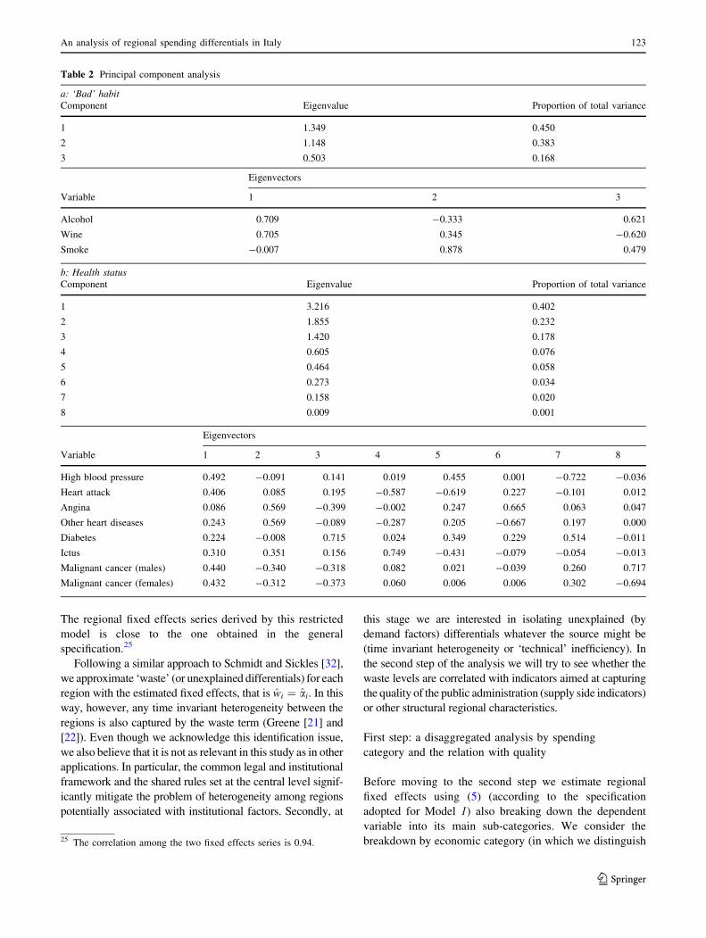
two-step procedure.19 Both the proxies for the health status and ‘bad’ habits are obtained
via a principal component analysis (see Table 2), which allows us to
reduce the dimension of the set of regressors and exploit the
correlation among the variables.20 In particular, the followings are taken into account: the share of
smokers (variable ‘smoke’), the share of the population drinking at
least half a litre of wine a day (variable ‘wine’) and the share of those
who drink alcohol at least twice a week (variable ‘alcohol’).
21 Including measures of development as demand factors may raise
some concerns about possible correlation between those variables and
regional supply-side characteristics, such as wage levels and the
quality of human capital. This problem however is quite minor in the
Italian setting. Indeed, (1) as concern wages, national labour contracts
have been used and are used in the Italian NHS so that there are no
systematic differences in this respect across the country; (2) as
regards human capital quality, hiring procedure are based on the same
requirements (in terms of medical school degrees, specialisation
patterns) across the whole country.22 In particular, we include a dummy variable equal to 1 for the years
after 1995.23 Since the modified Wald suggests the presence of heteroskedas-
ticity and the Wooldridge test for autocorrelation in panel data [35]
rejects the null hypothesis of no first order autocorrelation, the
standard error estimator used is robust to both hetoreskedasticity and
serial correlation.
An analysis of regional spending differentials in Italy 121
123
The health status and bad habit indicators are both sig-
nificant and have the expected sign (‘poorer’ health and
‘worse’ habits are associated with higher expenditure).
The dummy variable aimed at capturing the general cost
containment effort exerted in the early 1990s is highly
significant and has the expected sign (the intercept of the
expenditure curve is shifted downwards after 1995).
Regional fixed effects are shown in the lower panel of
Table 3. They are strongly consistent among the three
specifications, with the correlations among the series
ranging from 0.95 to 0.99. The geographical pattern in
Fig. 2 shows the expected North-South differences.
First step: robustness checks
To check the robustness of our estimates we perform a
series of exercises described in Appendix 1. We re-estimate
the model using a stochastic frontier approach, considering
both time invariant and time varying specifications. All of
the estimated models give very similar results; the correlation
between the regional effects series ranges between 0.95 and 1.
The time-varying models, in which unexplained expenditure
is a function of time, indicate that, other things being equal,
differentials in spending between regions are increasing over
time, i.e. more efficient regions are also at an advantage to
contain expenditure growth (not only levels).
In order to address concerns that controls for economic
development could overcontrol for differences in the
quality of providers (instead of only accounting for demand
side characteristics), we also re-estimate the model
including only demographich variables, health status and
habits among regressors in the first step. Estimates (sign,
magnitude and significance of the coefficients) are in line
with those presented in Table 3 and discussed above.24
Table 1 Descriptive statistics
Variable Obs Mean SD Min Max
Real per capita health expenditure (corrected for mobility)a 294 1,222 203 884 1,810
Real per capita health expenditure (corrected for mobility and structure of the population)a 294 1,283 214 923 2,030
Real per capita GDPb 294 19,818 5,102 10,836 28,504
Dependency ratio for children (0–4)c 294 21.22 3.66 15.05 30.22
Dependency ratio for elderly (75?)c 294 12.36 3.02 6.38 21.08
Life expectancy (female)c 294 82.38 1.28 78.87 85.00
Bad habit
Alcohol 294 7.02 2.55 3.65 11.92
Wine 294 5.72 1.49 2.12 8.94
Smoke 294 23.50 2.47 17.33 30.68
Health statusc
High blood pressure 294 125.32 22.42 75.10 179.20
Heart attack 294 14.62 3.79 6.90 24.80
Angina 294 8.51 2.80 3.90 17.60
Other heart deseases 294 33.70 5.18 22.90 49.70
Diabetes 294 40.34 8.49 19.20 57.90
Ictus 294 11.43 2.69 6.80 18.50
Malignant cancer (males) 294 21.84 6.97 9.84 38.67
Malignant cancer (females) 294 26.25 8.61 11.71 47.75
Participation rate (female)d 294 40.81 11.15 18.82 61.54
Tertiary educationd 294 7.64 2.16 3.65 14.20
Share of employed in agriculture (%)d 294 7.28 4.05 1.53 21.43
Share of employed in manufacturing (%)d 294 29.56 6.96 17.96 43.97
a Computations on Ministero dell’Economia e finanze, Relazione Generale sulla Situazione Economica del Paese (RGSEP) (various years)b Istat, Conti Economici Regionali (2007); Istat, Conti Economici Regionali (2008)c Istat, Health for All (2009)d Data on labour market participation, employment rates and education levels of the population (broken down by region and sex) have been
computed using individual data provided by Istat, Rilevazione sulle Forze di lavoro (various years). We thank Federico Giorgi for having
provided such computations
24 Second step results (to be discussed in the sixth section) are
confirmed by using fixed effects obtained by this restricted model,
too. These robustenss check results (both for step 1 and step 2) are
available upon request.
122 M. Francese, M. Romanelli
123
The regional fixed effects series derived by this restricted
model is close to the one obtained in the general
specification.25
Following a similar approach to Schmidt and Sickles [32],
we approximate ‘waste’ (or unexplained differentials) for each
region with the estimated fixed effects, that is wi ¼ ai. In this
way, however, any time invariant heterogeneity between the
regions is also captured by the waste term (Greene [21] and
[22]). Even though we acknowledge this identification issue,
we also believe that it is not as relevant in this study as in other
applications. In particular, the common legal and institutional
framework and the shared rules set at the central level signif-
icantly mitigate the problem of heterogeneity among regions
potentially associated with institutional factors. Secondly, at
this stage we are interested in isolating unexplained (by
demand factors) differentials whatever the source might be
(time invariant heterogeneity or ‘technical’ inefficiency). In
the second step of the analysis we will try to see whether the
waste levels are correlated with indicators aimed at capturing
the quality of the public administration (supply side indicators)
or other structural regional characteristics.
First step: a disaggregated analysis by spending
category and the relation with quality
Before moving to the second step we estimate regional
fixed effects using (5) (according to the specification
adopted for Model 1) also breaking down the dependent
variable into its main sub-categories. We consider the
breakdown by economic category (in which we distinguish
Table 2 Principal component analysis
a: ‘Bad’ habit
Component Eigenvalue Proportion of total variance
1 1.349 0.450
2 1.148 0.383
3 0.503 0.168
Eigenvectors
Variable 1 2 3
Alcohol 0.709 -0.333 0.621
Wine 0.705 0.345 -0.620
Smoke -0.007 0.878 0.479
b: Health status
Component Eigenvalue Proportion of total variance
1 3.216 0.402
2 1.855 0.232
3 1.420 0.178
4 0.605 0.076
5 0.464 0.058
6 0.273 0.034
7 0.158 0.020
8 0.009 0.001
Eigenvectors
Variable 1 2 3 4 5 6 7 8
High blood pressure 0.492 -0.091 0.141 0.019 0.455 0.001 -0.722 -0.036
Heart attack 0.406 0.085 0.195 -0.587 -0.619 0.227 -0.101 0.012
Angina 0.086 0.569 -0.399 -0.002 0.247 0.665 0.063 0.047
Other heart diseases 0.243 0.569 -0.089 -0.287 0.205 -0.667 0.197 0.000
Diabetes 0.224 -0.008 0.715 0.024 0.349 0.229 0.514 -0.011
Ictus 0.310 0.351 0.156 0.749 -0.431 -0.079 -0.054 -0.013
Malignant cancer (males) 0.440 -0.340 -0.318 0.082 0.021 -0.039 0.260 0.717
Malignant cancer (females) 0.432 -0.312 -0.373 0.060 0.006 0.006 0.302 -0.694
25 The correlation among the two fixed effects series is 0.94.
An analysis of regional spending differentials in Italy 123
123
Ta
ble
3S
tep
1—
Pan
eles
tim
atio
nw
ith
fix
edef
fect
s
(Mo
del
1)
(Mo
del
2)
(Mo
del
3)
Rea
lto
tal
exp
end
itu
re(c
orr
ecte
dfo
r
pat
ien
tm
ob
ilit
y)
Rea
lto
tal
exp
end
itu
re(c
orr
ecte
dfo
rp
atie
nt
mo
bil
ity
and
equ
ival
ent
po
pu
lati
on
a)
Rea
lto
tal
exp
end
itu
re(c
orr
ecte
dfo
rp
atie
nt
mo
bil
ity
and
equ
ival
ent
po
pu
lati
on
b)
Co
eff.
pv
alu
eC
oef
f.p
val
ue
Co
eff.
pv
alu
e
Per
cap
ita
GD
P0
.00
00
10
.24
80
.00
00
10
.43
60
.00
00
2*
0.0
78
Dep
end
ency
rati
ofo
rch
ild
ren
(0–
4)
-0
.00
64
50
.27
9
Dep
end
ency
rati
ofo
rel
der
ly(7
5?
)0
.04
33
7*
**
0.0
10
Lif
eex
pec
tan
cy(f
emal
e)0
.04
13
3*
**
0.0
03
0.0
54
61
**
*0
.00
00
.05
89
0*
**
0.0
00
Bad
hab
it0
.02
17
2*
*0
.01
50
.02
64
5*
**
0.0
02
0.0
14
79
*0
.06
6
Hea
lth
stat
us
0.0
17
63
**
*0
.00
80
.03
10
0*
**
0.0
00
0.0
22
98
**
*0
.00
0
Par
tici
pat
ion
rate
(fem
ale)
0.0
01
54
0.7
03
0.0
05
59
0.1
50
0.0
05
44
0.1
81
Ter
tiar
yed
uca
tio
n0
.00
31
70
.57
50
.01
23
40
.17
80
.01
39
30
.13
5
Sh
are
of
emp
l.in
agri
cult
ure
(%)
-0
.00
67
8*
0.0
89
-0
.00
98
6*
*0
.04
5-
0.0
11
21
**
0.0
20
Sh
are
of
emp
l.in
man
ufa
ctu
rin
g(%
)0
.00
12
70
.25
40
.00
21
1*
0.0
78
0.0
02
16
*0
.07
5
Du
mm
yfo
rth
ey
ears
afte
r1
99
5-
0.1
17
47
**
*0
.00
0-
0.0
96
03
**
*0
.00
0-
0.1
15
64
**
*0
.00
0
Co
nst
ant
3.1
12
31
**
*0
.00
32
.28
08
9*
*0
.01
21
.72
26
5*
0.0
51
No
.O
bse
rvat
ion
s2
94
29
42
94
F(1
1,
20
)1
15
.76
12
3.7
21
23
.96
Pro
b[
F0
.00
00
0.0
00
00
.00
00
R-s
qu
ared
0.9
30
40
.92
39
0.9
24
4
Ad
jR
-sq
uar
ed0
.92
22
0.9
15
60
.91
61
Ro
ot
MS
E0
.04
53
0.0
46
20
.04
77
Reg
ion
alfi
xed
effe
cts
(ai)
(Mo
del
1)
(Mo
del
2)
(Mo
del
3)
Reg
ion
sR
eal
tota
lex
pen
dit
ure
(co
rrec
ted
for
pat
ien
tm
ob
ilit
y)
Rea
lto
tal
exp
end
itu
re
(co
rrec
ted
for
pat
ien
tm
ob
ilit
y
and
equ
ival
ent
po
pu
lati
on
(1))
Rea
lto
tal
exp
end
itu
re
(co
rrec
ted
for
pat
ien
tm
ob
ilit
yan
d
equ
ival
ent
po
pu
lati
on
(2))
1P
iem
on
te(N
)-
0.1
44
-0
.17
0-
0.1
75
2V
alle
d’A
ost
a(N
)0
.06
50
.05
60
.00
7
3L
om
bar
dia
(N)
-0
.13
5-
0.2
30
-0
.28
6
4B
olz
ano
(N)
0.2
63
0.2
21
0.1
52
5T
ren
to(N
)-
0.0
34
-0
.07
1-
0.1
08
124 M. Francese, M. Romanelli
123
Ta
ble
3co
nti
nu
ed
Reg
ion
alfi
xed
effe
cts
(ai)
(Mo
del
1)
(Mo
del
2)
(Mo
del
3)
Reg
ion
sR
eal
tota
lex
pen
dit
ure
(co
rrec
ted
for
pat
ien
tm
ob
ilit
y)
Rea
lto
tal
exp
end
itu
re
(co
rrec
ted
for
pat
ien
tm
ob
ilit
y
and
equ
ival
ent
po
pu
lati
on
(1))
Rea
lto
tal
exp
end
itu
re
(co
rrec
ted
for
pat
ien
tm
ob
ilit
yan
d
equ
ival
ent
po
pu
lati
on
(2))
6V
enet
o(N
)-
0.1
31
-0
.19
9-
0.2
14
7F
riu
liV
enez
iaG
iuli
a(N
)-
0.2
51
-0
.25
2-
0.2
33
8L
igu
ria
(N)
-0
.27
0-
0.2
01
-0
.15
9
9E
mil
iaR
om
agn
a(N
)-
0.2
78
-0
.30
5-
0.3
03
10
To
scan
a(C
)-
0.2
60
-0
.25
4-
0.2
49
11
Um
bri
a(C
)-
0.2
45
-0
.26
1-
0.2
21
12
Mar
che
(C)
-0
.22
7-
0.2
59
-0
.24
2
13
Laz
io(C
)0
.10
40
.04
5-
0.0
00
14
Ab
ruzz
o(S
)-
0.0
34
-0
.01
8-
0.0
04
15
Mo
lise
(S)
0.0
17
0.0
79
0.1
23
16
Cam
pan
ia(S
)0
.41
20
.43
40
.43
7
17
Pu
gli
a(S
)0
.25
90
.30
40
.31
5
18
Bas
ilic
ata
(S)
0.1
39
0.1
88
0.2
23
19
Cal
abri
a(S
)0
.22
30
.25
90
.30
0
20
Sic
ilia
(S)
0.2
85
0.3
52
0.3
72
21
Sar
deg
na
(S)
0.2
43
0.2
80
0.2
66
*,
**
,*
**
Sig
nifi
can
ceat
10
,5
and
1%
lev
el(s
tan
dar
der
rors
rob
ust
toh
eter
osk
edas
tici
tyan
dau
toco
rrel
atio
n);
(N)
No
rth
,(C
)C
entr
e;(S
)S
ou
tha
Usi
ng
wei
gh
tsfo
rh
osp
ital
serv
ices
bU
sin
gw
eig
hts
for
ph
arm
aceu
tica
lco
nsu
mp
tio
n
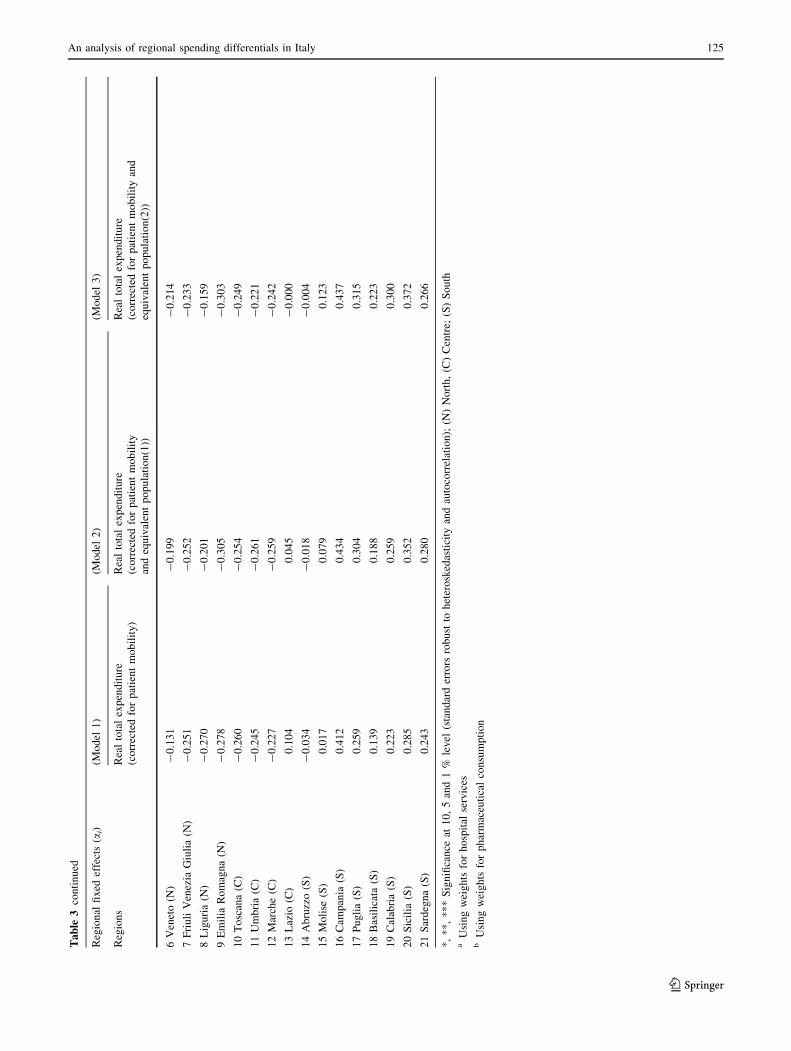
An analysis of regional spending differentials in Italy 125
123
between wages, purchases of goods and services, spending
for private hospitals recognised within the NHS, primary
care, pharmaceuticals, and specialised care).26
Given the estimates for each expenditure category we
can recover aggregate regional ‘waste levels’. Assuming
that each expenditure item h presents a relationship as in
(5) and using the same set of regressors, i.e. E chit
� �
¼ex0 itb
hþahþahi ; h ¼ 1; . . .;H (H being the total number of
expenditure items), we have that:
ex0 itbþaþai ¼X
H
h¼1
ex0 itbhþahþah
i ð6Þ
From this it follows that:
eai�aimin
|fflfflffl{zfflfflffl}
ni
¼X
H
h¼1
ex0itbhþah
ex0itbþa
|fflfflffl{zfflfflffl}
shi
eahi
eaimin|ffl{zffl}
~nhi
ð7Þ
The distance to the minimum cost for each region i can be
represented as a weighted average of the inefficiency scores
for each expenditure item ð~nhi Þ, with the latter normalised
with respect to the minimum total regional effect. Estimated
fixed effects obtained by aggregating the results for the
expenditure items are in line with those obtained estimating
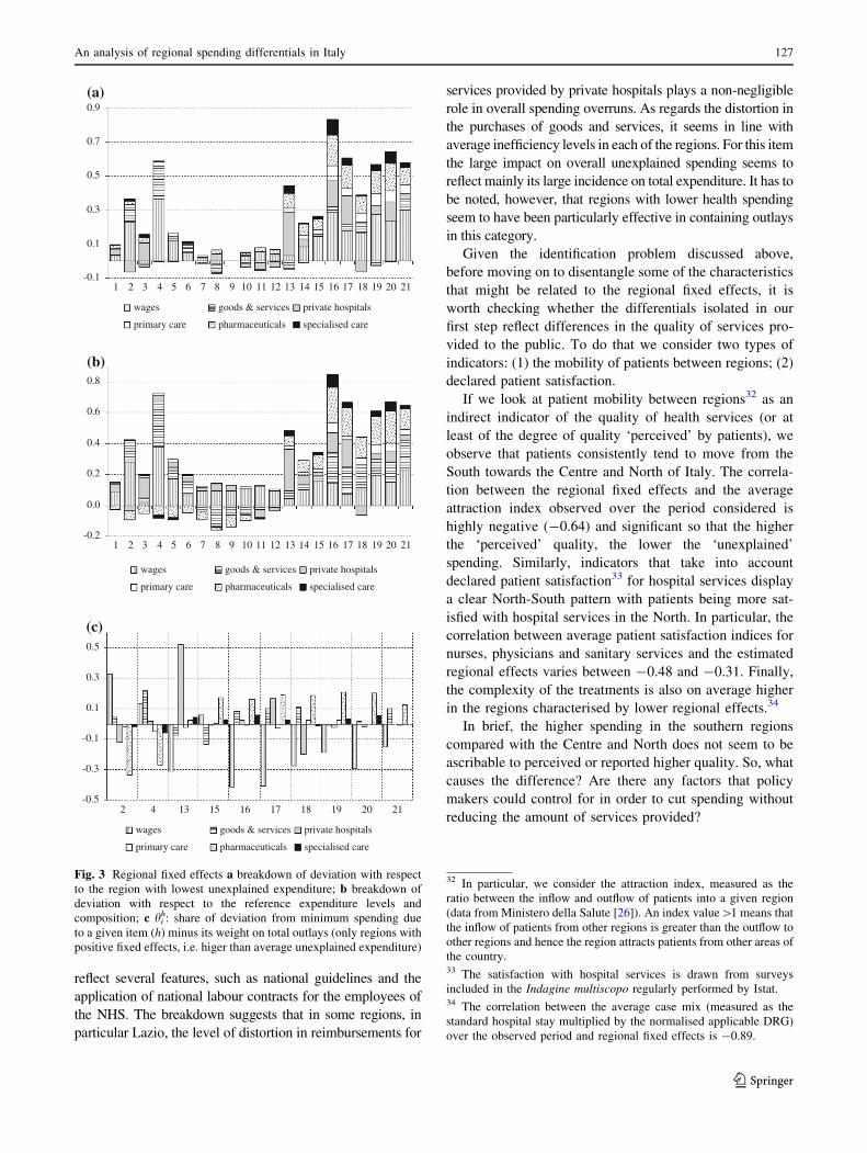
aggregate expenditure.27 Figure 3a shows for each region the
contribution of each expenditure item to the difference
between its own inefficiency score and the minimum one
Di ¼ ðni � nminÞ.28 Figure 3b instead shows the contribution
of each expenditure item to the difference between the actual
inefficiency score and the score that would have occurred in
region i had all the ~nhi been equal to 1.29
This decomposition allows us to point out some interesting
patterns. Low levels of unexplained expenditure (characterised
by Di equal or close to 0) seem compatible with different
choices as regards spending composition. Furthermore, in
regions with higher spending the distribution of inefficiency
among expenditure items does not seem to be uniform. In
particular, in the regions with a positive total fixed effect
(meaning, ceteris paribus, higher than average unexplained
expenditure), the management of the outlays that account for
relatively smaller shares of the budget seems in need of par-
ticularly careful monitoring. This is evident if we consider the
distribution of the inefficiency among expenditure items
computing #hi ¼
~Dhi
Di� sh
i , an indicator that compares the share
of the deviation from minimum spending because of a given
expenditure item and the reference share of that same item in
total outlays (Fig. 3c).30 For the southern regions with a
positive total fixed effect, the distortion in spending on phar-
maceuticals is particularly relevant, while the weight of the
inefficiency in hospital spending is less pronounced than
implied by their reference share of total spending.31 This might
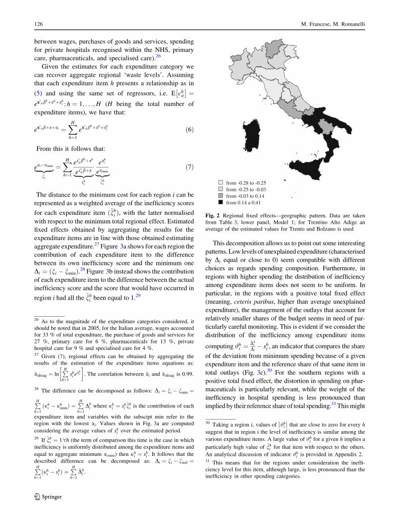
from -0.28 to -0.25from -0.25 to -0.03from -0.03 to 0.14from 0.14 a 0.41
Fig. 2 Regional fixed effects—geographic pattern. Data are taken
from Table 3, lower panel, Model 1; for Trentino Alto Adige an
average of the estimated values for Trento and Bolzano is used
26 As to the magnitude of the expenditure categories considered, it
should be noted that in 2005, for the Italian average, wages accounted
for 33 % of total expenditure, the purchase of goods and services for
27 %, primary care for 6 %, pharmaceuticals for 13 %, private
hospital care for 9 % and specialised care for 4 %.27 Given (7), regional effects can be obtained by aggregating the
results of the estimation of the expenditure items equations as:
aidisag ¼ lnP
H
h¼1
shi eah
i
� �
. The correlation between ai and aidisag is 0.99.
28 The difference can be decomposed as follows: Di ¼ ni � nmin ¼
P
H
h¼1
ðjhi � jh
iminÞ ¼P
H
h¼1
Dhi where jh
i ¼ shi~nh
i is the contribution of each
expenditure item and variables with the subscipt min refer to the
region with the lowest ai. Values shown in Fig. 3a are computed
considering the average values of shi over the estimated period.
29 If ~nhi ¼ 18h (the term of comparison this time is the case in which
inefficiency is uniformly distributed among the expenditure items and
equal to aggregate minimum ai min) then jhi ¼ sh
i . It follows that the
described difference can be decomposed as: Di ¼ ni � niref ¼P
H
h¼1
ðjhi � sh
i Þ ¼P
H
h¼1
~Dhi .
30 Taking a region i, values of #hi
�
�
�
� that are close to zero for every h
suggest that in region i the level of inefficiency is similar among the
various expenditure items. A large value of #hi for a given h implies a
particularly high value of ~nhi for that item with respect to the others.
An analytical discussion of indicator #hi is provided in Appendix 2.
31 This means that for the regions under consideration the ineffi-
ciency level for this item, although large, is less pronounced than the
inefficiency in other spending categories.
126 M. Francese, M. Romanelli
123
reflect several features, such as national guidelines and the
application of national labour contracts for the employees of
the NHS. The breakdown suggests that in some regions, in
particular Lazio, the level of distortion in reimbursements for
services provided by private hospitals plays a non-negligible
role in overall spending overruns. As regards the distortion in
the purchases of goods and services, it seems in line with
average inefficiency levels in each of the regions. For this item
the large impact on overall unexplained spending seems to
reflect mainly its large incidence on total expenditure. It has to
be noted, however, that regions with lower health spending
seem to have been particularly effective in containing outlays
in this category.
Given the identification problem discussed above,
before moving on to disentangle some of the characteristics
that might be related to the regional fixed effects, it is
worth checking whether the differentials isolated in our
first step reflect differences in the quality of services pro-
vided to the public. To do that we consider two types of
indicators: (1) the mobility of patients between regions; (2)
declared patient satisfaction.
If we look at patient mobility between regions32 as an
indirect indicator of the quality of health services (or at
least of the degree of quality ‘perceived’ by patients), we
observe that patients consistently tend to move from the
South towards the Centre and North of Italy. The correla-
tion between the regional fixed effects and the average
attraction index observed over the period considered is
highly negative (-0.64) and significant so that the higher
the ‘perceived’ quality, the lower the ‘unexplained’
spending. Similarly, indicators that take into account
declared patient satisfaction33 for hospital services display
a clear North-South pattern with patients being more sat-
isfied with hospital services in the North. In particular, the
correlation between average patient satisfaction indices for
nurses, physicians and sanitary services and the estimated
regional effects varies between -0.48 and -0.31. Finally,
the complexity of the treatments is also on average higher
in the regions characterised by lower regional effects.34
In brief, the higher spending in the southern regions
compared with the Centre and North does not seem to be
ascribable to perceived or reported higher quality. So, what
causes the difference? Are there any factors that policy
makers could control for in order to cut spending without
reducing the amount of services provided?
-0.1
0.1
0.3
0.5
0.7
0.9
wages goods & services private hospitals
primary care pharmaceuticals specialised care
-0.2
0.0
0.2
0.4
0.6
0.8
wages goods & services private hospitals
primary care pharmaceuticals specialised care
(c)
-0.5
-0.3
-0.1
0.1
0.3
0.5
1 2 3 4 5 6 7 8 9 10 11 12 13 14 15 16 17 18 19 20 21
1 2 3 4 5 6 7 8 9 10 11 12 13 14 15 16 17 18 19 20 21
2 4 13 15 16 17 18 19 20 21
wages goods & services private hospitals
primary care pharmaceuticals specialised care
(b)
(a)
Fig. 3 Regional fixed effects a breakdown of deviation with respect
to the region with lowest unexplained expenditure; b breakdown of
deviation with respect to the reference expenditure levels and
composition; c hih: share of deviation from minimum spending due
to a given item (h) minus its weight on total outlays (only regions with
positive fixed effects, i.e. higer than average unexplained expenditure)
32 In particular, we consider the attraction index, measured as the
ratio between the inflow and outflow of patients into a given region
(data from Ministero della Salute [26]). An index value[1 means that
the inflow of patients from other regions is greater than the outflow to
other regions and hence the region attracts patients from other areas of
the country.33 The satisfaction with hospital services is drawn from surveys
included in the Indagine multiscopo regularly performed by Istat.34 The correlation between the average case mix (measured as the
standard hospital stay multiplied by the normalised applicable DRG)
over the observed period and regional fixed effects is -0.89.
An analysis of regional spending differentials in Italy 127
123
The empirical analysis—second step: the drivers
of regional differentials
The second step of our analysis tries to address this issue.
We investigate the correlation between regional effects and
some supply factors and regional characteristics that could
affect the unexplained variability observed in spending
levels. Italian regions, which operate in a context of
administrative autonomy, have the possibility to choose
different organisational arrangements within a common
legal and institutional framework that mandates them to
provide homogeneous healthcare coverage.35
The analysis exploits the result of the expenditure levels
estimation in step one. In particular, we consider the
covariates of the regional fixed effects estimating the fol-
lowing linear model:36
ai ¼ q0idþ fi i ¼ 1; . . .;N ð8Þ
where fi is the standard i.i.d. error term and qi is a
vector of j regressors and includes indicators for the
following categories: (1) appropriateness of treatments;37
(2) supply structure characteristics;38 (3) quality in public
administration39; (4) social capital.40 In order to
corroborate the idea that variables used in the second
stage reflect supply side characteristics, and not a com-
bination of supply and demand factors, we checked
whether there is any correlation with demand side driv-
ers (such as population age structure and health status,
using the same proxies employed in step 1 of our
analysis). Results suggest that no significant correlation
can be found.
Given the small number of observations, we started by
considering one (or at most two) regressor for each cate-
gory: the index for Caesarean sections, the index for total
employment and its composition; the indicator for general
practitioners with a large number of patients; the ratio
between the number of beds in private and public hospitals;
the share of the use of generic pharmaceuticals and proxies
for social capital (Table 4). To check the robustness of the
results, we also considered each category at a time and
substituted the proxy/ies included in the estimated speci-
fication. Table 4 also shows the results of a SURE model
having as dependent variables the regional effects for the
categories of hospital spending, primary care, outlays for
pharmaceuticals and specialised care.41
The appropriateness index turns out to be significantly
related to unexplained spending differentials; the higher the
inappropriateness is, the higher the regional effects. Inap-
propriateness characterises healthcare treatments that could
be performed ensuring at least the same effectiveness for
the patient, but incurring lower risks and/or employing a
lower amount of resources. Following the literature and
policy practice (see OECD [30], WHO [19], Francese et al.
[16] and references therein) as an indicator for appropri-
ateness, we have used Caesarean section rates at the
regional level. Results are confirmed even when we sub-
stitute Caesarean sections with inappropriate surgical ward
use index.42
As to supply indicators, we include both indexes related
to hospital organisation and to primary care, which are
directly established by policy makers according to national
and regional rules. As concerns the former, we find that a
35 Compensation of employees represents an exception; wages are set
by national labour contracts (however regions can decide on the
number and composition of employees).36 This is consistent with the assumption of regional effects being
time invariant. As seen above, the time invariant component
estimated using time varying frontier models or fixed effects gives
equivalent results. Apart from the common impact due to the
decaying factor, estimated waste levels are strongly correlated using
the four estimation procedures discussed in Appendix 1.37 The indicators considered under this category are the average over
the observed period of the incidence of Caesarian sections and of the
incidence of patients discharged by a surgical ward with a medical
DRG (data from Ministero della Salute [26]).38 In this category we considered the averages of the incidence of
NHS employees on residents; composition of employees (ratio of
medical staff over total employees); incidences of public hospital
beds on residents; incidences of private hospital beds; ratio between
number of beds in private to public hospitals; share of expenditure for
care provided by private hospitals; average stay in public hospitals;
average stay in private hospitals; number of general pratictioners;
number of patients per general pratictioner; number of general
pratictioners with more than 1,500 patients. All the data are drawn
from ISTAT, Health for All.39 To proxy the quality of administration we consider: the share of
pharmaceutical expenditure for generic (off-patent) pharmaceuticals
and the share of expenditure for pharmaceuticals delivered directly by
the NHS in total pharmaceutical expenditure. We also consider an
indicator for the use of IT in other Italian local governments in each
region; in particular, we use a municipality IT index, which is given
by the share of municipalities whose general registry office has been
computerised.40 In particular, we consider several proxies for social capital
commonly used in the literature: incidence of blood donors per
1,000 residents; incidence of recyclable waste collection; average
turnout at referenda; interest in politics and morality. The indicators
Footnote 40 continued
for solidarity/‘morality’ and participation/‘interest in politics’ are
drawn from Giordano et al. [20]. In particular, solidarity/‘morality’ is
a composite index summarising self-reported pro-social attitudes and
objective measures of altruistic behaviour (such as blood donation);
similarly, interest in politics is built from self-reported answers and
more objective measures (such as referendum participation).41 All the estimated models exclude the constant term. In fact, the
mean value of the fixed effects is zero by construction. To check for
this, however, we also replicate the estimation including the constant
term, which turns out to be not significant. Moreover, neither the sign
nor the magnitude of the estimated coefficients are affected by
including/excluding the constant.42 In this case, however, it interferes with the significance of the
number of employees indicator.
128 M. Francese, M. Romanelli
123
Ta
ble
4S
tep
2—
Dri
ver
so
fre
gio
nal
effe
cts
Reg
ion
alfi
xed
effe
cta
To
tal
exp
end
itu
re
Co
eff.
pv
alu
e
%C
aesa
rian
sect
ion
s0
.01
79
**
*0
.00
0
Inci
den
ceo
fN
HS
emp
l.o
nre
sid
ents
0.0
48
5*
**
0.0
02
Co
mp
osi
tio
no
fem
pl.
(med
ical
staf
f/em
pl.
)-
0.0
06
60
.23
2
GP
sw
ith
mo
reth
an1
50
0p
atie
nts
0.0
08
8*
**
0.0
00
#b
eds
inp
riv
ate/
#b
edin
pu
bli
ch
osp
ital
s0
.00
21
0.1
37
%g
ener
icd
rug
s-
0.0
54
5*
**
0.0
04
Inte
rest
inp
oli
tics
-0
.01
55
**
*0
.00
1
So
lid
arit
y0
.00
81
**
0.0
18
No
.O
bse
rvat
ion
s2
1
F(8
,1
3)
22
.07
Pro
b[
F0
.00
00
q y,y
20
.93
32
Reg
ion
alfi
xed
effe
ctb
Ho
spit
alex
pen
dit
ure
Pri
mar
yca
reP
har
mac
euti
cals
Sp
ecia
lise
dca
re
Co
eff.
pv
alu
eC
oef
f.p
val
ue
Co
eff.
pv
alu
eC
oef
f.p
val
ue
%C
aesa
rian
sect
ion
s0
.01
02
**
*0
.00
00
.00
17
**
*0
.00
00
.00
33
**
*0
.00
00
.00
10
**
0.0
27
Inci
den
ceo
fN
HS
emp
l.o
nre
sid
ents
0.0
48
9*
**
0.0
00
0.0
05
1*
**
0.0
00
0.0
04
6*
0.0
61
-0
.00
07
0.7
31
Co
mp
osi
tio
no
fem
pl.
(med
ical
staf
f/em
pl.
)0
.00
43
0.2
52
0.0
00
00
.95
40
.00
17
*0
.09
20
.00
01
0.9
18
GP
sw
ith
mo
reth
an1
50
0p
atie
nts
0.0
07
6*
**
0.0
00
0.0
00
4*
**
0.0
03
0.0
00
5*
*0
.03
50
.00
01
0.5
04
#b
eds
inp
riv
ate/
#b
edin
pu
bli
ch
osp
ital
s0
.00
16
*0
.09
50
.00
03
**
0.0
20
0.0
00
6*
*0
.02
90
.00
03
0.1
24
%g
ener
icd
rug
s-
0.0
39
9*
**
0.0
01
-0
.00
17
0.3
16
-0
.00
62
**
0.0
44
-0
.00
24
0.3
34
Inte
rest
inp
oli
tics
-0
.01
14
**
*0
.00
0-
0.0
01
4*
**
0.0
00
-0
.00
27
**
*0
.00
0-
0.0
00
80
.15
6
So
lid
arit
y0
.00
79
**
*0
.00
00
.00
05
*0
.10
00
.00
12
**
0.0
48
0.0
00
9*
0.0
58
No
.O
bse
rvat
ion
s2
12
12
12
1
F(8
,1
3)
55
9.1
41
84
.66
24
4.2
20
.15
Pro
b[
F0
.00
00
0.0
00
00
.00
00
0.0
00
0
q y,y
20
.99
71
0.9
91
30
.99
34
0.9
25
4
*,
**
,*
**
Sig
nifi
can
ceat
resp
ecti
vel
y1
0,
5an
d1
%le
vel
aO
rdin
ary
leas
tsq
uar
eb
Max
imu
mli
kel
iho
od
seem
ing
lyu
nre
late
dre
gre
ssio
n.
Sm
all
sam
ple
stat
isti
csar
eco
mp
ute
d
An analysis of regional spending differentials in Italy 129
123
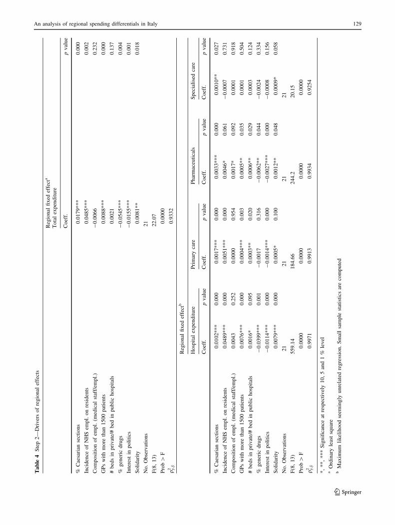
higher number of employees is related to higher spending,
as expected. Instead, the coefficient of the proxy for the
composition of the staff is not significant. Proxies (either
the ratio of beds in private to public hospitals or the share
of spending for private hospitals in total spending) for the
relevance of the private sector display a positive but not
significant coefficient in the regression for aggregate
regional effects; the coefficient is significant, however, in
the estimation of spending categories, in particular hospi-
tals, primary care and pharmaceuticals.
As regards primary care, the workload of general prac-
titioners (GPs) is significant; in particular, the share of
practitioners with a very large number of patients is related
to higher spending (the same happens when considering the
average number of patients for GP). Interestingly, the
workload of GPs also affects other spending items (besides
primary care); in fact, it is found that doctors workload has
a strong positive impact on hospital and pharmaceutical
spending as well as spending for primary care. This sug-
gests that too many patients to follow might make it more
difficult for general practitioners to avoid unnecessary
access to hospital services and use of pharmaceuticals.
Furthermore, it highlights that the overall organisation of
the system matters, since outlays in different categories are
related. As noted above when discussing first step results,
different expenditure compositions seem to be compatible
with overall efficiency.
To proxy the quality of administration we consider
indicators of practices that are aimed at reducing the
resources absorbed by consumption of pharmaceutical
without reducing the quantity provided or the effectiveness
of the treatments. These variables are intended to capture
good management by public authorities since they reflect
attention in providing effective services at reduced costs
(by reducing, for example, transaction costs or those
associated to branded drugs). In particular, we focus on the
share of pharmaceutical expenditure for generic (off-pat-
ent) drugs and the share of expenditure for pharmaceuticals
delivered directly by the NHS in total pharmaceutical
expenditure. As expected, indicators for good practices (we
considered alternatively the two indexes) do display a
negative relation to unexplained spending.
Finally, we also included in our model proxies for
informal rules and habits that might play a role in the
performances of different public administrations. The
economic literature often highlights the impact of history
and economic institutions on the development of different
regions. Institutions also include informal rules and con-
straints that are often summarised in the concept of social
capital.43 In this context, social capital captures the level of
trust and habits of cooperation shared among members of a
local community. As to our results, social capital indicators
turn out to be significant when splitting the two aspects of
solidarity/‘morality’ and participation/‘interest in politics’,
the first one being positively related to spending—probably
reflecting a higher propensity to share fundamental ser-
vices–the second one being negatively related to regional
effects—suggesting that the more public attention is given
to policy makers’ activity, the stronger their incentive to
manage the available resources efficiently.
Although the second step of the empirical analysis is
based on a small sample size, the correlations we detect are
sufficiently robust to derive some general policy consid-
erations. Regional spending differentials seem to be related
to both persistent (sticky?) regional features (such as social
capital) and characteristics that in the medium term can be
controlled by policy makers (such as the appropriateness of
health treatments, the workload of general practitioners or
the use of generics). Spreading administrative best prac-
tices and enhancing the degree of appropriateness of
treatments would be an effective way of reducing spending
differentials and increasing efficiency in the use of public
funds. Even relatively limited improvements could turn
into substantial savings: given our results, an increase in
the appropriateness level or in the use of generics by 1
percentage point44 implies on average a reduction of
respectively 1.8 and 5.3 % in total expenditure (€20.9 and
€62.3 per capita).
Concluding remarks
Several studies have documented the presence of regional
differentials in public health spending. The aim of this
work is to contribute to this discussion by analysing the
determinants of per capita health expenditure focussing on
identifying the drivers of inefficiency for the panel of
Italian regions and the existence of potential room for
savings. The article presents an empirical analysis of per
capita expenditure levels that takes into account the
regional differences in the need for health services. The
remaining differences in spending (the ‘‘unexplained dif-
ferentials’’) are then studied in relation to structural char-
acteristics and policy variables.
First, the results confirm the existence of potential
margins for savings that are related at least in part to dif-
ferences in the effectiveness of public administration.
However, with respect to previous studies, our methodol-
ogy not only allows us to evaluate the overall inefficiency
43 See Putnam [31], de Blasio and Nuzzo [9].
44 These computations use the result of the estimation of Model 1 in
Table 3 and the coefficents reported in the first column of Table 4.
Values are computed using variable averages over the regions and the
years 1993–2006.
130 M. Francese, M. Romanelli
123
level for every region, but also to estimate the contribution
of each spending item (e.g. wages, pharmaceuticals, etc.) to
that inefficiency. For all the regions, the analysis further
breaks it down into two factors: the first accounts for the
budget share of each spending category; the second cap-
tures its relative inefficiency. In our framework it is thus
possible to single out the categories that need careful
monitoring in the regions with poorer performances, such
as outlays for pharmaceuticals.
The second step of the study suggests that there are
policy tools (e.g. the use of generic drugs or the workload
of general practitioners) that might help to keep ineffi-
ciency under control. Moreover, some supply structure
indicators and proxies for good practices seem to be par-
ticularly important for certain spending categories.
Acknowledgments We thank two anonymous referees for their
comments, the discussants and the participants at conferences and
seminars where previous versions of this work were presented, and
the colleagues at the Public Finance Division of the Bank of Italy. The
usual disclaimers apply.
Appendix 1: Robustness checks
To check the robustness of our estimates, we run a series of
exercises. We estimate model 1 using alternative estima-
tion techniques. We start by considering a stochastic
frontier model45 of the type:
cit ¼ f ðxitÞnit ð9Þ
where nit ¼ 1 for the best unit in the sample and nit [ 1 for
the others.
We specify the efficient expenditure function as
f ðxitÞ ¼ econsþx0 itb ð10Þ
and hence we can write the estimating equation as
ln cit ¼ consþ x0itbþ uit þ mit ð11Þ
where mit iid Nð0; r2mÞ is the error term and
uit iid Nþðl; r2uÞ captures each region’s distance with
respect to the efficient frontier46:
nit ¼ euit ð12Þ
Initially, we assume that the stochastic frontier is invariant
over time.47 We then consider a time varying version a la
Battese and Coelli [1]:
uit ¼ e�gðt�TÞui with uitiidNþðl; r2uÞ ð13Þ
where the distance from minimum cost can be decomposed
into two factors, a given level of inefficiency ui charac-
terising each region and a time varying component, which
is a function of time and a decay factor g.
We also estimate a fixed effect model with time varying
regional effects. In particular, we derive an estimating
equation equivalent to the time varying stochastic frontier
described above (13). In this case the expenditure equation
becomes48:
ln cit ¼ x0itbþ e�gt/i þ eit with
/i ¼ ½egTai� ð14Þ
Using the approximation
e�gt ffi 1� gt þ g2 t2
2ð15Þ
we derive the following estimating equation49:
ln cit ¼ x0itbþ /i � gt/i þ g2 t2/i
2þ eit ð16Þ
From the estimates of (16) we can recover the parameters we
are interested in: the regional (time invariant) effects ai and
the decay factor g. In both time-varying models the estimated
decay factor is negative and significant. This might reflect a
common increasing pattern in health expenditure that could
be due to the impact of technological developments in the
production of healthcare, in the organisation at national level
of the health system or in the structure of preferences.
Appendix 2: Indicator for the distribution
of inefficiency among expenditure items
The indicator #hi can be rewritten as follows:
hhi ¼
shi~nh
i � shi
ni � niref
� shi or
hhi ¼ sh
i
~nhi � ni
ni � niref
ð17Þ
45 A drawback of this approach, however, is that using stochastic
frontiers requires explicit assumptions in terms of the distributions
involved.46 In general, model (11) can be related to model (5). In particular,
rearranging the estimating equation for model (5) with regional fixed
effects, we have that: ln rexp pcitð Þ ¼ aþmin aið Þ½ � þa�min aið Þ½ � þ x0itbþ eit with 0� ai �minðaiÞ ¼ ainorm� þ1,
which can be directly compared to (11) where 0� uit � þ1captures the inefficiency levels.
47 So that in terms of model (5) and rearranging the time invariant
fixed effects, the estimation of ai-min(ai) is analogous to the
estimation of ui.48 In terms of rearranging model (5) it is like writing: aitnorm ¼e�gðt�TÞainorm ¼ e�gðt�TÞai � e�gðt�TÞðminðaiÞÞ with ainorm ¼ 0 for the
best unit in the sample.49 This specification is analagous to those discussed in Cornwell et al.
[7] and Kumbhakar [25], where the authors suggest substituting a
constant inefficiency parameter with a quadratic specification as in
(16).
An analysis of regional spending differentials in Italy 131
123
when ~nhi ¼ ni 8h then hh
i ¼ 0 8h. All the items have the
same level of inefficiency. The distortion might be very big
but it is uniformly distributed among the expenditure
items. On the other hand, consider a case in which all
the first h–1 items are characterised by ‘full efficiency’ so
that ~nhi ¼ 1 8h ¼ 1; . . .;H � 1. In this case with
niref ¼P
H
h¼1
shi ¼ 1, we will have hh
i ¼ �shi 8h ¼ 1; . . .;
H � 1 while the overall inefficiency will reflect the
distortion in the last expenditure item: hHi will be
[ 0 [ hhi 8h ¼ 1; . . .;H � 1. Given (7), we will in fact
have that: ni ¼P
H�1
h¼1
shi
�
þ sHi
~nHi . Finally it should be
noted that for items characterised by ~nhi [ ni; h
hi will be
positive, while for ~nhi \ni; h
hi will be negative. This means
that a large distortion in a relatively small spending item
might be compensated by a relatively smaller distortion in
a spending item that accounts for a large fraction of total
outlays.
References
1. Battese, G., Coelli, T.: Frontier production functions, technical
efficiency and panel data: with application to paddy farmers in
India. J. Prod. Anal. 3, 153–169 (1992)
2. Bodenheimer, T., Berry-Millet, R.: Follow the money—control-
ling expenditure by improving care for patients needing costly
services. N. Engl. J. Med. 361, 1521–1523 (2009)
3. Bordignon, M., Turati, G.: Bailing out expectations and public
health expenditure. J.Health Econ. 28, 305–321 (2009)
4. Cantanero Prieto D., Lago-Penas S.: Decomposing the determi-
nants of health care expenditure: the case of Spain. Eur. J. Health
Econ. 13, 19–27 (2012)
5. Caroppo, M.S., Turati, G.: I sistemi sanitari regionali in Italia.
Milano, Vita e Pensiero (2007)
6. Congressional Budget Office: Geographic variation in health care
spending. CBO Paper 2978. Washington DC. (2008)
7. Cornwell, C., Schmidt, P., Sickles, R.: Production frontiers with
cross sectional and time series variation in efficiency levels.
J. Econom. 46, 185–200 (1990)
8. Cutler D. M., Meara E.: The medical costs of the young and the
old: a forty year perspective, NBER Working Papers 6114.
Cambridge (MA). (1997)
9. de Blasio G., Nuzzo G.: The legacy of history for economic
development: the case of Putnam’s social capital. Temi di Dis-
cussione, 591. Banca d’Italia, Roma. (2006)
10. De Matteis, P., Messina, G.: Le capacita fiscali delle Regioni
italiane. Rivista economica del Mezzogiorno 3, 363–396 (2010)
11. Economic Policy Committee, European Commission: The 2009
ageing report: economic and budgetary projections for the EU-27
member states (2008–2060). Eur. Econ., 2 (2009)
12. Fisher, E.S., Bynum, J.P., Skinner, J.S.: Slowing the growth of
healthcare costs—lessons from regional variation. N. Engl.
J. Med. 360, 849–852 (2009)
13. Fisher, E.S., Wennberg, D.E., Stukel, T.A., Gottlieb, D.J., Lucas,
F.L., Pinder, E.L.: The implication of regional variations in
Medicare spending. Part 1: the content, quality, and accessibility
of care. Ann. Intern. Med. 138(4), 273–311 (2003)
14. Fisher, E.S., Wennberg, D.E., Stukel, T.A., Gottlieb, D.J., Lucas,
F.L., Pinder, E.L.: The implication of regional variations in
Medicare spending. Part 2: health outcomes and satisfaction with
care. Ann. Intern. Med. 138(4), 288–322 (2003)
15. Fowler, F.J., Gallagher, P.M., Anthony, D.L., Larsen, K., Skin-
ner, J.S.: Relationship between regional per capita medicare
expenditures and patient perceptions of quality of care. J. Am.
Med. Assoc. 299, 2406–2412 (2008)
16. Francese M., Piacenza M., Romanelli M., Turati G.: Under-
standing inaprropriateness in health care. The role of supply
structure, pricing policies and political institurions in caesarean
deliveries. Working paper, 1. Department of Economics and
Statistics, Universita degli Studi di Torino, Torino (2012)
17. Francese M., Romanelli M.: Healthcare in Italy: expenditure
determinants and regional differentials. Temi di Discussione,
828. Banca d’Italia, Roma (2011)
18. Gerdtham, U.G., Jonsson, B.: International comparisons of health
expenditure: theory, data and econometric analysis. Handbook of
Health Economics. Elsevier, Amsterdam (2000)
19. Gibbons L., Belizan J. M., Lauer J. A., Betran A. P., Merialdi M.,
Althabe F.: The global numbers and costs of additionally needed
and unnecessary caesarean sections performed per year: Overuse
as a barrier to universal coverage. World health report back-
ground paper 30 (2010)
20. Giordano R., Tommasino P., Casiraghi M.: Behind public sector
efficiency: the role of culture and institutions, European Com-
mission Occasional paper, 45. Brussels (2009)
21. Greene, W.H.: Distinguishing between heterogeneity and ineffi-
ciency: stochastic frontier analysis of the World Health Organi-
zation’s panel data on national healthcare systems. Health Econ.
13, 959–980 (2004)
22. Greene, W.H.: The econometric approach to efficiency analysis.
In: Fried, H., Lovell, K., Schmidt, S. (eds.) The measurement of
efficiency, pp. 92–250. Oxford University Press, Oxford (2008)
23. Iuzzolino G.: Domanda e offerta di servizi ospedalieri. Tendenze
internazionali, Quaderni di Economia e Finanza (Occasional
Papers), 27. Banca d’Italia, Roma (2008)
24. Jacobzone S.: Healthy ageing and the challenges of new technolo-
gies. Can OECD social and health-care systems provide for the
future? In: OECD (ed.) Biotechnology and Healthy Ageing, Policy
Implications of New Research, pp. 37–53. OECD, Paris (2002)
25. Kumbhakar, S.: Production frontiers and panel data, and time
varying technical inefficiency. J. Econom. 46, 201–211 (1990)
26. Ministero della Salute: Rapporto sull’attivita di ricovero ospe-
daliero. Roma (various years)
27. Ministero della Salute: Rapporto nazionale di monitoraggio dei
livelli essenziali di assistenza-anno 2004. Roma (2007)
28. Newhouse, J.P.: Medical care expenditure: a cross-national sur-
vey. J. Human Resour. 12, 115–125 (1977)
29. Nixon, J., Ulmann, P.: The relationship between health care expen-
diture and health outcomes. Eur. J. Health Econ. 7, 7–18 (2006)
30. OECD: Caesarean sections. In: OECD: Health at a Glance 2009:
OECD Indicators. OECD Publishing, Paris (2009)
31. Putnam, R.: Making democracy work: civic tradition in modern
Italy. Princeton University Press, Princeton (1993)
32. Schmidt, P., Sickles, R.: Production frontiers with panel data.
J. Business Econ. Stat. 2(4), 367–374 (1984)
33. Skinner J. S., Fisher E. S., Wenneberg J.: The efficiency of
Medicare. NBER Working Paper 8395. Cambridge (2001)
34. Yasaitis, L., Fisher, E.S., Skinner, J.S., Chandra, A.: Hospital
quality and intensity of spending: is there an association? Health
Aff. 28(4), 566–572 (2009)
35. Wooldridge, J.M.: Econometric analysis of cross section and
panel data. MIT Press, Cambridge (2002)
132 M. Francese, M. Romanelli
123