Is the U.S. Aggregate Production Function Cobb-Douglas ... · Is the U.S. Aggregate Production Function Cobb-Douglas? New ... of long-run growth in the absence of ... that deliver

Is the U.S. Aggregate Production Function Cobb-Douglas? NewEstimates of the Elasticity of Substitution

(Article begins on next page)

The Harvard community has made this article openly available.Please share how this access benefits you. Your story matters.

Citation Antras, Pol. 2004. Is the U.S. aggregate production function Cobb-Douglas? New estimates of the elasticity of substitution.Contributions to Macroeconomics 4(1): article 4.

Published Version doi:10.2202/1534-6005.1161

Accessed August 3, 2018 11:56:01 PM EDT

Citable Link http://nrs.harvard.edu/urn-3:HUL.InstRepos:3196325

Terms of Use This article was downloaded from Harvard University's DASHrepository, and is made available under the terms and conditionsapplicable to Other Posted Material, as set forth athttp://nrs.harvard.edu/urn-3:HUL.InstRepos:dash.current.terms-of-use#LAA

http://osc.hul.harvard.edu/dash/open-access-feedback?handle=1/3196325&title=Is+the+U.S.+Aggregate+Production+Function+Cobb-Douglas%3F+New+Estimates+of+the+Elasticity+of+Substitution&community=1/1&collection=1/2&owningCollection1/2&harvardAuthors=6c492e9052abeb3e7b30ec2e897f20fb&department=Economics

http://dx.doi.org/10.2202/1534-6005.1161

http://nrs.harvard.edu/urn-3:HUL.InstRepos:dash.current.terms-of-use#LAA

http://nrs.harvard.edu/urn-3:HUL.InstRepos:dash.current.terms-of-use#LAA

Contributions to MacroeconomicsVolume 4, Issue 1 2004 Article 4

Is the U.S. Aggregate Production FunctionCobb-Douglas? New Estimates of the

Elasticity of Substitution

Pol Antras∗

∗Harvard University, [email protected]

Copyright c©2004 by the authors. All rights reserved. No part of this publication may bereproduced, stored in a retrieval system, or transmitted, in any form or by any means, elec-tronic, mechanical, photocopying, recording, or otherwise, without the prior written permis-sion of the publisher, bepress, which has been given certain exclusive rights by the author.Contributions to Macroeconomics is produced by The Berkeley Electronic Press (bepress).http://www.bepress.com/bejm

Is the U.S. Aggregate Production FunctionCobb-Douglas? New Estimates of the

Elasticity of Substitution∗

Pol Antras

Abstract

I present new estimates of the elasticity of substitution between capital and labor using datafrom the private sector of the U.S. economy for the period 1948-1998. I first adopt Berndt’s(1976) specification, which assumes that technological change is Hicks neutral. Consistently withhis results, I estimate elasticities of substitution that are not significantly different from one. Inext show, however, that restricting the analysis to Hicks-neutral technological change necessarilybiases the estimates of the elasticity towards one. When I modify the econometric specificationto allow for biased technical change, I obtain significantly lower estimates of the elasticity ofsubstitution. I conclude that the U.S. economy is not well described by a Cobb-Douglas aggregateproduction function. I present estimates based on both classical regression analysis and time seriesanalysis. In the process, I deal with issues related to the nonsphericality of the disturbances, theendogeneity of the regressors, and the nonstationarity of the series involved in the estimation.

KEYWORDS: Capital-Labor Substitution, Technological Change

∗Harvard University, NBER and CEPR. Email: [email protected]

1 Introduction

The elasticity of substitution between capital and labor is a central parameterin economic theory. Models investigating the sources of economic growth andthe determinants of the aggregate distribution of income have been found todeliver substantially di¤erent implications depending on the particular valueof the elasticity of substitution.Perhaps to a larger extend than in other �elds, the elasticity of substitu-

tion between capital and labor is central in growth theory, both traditional andnew. On the one hand, in the framework of the Neoclassical growth model,the sustainability of long-run growth in the absence of technological changedepends crucially on whether the elasticity of substitution is greater than orsmaller than one.1 On the other hand, the recent literature on induced tech-nical change has developed models that deliver very di¤erent implications de-pending on the particular value of the elasticity of substitution. For instance,Acemoglu (2003) builds on the assumption of a lower-than-one elasticity ofsubstitution to construct a model that rationalizes the coexistence of bothpurposeful labor- and capital-augmenting technological change in the transi-tional dynamics of an economy that converges to a balanced growth path inwhich technical change is purely labor-augmenting. Furthermore, as pointedout by Hsieh (2000), the value of the elasticity of substitution is also relevant tothe empirical debate on the sources of economic growth (cf., Mankiw, Romerand Weil, 1992).2

In the �eld of public �nance, the value of the elasticity of substitutionconstitutes an important determinant of the response of investment behaviorto tax policy. The late 1960�s witnessed a lively debate between those whoperceived �scal policy as an e¤ective tool for in�uencing investment behavior(e.g., Hall and Jorgenson, 1967) and those who recognized only minor bene�tsfrom tax incentives (e.g., Eisner and Nadiri, 1968). Their debate revolvedaround the issue of whether the elasticity of substitution between capital andlabor was signi�cantly below one, with a lower elasticity being associated with

1If the elasticity of substitution is greater than one, the marginal product of capital re-mains bounded away from zero as the capital stock goes to in�nity. Under certain parameterrestrictions, this violation of the Inada condition can yield long-run endogenous growth evenin the absence of technological progress (cf. Barro and Sala-i-Martin, 1995, p. 44).

2Following Mankiw, Romer and Weil (1992), most studies trying to disentangle the rela-tive role of technological change and factor accumulation in explaining cross-country incomedi¤erences have assumed the elasticity of substitution to be equal to one. Hsieh (2000),shows that relaxing this assumption and allowing for biased technical change may altersubstantially the results of these studies.

1

Antràs: Is the U.S. Aggregate Production Function Cobb-Douglas?

Published by The Berkeley Electronic Press, 2004

a lower response of investment to tax bene�ts.3

Soon after the explicit derivation of the Constant Elasticity of Substitu-tion (CES) production function by Arrow et al. (1961), a wealth of articlesappeared trying to estimate this elasticity for the U.S. manufacturing sec-tor.4 Cross-sectional studies at the two-digit level tended to �nd elasticitiesinsigni�cantly di¤erent from one (e.g., Dhrymes and Zarembka, 1970). Lucas(1969), however, discussed several biases inherent in the use of cross-sectionaldata in the estimation of the elasticity. He suggested the use of time seriesdata instead. Time series studies generally provided much lower estimates ofthe elasticity. Lucas (1969) himself estimated the elasticity of substitution tobe somewhere between 0.3 and 0.5, while Maddala (1965), Coen (1969) andEisner and Nadiri (1968) also computed estimates signi�cantly below one.In a widely cited contribution, Berndt (1976) illustrated how the use of

higher quality data translated into considerably higher time-series estimatesof the elasticity, thus leading to a reconciliation of the time-series and cross-sectional studies. In particular, a careful construction of the series involved inthe estimation led him to obtain time series estimates for the period 1929-1968insigni�cantly di¤erent from one. It has become customary in the literatureto cite Berndt�s paper as providing evidence in favor of the assumption ofa Cobb-Douglas functional form for the aggregate production function (e.g.,Judd, 1987, Trostel, 1993).In this paper, I will start by following closely the approach suggested by

Berndt (1976), which assumes that technological change is Hicks neutral. Us-ing time-series data from the private sector of the U.S. economy for the period1948-1998, the �rst result of this paper will be a con�rmation of Berndt�s�nding of a unit elasticity of substitution between capital and labor whentechnological change is assumed to be Hicks neutral. The second and moresubstantive contribution of this paper will consist in demonstrating that inthe presence of non-neutral technological change, Berndt�s approach leads toestimates of the elasticity that are necessarily biased towards one. When theeconometric speci�cation is modi�ed to allow for biased technical change, Igenerally obtain signi�cantly lower estimates of the elasticity of substitution.The source of the bias is rather simple to illustrate. Suppose that U.S.

aggregate output can be represented by a production function of the form:

Yt = AtF (Kt; Lt),

characterized by constant returns to scale in the two inputs, capital and labor.

3See Chirinko (2002) for more details.4For a thorough review of this literature see Nerlove (1967) and Berndt (1976, 1991).

2

Contributions to Macroeconomics , Vol. 4 [2004], Iss. 1, Art. 4

http://www.bepress.com/bejm/contributions/vol4/iss1/art4

The parameter At is an index of technological e¢ ciency, which is neutral inHicks�sense, i.e., in the sense that it has no e¤ect on the ratio of marginalproducts for a given capital-labor ratio. Pro�t maximization by �rms in acompetitive framework delivers two optimality conditions equalizing factorprices with their marginal products. Combining these conditions delivers

rtKt

wtLt=

f 0(kt)kt=f(kt)

1� f 0(kt)kt=f(kt),

where f(k) is output per unit of labor, k is the capital-labor ratio, and r andw are the rental prices of capital and labor, respectively. As is well-known, inthe United States, the value of the left-hand side of this expression has beenremarkably stable throughout the post-WWII period, while the capital-laborratio has steadily increased. It follows that this equation can be consistent withU.S. data only if f 0(kt)kt=f(kt) is not a function of kt, i.e., only if F (Kt; Lt) isa Cobb-Douglas production function.5 In words, when technological change isHicks neutral and the capital-labor ratio grows through time, the only aggre-gate production function consistent with constant factor shares is one featuringa unit elasticity of substitution between capital and labor. As I will discuss insection 2, the approach of Berndt (1976) consists of running log-linear speci�-cations closely related to the expression above. In light of this discussion, his�nding of a unit elasticity of substitution should not be surprising.The main problem with Berndt�s approach is that when technological

change is allowed to a¤ect the ratio of marginal products, the Cobb-Douglasproduction function ceases to be the only one consistent with stable factorshares. In particular, a well-known theorem in growth theory states that, inthe presence of exponential labor-augmenting technological change, any well-behaved aggregate production function is consistent with a balanced growthpath in which factor shares are constant. In a similar vein, Diamond, McFad-den and Rodriguez (1978) formally proved the impossibility of identifying theseparate roles of factor substitution and biased technological change in generat-ing a given time series of factor shares and capital-labor ratios. The literaturehas generally circumvented this impossibility result by imposing some typeof structure on the form of technological change. As I will discuss in section5, when technological e¢ ciency grows exponentially these two e¤ects can beseparated and the elasticity of substitution can be recovered from the availabledata. Furthermore, my empirical results below suggest that allowing for biasedtechnological change leads to estimates of the elasticity of substitution that

5Solving the di¤erential equation f 0(kt)kt=f(kt) = � yields y = Ck�t , where C is aconstant of integration.

3



are, in general, signi�cantly lower than one. I conclude from my results thatthe U.S. aggregate production function does not appear to be Cobb-Douglas.This is not the �rst paper to estimate the elasticity of substitution while

taking into account the presence of biased technological change. Among others,David and van de Klundert (1965) and Kalt (1978) ran regressions analogousto those in section 5 below, and estimated elasticities equal to 0.32 and 0.76,respectively. This paper adds to this literature in at least three respects. First,by explicitly discussing and correcting the bias inherent in the assumption ofHicks-neutral technological change, I am able to reconcile the traditional lowestimates of Lucas (1969) and others with the widely cited ones of Berndt(1976).6 Second, by focusing on a more recent period, I am able to bene�tfrom the higher-quality data made available by the work of Herman (2000),Krusell et al. (2000), and Jorgenson and Ho (2000). Finally, my empiricalanalysis incorporates recent developments in the econometric analysis of timeseries that permit a better treatment of the nonstationary nature of the seriesinvolved in the estimation.7

The rest of the paper is organized as follows. In section 2, I follow Berndt(1976) in deriving six alternative speci�cations for the estimation of the elastic-ity of substitution under the assumption of Hicks-neutral technological change.Section 3 discusses the data used in the estimations. Section 4 presents es-timates of the elasticity based on both classical econometrics techniques andmodern time series analysis. Section 5 discusses the crucial misspeci�cationin Berndt�s (1976) contribution and presents estimates that correct for it byallowing for biased technical change. Section 6 concludes.

2 Model speci�cation

I begin by assuming that aggregate production in the U.S. private sector can berepresented by a constant returns to scale production function characterized bya constant elasticity of substitution between the two factors, capital and labor.

6Kalt (1978), for instance, incorrectly dismissed Berndt�s results by claiming that he hadestimated the elasticity �without regard to technological change�(p. 762).

7Following the dual cost function approach pioneered by Nerlove (1963) and Diewert(1971), a separate branch of the literature has provided estimates of the elasticity basedon �rst-order conditions derived from cost minimization rather than pro�t maximization.For instance, Berndt and Christensen (1973) �tted a translog cost function to the U.S.manufacturing sector for the period 1929-68, obtaining elasticities of substitution betweencapital equipment and labor and between capital structures and labor slightly higher thanone. Nevertheless, their estimates should be treated with caution because, like Berndt(1976), the authors failed to deal properly with technological change.

4



Arrow et al. (1961) showed that the assumption of a constant elasticity ofsubstitution implied the following functional form for the production function:

Yt = At

h�K

��1�

t + (1� �)L��1�t

i ��1,

where Yt is real output, Kt is the �ow of services from the real capital stock,Lt is the �ow of services from production and nonproduction workers, Atis a Hicks-neutral technological shifter, � is a distribution parameter, andthe constant � is the elasticity of substitution between capital and labor.8

Following Berndt (1976), it is useful to de�ne the aggregate input functionFt � Yt=At, which given the assumption of Hicks-neutral technological changeis independent of At. Pro�t maximization by �rms in a competitive frameworkimplies two �rst-order conditions, equating real factor prices to the real valueof their marginal products. These conditions can be rewritten and expandedwith an error term to obtain:

log (Ft=Kt) = �1 + � log (Rt=Pt) + "1;t (1)

log (Ft=Lt) = �2 + � log (Wt=Pt) + "2;t, (2)

where Rt, Wt, and Pt are the prices of capital services, labor services, andaggregate input Ft, respectively, and �1 and �2 are constants that depend on�.9 A third alternative speci�cation can be obtained by subtracting (1) from(2)

log (Kt=Lt) = �3 + � log (Wt=Rt) + "3;t. (3)

Following Berndt (1976) one can also rearrange equations (1) through (3) toobtain the following three reverse regressions:

log (Rt=Pt) = �4 + (1=�) log (Ft=Kt) + "4;t (4)

log (Wt=Pt) = �5 + (1=�) log (Ft=Lt) + "5;t (5)

log (Wt=Rt) = �6 + (1=�) log (Kt=Lt) + "6;t. (6)

I hereafter denote the estimates of � based on equations (1) through (6)by �i, i = 1; :::6.10 As pointed out by Berndt (1976), in this bivariate setting,

8The elasticity of substitution between capital and labor is de�ned as � =d log (K=L) =d log (FL=FK), where FK and are FL the marginal products of capital andlabor, respectively.

9A simple way to justify these disturbance terms is to appeal to optimization errors onthe part of �rms (cf., Berndt, 1991, p. 454).10In the presence of imperfect competition in the product market, the markup becomes

5



the following equalities will necessarily hold for the OLS estimates:

�1�4= R21 = R

24 ;�2�5= R22 = R

25 ;�3�6= R23 = R

26, (7)

where R2i refers to the R-square in equation i. These equalities in turn implythe inequalities �1 0 �4, �2 0 �5 and �3 0 �6. More importantly, it followsfrom (7) that the larger the R-square in the OLS regressions, the closer willthe standard and reverse estimates be. It should be emphasized, however, thatthese results hold only for the OLS estimates.11

On the other hand, nothing can be predicted on statistical grounds aboutthe relative size of the estimates �1, �2 and �3, although previous studies ledBerndt (1976) to point out that estimates based on the marginal product oflabor equation (2) seem to yield higher estimates of the elasticity of substi-tution than estimates based on the marginal product of capital equation (1).One could therefore expect the estimates to satisfy �2 > �1.12

3 Data Construction and Sources

Estimation of equations (1) through (6) requires data on the �ow of laborservices Lt, the nominal price of these labor services Wt, the �ow of capitalservices Kt, the rental price of capital Rt, and the aggregate input index Ft,as well as its associated price Pt. To illustrate the e¤ect of data quality onthe estimates of the elasticity, I experiment with di¤erent methods in theconstruction of these variables.I initially assume that labor services are proportional to employment and

an omitted variable in equations (1), (2), (4), and (5), but equations (3) and (6) remainvalid. On the other hand, in the presence of imperfect competition in the factor markets,even equations (3) and (6) may produce biased estimates if the wedge between marginalproducts and factor prices is di¤erent for di¤erent factors.11As pointed out by a referee, the error terms "i;t, i = 1; ::; 6, are likely to be correlated

across equations. I have experimented with running equations (1) through (3) and (4)through (6) as a seemingly unrelated regression (SUR) system. Because little e¢ ciency isgained by doing so, I only present single-equation estimates, which are easier to comparewith previous studies.12One point that was not explicitly described in Berndt (1976) is the derivation of the

standard errors for �4, �5 and �6. By a direct application of the Delta Method, the estimatedvariance of these elasticities can be computed as follows:

Est:V ar(�i) =

��1�i

�2� Est:V ar( 1

�i) ��1�i

�2i = 4; 5; 6

6



proxy the �ow of these services by total private employment, de�ned as thesum of the number of employees in private domestic industries and the num-ber of self-employed workers.13 For the regressions including the public sector(data con�guration A below), the total number of government employees wasadded to the labor input measure. Jorgenson has argued repeatedly that to-tal employment is not an appropriate measure of the �ow of labor servicesbecause it ignores signi�cant di¤erences in the quality of the labor servicesprovided by di¤erent workers. Jorgenson and collaborators have also providedquality-adjusted measures of labor services in several contributions by com-bining individual data from the Censuses of Population and from the CurrentPopulation Survey. Their measure of labor input re�ects characteristics ofindividuals workers, such as age, sex and education, as well as class of em-ployment and industry. In particular, their measure is a weighted sum of thesupply of the di¤erent types or categories of labor input, where the weights arethe share of overall labor compensation captured by a particular type. I con-sider here the most recent series reported in Jorgenson and Ho (2000), whichconsiders 168 di¤erent categories of workers.I take the nominal price of labor services to equal the total compensation

of employees divided by Lt. Compensation of employees was obtained fromthe National Income and Production Accounts (NIPA) and includes wage andsalary accruals, as well as supplements to wages and salaries (e.g., employercontributions for social insurance). Following the approach in Krueger (1999),I next correct this wage measure by adding two-thirds of proprietors�incometo the overall compensation of employees.14

As is standard in the literature, I assume that the �ow of capital servicesis proportional to the U.S. capital stock.15 The nominal capital stock datawas obtained from Herman (2000) and is de�ned as the sum of nonresidentialprivate �xed assets and government assets, the latter being left out when onlythe private sector is considered. The real capital stock Kt is simply de�nedas the nominal capital stock divided by the price of capital.16 I �rst construct

13These series were obtained from the Bueau of Econonomic Analysis website.14Gollin (2002) suggests treating all proprietors�s income as labor income. This alternative

adjustment turns out to have only a marginal e¤ect on the estimates (details available uponrequest).15An interesting literature (Burnside et al., 1995; Basu, 1996) casts some doubts on this

assumption by emphasizing the importance of variations in capital utilization for explainingthe procyclical nature of productivity. An explicit correction for factor utilization is beyondthe scope of this paper.16As a robustness test, I employed the perpetual inventory method to construct an al-

ternative measure of the real private capital stock using investment data from NIPA anddepreciation data from Fraumeni (1997). The resulting capital stocks were remarkably sim-

7



the price of capital using nonresidential private investment de�ators obtainedfrom the NIPA. The NIPA de�ator for capital equipment has been criticizedfor not adjusting for the increasing quality of capital goods, thereby system-atically overstating the price of capital equipment. Krusell et al. (2000) haveconstructed an alternative de�ator for equipment, building on previous workby Gordon (1990). They also suggest the use of the implicit price de�atorsfor nondurable consumption and services when de�ating the nominal stockof capital structures. I employ their price indices to construct an alternativede�ator for private nonresidential �xed assets using Tornqvist�s discrete ap-proximation to the continuous Divisia index.17 In particular, letting PEt bethe adjusted price of equipment and P St the price of structures, the price ofcapital PKt is constructed as follows:

logPKt � logPKt�1 = sEt�logPEt � logPEt�1

�+�1� sEt

� �logP St � logP St�1

�,

where sEt is the arithmetic mean of the expenditure shares in capital equipmentin the two periods, i.e.,

sEt =1

2

PEt�1KEt�1

PEt�1KEt�1 + P

St�1K

St�1

+1

2

PEt KEt

PEt KEt + P

St K

St

.

Capital income is de�ned as the sum of corporate pro�ts, net interest, andrental income of persons, and is taken from the NIPA. The rental price ofcapital services Rt is computed as the ratio of total capital income to the realcapital stock Kt.18 As shown by Hulten (1986), if capital is the sole quasi-�xed input in production and there is perfect competition, this approach yieldsunbiased estimates of the unobserved shadow rental rate of capital, whereasthe alternative Hall and Jorgenson (1967) formulae produce biased estimates.19

Finally, we are left with the construction of the aggregate input index Ftand its price Pt. Unfortunately, there is no clear counterpart for these variablesin the data. Given that Ft = Yt=At, one alternative would be to construct Ft byde�ating value added Yt by some index of Hicks-neutral technical e¢ ciency.Berndt (1976) instead suggested constructing a measure of Ft based on theavailable data on capital and labor services. In particular, he computed the

ilar to those obtained by Herman (2000).17The de�ator for structures is also constructed as a Tonqvist index using the NIPA

implicit price de�ators for nondurable consumption and services.18Assuming instead that the rental price of capital is proportional to the price of capital

PKt leads to very similar results.19I am grateful to an anonymous referee for pointing this out.

8



price of aggregate input Pt as a Tornqvist price index of the rental prices ofcapital (Rt) and labor (Wt). The aggregate input index Ft is then constructedas (RtKt +WtLt) =Pt. In the �rst part of the paper and in order to facilitatecomparison with his results, I will follow the approach in Berndt (1976). Insection 5, I will show that this approach is infeasible in the presence of biasedtechnical change, and will discuss alternative speci�cations that make use oftime series on value added.

Table 1. Data Con�gurations

A B C D E

Only Private Sector No Yes Yes Yes YesInclude Proprietors�Income No No Yes Yes YesKrusell et alt. De�ator No No No Yes YesJorgenson and Ho labor input No No No No Yes

Table 1 summarizes the six di¤erent data con�gurations for which I com-puted estimates of the elasticity. I started with speci�cation A which (i)includes the public sector, (ii) does not add any fraction of proprietors� in-come to total compensation of employees, (iii) uses the NIPA de�ators toconstruct the value of capital services and their price, and (iv) uses employ-ment as a measure of labor input services. The public sector is excluded indata procedure B, while proprietors�income is added in C. Columns D and Eincorporate sequentially the quality-adjusted price of capital indices of Krusellet al. (2000) and the quality-adjusted labor input series of Jorgenson and Ho�s(2000). I interpret data con�gurations A through E as employing successivelymore re�ned data.

4 Estimates under Hicks-Neutral Technologi-cal Change

In this section, I present estimates of the elasticity of substitution betweencapital and labor based on both classical regression analysis and modern timeseries analysis. I start by reporting simple Ordinary Least Squares estimates ofequations (1) through (6) for di¤erent data con�gurations. I later re�ne theseestimates by dealing with issues related to autocorrelation of the disturbances,endogeneity of the regressors, and nonstationarity of the series.

9



Ordinary Least Squares EstimationTable 2 presents OLS estimates of equations (1) through (6) for the di¤erent

data con�gurations described in the previous section. The results are strikingin that all the estimates of the elasticity are remarkably close to one. Further-more, the R-square in the regressions tends to increase with the quality andprecision of the data, implying that the standard and reciprocal speci�cationsof each �rst-order condition yield increasingly similar estimates. Furthermore,the more re�ned the data procedure, the closer the estimates become across�rst order conditions. For instance, with the least preferred data con�gura-tion (column I), the estimates range from 0:924 to 0:962, whereas with themost preferred data procedure (column V) this range collapses to the interval[1:002; 1:022]. A comparison of the standard errors of the estimates with thoseobtained by Berndt (and reported in column VIII of Table 2) reveals that myestimates are four to �ve times more precise than his. Despite this fact, thenull hypothesis of a unit elasticity of substitution cannot be rejected at the5% signi�cance level for any of the six speci�cations.20 Table 2 also reportsthe Durbin-Watson statistic for each estimation. The highest Durbin-Watsonstatistic in columns I through V is 0.625, indicating a clear rejection of thenull hypothesis of no serial autocorrelation in the residuals.21

Feasible Generalized Least Squares EstimationThe OLS Durbin-Watson statistics indicate the existence of serial correlation

in the residuals but are not informative about the speci�c autocorrelationstructure. A natural candidate is a standard AR(1) process, i.e., "t = �"t�1+ut,with ut being white noise. Richer ARMA processes could potentially providea better �t of the residuals, but this would leave us with fewer observations forthe estimation of the parameters of interest. In order to study the plausibilityof the assumption of an AR(1) process, I ran the regression b"t = �b"t�1 +ut,where b"t is the vector of OLS residuals in column V.22 Ljung-Box tests atup to �ve lags were performed for each of the six speci�cations leading to norejections of the null hypothesis of the estimated residuals but being white noise.These results favor the use of an AR(1) process to parameterize the structureof the disturbances in equations (1) through (6).Column VI of Table 2 then presents FGLS estimates of the elasticity ob-

tained by applying the two-step Prais-Winsten procedure to the preferred data

20In Berndt (1976), the hypothesis is rejected in three of the six cases.21For each of the six speci�cations in column V, I also performed a Ljung-Box test for

autocorrelation. The null hypothesis of no autocorrelation up to order k was rejected in allsix regressions for all k � 30.22Hereafter, I limit the analysis to the most re�ned data con�guration E.

10



Table 2. Estimates with Hicks-Neutral Technological Change

OLS FGLS GIV Berndt (1976)A B C D E E E OLS 2SLS

I II III IV V VI VII VIII IX

1 �1 0.924 0.929 1.000 1.005 1.002 0.944 0.992 0.967 1.148S:E: (0.027) (0.022) (0.025) (0.020) (0.020) (0.039) (0.048) (0.082) (0.098)R2 0.961 0.974 0.971 0.981 0.981 0.994 0.960 0.785 0.757

D �W 0.521 0.607 0.602 0.609 0.605 1.565 0.692 2.162 2.656

2 �2 0.922 0.927 0.999 1.004 1.001 0.937 0.989 0.960 1.165S:E: (0.027) (0.022) (0.025) (0.020) (0.021) (0.040) (0.050) (0.084) (0.103)R2 0.960 0.973 0.970 0.980 0.980 0.995 0.960 0.776 0.740

D �W 0.529 0.600 0.582 0.589 0.584 1.533 0.702 2.119 2.668

3 �3 0.924 0.929 1.000 1.005 1.002 0.942 0.991 0.966 1.151S:E: (0.027) (0.022) (0.025) (0.020) (0.020) (0.039) (0.049) (0.082) (0.098)R2 0.961 0.974 0.971 0.981 0.981 0.983 0.960 0.784 0.755

D �W 0.523 0.605 0.597 0.604 0.600 1.558 0.693 2.160 2.663

4 �4 0.962 0.954 1.030 1.025 1.022 1.022 1.017 1.231 1.233S:E: (0.028) (0.022) (0.026) (0.020) (0.020) (0.042) (0.050) (0.103) (0.108)R2 0.961 0.974 0.971 0.981 0.981 0.991 0.858 0.785 0.785

D �W 0.544 0.625 0.622 0.622 0.620 1.720 1.996 2.699 2.699

5 �5 0.961 0.952 1.030 1.024 1.021 1.022 1.015 1.238 1.245S:E: (0.028) (0.023) (0.026) (0.021) (0.021) (0.043) (0.052) (0.108) (0.113)R2 0.960 0.973 0.970 0.980 0.980 0.993 0.850 0.776 0.775

D �W 0.552 0.618 0.602 0.602 0.600 1.696 1.915 2.705 2.705

6 �6 0.961 0.954 1.030 1.024 1.022 1.022 1.017 1.232 1.235S:E: (0.028) (0.022) (0.026) (0.020) (0.021) (0.042) (0.050) (0.104) (0.108)R2 0.961 0.974 0.971 0.981 0.981 0.973 0.857 0.784 0.784

D �W 0.546 0.623 0.617 0.617 0.615 1.715 1.979 2.704 2.704

No. Obs. 51 51 51 51 51 51 50 40 40

11



con�guration E.23 The FGLS estimates are overall very similar to the OLS onesand all lie in the small interval [0:937; 1:022]. The FGLS standard errors aresubstantially higher than the OLS ones and lead again to no rejections of thenull hypothesis of the U.S. aggregate production function being Cobb-Douglas.

Generalized IV EstimationBerndt�s (1976) approach of estimating equations (1) through (3) and their

reverse speci�cations clearly exposes the existence of an endogeneity prob-lem. Equations (1) through (6) were derived from the �rst order conditions ofpro�t maximization and, hence, they can be readily interpreted as the aggre-gate private sector demand for capital and labor services. From the theory ofsimultaneous equations models, it is well known that these demand equationswill not be identi�ed unless the estimation makes use of some set of exoge-nous variables that shift the supply of capital and labor (cf., Hausman, 1983).Consequently, the OLS and FGLS estimates presented above are likely to bebiased, with the direction of the bias being uncertain.Berndt (1976) acknowledged the same simultaneous equation bias and pro-

posed a simple two-stage least squares (2SLS) procedure to resolve it. In his�rst stage regressions, Berndt (1976) introduced a rather large number of in-struments.24 The use of such large set of instruments can be detrimental inat least two respects. On the one hand, if any of these instruments is infact endogenous, 2SLS estimates will be inconsistent. On the other hand, ifsome of the instruments are only weakly correlated with the regressors, even ifthe exogeneity requirement is met, small sample biases will arise (cf., Bound,Jaeger and Baker, 1995). For these reasons, I instead focus on a smaller setof instruments. In particular I take the following three variables to be ex-ogenous to the model but correlated with the regressors: (1) U.S. population,(2) wages in the government sector, and (3) real capital stock owned by thegovernment.25 I interpret these variables as di¤erent types of supply shifters.It is clear that the size of the U.S. population is likely to have a signi�cante¤ect on the supply of both capital and labor services. Government wages arealso likely to a¤ect the supply of labor in the private sector, with government

23Iterating the coe¢ cients to convergence had only a minor e¤ect on the results. Sincenothing is gained asymptotically by iterating the process, I only report the two-step esti-mates, which are more comparable to the Generalized IV estimates reported in Table 2 anddiscussed below.24See Berndt and Christensen (1973) or Antràs (2003) for a complete list.25Wages in the government sector are computed as labor income accruing to government

employees divided by their total number, and de�ated by the aggregate input price indexPt. To construct the real stock of capital owned by the government I divide the nominal�gures of Herman (2000) by the price of capital index PKt .

12



capital formation having an analogous e¤ect on the supply of capital in theprivate sector. The exogeneity of these instruments also seems plausible. Asit is standard in macroeconomics, I take the fertility choice to be exogenousto the model, while government variables are assumed not to respond (at leastcontemporaneously) to market prices and quantities.Having discussed the choice of instruments, I next turn to the selection of

an appropriate estimation technique. One alternative would be to run equa-tions (1) through (6) using a standard 2SLS procedure. Nevertheless, there isno reason to believe that instrumenting would solve the autocorrelation prob-lem discussed above. I choose instead to implement a generalized instrumentalvariable (GIV) procedure developed by Fair (1970) and which I summarize inAppendix A. Column VIII of Table 2 presents estimates of the elasticity ofsubstitution obtained by applying this technique to our preferred data con-�guration E. The estimates are contained in the interval (0:989; 1:017). Thestandard errors are again higher than the OLS ones and the null hypothesis ofa unit elasticity of substitution cannot be rejected for any of the six estimates.A quick comparison of columns VI and VII also reveals that, relative to theFGLS estimates, the GIV estimates are slightly higher in equations (1), (2),and (3), but slightly lower in equations (4), (5), and (6). I interpret this asan indication that the instruments are not only dealing with the simultaneousequation bias, but might also be correcting for a latent errors-in-variables bias(remember that equations (4), (5), and (6) deliver an estimate of 1=�i).26

Time Series EstimationUp to this point, I have followed closely the approach proposed by Berndt

(1976), the major variation being in the explicit treatment of serial correlationin the disturbances. I now turn to a whole set of di¤erent issues that arise whenconsidering the nonstationary nature of the series involved in the estimation.Figure 1 graphs the six series that form the basis of our estimates, where the

logarithm of the variables has been normalized to equal 0 in 1948. Two factsemerge from the �gure. First, the graph uncovers potential nonstationaritiesin each one of the series: the logarithm of Wt=Pt, Ft=Lt, Wt=Rt and Kt=Lt allclearly trend upwards, whileRt=Pt and Ft=Kt show a downward trend. Second,the two variables in each of the speci�cations (1) through (6) follow similar

26Conditional on the process followed by the disturbances being AR(1) and under thenull hypothesis of exogeneity of the regressors, FGLS provides consistent and asymptoti-cally e¢ cient estimates of the elasticity of substitution, whereas Fair�s GIV estimates arealso consistent but ine¢ cient. Under the alternative hypothesis, the FGLS estimates areinconsistent, while the GIV ones remain consistent. Using a Hausman (1978) speci�cationtest, I tested for the null hypothesis of exogeneity of the regressors and for all six equationsthe null was not rejected at signi�cance levels well above 5%.

13



Figure 1: Nonstationarity of the Series

-1.6

-1.2

-0.8

-0.4

0

0.4

0.8

1.2

1.6

1948

1951

1954

1957

1960

1963

1966

1969

1972

1975

1978

1981

1984

1987

1990

1993

1996

log(F/K) log(R/P) log(F/L) log(W/P) log(K/L) log(W/R)

trends. This suggests that the correlations captured in the regressions abovemight all be of the so-called spurious type (cf. Granger and Newbold, 1974,and Phillips, 1986). The very high R-squares and the low Durbin-Watsonstatistics obtained in the OLS estimation certainly point out towards thatdirection. I next turn to a formal investigation of this possibility.Table 3 reports a summary of the unit root tests I performed on each of

the series. The first row presents the results of a simple Dickey-Fuller test of aunit root in the series against the alternative hypothesis of trend-stationarity.It is clear from Table 3 that for none of the six series does the test reject thehypothesis of a unit root. The next two rows extend this simple test to allowfor serial correlation by adding higher-order autoregressive terms to the test. Iperformed this so-called Augmented Dickey-Fuller test with one and two lags,and the null hypothesis of a unit root was again not rejected for any of theseries. Finally, I also implemented a Phillips-Perron test at truncation lags2, 3 and 4 reaching again the same conclusion. In the bottom panel of Table3, I report the results of the same tests performed on each of the six seriesexpressed in first differences. In this case, the results indicate a rejection ofthe null hypothesis of the series being integrated of order two.I therefore conclude that all six series are nonstationary and integrated of

14



Table 3. Unit Root Tests

5% Criticallog�YK

�log(r) log(YL ) log(w) log(KL ) log(wr ) Value

ADF 0 -1.082 -1.759 -1.089 -1.764 -1.083 -1.760 -3.499ADF 1 -1.304 -1.823 -1.342 -1.882 -1.311 -1.836 -3.501ADF 2 -1.249 -1.815 -1.305 -1.867 -1.259 -1.827 -3.504

PP 2 -1.333 -1.872 -1.341 -1.894 -1.334 -1.877 -3.499PP 3 -1.379 -1.860 -1.385 -1.886 -1.380 -1.866 -3.499PP 4 -1.405 -1.911 -1.404 -1.931 -1.404 -1.915 -3.499

5% Critical� log( YK ) � log(r) � log(YL ) � log(w) � log(KL ) � log(wr ) Value

ADF 1 -4.338 -4.782 -4.250 -4.745 -4.322 -4.773 -3.503PP 3 -5.652 -6.828 -5.553 -6.666 -5.634 -6.793 -3.501

Table 4. Cointegration Tests

A. Residual-Based Augmented Dickey-Fuller Tests

Residuals Residuals Residuals Residuals Residuals Residuals 5% Criticalof eq. (1) of eq. (2) of eq. (3) of eq. (4) of eq. (5) of eq. (6) Value

ADF 0 -3.008 -2.953 -2.995 -3.026 -2.971 -3.013 -2.920ADF 1 -3.382 -3.378 -3.380 -3.371 -3.368 -3.369 -2.921ADF 2 -2.778 -2.779 -2.778 -2.866 -2.868 -2.866 -2.923

B. Johansen-Juselius Cointegration Tests

Max-Lambda Trace

Test r = 0 vs r = 1 r � 1 vs r = 2 r = 0 vs r = 1 r � 1 vs r = 2Num. of lags 1 2 1 2 1 2 1 2

log(Y=K) & log(r) 74.58 7.83 0.02 0.56 74.59 8.39 0.02 0.56log(Y=L) & log(w) 67.11 8.11 0.01 0.40 67.12 8.51 0.01 0.40log(K=L) & log(w=r) 72.91 7.85 0.01 0.52 72.93 8.37 0.01 0.52

95 % Critical Values 15.67 9.24 19.96 9.24

15



order one, which implies that the OLS, FGLS and GIV estimates computedabove are all potentially subject to a spurious regression bias. In fact, as shownby Phillips (1986), in this situation, OLS estimates will not be consistent unlessa linear combination of the dependent and independent variables is stationary,that is, only if the two variables entering each regression are cointegrated.27

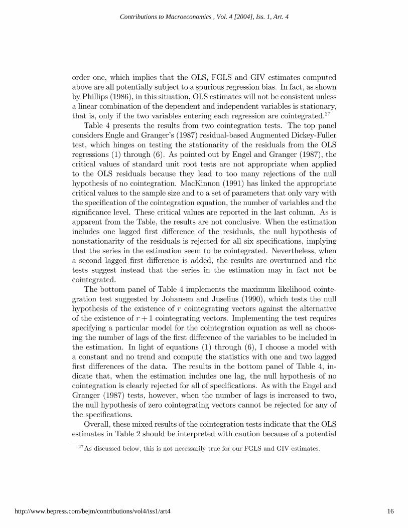
Table 4 presents the results from two cointegration tests. The top panelconsiders Engle and Granger�s (1987) residual-based Augmented Dickey-Fullertest, which hinges on testing the stationarity of the residuals from the OLSregressions (1) through (6). As pointed out by Engel and Granger (1987), thecritical values of standard unit root tests are not appropriate when appliedto the OLS residuals because they lead to too many rejections of the nullhypothesis of no cointegration. MacKinnon (1991) has linked the appropriatecritical values to the sample size and to a set of parameters that only vary withthe speci�cation of the cointegration equation, the number of variables and thesigni�cance level. These critical values are reported in the last column. As isapparent from the Table, the results are not conclusive. When the estimationincludes one lagged �rst di¤erence of the residuals, the null hypothesis ofnonstationarity of the residuals is rejected for all six speci�cations, implyingthat the series in the estimation seem to be cointegrated. Nevertheless, whena second lagged �rst di¤erence is added, the results are overturned and thetests suggest instead that the series in the estimation may in fact not becointegrated.The bottom panel of Table 4 implements the maximum likelihood cointe-

gration test suggested by Johansen and Juselius (1990), which tests the nullhypothesis of the existence of r cointegrating vectors against the alternativeof the existence of r+ 1 cointegrating vectors. Implementing the test requiresspecifying a particular model for the cointegration equation as well as choos-ing the number of lags of the �rst di¤erence of the variables to be included inthe estimation. In light of equations (1) through (6), I choose a model witha constant and no trend and compute the statistics with one and two lagged�rst di¤erences of the data. The results in the bottom panel of Table 4, in-dicate that, when the estimation includes one lag, the null hypothesis of nocointegration is clearly rejected for all of speci�cations. As with the Engel andGranger (1987) tests, however, when the number of lags is increased to two,the null hypothesis of zero cointegrating vectors cannot be rejected for any ofthe speci�cations.Overall, these mixed results of the cointegration tests indicate that the OLS

estimates in Table 2 should be interpreted with caution because of a potential

27As discussed below, this is not necessarily true for our FGLS and GIV estimates.

16



spurious regression bias. As discussed by Hamilton (1994, p. 562), a naturalcure for spurious regressions would be to di¤erence the data before estimatingthe equations. The disadvantage of this approach is that important long-runinformation would be lost and, in particular, the interpretation of our estimatesof �i would become much less transparent. Interestingly, the existence of aunit root in the OLS residuals implies that the FGLS and GIV estimates inTable 2 are asymptotically equivalent to the estimates that would be obtainedwith the di¤erenced data (cf. Blough, 1992, and the discussion in Hamilton,1994, p. 562). This implies that the estimates in columns VI and VII of Table2 are consistent, but it also indicates that these estimates might be neglectingimportant long-run information in the data.

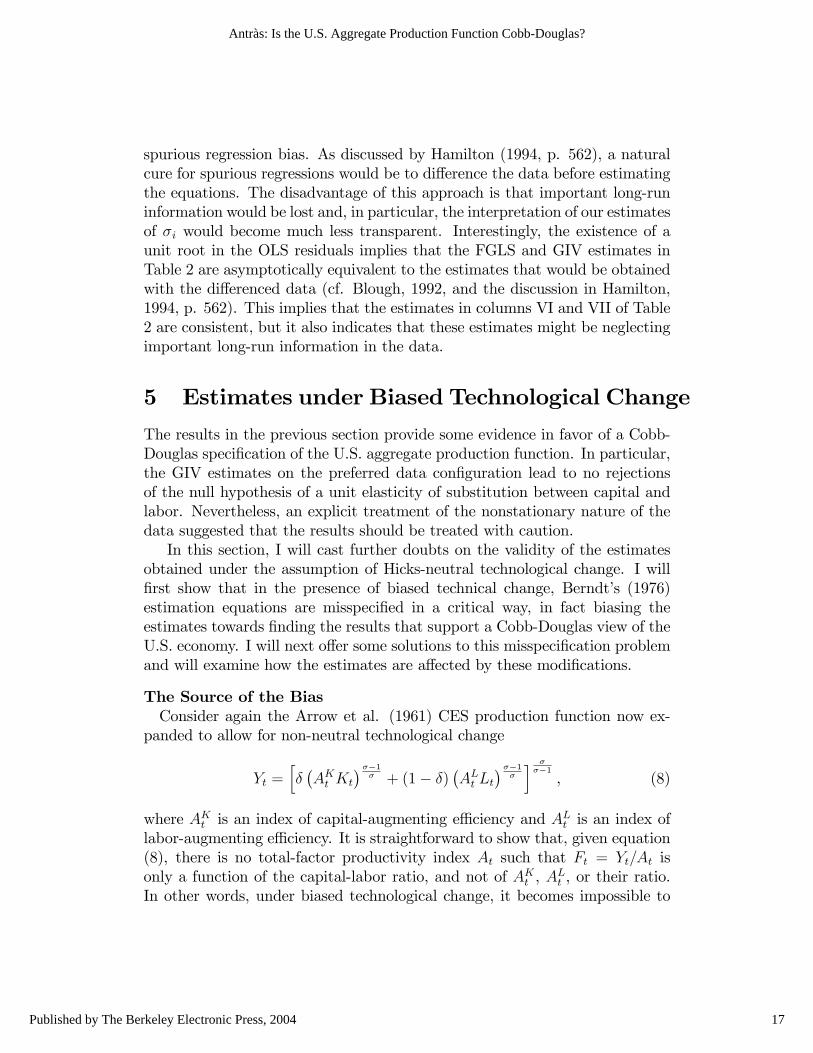
5 Estimates under Biased Technological Change

The results in the previous section provide some evidence in favor of a Cobb-Douglas speci�cation of the U.S. aggregate production function. In particular,the GIV estimates on the preferred data con�guration lead to no rejectionsof the null hypothesis of a unit elasticity of substitution between capital andlabor. Nevertheless, an explicit treatment of the nonstationary nature of thedata suggested that the results should be treated with caution.In this section, I will cast further doubts on the validity of the estimates

obtained under the assumption of Hicks-neutral technological change. I will�rst show that in the presence of biased technical change, Berndt�s (1976)estimation equations are misspeci�ed in a critical way, in fact biasing theestimates towards �nding the results that support a Cobb-Douglas view of theU.S. economy. I will next o¤er some solutions to this misspeci�cation problemand will examine how the estimates are a¤ected by these modi�cations.

The Source of the BiasConsider again the Arrow et al. (1961) CES production function now ex-

panded to allow for non-neutral technological change

Yt =h��AKt Kt

��1� + (1� �)

�ALt Lt

��1�

i ��1, (8)

where AKt is an index of capital-augmenting e¢ ciency and ALt is an index of

labor-augmenting e¢ ciency. It is straightforward to show that, given equation(8), there is no total-factor productivity index At such that Ft = Yt=At isonly a function of the capital-labor ratio, and not of AKt , A

Lt , or their ratio.

In other words, under biased technological change, it becomes impossible to

17



remove factor e¢ ciency from the aggregate input index Ft. This implies that,under these circumstances, the estimations equations (1), (2), (4), and (5),which include Ft and its associated price, are all misspeci�ed in the sense thatthey su¤er from an omitted-variable bias. Furthermore, taking the �rst orderconditions with respect to capital and labor, one can obtain the followingexpression from which equations (3) and (6) are derived:

log

�Wt

Rt

�= log

�1� ��

�+

�1

�

�log

�Kt

Lt

�+

�1� ��

�log

�AKtALt

�(9)

Equation (9) clearly illustrates that as long as AKt 6= ALt (i.e., as long astechnological change is non-neutral) equations (3) and (6) also su¤er from anomitted-variable bias. To get a better understanding on the direction of thebias, it is useful to subtract log (Kt=Lt) from equation (9):

log

�WtLtRtKt

�= log

�1� ��

�+

�1� ��

�log

�AKt Kt

ALt Lt

�. (10)

The left-hand side of equation (10) is simply the logarithm of the labor sharein total output divided by the capital share. As discussed in the introduction,this variable has been remarkably stable over the period 1948-1998. On theother hand, the capital-labor ratio Kt=Lt on the right-hand side of (10) hassteadily increased during the same period. Consequently, whenever the bias intechnological change is ignored, i.e., whenever the ratio AKt =A

Lt is not included

in the regression, the estimate of (1� �) =� will necessarily be close to zero,implying that the estimate of � will necessarily be close to one. At �rstglance this does not seem surprising: if a Cobb-Douglas function describeswell aggregate production in the U.S. private sector, the labor share shouldbe approximately constant. The problem is that in the presence of biasedtechnological change the argument does not run both ways. As it is clearfrom equation (10), if Kt=Lt and ALt =A

Kt grow at the same rate, then steady

factor shares can be consistent with any well-behaved production function,and certainly with aggregate production functions with non-unit elasticities ofsubstitution.A notable example is a version of the neoclassical growth model with labor-

augmenting technological change (cf., Barro and Sala-i-Martin, 1995, Chapter2). With rather weak conditions on the aggregate production function, themodel delivers a balance growth path in which the capital-labor ratio grows atthe same rate as the index of labor-augmenting e¢ ciency. Another exampleis provided by Acemoglu (2003), who develops a model in which the incen-

18



tives to innovate depend on the size of the bill paid to each factor. In hismodel an increase in the labor share encourages labor-augmenting technologi-cal change, which in turn increases the capital-labor ratio and the wage-rentalratio. The fact that capital and labor are assumed to be gross complements(� < 1) ensures that the increase in K=L is higher than the increase in w=r,thereby bringing the labor share back to its steady-state equilibrium value.Acemoglu�s (2003) model nicely illustrates the misspeci�cation inherent in re-stricting technological change to be neutral in the regressions above. By notcontrolling for the bias in technological change, one is implicitly ascribing thefull variation in the capital-labor to factor substitution, when in fact part ofthe variation is explained by technological change.

Model Speci�cation and Additional DataAs discussed above, in the presence of biased technological change, it is

impossible to construct an index of aggregate input Ft that is independentof the e¢ ciency indices AKt and ALt . Consequently, in order to consistentlyestimate the elasticity of substitution, it becomes necessary to device a methodto control for these indices, which in turn requires the imposition of some typeof structure on the form of technological change (cf., Diamond, McFaddenand Rodriguez, 1978). I follow the bulk of the literature in assuming thatAKt and A

Lt grow at constant rates �K and �L.

28 Under this assumption, theproduction function (7) becomes

Yt =h��AK0 e

�K �tKt

��1� + (1� �)

�AL0 e

�L�tLt��1

�

i ��1.

The �rst-order conditions for pro�t maximization can then be manipulated toobtain the following six speci�cations, analogous to equations (1) through (6)in section 2:29

log(Yt=Kt) = �0

1 + � log(Rt=PYt ) + (1� �)�K � t+ "1;t (1�)

log(Yt=Lt) = �0

2 + � log(Wt=PYt ) + (1� �)�L � t+ "2;t (2�)

log(Kt=Lt) = �03 + � log(Wt=Rt) + (1� �)(�L � �K) � t+ "3;t (3�)

log(Rt=PYt ) = �

04 + (1=�) log(Yt=Kt)� [(1� �) =�]�K � t+ "4;t (4�)

log(Wt=PYt ) = �

05 + (1=�) log(Yt=Lt)� [(1� �) =�]�L � t+ "5;t (5�)

28Below, I brie�y discuss an alternative speci�cation with technological change beingpartly stochastic.29Lucas (1969), David and van de Klundert (1965), and Kalt (1978) estimate di¤erent

subsets of these speci�cations.

19



log(Wt=Rt) = �0

6 + (1=�) log(Kt=Lt)� [(1� �) =�] (�L � �K) � t+ "6;t. (6�)

There are two important di¤erences between the speci�cations in (1�) through(6�) and those in (1) through (6). First, because of the impossibility of con-structing an aggregate input index Ft, this index is replaced by real outputYt. Second, all six speci�cations now include a time trend. As is clear fromthe equations, the exclusion of the time trend in the regressions above, wouldin general lead to inconsistent estimates of the elasticity of substitution. Theonly exception is the Cobb-Douglas case (� = 1), in which the bias woulde¤ectively be zero.30

Estimation of equations (1�) through (6�) requires data on real output Ytand its associated price P Yt . A natural candidate to proxy for Yt is real GDPin the U.S. private sector. As argued by Berndt (1976), using value added tomeasure Yt is in general problematic. As he points out, most studies consideronly a subset of capital inputs, namely equipment and structures, thus ignoringland, inventories, and working capital. Because in this paper I have alsofocused on capital equipment and structures, the use of value added as aproxy for Yt is arguably inappropriate. Nevertheless, in the presence of biasedtechnological change, Berndt�s (1976) approach of constructing the aggregateinput index is infeasible, because the index Ft will necessarily depend on AKtand ALt , which are unobservable. Furthermore, as discussed above, ignoringthe adjustment for AKt and A

Lt is not an option, since this leads to estimates

of the elasticity that are necessarily biased towards one. The infeasibility ofusing Berndt�s (1976) aggregate input approach inclines me to use series onvalue added. In particular, I use GDP in the U.S. private sector to proxy forYt, and the corresponding GDP de�ator to proxy for P Yt .

Estimation ResultsColumn I in Table 5 presents OLS estimates of equations (1�) through (6�).

In order to assess the e¤ect of controlling for biased technological change, theseestimates should be compared with those in column V of Table 2. As it is clearfrom the results, the point estimates of the elasticity drop to values that are, ingeneral, well below one and that range from 0:551 to 0:948. Furthermore, thestandard errors of the estimates are quite low, implying that the null hypothesisof a unit elasticity is rejected at the 1% signi�cance level for �ve of the sixspeci�cations, while it is rejected at the 10% level for the remaining equation(see the t-stats in Table 5). Interestingly, the estimates are also consistent withthe empirical regularity discussed in Berndt (1976), by which the estimates of

30Notice also that the constant terms are not only a function of �, but depend also on �,AK0 and AK0 (see Klump and De La Grandville, 2000, for more on this).

20



the elasticity based on the marginal product of labor equations tend to behigher than the estimates based on the marginal product of capital equations.As in the regressions in section 4, the Durbin-Watson statistics indicate theexistence of serial correlation in the residuals.31 I performed again Ljung-Boxtests and the null hypothesis of the residuals following an AR(1) process wasagain not rejected.Column II in Table 5 presents FGLS estimates that apply the Prais-Winsten

procedure. The results are qualitatively similar to the OLS ones, with the low-est estimates becoming even lower and the highest estimate reaching a valueslightly higher than one. Finally, in column III, I present estimates based onFair�s (1970) GIV technique. Instrumentation seems to help a great deal inbringing the estimates from di¤erent speci�cations closer together. In partic-ular, the GIV estimates range from 0:681 to 0:891, and even the highest pointestimate, �5, is signi�cantly lower than one at the 5% signi�cance level. Over-all, of the eighteen estimates in columns I, II, and III, seventeen are below one,with �fteen of these estimates being signi�cantly below one at the 5% level.Furthermore, the typical elasticity lies in the range 0.6 to 0.9.The high R-squares and low Durbin-Watson statistics obtained under OLS

suggest that, as in section 4, the results might su¤er from a spurious regres-sion bias. Section 4 uncovered signi�cant nonstationarities in the data used inthe regressions with Hicks-neutral technological change. I repeated the unitroot tests for the series involved in the estimation of equations (1�) through(6�) and found very similar results. The null hypothesis of the series beingintegrated of order one was not rejected in any of the six cases, while the nullhypothesis of their �rst di¤erence being integrated of order one was clearly re-jected in all cases. These results call for a cointegration test to assess whetheror not the regressions above are spurious. The top panel of Table 6 presentsthe results of Engle and Granger�s (1987) residual-based test. The residualsare obtained from a model that includes a time trend, and the speci�cationof the test includes one, two or three lags of the �rst di¤erence of the resid-uals. The statistics reported in Table 6 should be compared with the criticalvalues computed à la MacKinnon (1991), which are also adjusted to take intoaccount the time trend in the equations. As in section 4, the results are notconclusive. When the estimation includes one lag, the tests generally reject thenull hypothesis of no cointegration, but the results are not robust to adding asecond lagged �rst di¤erence of the residuals. Similarly, in the bottom panelof Table 6 I report the Johansen and Juselius (1990) test, which equally de-

31These statistics are not reported to save space. Even the highest Durbin-Watson statisticwas lower than one.

21



Table 5. Estimates Allowing for Biased Technological Change

OLS FGLS GIV Saikkonen With Lags

I II III IV V

1 �1 0.551 0.407 0.681 0.641 0.408t-stat for H0: �1 = 1 -9.55 -14.2 -3.43 -2.79 -15.07

R2 0.972 0.996 0.905 0.977 0.993

2 �2 0.908 0.918 0.880 0.872 1.004t-stat for H0: �1 = 1 -3.36 -2.02 -3.00 -2.94 0.04

R2 0.998 0.996 0.992 0.999 0.999

3 �3 0.596 0.378 0.685 0.687 0.313t-stat for H0: �1 = 1 -8.33 -11.7 -3.06 -2.27 -15.74

R2 0.992 0.995 0.981 0.994 0.998

4 �4 0.743 0.637 0.770 0.807 0.578t-stat for H0: �1 = 1 -4.05 -5.65 -2.08 -0.70 -7.58

R2 0.933 0.965 0.623 0.940 0.969

5 �5 0.948 1.013 0.891 0.892 1.521t-stat for H0: �1 = 1 -1.84 0.28 -2.70 -1.95 3.20

R2 0.998 0.996 0.994 0.999 0.999

6 �6 0.785 0.750 0.772 0.797 0.587t-stat for H0: �1 = 1 -3.35 -2.59 -1.93 -0.77 -5.03

R2 0.983 0.977 0.896 0.984 0.991

No. of Obs. 51 51 50 48 50

Table 6. Cointegration Tests for Model with a Time Trend

A. Residual-Based Augmented Dickey-Fuller Tests

Residuals Residuals Residuals Residuals Residuals Residuals 5% Criticalof eq. (1) of eq. (2) of eq. (3) of eq. (4) of eq. (5) of eq. (6) Value

ADF 0 -2.407 -4.783 -2.860 -2.990 -4.509 -3.262 -3.501ADF 1 -3.071 -4.165 -3.219 -3.533 -3.948 -3.719 -3.502ADF 2 -2.641 -3.086 -2.315 -2.965 -3.027 -3.006 -3.504

B. Johansen-Juselius Cointegration Tests

Max-Lambda Trace

Test r = 0 vs r = 1 r � 1 vs r = 2 r = 0 vs r = 1 r � 1 vs r = 2Num. of lags 1 2 1 2 1 2 1 2

log(Y=K) & log(r) 26.83 12.97 0.00 5.41 26.83 18.38 0.00 5.41log(Y=L) & log(w) 40.72 17.28 0.12 0.10 40.84 17.38 0.12 0.10log(K=L) & log(w=r) 27.12 9.76 0.05 1.47 27.17 11.23 0.05 1.47

95 % Critical Values 18.96 12.25 25.32 12.25

22



livers di¤erent conclusions depending on the number of lags speci�ed in theestimation. Both types of tests suggest, however, that the null hypothesis ofno cointegration is more easily rejected in the case of the marginal product oflabor equations (2�) and (5�).32

The mixed results of the cointegration tests complicate the evaluation ofthe consistency of the OLS estimates presented in Table 5. On the one hand,if we are willing to reject the null hypothesis of no cointegration (i.e., if webelieve the tests should be speci�ed with one lag), OLS estimates are notonly consistent but also superconsistent, in the sense that they converge totheir true value at a higher speed than in the absence of nonstationarity inthe series (cf., Phillips and Durlauf. 1986, and Stock, 1987). Furthermore,in that case, OLS estimates are consistent even in the presence of autocor-relation in the disturbances and endogeneity of the regressors. Phillips andDurlauf (1986) showed, however, that OLS estimates of cointegrated relation-ships have nonstandard asymptotic distributions, thus invalidating standardinference techniques. Furthermore, small-sample biases, which are likely to beimportant in our regressions, suggest the need to use alternative superior esti-mates. Saikkonen (1991) suggests a simple modi�cation to the OLS procedure,which delivers both consistent and e¢ cient estimates that have asymptoticallystandard distributions.33

On the other hand, if we interpret the results in Table 6 as indicating thatthe null hypothesis of no cointegration cannot be rejected (i.e., if we believethe tests should be speci�ed with two lags), then OLS estimates su¤er froma spurious regression bias, and are therefore inconsistent. As argued before, anatural cure for this bias is to di¤erence the data before estimating the equa-tions, the disadvantage being that, by doing so, valuable long-run informationmay be lost. An alternative approach is to include lagged values of both thedependent and independent variables in the regression. This procedure leadsto consistent estimates of the elasticity and to t-tests of the hypothesis �i = 1that are asymptotically N (0; 1).34

Rather than taking a strong stance on whether the variables in the re-gressions are in fact cointegrated or not, I next report the results of applyingSaikkonen�s (1991) procedure for estimating cointegrating vectors, as well as

32The statistics in the Engle and Granger (1987) are always higher for these two equa-tions. Furthermore, even with two lagged �rst di¤erences in the estimation, the max-lambdastatistic in the Johansen and Juselius test is very close to its critical value for this pair ofvariables.33See King, Plosser, Stock and Watson (1991) for an application of a similar technique.34Conversely, F tests of hypotheses that a set of estimates are jointly signi�cant have

nonstandard limiting distribution (c.f., Hamilton, pp. 562).

23



standard OLS estimates that include lagged values of both variables to correctfor spurious regression bias in the absence of cointegration.35

Column IV of Table 5 presents the results of the implementation of Saikko-nen�s (1991) procedure for l = 1 and p = 1. The details of the estimationprocedure are relegated to Appendix B. For each of the six regressions, thetable reports the estimate of the elasticity of substitution and the modi�edt-statistic, which should be compared with the associated critical value from astandard normal distribution.36 The results indicate that the inclusion of theleads and lags does not have much of an e¤ect on the point estimates of theelasticity, which are very similar to those obtained under the GIV procedurein column III of Table 5. The modi�ed t-statistics are somewhat lower thanthe standard ones, but they still lead to a rejection of the null hypothesis of aunit elasticity (at reasonable signi�cance levels) in four of the six cases.Finally, in column V of Table 5, I report OLS estimates extended to include

lagged values of both the dependent variable yt and the independent variablext, as well as a time trend. This has a larger impact on the estimates, sug-gesting that spurious regression biases might be important. The estimates ofthe elasticity obtained from equations (1�), (3�), (4�), and (6�) are substantiallylower than the ones obtained in the �rst four columns of Table 5, and provideevidence that the elasticity of substitution might well be lower than 0:5. Thesevalues are consistent with the �ndings of David and van de Klundert (1965),Eisner and Nadiri, and Lucas (1969). On the other hand, the estimates of theelasticity obtained from equations (2�) and (5�) indicate that the elasticity ismuch higher, and might even be larger than one. Remember, however, thatthe approach of adding lags of both variables in the model is only appropriateunder the null hypothesis of no cointegration of the variables. The fact thatthis hypothesis was relatively easier to reject for the variables in equations (2�)and (5�) suggests that these high values of the elasticity should not be takenat face value.

Estimates of the Bias in Technological ChangeAs is apparent from equations (1�) through (6�), with the our estimates

of the elasticity of substitution at hand, we can also obtain estimates of theparameters �K and �L, that is, estimates of the growth rate of capital- andlabor-augmenting technological change. This was already recognized by David

35The Saikonnen (1991) procedure also adds lags to the estimated equation (see AppendixB). Although the introduction of these lags is here justi�ed on statistical grounds, these lagscould also be rationalized appealing to adjustment costs in capital and labor (see Lucas,1969).36This modi�ed t-statistic corresponds to t �

ps2=� in Appendix B.

24



and van de Klundert (1965) who ran an equation analogous to (2�) for the U.S.private sector in the period 1899-1960 and found �L = 0:019, or a growth rateof labor e¢ ciency of 1.9 percent a year. They also ran equations analogous to(3�), both with and without lags, thus obtaining values for �L � �K of 0.72%and 0.86% per year, respectively. As shown in Table 6, using my own estimatesof �3 from equation (2�) under Saikonnen�s procedure (i.e., column IV), yieldsan estimate of �L of 1.85% per year, a �gure remarkably close to David andvan de Klundert�s. Furthermore, when computing �L with the estimates of thereverse equation (5�), I obtain a value of 1.90% which matches their �gure tothe second decimal. On the other hand, as is clear from Table 6, my �ndingssuggest that the bias in technological change, �L � �K , is much larger thanthe one they estimated. In particular, I �nd that labor-augmenting e¢ ciencygrew about 3% faster than capital-augmenting e¢ ciency. In fact, my estimatessuggest that capital e¢ ciency shows a downward trend. To understand thisresult, remember that ALt and A

Kt are actually indices of unmeasured quality

or unmeasured e¢ ciency. A possible interpretation of the �ndings on Table 7is that the Krusell et al. (2000) price of capital de�ator does a better job ofincorporating quality improvements than does the Jorgenson and Ho (2000)quality-adjusted labor input index.

Table 7. Estimates of the Bias in Technological Change

Estimate of Coe¢ cient on Implied coe¢ cientElasticity time trend of technological change

Eq. (1�) 0.641 -0.005 �K = �1:34%Eq. (2�) 0.872 0.002 �L = 1:85%Eq. (3�) 0.687 0.010 �L � �K = 3:08%Eq. (4�) 0.807 0.004 �K = �1:56%Eq. (5�) 0.892 -0.002 �L = 1:90%Eq. (6�) 0.797 -0.008 �L � �K = 3:15%

As discussed above, the imposition of a particular structure on the formof technological change is dictated by the need to identify the elasticity ofsubstitution. Given this constraint, the choice of constant exponential growthrates of factor e¢ ciency seems a natural one. Alternatively, one could con-sider a speci�cation that allowed for a stochastic component in technologicale¢ ciency. In particular, consider the case in which AKt = AK0 e

�K �t+�Kt and

25



ALt = AL0 e�L�t+�Lt . It is straightforward to check that the stochastic compo-

nents �Kt and �Lt would enter as disturbance terms in the �rst-order conditions

that form the basis of the empirical speci�cations. In section 2, these errorterms had been justi�ed appealing to optimization errors on the part of �rms.Technological shocks provide a second plausible explanation for these terms.Notice, however, that omitted e¢ ciency shocks are much more likely to becorrelated with factor demands than optimization errors are. The reason isthat although �Kt and �

Lt are unobserved by the econometrician, they may be

in the information set of �rms, which will take them into account in choosinginput demands. This suggests that, to the extent that �rms respond quicklyto productivity shocks, my estimates of the elasticity might be biased. Re-member, however, that the generalized instrumental variable (GIV) estimatesin Table 5 (column III) are remarkably close to those obtained under Saikko-nen�s (1991) method. To the extent that the instruments used in the GIVestimation (U.S. population, wages in the government sector, and real capitalstock owned by the government) are unresponsive to technology shocks butare correlated with the variables in equations (1�) through (6�), the results inTable 5 indicate that ruling out stochastic components in AKt and A

Lt does not

have a sizeable e¤ect on the estimates of the elasticity.37

6 Conclusion

This paper has argued that a Cobb-Douglas speci�cation of the U.S. aggregateproduction function may be misleading. My estimates suggest that, controllingfor biased technological change, the elasticity of substitution between capitaland labor is likely to be considerably below one, and may even be lower than0.5. This contrasts with the results of Berndt (1976), who reported estimatesof the elasticity insigni�cantly di¤erent from one under the assumption ofHicks-neutral technological change. I have shown, however, that ignoring thebias in technological change puts the data in a straightjacket that naturallyleads to an acceptance of the null hypothesis of a unit elasticity of substitutionbetween capital and labor. I illustrated this source of bias by showing that, inmy sample, ignoring biased technological change also leads to estimates of theelasticity insigni�cantly di¤erent from one.

37I have also experimented with an alternative speci�cation of AKt and ALt that allowsfor di¤erent growth rates of factor-bias in di¤erent subperiods. This amounts to includingdummy variables for di¤erent subperiods, e.g., 1948-1960, 1961-1972, 1973-1984, 1985-1998.This leads to slightly lower estimates of the elasticity for most speci�cations and estimationtechniques, but the results are very similar to those reported in Table 5.

26



The results are relevant for the debates on the sources of economic growth,as well as for the debate on the e¤ects of tax behavior on investment. Hsieh(2000) shows that when the elasticity of substitution between capital and laboris lower than one, standard growth accounting exercises tend to understate therole of productivity growth as a determinant of economic growth. Similarly, aspointed out by Eisner and Nadiri (1968), low values of the elasticity of substi-tution imply e¤ects of tax policy on investment behavior that are signi�cantlylower than the ones advocated by Hall and Jorgenson (1967), who consideredonly the Cobb-Douglas case.Although the analysis has been conducted with only U.S. data, the �nd-

ings of this paper lend support to a recent literature that has pushed the viewthat certain cross-country stylized patterns are not reconcileable with aggre-gate output being represented by an aggregate production function featuringa unit elasticity of substitution (e.g.,. Acemoglu, 2002, Caselli and Coleman,2003, and Jones, 2003). Consistent with my �ndings, Gollin (2002) shows thateven after adjusting labor income to include self-employment income, employeecompensation as a share of GDP di¤ers substantially across countries. Fur-thermore, other studies have documented large movements of the labor sharein OECD countries and have related these movements to the capital-labor ra-tio (e.g., Blanchard, 1997 and Bentolila and Saint-Paul, 2003). My estimatessuggest that even for a country, the United States, with a relatively stablelabor share, the evidence seems to reject a Cob-Douglas speci�cation of theaggregate production function.

27



Colophon

Acknowledgments: I am grateful to Daron Acemoglu, Lucia Breierova,Robert Chirinko, Jerry Hausman, Rainer Klump, two anonymous referees andthe Editor (Chad Jones) for very helpful comments, and to David Romer forencouraging me to pursue this project. Financial support from the Bank ofSpain is gratefully aknowledged. All remaining errors are my own.Email: [email protected]: Department of Economics, Harvard University, Littauer

230, Cambridge, MA 02138.

Appendix A

This Appendix discusses Fair�s (1970) GIV procedure. The model I considercan be summarized by the following two equations:

yt = �+ �xt + "t ; t = 1; :::; T

"t = �"t�1 + ut ; t = 1; :::; T ,

where E ["tjxt] 6= 0, but there exists a vector of instrumental variables Z thatsatis�es plim 1

TZ 0txt 6= 0 and plim 1

TZ 0t"t = 0. Fair (1970) showed that this

type of model could be estimated consistently and e¢ ciently by the followingthree-step procedure:38

1. First, project xt on the set of instruments Z and compute the �ttedvalues bxt = Zt(Z

0tZt)

�1Z0txt. Estimate the equation yt = � + �bxt + �t, thus

obtaining consistent estimates e� and e�.2. Letting b"t = yt � e� � e�xt, obtain an estimate b� in a regression of b"t onb"t�1.3. Estimate the equation yt�b�yt�1 = (bxt � b�xt�1) �+ut and obtain b�, the

�nal estimate.The only additional requirement needed to achieve consistency is to include

the lagged values of both Y and X in the set of instruments. Fair also showedthat an asymptotically consistent estimate of the variance of b� is given by

Est:V ar[b�] = 1T

PTt=2

�yt � b�yt�1 � (xt � b�xt�1) b��2PT

t=2 (wt � w)2

38Fair�s (1970) procedure is in fact much more general than the simpli�ed example pre-sented here.

28



where wt = bxt � b�xt�1.Appendix B

This Appendix discusses Saikonnen�s (1991) two-step procedure. If the initialmodel is

yt = �+ �xt + �t+ "t,

Saikkonen�s (1991) two-step procedure �rst involves adding leads and lagsof the �rst di¤erence of the independent variable to this equation, and thenmodifying the standard error of the estimate of � making use of the estimatedresiduals, whose stochastic process is approximated by an AR(p) process. Morespeci�cally, the procedure can be summarized as follows:

1. Run yt = �+ �xt + �t+Pl

s=�l l�xt�l + ut, compute but and constructs2 =

Pt bu2t= (T �K), where K is the number of regressors including the

constant.

2. Run but = �1but�1 + �2but�2 + :::+ �pbut�p + �t and construct� =

1

T � p

PTt=p+1 b�2t

1� b�1 � :::� b�p!.

Saikkonen (1991) showed that the estimate of � obtained in step 1 is bothconsistent and asymptotically e¢ cient. More importantly, if t is the t-statisticcorresponding to a test on the estimate of �, Saikkonen (1991) proved that:39

t �ps2

�

d! N(0; 1):

39Stock and Watson (1993) also proved that this procedure yields estimates that are as-ymptotically equivalent to those obtained with Johansen�s (1988, 1991) Gaussian MaximumLikelihood technique.

29



References

Acemoglu, Daron K. (2002), �Directed Technical Change,�Review of Eco-nomic Studies, 69, pp. 781-810.

Acemoglu, Daron K. (2003), �Labor- and Capital-Augmenting TechnicalChange,�Journal of the European Economic Association, 1, pp. 1-37.

Antràs, Pol (2003), �Is the U.S. Aggregate Production Function Cobb-Douglas?New Estimates of the Elasticity of Substitution,� Harvard University,mimeo.

Arrow, Kenneth J., Hollis B. Chenery, Bagicha Minhas, and Robert M. Solow(1961), �Capital-Labor Substitution and Economic E¢ ciency,�Reviewof Economics and Statistics, 43:5, pp. 225-254.

Barro, Robert, and Xavier Sala-i-Martin (1995), Economic Growth, Cam-bridge, MA: MIT Press.

Basu, Susanto (1996), �Procyclical Productivity: Increasing Returns or Cycli-cal Utilization?,�Quarterly Journal of Economics, 111:3, pp. 719-751.

Bentolila, Samuel, and Gilles Saint-Paul (2003), �Explaining Movementsin the Labor Share�, Contributions to Macroeconomics, 3:1, Article 9,http://www.bepress.com/ bejm/contributions/vol3/iss1/art9.

Berndt, Ernst (1976), �Reconciling Alternative Estimates of the Elasticity ofSubstitution,�Review of Economics and Statistics, 58:1, pp. 59-68.

(1991), The Practice of Econometrics: Classic and Contemporary.Reading, Mass.: Addison-Wesley.

and Laurits R. Christensen (1973), �The Translog Function and theSubstitution of Equipment, Structures and Labor in U.S. Manufacturing1929-68,�Journal of Econometrics, March, pp. 81-114.

Blanchard, Olivier (1997), �The Medium Run,�Brookings Papers on Eco-nomic Activity, pp. 89-158.

Blough, Stephen R. (1992), �Spurious Regressions, with AR(1) Correctionand Unit Root Pretest,�Johns Hopkins University, Mimeo.

30



Bound, John, David A. Jaeger and Regina M. Baker (1995), �Problems withInstrumental Variables Estimation When the Correlation Between theInstruments and the Endogeneous Explanatory Variable is Weak,�Jour-nal of the American Statistical Association, 90:430, pp. 443-450.

Burnside, Craig, Martin Eichenbaum, and Sergio Rebelo (1995), �CapitalUtilization and Returns to Scale,�NBER Macroeconomics Annual 1995,pp. 67-110.

Chirinko, Robert S. (2002), �Corporate Taxation, Capital Formation, andthe Substitution Elasticity between Capital and Labor,�National TaxJournal, 55:2, pp. 339-355.

Coen, R. M. (1969), �Tax Policy and Investment Behavior: A Comment,�American Economic Review, 59:3, pp. 370-379.

David, Paul A. and Th. van de Klundert (1965), �Biased E¢ ciency Growthand Capital-Labor Substitution in the U.S., 1899-1960,�American Eco-nomic Review, 55, pp. 357-393.

Dhrymes, P. J., and P. Zarembka (1970), �Elasticities of Substitution forfor Two-Digit Manufacturing Industries: A Correction,�Review of Eco-nomics and Statistics, February, pp. 115-117.

Diamond, Peter, Daniel McFadden, and Miguel Rodriguez (1978), �Mea-surement of the Elasticity of Factor Substitution and Bias of TechnicalChange,� in Production Economics: A Dual Approach to Theory andApplications (Volume 2), edited by Melvyn Fuss and Daniel McFadden,Amsterdam: North-Holland, pp. 125-147.

Diewert, W. Erwin (1971), �An Application of the Shepard Duality Theo-rem: A Generalized Linear Production Function,� Journal of PoliticalEconomy, 79:3, pp. 482-50.

Eisner, R., and M. I. Nadiri (1968), �Investment Behavior and the Neoclas-sical Theory,�Review of Economics and Statistics, 50:3, pp. 369-382.

Engle, Robert F. and Clive W. J. Granger (1987), �Co-Integration and ErrorCorrection: Representation, Estimation, and Testing,� Econometrica,55:2, pp. 251-276.

Gollin, Douglas (2002), �Getting Income Shares Right,�Journal of PoliticalEconomy, 110:2, pp. 458-474.

31



Gordon, R. J. (1990), The Measurement of Durable Goods Prices, NationalBureau of Economic Research Monograph Series, Chicago: University ofChicago Series.

Granger, Clive W. J. and Paul Newbold (1974), �Spurious regressions ineconometrics,�Journal of Econometrics, 2, pp. 111-120.

Greene, William H. (1999), Econometric Analysis, fourth edition, New York:MacMillan.

Fair, Ray C. (1970), �The Estimation of Simultaneous Equation Models withLagged Endogenous Variables and First Order Serially Correlated Er-rors,�Econometrica, 38:3, pp. 507-516.

Fraumeni, Barbara M. (1997), �The Measurement of Depreciation in theNIPA�s,�Survey of Current Business, July, Bureau of Economic Activity.

Hall, Robert E. and Dale W. Jorgenson (1967), �Tax Policy and InvestmentBehaviour�, American Economic Review, 57, pp. 391- 414.

Hamilton, James (1994), Time Series Analysis, Princeton, NJ: PrincetonUniversity Press.

Hausman, Jerry A. (1978), �Speci�cation Tests in Econometrics,�Economet-rica, 46:6, pp. 1251-1271.

(1983), �Speci�cation and Estimation of Simultaneous Models,�inZ. Griliches and M. Intriligator (eds.), Handbook of Econometrics, Vol.1, 1983, pp. 391-448.

Herman, Shelby W. (2000), �Fixed Assets and Consumer Durable Goods�Estimates for 1925-98 and New NIPA Table: Changes in Net Stock ofProduced Assets,� Survey of Current Business, April, Bureau of Eco-nomic Activity.

Hsieh, Chang-Tai (2000), �Measuring Biased Technological Change,�Prince-ton University, mimeo.

Johansen, Soren (1988), �Statistical Analysis of Cointegration Vectors,�Jour-nal of Economic Dynamics and Control, 12, pp. 231-54.

(1991), �Estimation and Hypothesis Testing of Cointegration Vec-tors in Gaussian Vector Autoregressive Models,�Econometrica, 59:6, pp.1551-1580.

32



and Katarina Juselius (1990), �Maximum Likelihood Estimationand Inference on Cointegration - With Applications to the Demand forMoney,�Oxford Bulletin of Economics and Statistics, 52, pp. 169-210.

Jones, Charles I. (2003), �Growth, Capital Shares, and a New Perspective onProduction Functions,�University of California at Berkeley, mimeo.

Jorgenson, Dale W. and Mun S. Ho (2000), �The Quality of the U.S. Work-force 1948-95,� Harvard University, mimeo with data update through1999.

and Kevin J. Stiroh (2000), �Raising the Speed Limit: U.S. Eco-nomic Growth in the Information Age,�Brookings Papers on EconomicActivity, 1, pp. 125-211.

Judd, Kenneth L. (1987), �The Welfare Cost of Factor Taxation in a Perfect-Foresight Model," Journal of Political Economy, 95:4, pp. 675-709.

Kalt, Joseph P. (1978), �Technological Change and Factor Substitution in theUnited States: 1929-1967,�International Economic Review, 19, pp.761-775.

King, Robert G., Charles I. Plosser, James H. Stock and Mark W. Wat-son (1991), �Stochastic Trends and Economic Fluctuations,�AmericanEconomic Review, 81:4, pp. 819-840.

Klump, Rainer and Olivier De La Grandville (2000), �Economic Growth andthe Elasticity of Substitution: Two Theorems and Some Suggestions,�American Economic Review, 90:1, pp. 282-291.

Krueger, Alan B. (1999), �Measuring Labor�s Share,�American EconomicReview, 89:2, pp. 45-51.

Krusell, Per, Lee Ohanian, Jose Victor Rios-Rull and Gianluca Violante(2000), �Capital-Skill Complementarity and Inequality: A Macroeco-nomic Analysis�, Econometrica, 68, pp. 1029-1054.

Lucas, Robert E. (1969), �Labor-Capital Substitution in U.S. Manufactur-ing,� in The Taxation of Income from Capital, edited by Arnold Har-berger and Martin J. Bailey, Washington, DC: The Brookings Institu-tion, pp. 223-274.

33



MacKinnon, J. (1991), �Critical Values for Co-Integration Tests,� in R.F.Engle and C.W.J. Granger (eds.) Long-Run Economic Relationships,Oxford University Press, pp. 267-76.

Maddala, G. S. (1965), �Di¤erential Industry E¤ects and Di¤erential FactorE¤ects of Technological Change,�Memo 36, Research Center in Eco-nomic Growth, Stanford University.

Mankiw, Gregory N., David Romer, David N. Weil (1992), �A Contributionto the Empirics of Economic Growth,�Quarterly Journal of Economics,107:2, pp. 407-437.

Nerlove, Marc (1963), �Returns to Scale in Electricity Supply,�in Carl Christ,ed., Measurement in Economics: Studies in Mathematical Economicsand Econometrics in Memory of Yehuda Grunfeld, Standford, CA: Stan-ford University Press, pp. 167-198.

(1967), �Recent Empirical Studies of the CES and Related Produc-tion Functions.�In M. Brown, editor, The Theory and Empirical Analy-sis of Production, New York: Columbia University Press for Studies inIncome and Wealth Series 32, pp. 55-122.

Phillips, Peter C. B. (1986), �Understanding Spurious Regressions in Econo-metrics,�Journal of Econometrics, 33, pp. 311-40.

and Stephen Durlauf (1986), �Multiple Time Series Regression withIntegrated Processes,�Review of Economic Studies, 53:4, pp. 473-495.

Saikkonen, Pentti (1991), �Asymptotically E¢ cient Estimation of Cointegra-tion Regressions,�Econometric Theory, 7, pp. 1-21.

Stock, James H. (1987), �Asymptotic Properties of Least Squares Estimatorsof Cointegrating Vectors,�Econometrica, 55:5, pp. 1035-1056.

Trostel, Philip A. (1993), �The E¤ect of Taxation on Human Capital,�Jour-nal of Political Economy, 101:2, pp. 327-350.

34



Documents

Is the U.S. Aggregate Production Function Cobb-Douglas ... · Is the U.S. Aggregate Production Function Cobb-Douglas? New ... of long-run growth in the absence of ... that deliver