Is the Sample Good Enough? Comparing Data from Twitter’s Streaming API withTwitter’s Firehose

Fred MorstatterArizona State University

699 S. Mill Ave.Tempe, AZ, 85281

Jurgen PfefferCarnegie Mellon University

5000 Forbes Ave.Pittsburgh, PA, 15213

Huan LiuArizona State University

699 S. Mill Ave.Tempe, AZ, 85281

Kathleen M. CarleyCarnegie Mellon University

5000 Forbes Ave.Pittsburgh, PA, 15213

Abstract

Twitter is a social media giant famous for the exchangeof short, 140-character messages called “tweets”. In thescientific community, the microblogging site is knownfor openness in sharing its data. It provides a glanceinto its millions of users and billions of tweets through a“Streaming API” which provides a sample of all tweetsmatching some parameters preset by the API user. TheAPI service has been used by many researchers, compa-nies, and governmental institutions that want to extractknowledge in accordance with a diverse array of ques-tions pertaining to social media. The essential drawbackof the Twitter API is the lack of documentation concern-ing what and how much data users get. This leads re-searchers to question whether the sampled data is a validrepresentation of the overall activity on Twitter. In thiswork we embark on answering this question by compar-ing data collected using Twitter’s sampled API servicewith data collected using the full, albeit costly, Firehosestream that includes every single published tweet. Wecompare both datasets using common statistical metricsas well as metrics that allow us to compare topics, net-works, and locations of tweets. The results of our workwill help researchers and practitioners understand theimplications of using the Streaming API.

IntroductionTwitter is a microblogging site where users exchange short,140-character messages called “tweets”. Ranking as the 10thmost popular site in the world by the Alexa rank in Januaryof 20131, the site boasts 500 million registered users pub-lishing 400 million tweets per day. Twitter’s platform forrapid communication is said to be a vital communicationplatform in recent events including Hurricane Sandy2, theArab Spring of 2011 (Campbell 2011), and several politicalcampaigns (Tumasjan et al. 2010; Gayo-Avello, Metaxas,and Mustafaraj 2011). As a result, Twitter’s data has beencoveted by both computer and social scientists to better un-derstand human behavior and dynamics.

Copyright c© 2013, Association for the Advancement of ArtificialIntelligence (www.aaai.org). All rights reserved.

1http://www.alexa.com/topsites2http://www.nytimes.com/interactive/2012/10/28/nyregion/hurricane-

sandy.html

Social media data is often difficult to obtain, with most so-cial media sites restricting access to their data. Twitter’s poli-cies lie opposite to this. The “Twitter Streaming API”3 is acapability provided by Twitter that allows anyone to retrieveat most a 1% sample of all the data by providing some pa-rameters. According to the documentation, the sample willreturn at most 1% of all the tweets produced on Twitter at agiven time. Once the number of tweets matching the givenparameters eclipses 1% of all the tweets on Twitter, Twit-ter will begin to sample the data returned to the user. Themethods that Twitter employs to sample this data is currentlyunknown. The Streaming API takes three parameters: key-words (words, phrases, or hashtags), geographical boundaryboxes, and user ID.

One way to overcome the 1% limitation is to use the Twit-ter Firehose—a feed provided by Twitter that allows accessto 100% of all public tweets. A very substantial drawback ofthe Firehose data is the restrictive cost. Another drawback isthe sheer amount of resources required to retain the Firehosedata (servers, network availability, and disk space). Conse-quently, researchers as well as decision makers in compa-nies and government institutions are forced to decide be-tween two versions of the API: the freely-available but lim-ited Streaming, and the very expensive but comprehensiveFirehose version. To the best of our knowledge, no researchhas been done to assist those researchers and decision mak-ers by answering the following: How does the use of theStreaming API affect common measures and metrics per-formed on the data? In this article we answer this questionfrom different perspectives.

We begin the analysis by employing classic statisticalmeasures commonly used to compare two sets of data.Based on unique characteristics of tweets, we design andconduct additional comparative analysis. By extracting top-ics using a frequently used algorithm, we compare how top-ics differ between the two datasets. As tweets are linkeddata, we perform network measures of the two datasets. Be-cause tweets can be geo-tagged, we compare the geograph-ical distribution of geolocated tweets to better understandhow sampling affects aggregated geographic information.

3https://dev.twitter.com/docs/streaming-apis

(a) Firehose (b) Streaming API

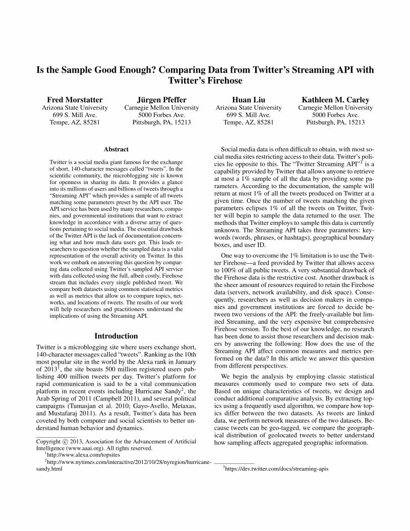
Figure 1: Tag cloud of top terms from each dataset.

Related WorkTwitter’s Streaming API has been used throughout the do-main of social media and network analysis to generate un-derstanding of how users behave on these platforms. It hasbeen used to collect data for topic modeling (Hong and Davi-son 2010; Pozdnoukhov and Kaiser 2011), network analy-sis (Sofean and Smith 2012), and statistical analysis of con-tent (Mathioudakis and Koudas 2010), among others. Re-searchers’ reliance upon this data source is significant, andthese examples only provide a cursory glance at the tip ofthe iceberg. Due to the widespread use of Twitter’s Stream-ing API in various scientific fields, it is important that weunderstand how using a sub-sample of the data generatedaffects these results.

From a statistical point of view, the “law of large num-bers” (mean of a sample converges to the mean of the en-tire population) and the Glivenko-Cantelli theorem (the un-known distribution X of an attribute in a population can beapproximated with the observed distribution x) guaranteesatisfactory results from sampled data when the randomlyselected sub-sample is big enough. From network algorith-mic (Wasserman and Faust 1994) perspective the questionis more complicated. Previous efforts have delved into thetopic of network sampling and how working with a restrictedset of data can affect common network measures. The prob-lem was studied earlier in (Granovetter 1976), where the au-thor proposes an algorithm to sample networks in a way thatallows one to estimate basic network properties. More re-cently, (Costenbader and Valente 2003) and (Borgatti, Car-ley, and Krackhardt 2006) have studied the affect of dataerror on common network centrality measures by randomlydeleting and adding nodes and edges. The authors discoverthat centrality measures are usually most resilient on densenetworks. In (Kossinets 2006), the authors study globalproperties of simulated random graphs to better understanddata error in social networks. (Leskovec and Faloutsos 2006)

proposes a strategy for sampling large graphs to preservenetwork measures.

In this work we compare the datasets by analyzing facetscommonly used in the literature. We start by comparing thetop hashtags found in the tweets, a feature of the text com-monly used for analysis. In (Tsur and Rappoport 2012), theauthors try to predict the magnitude of the number of tweetsmentioning a particular hashtag. Using a regression modeltrained with features extracted from the text, the authors findthat the content of the idea behind the tag is vital to the countof the tweets employing it. Tweeting a hashtag automaticallyadds a tweet to a page showing tweets published by othertweeters containing that hashtag. In (Yang et al. 2012), theauthors find that this communal property of hashtags alongwith the meaning of the tag itself drive the adoption of hash-tags on Twitter. (De Choudhury et al. 2010) studies the prop-agation patterns of URLs on sampled Twitter data.

Topic analysis can also be used to better understand thecontent of tweets. (Kireyev, Palen, and Anderson 2009)drills the problem down to disaster-related tweets, discover-ing two main types of topics: informational and emotional.Finally, (Yin et al. 2011; Hong et al. 2012; Pozdnoukhovand Kaiser 2011) all study the problem of identifying topicsin geographical Twitter datasets, proposing models to ex-tract topics relevant to different geographical areas in thedata. (Joseph, Tan, and Carley 2012) studies how the topicsusers discuss drive their geolocation.

Geolocation has become a prominent area in the study ofsocial media data. In (Wakamiya, Lee, and Sumiya 2011)the authors try to classify towns based upon the contentof the geotagged tweets that originate from within thetown. (De Longueville, Smith, and Luraschi 2009) studiesTwitter’s use as a sensor for disaster information by study-ing the geographical properties of users tweets. The authorsdiscover that Twitter’s information is accurate in the laterstages of a crisis for information dissemination and retrieval.

12

-14

12

-15

12

-16

12

-17

12

-18

12

-19

12

-20

12

-21

12

-22

12

-23

12

-24

12

-25

12

-26

12

-27

12

-28

12

-29

12

-30

12

-31

01

-01

01

-02

01

-03

01

-04

01

-05

01

-06

01

-07

01

-08

01

-09

01

-100

10000

20000

30000

40000

50000

60000

70000

80000

90000N

o.

Tw

eets

Dataset Tweets per Day

StreamingFirehose

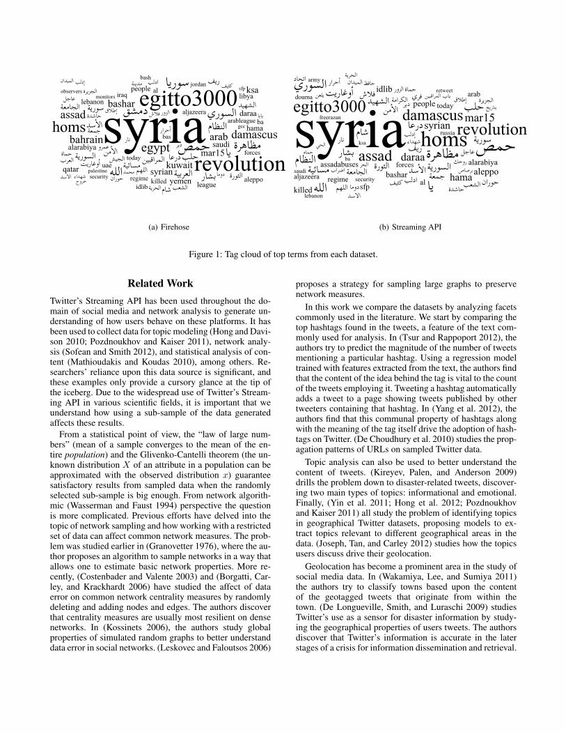
Figure 2: Raw tweet counts for each day from both theStreaming API and the Firehose.

The DataFrom December 14th, 2011 - January 10th, 2012 we col-lected tweets from the Twitter Firehose matching any of thekeywords, geographical bounding boxes, and users in Ta-ble 1. During the same time period, we collected tweetsfrom the Streaming API using TweetTracker (Kumar et al.2011) with exactly the same parameters. During the timewe collected 528,592 tweets from the Streaming API and1,280,344 tweets from the Firehose. The raw counts oftweets we received each day from both sources are shown inFigure 2. One of the more interesting results in this datasetis that as the data in the Firehose spikes, the Streaming APIcoverage is reduced. One possible explanation for this phe-nomenon could be that due to the Western holidays observedat this time, activity on Twitter may have reduced causingthe 1% threshold to go down.

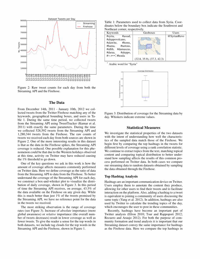
One of the key questions we ask in this work is how theamount of coverage affects measures commonly performedon Twitter data. Here we define coverage as the ratio of datafrom the Streaming API to data from the Firehose. To betterunderstand the coverage of the Streaming API for each day,we construct a box-and-whisker plot to visualize the distri-bution of daily coverage, shown in Figure 3. In this periodof time the Streaming API receives, on average, 43.5% ofthe data available on the Firehose on any given day. Whilethis is much better than just 1% of the tweets promised bythe Streaming API, we have no reference point for the datain the tweets we received.

The most striking observation is the range of coveragerates (see Figure 3). Increase of absolute importance (moreglobal awareness) or relative importance (the overall num-ber of tweets decreases) result in lower coverage as well asfewer tweets. To give the reader a sense for the top words inboth datasets, we include tag clouds for the top words in theStreaming API and the Firehose, shown in Figure 1.

Table 1: Parameters used to collect data from Syria. Coor-dinates below the boundary box indicate the Southwest andNortheast corner, respectively.

Keywords Geoboxes Users#syria, #assad,#aleppovolcano,#alawite, #homs,#hama, #tartous,#idlib, #damascus,#daraa, #aleppo,# *, #houla

@SyrianRevo

(32.8, 35.9), (37.3, 42.3)* Arabic word for “Syria”

0.0

0.2

0.4

0.6

0.8

1.0

Covera

ge o

f Str

eam

ing D

ata

Coverage Distribution

Figure 3: Distribution of coverage for the Streaming data byday. Whiskers indicate extreme values.

Statistical MeasuresWe investigate the statistical properties of the two datasetswith the intent of understanding how well the characteris-tics of the sampled data match those of the Firehose. Webegin first by comparing the top hashtags in the tweets fordifferent levels of coverage using a rank correlation statistic.We continue to extract topics from the text, matching topicalcontent and comparing topical distribution to better under-stand how sampling affects the results of this common pro-cess performed on Twitter data. In both cases we compareour streaming data to random datasets obtained by samplingthe data obtained through the Firehose.

Top Hashtag AnalysisHashtags are an important communication device on Twitter.Users employ them to annotate the content they produce,allowing for other users to find their tweets and to facilitateinteraction on the platform. Also, adding a hashtag to a tweetis equivalent to joining a community of users discussing thesame topic (Yang et al. 2012). In addition, hashtags are alsoused by Twitter to calculate the trending topics of the day,which encourages the user to post in these communities.

Recently, hashtags have become an important part ofTwitter analysis (Efron 2010; Tsur and Rappoport 2012;Recuero and Araujo 2012). For both the purpose of com-munity formation and trend analysis it is important that ourStreaming dataset convey the same importance for hashtagsas the Firehose data. Here we compare the top hashtags in

0 200 400 600 800 1000n

0.4

0.2

0.0

0.2

0.4

0.6

0.8

1.0ta

uTop Hashtags - Firehose and Streaming API

MinQ1MedianQ3Max

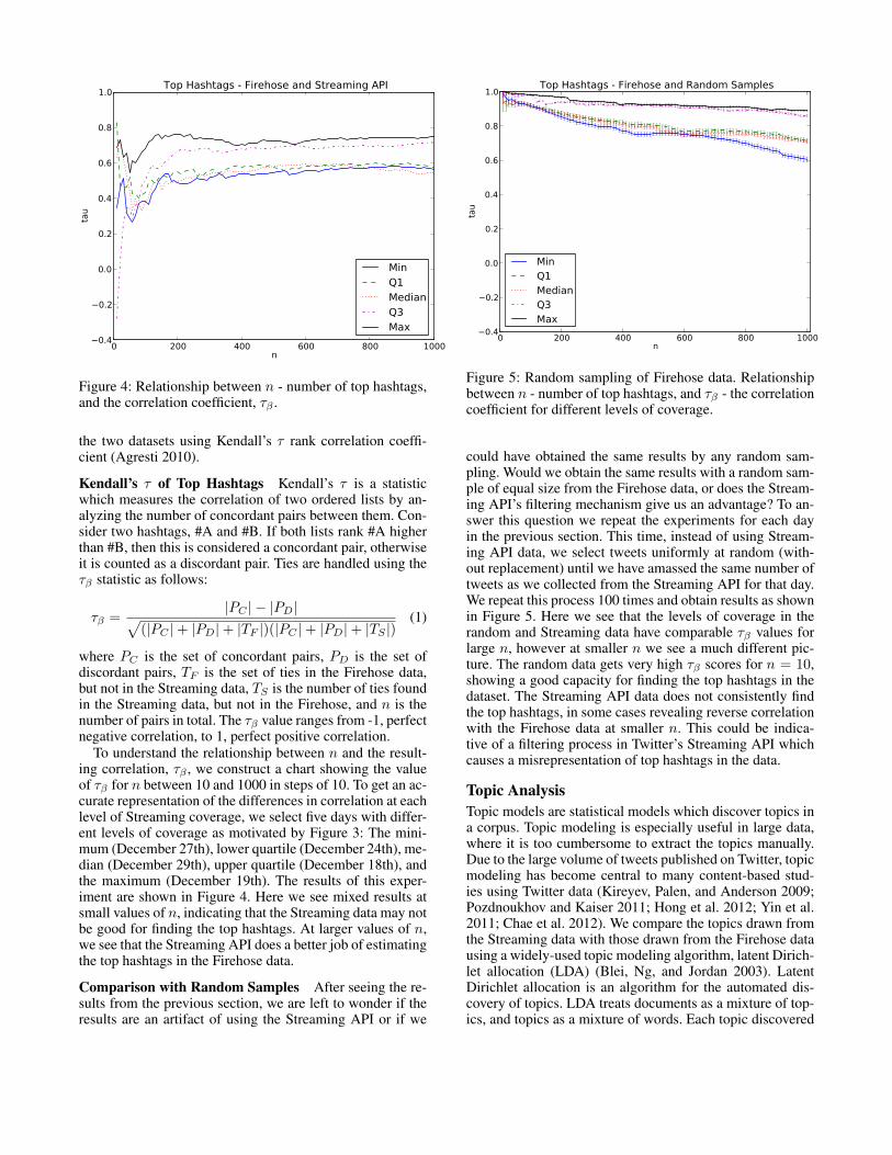
Figure 4: Relationship between n - number of top hashtags,and the correlation coefficient, τβ .

the two datasets using Kendall’s τ rank correlation coeffi-cient (Agresti 2010).

Kendall’s τ of Top Hashtags Kendall’s τ is a statisticwhich measures the correlation of two ordered lists by an-alyzing the number of concordant pairs between them. Con-sider two hashtags, #A and #B. If both lists rank #A higherthan #B, then this is considered a concordant pair, otherwiseit is counted as a discordant pair. Ties are handled using theτβ statistic as follows:

τβ =|PC | − |PD|√

(|PC |+ |PD|+ |TF |)(|PC |+ |PD|+ |TS |)(1)

where PC is the set of concordant pairs, PD is the set ofdiscordant pairs, TF is the set of ties in the Firehose data,but not in the Streaming data, TS is the number of ties foundin the Streaming data, but not in the Firehose, and n is thenumber of pairs in total. The τβ value ranges from -1, perfectnegative correlation, to 1, perfect positive correlation.

To understand the relationship between n and the result-ing correlation, τβ , we construct a chart showing the valueof τβ for n between 10 and 1000 in steps of 10. To get an ac-curate representation of the differences in correlation at eachlevel of Streaming coverage, we select five days with differ-ent levels of coverage as motivated by Figure 3: The mini-mum (December 27th), lower quartile (December 24th), me-dian (December 29th), upper quartile (December 18th), andthe maximum (December 19th). The results of this exper-iment are shown in Figure 4. Here we see mixed results atsmall values of n, indicating that the Streaming data may notbe good for finding the top hashtags. At larger values of n,we see that the Streaming API does a better job of estimatingthe top hashtags in the Firehose data.

Comparison with Random Samples After seeing the re-sults from the previous section, we are left to wonder if theresults are an artifact of using the Streaming API or if we

0 200 400 600 800 1000n

0.4

0.2

0.0

0.2

0.4

0.6

0.8

1.0

tau

Top Hashtags - Firehose and Random Samples

MinQ1MedianQ3Max

Figure 5: Random sampling of Firehose data. Relationshipbetween n - number of top hashtags, and τβ - the correlationcoefficient for different levels of coverage.

could have obtained the same results by any random sam-pling. Would we obtain the same results with a random sam-ple of equal size from the Firehose data, or does the Stream-ing API’s filtering mechanism give us an advantage? To an-swer this question we repeat the experiments for each dayin the previous section. This time, instead of using Stream-ing API data, we select tweets uniformly at random (with-out replacement) until we have amassed the same number oftweets as we collected from the Streaming API for that day.We repeat this process 100 times and obtain results as shownin Figure 5. Here we see that the levels of coverage in therandom and Streaming data have comparable τβ values forlarge n, however at smaller n we see a much different pic-ture. The random data gets very high τβ scores for n = 10,showing a good capacity for finding the top hashtags in thedataset. The Streaming API data does not consistently findthe top hashtags, in some cases revealing reverse correlationwith the Firehose data at smaller n. This could be indica-tive of a filtering process in Twitter’s Streaming API whichcauses a misrepresentation of top hashtags in the data.

Topic AnalysisTopic models are statistical models which discover topics ina corpus. Topic modeling is especially useful in large data,where it is too cumbersome to extract the topics manually.Due to the large volume of tweets published on Twitter, topicmodeling has become central to many content-based stud-ies using Twitter data (Kireyev, Palen, and Anderson 2009;Pozdnoukhov and Kaiser 2011; Hong et al. 2012; Yin et al.2011; Chae et al. 2012). We compare the topics drawn fromthe Streaming data with those drawn from the Firehose datausing a widely-used topic modeling algorithm, latent Dirich-let allocation (LDA) (Blei, Ng, and Jordan 2003). LatentDirichlet allocation is an algorithm for the automated dis-covery of topics. LDA treats documents as a mixture of top-ics, and topics as a mixture of words. Each topic discovered

by LDA is represented by a probability distribution whichconveys the affinity for a given word to that particular topic.We analyze these distributions to understand the differencesbetween the topics discovered in the two datasets. To get asense of how the topics found in the Streaming data com-pare with those found with random samples, we comparewith topics found by running LDA on random subsamplesof the Firehose data.

Topic Discovery Here we compare the topics generatedusing the Firehose corpus with those generated using theStreaming corpus. LDA takes, in addition to the corpus,three parameters as its input: K - the number of topics, α- a hyperparameter for the Dirichlet prior topic distribution,and η - a hyperparameter for the Dirichlet prior word distri-bution. Choosing optimal parameters is a very challengingproblem, and is not the focus of this work. Instead we focuson the similarity of the results given by LDA using identicalparameters on both the Streaming and Firehose corpus. Weset K = 100 as suggested by (Dumais et al. 1988) and usepriors of α = 50/K, and η = 0.01. The software we used todiscover the topics is the gensim software package (Rehurekand Sojka 2010). To get an understanding of the topics dis-covered at each level of Streaming coverage, we select thesame days as we did for the comparison of Kendall’s τ .

Topic Comparison To understand the differences be-tween the topics generated by LDA, we compute the dis-tance in their probability distribution using the Jensen-Shannon divergence metric (Lin Jan). Since LDA’s topicshave no implicit orderings we first must match them basedupon the similarity of the words in the distribution. To do thematching we construct a weighted bipartite graph betweenthe topics from the Streaming API and the Firehose. Treat-ing each topic as a bag of words, we use the Jaccard scorebetween the words in a Streaming topic TSi and a Firehosetopic TFj as the weight of the edges in the graph,

d(TSi , TFj ) =

|TSi ∩ TFj ||TSi ∪ TFj |

. (2)

After constructing the graph we use the maximum weightmatching algorithm proposed in (Galil 1986) to find the bestmatches between topics from the Streaming and Firehosedata. After making the ideal matches, we then compute theJensen-Shannon divergence between the two topics. Treat-ing each topic as a probability distribution, we compute thisas follows:

JS(TSi ||TFj ) =1

2[KL(TSi ||M) +KL(TFj ||M)], (3)

where M = 12 (T

Si + TFj ) and KL is the Kullback-Liebler

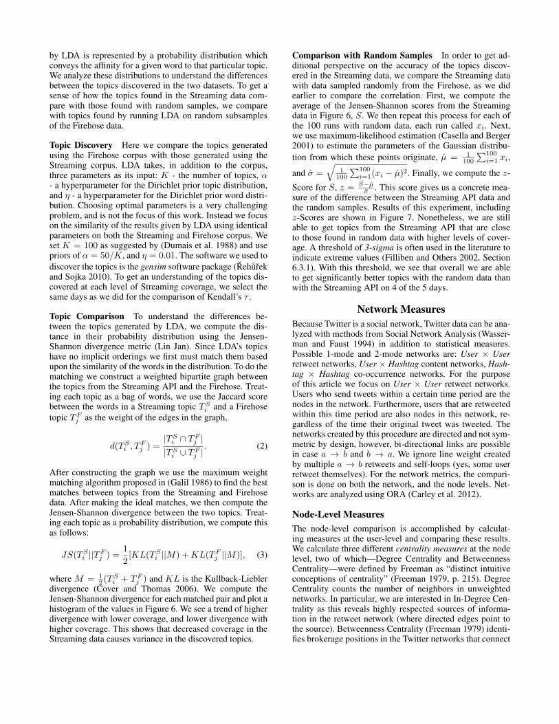
divergence (Cover and Thomas 2006). We compute theJensen-Shannon divergence for each matched pair and plot ahistogram of the values in Figure 6. We see a trend of higherdivergence with lower coverage, and lower divergence withhigher coverage. This shows that decreased coverage in theStreaming data causes variance in the discovered topics.

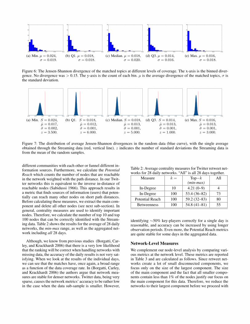
Comparison with Random Samples In order to get ad-ditional perspective on the accuracy of the topics discov-ered in the Streaming data, we compare the Streaming datawith data sampled randomly from the Firehose, as we didearlier to compare the correlation. First, we compute theaverage of the Jensen-Shannon scores from the Streamingdata in Figure 6, S. We then repeat this process for each ofthe 100 runs with random data, each run called xi. Next,we use maximum-likelihood estimation (Casella and Berger2001) to estimate the parameters of the Gaussian distribu-tion from which these points originate, µ = 1

100

∑100i=1 xi,

and σ =√

1100

∑100i=1(xi − µ)2. Finally, we compute the z-

Score for S, z = S−µσ . This score gives us a concrete mea-

sure of the difference between the Streaming API data andthe random samples. Results of this experiment, includingz-Scores are shown in Figure 7. Nonetheless, we are stillable to get topics from the Streaming API that are closeto those found in random data with higher levels of cover-age. A threshold of 3-sigma is often used in the literature toindicate extreme values (Filliben and Others 2002, Section6.3.1). With this threshold, we see that overall we are ableto get significantly better topics with the random data thanwith the Streaming API on 4 of the 5 days.

Network MeasuresBecause Twitter is a social network, Twitter data can be ana-lyzed with methods from Social Network Analysis (Wasser-man and Faust 1994) in addition to statistical measures.Possible 1-mode and 2-mode networks are: User × Userretweet networks, User × Hashtag content networks, Hash-tag × Hashtag co-occurrence networks. For the purposeof this article we focus on User × User retweet networks.Users who send tweets within a certain time period are thenodes in the network. Furthermore, users that are retweetedwithin this time period are also nodes in this network, re-gardless of the time their original tweet was tweeted. Thenetworks created by this procedure are directed and not sym-metric by design, however, bi-directional links are possiblein case a → b and b → a. We ignore line weight createdby multiple a → b retweets and self-loops (yes, some userretweet themselves). For the network metrics, the compari-son is done on both the network, and the node levels. Net-works are analyzed using ORA (Carley et al. 2012).

Node-Level MeasuresThe node-level comparison is accomplished by calculat-ing measures at the user-level and comparing these results.We calculate three different centrality measures at the nodelevel, two of which—Degree Centrality and BetweennessCentrality—were defined by Freeman as “distinct intuitiveconceptions of centrality” (Freeman 1979, p. 215). DegreeCentrality counts the number of neighbors in unweightednetworks. In particular, we are interested in In-Degree Cen-trality as this reveals highly respected sources of informa-tion in the retweet network (where directed edges point tothe source). Betweenness Centrality (Freeman 1979) identi-fies brokerage positions in the Twitter networks that connect

0.00 0.05 0.10 0.15 0.200

10

20

30

40

50

(a) Min. µ = 0.024,σ = 0.019.

0.00 0.05 0.10 0.15 0.200

10

20

30

40

50

(b) Q1. µ = 0.018,σ = 0.018.

0.00 0.05 0.10 0.15 0.200

10

20

30

40

50

(c) Median. µ = 0.018,σ = 0.020.

0.00 0.05 0.10 0.15 0.200

10

20

30

40

50

(d) Q3. µ = 0.014,σ = 0.016.

0.00 0.05 0.10 0.15 0.200

10

20

30

40

50

(e) Max. µ = 0.016,σ = 0.018.

Figure 6: The Jensen-Shannon divergence of the matched topics at different levels of coverage. The x-axis is the binned diver-gence. No divergence was > 0.15. The y-axis is the count of each bin. µ is the average divergence of the matched topics, σ isthe standard deviation.

0.00 0.01 0.02 0.03 0.04 0.05

(a) Min. S = 0.024,µ = 0.017,σ = 0.002,z = 3.500.

0.00 0.01 0.02 0.03 0.04 0.05

(b) Q1. S = 0.018,µ = 0.012,σ = 0.001,z = 6.000.

0.00 0.01 0.02 0.03 0.04 0.05

(c) Median. S = 0.018,µ = 0.013,σ = 0.001,z = 5.000.

0.00 0.01 0.02 0.03 0.04 0.05

(d) Q3. S = 0.014,µ = 0.013,σ = 0.001,z = 1.000.

0.00 0.01 0.02 0.03 0.04 0.05

(e) Max. S = 0.016,µ = 0.013,σ = 0.001,z = 3.000.

Figure 7: The distribution of average Jensen-Shannon divergences in the random data (blue curve), with the single averageobtained through the Streaming data (red, vertical line). z indicates the number of standard deviations the Streaming data isfrom the mean of the random samples.

different communities with each other or funnel different in-formation sources. Furthermore, we calculate the PotentialReach which counts the number of nodes that are reachablein the network weighted with the path distance. In our Twit-ter networks this is equivalent to the inverse in-distance ofreachable nodes (Sabidussi 1966). This approach results ina metric that finds sources of information (users) that poten-tially can reach many other nodes on short path distances.Before calculating these measures, we extract the main com-ponent and delete all other nodes (see next sub-section). Ingeneral, centrality measures are used to identify importantnodes. Therefore, we calculate the number of top 10 and top100 nodes that can be correctly identified with the Stream-ing data. Table 2 shows the results for the average of 28 dailynetworks, the min-max range, as well as the aggregated net-work including all 28 days.

Although, we know from previous studies (Borgatti, Car-ley, and Krackhardt 2006) that there is a very low likelihoodthat the ranking will be correct when handling networks withmissing data, the accuracy of the daily results is not very sat-isfying. When we look at the results of the individual days,we can see that the matches have, once again, a broad rangeas a function of the data coverage rate. In (Borgatti, Carley,and Krackhardt 2006) the authors argue that network mea-sures are stable for denser networks. Twitter data, being verysparse, causes the network metrics’ accuracy to be rather lowin the case when the data sub-sample is smaller. However,

Table 2: Average centrality measures for Twitter retweet net-works for 28 daily networks. “All” is all 28 days together.

Measure k = Top−k(min-max)

All

In-Degree 10 4.21 (0–9) 4In-Degree 100 53.4 (36–82) 73

Potential Reach 100 59.2 (32–83) 80Betweenness 100 54.8 (41–81) 55

identifying ∼50% key-players correctly for a single day isreasonable, and accuracy can be increased by using longerobservation periods. Even more, the Potential Reach metricsare quite stable for some days in the aggregated data.

Network-Level MeasuresWe complement our node-level analysis by comparing vari-ous metrics at the network level. These metrics are reportedin Table 3 and are calculated as follows. Since retweet net-works create a lot of small disconnected components, wefocus only on the size of the largest component. The sizeof the main component and the fact that all smaller compo-nents contain less than 1% of the nodes justify our focus onthe main component for this data. Therefore, we reduce thenetworks to their largest component before we proceed with

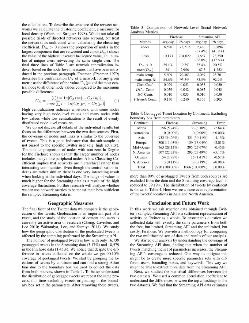
the calculations. To describe the structure of the retweet net-works we calculate the clustering coefficient, a measure forlocal density (Watts and Strogatz 1998). We do not take allpossible triads of directed networks into account, but treatthe networks as undirected when calculating the clusteringcoefficient. Din > 0 shows the proportion of nodes in thelargest component that are retweeted and max(Din) showsthe value of the highest unscaled In-Degree value, i.e., num-ber of unique users retweeting the same single user. Thefinal three lines of Table 3 are network centralization in-dexes based on the node-level measures that have been intro-duced in the previous paragraph. Freeman (Freeman 1979)describes the centralization CX of a network for any givenmetric as the difference of the valueCX(p∗) of the most cen-tral node to all other node values compared to the maximumpossible difference:

CX =

∑i = 1n[CX(p∗)− CX(pi)]

max∑i = 1n[CX(p∗)− CX(pi)]

(4)

High centralization indicates a network with some nodeshaving very high node-level values and many nodes withlow values while low centralization is the result of evenlydistributed node-level measures.

We do not discuss all details of the individual results butfocus on the differences between the two data sources. First,the coverage of nodes and links is similar to the coverageof tweets. This is a good indicator that the sub-sample isnot biased to the specific Twitter user (e.g. high activity).The smaller proportion of nodes with non-zero In-Degreefor the Firehose shows us that the larger number of nodesincludes many more peripheral nodes. A low Clustering Co-efficient implies that networks are hierarchical rather thaninteracting communities. Even though the centralization in-dexes are rather similar, there is one very interesting resultwhen looking at the individual days: The range of values ismuch higher for the Streaming data as a result of the highcoverage fluctuation. Further research will analyze whetherwe can use network metrics to better estimate how sufficientthe sampled Streaming data is.

Geographic MeasuresThe final facet of the Twitter data we compare is the geolo-cation of the tweets. Geolocation is an important part of atweet, and the study of the location of content and users iscurrently an active area of research (Cheng, Caverlee, andLee 2010; Wakamiya, Lee, and Sumiya 2011). We studyhow the geographic distribution of the geolocated tweets isaffected by the sampling performed by the Streaming API.

The number of geotagged tweets is low, with only 16,739geotagged tweets in the Streaming data (3.17%) and 18,579in the Firehose data (1.45%). We notice that despite the dif-ference in tweets collected on the whole we get 90.10%coverage of geotagged tweets. We start by grouping the lo-cations of tweets by continent and can find a strong Asianbias due to the boundary box we used to collect the datafrom both sources, shown in Table 1. To better understandthe distribution of geotagged tweets we repeat the same pro-cess, this time excluding tweets originating in the bound-ary box set in the parameters. After removing these tweets,

Table 3: Comparison of Network-Level Social NetworkAnalysis Metrics.

Firehose Streaming APIMetrics avg.day 28 days avg.day 28 daysnodes 6,590 73,719 2,466

(37.4%)30,894(41.9%)

links 10,173 204,022 3,667(36.0%)

76,750(37.6%)

Din > 0 25.1% 19.3% 32.4% 20.5%max(Din) 341 2,956 167.3 1,252main comp. 5,609 70,383 2,069 28,701

main comp. % 84.6% 95.5% 82.5% 92.9%Clust.Coef. 0.029 0.053 0.033 0.050DCin Centr. 0.059 0.042 0.085 0.043BC Centr. 0.010 0.053 0.010 0.050

PReach Centr. 0.130 0.240 0.156 0.205

Table 4: Geotagged Tweet Location by Continent. Excludingboundary box from parameters.

Continent Firehose Streaming ErrorAfrica 156 (5.74%) 33 (3.10%) -2.64%

Antarctica 0 (0.00%) 0 (0.00%) ±0.00%Asia 932 (34.26%) 321 (30.11%) -4.15%

Europe 300 (11.03%) 139 (13.04%) +2.01%Mid-Ocean 765 (28.12%) 295 (27.67%) -0.45%N. America 607 (22.32%) 293 (27.49%) +5.17%

Oceania 54 (1.98%) 15 (1.41%) -0.57%S. America 3 (0.11%) 2 (0.19%) +0.08%

Total 2720 (100.00%) 1066 (100.00%) ±0.00%

more than 90% of geotagged Tweets from both sources areexcluded from the data and the Streaming coverage level isreduced to 39.19%. The distribution of tweets by continentis shown in Table 4. Here we see a more even representationof the tweets’ locations in Asia and North America.

Conclusion and Future WorkIn this work we ask whether data obtained through Twit-ter’s sampled Streaming API is a sufficient representation ofactivity on Twitter as a whole. To answer this question wecollected data with exactly the same parameters from boththe free, but limited, Streaming API and the unlimited, butcostly, Firehose. We provide a methodology for comparingthe two multifaceted sets of data and results of our analysis.

We started our analysis by understanding the coverage ofthe Streaming API data, finding that when the number oftweets matching the set of parameters increases, the Stream-ing API’s coverage is reduced. One way to mitigate thismight be to create more specific parameter sets with dif-ferent users, bounding boxes, and keywords. This way wemight be able to extract more data from the Streaming API.

Next, we studied the statistical differences between thetwo datasets. We used a common correlation coefficient tounderstand the differences between the top n hashtags in thetwo datasets. We find that the Streaming API data estimates

the top hashtags for a large n well, but is often misleadingwhen n is small. We also employed LDA to extract topicsfrom the text. We compare the probability distribution of thewords from the most closely-matched topics and find thatthey are most similar when the coverage of the StreamingAPI is greatest. That is, topical analysis is most accuratewhen we get more data from the Streaming API.

The Streaming API provides just one example of howsampling Twitter data affects measures. We leverage theFirehose data to get additional samples to better understandthe results from the Streaming API. In both of the above ex-periments we compare the Streaming data with 100 datasetssampled randomly from the Firehose data. We compare thestatistical properties to find that the Streaming API performsworse than randomly sampled data, especially at low cov-erage. We find that in the case of top hashtag analysis, theStreaming API sometimes reveals negative correlation in thetop hashtags, while the randomly sampled data exhibits veryhigh positive correlation with the Firehose data. In the caseof LDA we find a significant increase in the accuracy ofLDA with the randomly sampled data over the data fromthe Streaming API. Both of these results indicate some biasin the way that the Streaming API provides data to the user.

By analyzing retweet User×User networks we were ableto show that we can identify, on average, 50–60% of the top100 key-players when creating the networks based on oneday of Streaming API data. Aggregating some days of datacan increase the accuracy substantially. For network levelmeasures, first in-depth analysis revealed interesting corre-lation between network centralization indexes and the pro-portion of data covered by the Streaming API.

Finally, we inspect the properties of the geotagged tweetsfrom both sources. Surprisingly, we find that the StreamingAPI almost returns the complete set of the geotagged tweetsdespite sampling. We attribute this to the geographic bound-ary box. Although the number of geotagged tweets is stillvery small in general (∼1%), researchers using this informa-tion can be confident that they work with an almost completesample of Twitter data when geographic boundary boxes areused for data collection. When we remove the tweets col-lected this way, we see a much larger disparity in the tweetsfrom both datasets. Even with this disparity, we see a similardistribution based on continent.

Overall, we find that the results of using the StreamingAPI depend strongly on the coverage and the type of anal-ysis that the researcher wishes to perform. This leads to thenext question concerning the estimation of how much datawe actually get in a certain time period. We suggest that wefound first evidence in different types of analysis that canhelp us to estimate the Streaming API coverage. Uncoveringthe nuances of the Streaming API will help researchers, busi-ness analysts, and governmental institutions to better groundtheir scientific results based on Twitter data.

Looking forward, we hope to find methods to compensatefor the biases in the Streaming API to provide a more accu-rate picture of Twitter activity to researchers. Provided fur-ther access to Twitter’s Firehose, we will determine whetherthe methodology presented here will yield similar results forTwitter data collected from other domains, such as natural

disaster, protest, and elections.

AcknowledgementsThis work is sponsored in part by Office of Naval Researchgrants N000141010091 and N000141110527. We thank LeiTang for thoughtful advice and discussion throughout thedevelopment of this work.

ReferencesAgresti, A. 2010. Analysis of Ordinal Categorical Data,volume 656. Hoboken, New Jersey: Wiley.Blei, D. M.; Ng, A. Y.; and Jordan, M. I. 2003. Latent dirich-let allocation. The Journal of Machine Learning Research3:993–1022.Borgatti, S. P.; Carley, K. M.; and Krackhardt, D. 2006.On the robustness of centrality measures under conditionsof imperfect data. Social Networks 28(2):124–136.Campbell, D. G. 2011. Egypt Unshackled: Using SocialMedia to @#:) the System. Amherst, NY: Cambria Books.Carley, K. M.; Pfeffer, J.; Reminga, J.; Storrick, J.; andColumbus, D. 2012. ORA User’s Guide 2012. Technical Re-port CMU-ISR-12-105, Carnegie Mellon University, Schoolof Computer Science, Institute for Software Research, Pitts-burgh, PA.Casella, G., and Berger, R. L. 2001. Statistical Inference.Belmont, CA: Duxbury Press.Chae, J.; Thom, D.; Bosch, H.; Jang, Y.; Maciejewski, R.;Ebert, D. S.; and Ertl, T. 2012. Spatiotemporal Social MediaAnalytics for Abnormal Event Detection and Examinationusing Seasonal-Trend Decomposition. In Proceedings of theIEEE Conference on Visual Analytics Science and Technol-ogy. Brighton, UK: IEEE Conference on Visual AnalyticsScience and Technology.Cheng, Z.; Caverlee, J.; and Lee, K. 2010. You Are WhereYou Tweet: A Content-Based Approach to Geo-locatingTwitter Users. In Proceedings of The 19th ACM Inter-national Conference on Information and Knowledge Man-agement, 759–768. Toronto, Ontario, Canada: InternationalConference on Information and Knowledge Management.Costenbader, E., and Valente, T. W. 2003. The stabilityof centrality measures when networks are sampled. Socialnetworks 25(4):283–307.Cover, T. M., and Thomas, J. A. 2006. Elements of Infor-mation Theory. Hoboken, New Jersey: Wiley InterScience.De Choudhury, M.; Lin, Y.-R.; Sundaram, H.; Candan, K. S.;Xie, L.; and Kelliher, A. 2010. How Does the Data SamplingStrategy Impact the Discovery of Information Diffusion inSocial Media. In Proc. of the 4th Int’l AAAI Conference onWeblogs and Social Media, 34–41. Washington, DC, USA:AAAI.De Longueville, B.; Smith, R. S.; and Luraschi, G. 2009.”omg, from here, i can see the flames!”: a use case of mininglocation based social networks to acquire spatio-temporaldata on forest fires. In Proceedings of the 2009 Interna-tional Workshop on Location Based Social Networks, LBSN’09, 73–80. New York, NY, USA: ACM.

Dumais, S. T.; Furnas, G. W.; Landauer, T. K.; Deerwester,S.; and Harshman, R. 1988. Using latent semantic analysisto improve access to textual information. In Proceedingsof the SIGCHI Conference on Human Factors in ComputingSystems, CHI ’88, 281–285. New York, NY, USA: ACM.Efron, M. 2010. Hashtag retrieval in a microblogging en-vironment. In Proc. of the 33rd international ACM SIGIRconference on Research and development in information re-trieval, SIGIR ’10, 787–788. New York, NY, USA: ACM.Filliben, J. J., and Others. 2002. NIST/SEMTECHEngineering Statistics Handbook. Gaithersburg:www.itl.nist.gov/div898/handbook, NIST.Freeman, L. C. 1979. Centrality in Social Networks: Con-ceptual clarification. Social Networks 1(3):215–239.Galil, Z. 1986. Efficient algorithms for finding maximummatching in graphs. ACM Comput. Surv. 18(1):23–38.Gayo-Avello, D.; Metaxas, P. T.; and Mustafaraj, E. 2011.Limits of electoral predictions using twitter. In Proceedingsof the International Conference on Weblogs and Social Me-dia, volume 21, 490–493. Barcelona, Spain: AAAI.Granovetter, M. 1976. Network Sampling: Some First Steps.American Journal of Sociology 81(6):1287–1303.Hong, L., and Davison, B. D. 2010. Empirical study of topicmodeling in twitter. In Proc. First Workshop on Social Me-dia Analytics, SOMA ’10, 80–88. NYC, NY, USA: ACM.Hong, L.; Ahmed, A.; Gurumurthy, S.; Smola, A. J.; andTsioutsiouliklis, K. 2012. Discovering geographical topicsin the twitter stream. In Proceedings of the 21st interna-tional conference on World Wide Web, WWW ’12, 769–778.New York, NY, USA: ACM.Joseph, K.; Tan, C. H.; and Carley, K. M. 2012. Beyond “lo-cal”, “categories” and “friends”: clustering foursquare userswith latent “topics”. In Proceedings of the 2012 ACM Con-ference on Ubiquitous Computing, UbiComp ’12, 919–926.New York, NY, USA: ACM.Kireyev, K.; Palen, L.; and Anderson, K. 2009. Applicationsof Topics Models to Analysis of Disaster-Related TwitterData. In NIPS Workshop on Applications for Topic Models:Text and Beyond, volume 1.Kossinets, G. 2006. Effects of missing data in social net-works. Social Networks 28(3):247–268.Kumar, S.; Barbier, G.; Abbasi, M. A.; and Liu, H. 2011.Tweettracker: An analysis tool for humanitarian and disasterrelief. In Fifth International AAAI Conference on Weblogsand Social Media. Barcelona Spain: AAAI.Leskovec, J., and Faloutsos, C. 2006. Sampling from LargeGraphs. In Proceedings of the 12th ACM SIGKDD Interna-tional Conference on Knowledge Discovery and Data Min-ing, 631–636.Lin, J. Jan. Divergence measures based on the shan-non entropy. Information Theory, IEEE Transactions on37(1):145–151.Mathioudakis, M., and Koudas, N. 2010. Twittermonitor:trend detection over the twitter stream. In Proc. of the 2010ACM SIGMOD Int’l Conference on Management of data,SIGMOD ’10, 1155–1158. New York, NY, USA: ACM.

Pozdnoukhov, A., and Kaiser, C. 2011. Space-time dynam-ics of topics in streaming text. In Proc. of the 3rd ACMSIGSPATIAL Int’l Workshop on Location-Based Social Net-works, LBSN ’11, 1–8. New York, NY, USA: ACM.Recuero, R., and Araujo, R. 2012. On the rise of artificialtrending topics in twitter. In Proceedings of the 23rd ACMconference on Hypertext and social media, HT ’12, 305–306. New York, NY, USA: ACM.Rehurek, R., and Sojka, P. 2010. Software Framework forTopic Modelling with Large Corpora. In Proc. of the LREC2010 Workshop on New Challenges for NLP Frameworks,45–50. Valletta, Malta: ELRA.Sabidussi, G. 1966. The centrality index of a graph. Psy-chometrika 69:581–603.Sofean, M., and Smith, M. 2012. A real-time architecture fordetection of diseases using social networks: design, imple-mentation and evaluation. In Proceedings of the 23rd ACMconference on Hypertext and social media, HT ’12, 309–310. New York, NY, USA: ACM.Tsur, O., and Rappoport, A. 2012. What’s in a hashtag?:content based prediction of the spread of ideas in microblog-ging communities. In Proceedings of the fifth ACM interna-tional conference on Web search and data mining, WSDM’12, 643–652. New York, NY, USA: ACM.Tumasjan, A.; Sprenger, T. O.; Sandner, P. G.; and Welpe,I. M. 2010. Predicting elections with twitter: What 140characters reveal about political sentiment. In Proceedingsof the International Conference on Weblogs and Social Me-dia, 178–185. Washington, DC, USA: AAAI.Wakamiya, S.; Lee, R.; and Sumiya, K. 2011. Crowd-basedurban characterization: extracting crowd behavioral patternsin urban areas from twitter. In Proc. of the 3rd ACM SIGSPA-TIAL Int’l Workshop on Location-Based Social Networks,LBSN ’11, 77–84. New York, NY, USA: ACM.Wasserman, S., and Faust, K. 1994. Social Network Analy-sis: Methods and Applications. Cambridge, MA: CambridgeUniversity Press.Watts, D. J., and Strogatz, S. H. 1998. Collective dynamicsof ’small-world’ networks. Nature 393:440–442.Yang, L.; Sun, T.; Zhang, M.; and Mei, Q. 2012. We knowwhat @you #tag: does the dual role affect hashtag adoption?In Proc. of the 21st int’l conference on World Wide Web,WWW ’12, 261–270. New York, NY, USA: ACM.Yin, Z.; Cao, L.; Han, J.; Zhai, C.; and Huang, T. 2011.Geographical topic discovery and comparison. In Proceed-ings of the 20th international conference on World wide web,WWW ’11, 247–256. New York, NY, USA: ACM.