Embed Size (px)
Citation preview

IS PRICING ABOVE MARGINAL COST AN INDICATION OF
MARKET POWER IN THE U.S. MEATPACKING INDUSTRY?
Dimitrios Panagiotou Graduate Student
Department of Agricultural Economics University of Nebraska-Lincoln
308E H.C. Filley Hall Lincoln, NE 68583-0922 Phone: (402) 472-9143
Selected paper prepared for presentation at the American Agricultural Economics Association
Annual Meeting, Providence, Rhode Island, 24-27 July 2005
Copyright 2005 by Dimitrios Panagiotou. All rights reserved. Readers may make verbatim copies of this document for non-commercial purposes by any means, provided that this copyright notice appears on all such copies.

2
IS PRICING ABOVE MARGINAL COST AN INDICATION OF
MARKET POWER IN THE U.S. MEATPACKING INDUSTRY? Abstract: There have been concerns about the increasing concentration in
the meat packing industry. But this increased concentration may be due to
various types of cost economies. In this paper we prove the existence of
scale economies that might justify the increased consolidation in the
industry.
.

3
IS PRICING ABOVE MARGINAL COST AN INDICATION OF
MARKET POWER IN THE U.S. MEATPACKING INDUSTRY?
1.1 Statement of the Problem
Many times we have heard the expression “extraction of market
power” or “oligopolistic conditions” for a specific industry. This means that
firms in that market price above marginal cost of production. Figure 1 below
shows what is happening in the specific industry.
P
Q
D
MR
MC
P1
Q1
MC1
AC
Figure 1
But is it really pricing above marginal cost an indication of exercising
market power or is it the result of cost economies under which firms operate

4
in this industry? In this case Figure 2 represents what is happening for a
representative firm in the industry.
AC
MC
Q
P
MC
Q1
P1
MR
D1
Figure 2
As we can see from figure 2, the price in this industry is above marginal
cost, but there is no exertion of market power. The industry in order to
avoid losses, prices its product above marginal cost where price equals
average cost and consequently economic profits equal zero.
Thus, before we make rush judgments about the degree of
competitiveness of an industry as concentration increases, we should take into
account any cost economies that might exist. By cost economies we mean

5
short-run (utilization), long-run (scale), scope (output jointness) and multi-plant
(information and risk-sharing) may provide incentives for expanding output,
size, diversification, and plant numbers.
In this paper we are going to find out what is really happening in the
U.S. meatpacking industry. Is it really the case that firms exercise market
power in this market, or the situation described in figure 2 characterizes the
specific industry?
1.2 Literature Review
Paul Cathy Morrison in her paper: “Market and Cost Structure in the
U.S. Beef Packing Industry: A Plant Level Analysis.” American Journal of
Agricultural Economics 83(1) (February 2001), pp.64-76, comments that
increasing size of plants and firms in the beef-packing industry could also be
indicative of the efficiency potential from scale, scope, multi-plant, and
other types of cost economies, which could allow larger and more diverse or
specialized plants or firms to increase their cost effectiveness. Modeling and
measuring the market power and technological structure in this industry to
explore these questions involves appropriate representation of both the
oligopsony/poly nature of the industry, and the production/cost structure.
Characterization of market power depends on the cost structure, because it

6
involves comparing the average prices of an output or input to its associated
marginal valuation – the marginal shadow value for the input, or the
marginal cost for the output. Careful representation of costs, with
recognition of scale, size, utilization, and scope economies, is therefore
important to the construction of the market power. Her results indicated
little if any existence of market power in the beef-packing industry, and
significant cost economies in this industry.
Paul Cathy Morrison in her paper: “Cost Economies and Market
power: The case of the U.S. Meat Packing Industry.” The review of
Economics and statistics 83(3) (August 2001), pp.531-540, by utilizing a
dynamic model based on a restricted Generalized -Leontief cost function
finds out significant but declining market power and cost economies in the
U.S. meat packing industry. Analysis of the cost structure, suggests
utilization issues and long-run scale economies being the main forces
driving expansion in the scale of production.
This paper differs from the above mentioned papers in the sense that
we have no input fixities. We test our model within a long-run framework,
where everything is flexible.
Finally this paper is related to the master’s thesis of D. Panagiotou:
“Cointegration, Error Correction and the Measurement of Oligopsony
7
Conduct in the U.S. Cattle Market”, 2002, University of Nebraska-Lincoln,
because it moves downstream in the marketing channel. That paper used an
error correction model to find out if beef packers (which can be considered a
category of meatpackers) exert oligopsony power when they purchase their
primary input: cattle. The assumption there was that the packers are price
takers when they sell their product. The results indicated no market power in
the short-run as well as in the long-run. In this paper we assume that
packers are price takers when they purchase cattle, but they might exert
market power when they sell their output.
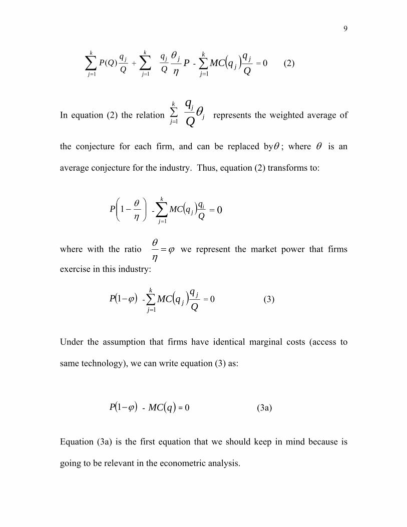
2. Theoretical framework
We make use of the framework that E. Appelbaum uses in his paper:
“The Estimation of the Degree of Oligopoly Power.” (Journal of
Econometrics 9(1979), pp.287-299). We consider a possible non-
competitive industry, in which j firms produce a homogeneous (in the eyes
of the consumer) output Q (meat), with each firm producing qj. Each firm
uses m inputs X1,…..Xm, in order to produce the desirable output.
Let the inverse market demand curve facing the industry be given by
P = P(Q). Then the Profit function for each firm can be written as:
Пj= P(Q) qj - ( )jqC

8
From the first order conditions we get:
j
j
q∂Π∂
= P(Q) + jq jq
QQP∂∂
∂∂
- ( )qjqC j
∂
∂= 0
P(Q) + jq PP
QP
j∂∂
∂∂
- MC( jq ) = 0 (1)
In equation (1), the second term of the summation includes the inverse of the
demand elasticity of the industry,
η1
=∂∂
PQ
QP
and the conjecture for each firm:
j
j qQ
∂∂
=θ
Thus, equation (1) can be written:
P(Q) + P (Q) ηθ j
- MC( jq ) = 0
If we aggregate across the firms of the industry, and at the same time
multiply each term by Qq j we are going to get:
9
QP jk
j∑=1
)( + Qqj
k
j∑=1
Pj
ηθ
qMC jk
jj∑
=1 = 0 (2)
In equation (2) the relation jjk
j Qqθ∑
=1represents the weighted average of
the conjecture for each firm, and can be replaced byθ ; where θ is an
average conjecture for the industry. Thus, equation (2) transforms to:
⎟⎟⎠
⎞⎜⎜⎝
⎛−ηθ1P - ( )
QqqMC i
k
jj∑
=1 = 0
where with the ratio ϕηθ= we represent the market power that firms
exercise in this industry:
( )ϕ−1P - ( )Qq
qMC jk
jj∑
=1 = 0 (3)
Under the assumption that firms have identical marginal costs (access to
same technology), we can write equation (3) as:
( )ϕ−1P - ( )qMC = 0 (3a)
Equation (3a) is the first equation that we should keep in mind because is
going to be relevant in the econometric analysis.

10
Now we are going to look at the cost structure of the industry, in order to use
it for the derivation and estimation of the marginal cost, the average cost.
We are doing this because it is going to be very helpful in our analysis for
the cost economies that might exist in this industry.
If we let the cost function to be represented by a Generalized-Leontief
function, then the total cost for each firm can be written as:
( ) ( ) ( ) ( ) njiwbqgwwdqhqC i
n
iijmi
n
i
n
mimjj ,...1,;
11 1
5.0 =∀+= ∑∑ ∑== =
and the marginal cost can be derived as:
( ) ( ) ( ) ( ) njiwbqgwwdqhqqC
i
n
iijqmi
n
i
n
mimjq
j
j ,...1,;1
5.0
1 1=∀+=
∂∂
∑∑ ∑== =
In this paper we are going to use the following specifications:
( ) jj qqh = and ( ) 2jj qqg = .
These are specifications that Olson and Shien (1989) and Baffles and
Vasavada (1989) first introduced (see references for their papers):
Thus, the marginal cost takes the form:
( ) ( ) i
n
iimi
n
i
n
mim
j
j wbqwwdqqC
∑∑∑== =
+=∂∂
1
5.0
1 12 (4)

11
If we additionally assume that the firms use m inputs, then for the
Generalized- Leontief cost function, the optimal input demand functions are
going to be given by:
( )=
∂
∂≡
i
ji w
qCX ( ) ijim
n
mimj bqwwdq 25.0
1/ +∑
=
and dividing by qj we get:
≡ji qX / ( ) ijim
n
mim bqwwd +∑
=
5.0
1/ mi ,....1=∀ (5)
Combining equations (3) and (5) we are going to get a system of equations,
with the help of which we can estimate the parameters of the cost function as
well as the index of market powerϕ .
From our function specification for the cost we use in this paper we
already derived the marginal cost in equation (4). The average cost for the
Generalized- Leontief cost function we use in this paper is:
AC = =qC
( ) i
n
iimi
n
i
n
mim wbqwwd ∑∑ ∑
== =+
1
5.0
1 1 (6)
Dividing equation (4) with equation (6) we get:
=ACMC
( ) /]2[1
5.0
1 1i
n
iimi
n
i
n
mim wbqwwd ∑∑ ∑
== =+ [ ( ) i
n
iimi
n
i
n
mim wbqwwd ∑∑ ∑
== =+
1
5.0
1 1] (7)

12
As we can observe in equation (7), if i
n
ii wb∑
=1 is negative, then MC is
less than AC and we have cost economies, which in our case is going to be
scale economies (size increase), since we examine the industry in a long-run
framework. So in this case figure 2 is going to give us the best picture about
what is happening in the industry.
If i
n
ii wb∑
=1 is positive, then MC is greater than AC then there is no
indication about cost economies, and figure 1 is relevant in our analysis for
this case.
If i
n
ii wb∑
=1 is not statistically different than zero, then MC is equal to
AC and we have constant returns to scale, and firms are making zero
economic profits.
If φ = 0 then price equals marginal cost from equation (3a), and in the
long-run we are going to have an equilibrium where price equals marginal
cost and both of them equal the long average cost, and that’s the case where
we have zero economic profits and exertion of market power in the specific
industry.

13
3. Econometric application
3.1 Data
We use data from 1958 to 1996 for the U.S meatpacking industry,
obtained from the National Bureau of Economic Research. The data include
observations on the slaughtering of cattle, hogs, sheep, lambs, and calves for
meat to be sold or to be used in canning, cooking, curing, and freezing, and
in making sausage, lard, and other products.
We have four competitively priced inputs, labor (XL), capital (XK),
materials (XM), and energy (XE) whose prices are WL, WK, WM, WE
respectively and Q is the quantity produced and piship is the price of the
product. In the appendix there is a description of the data:
3.2 Empirical results
The Generalized-Leontief cost function in equation (4) takes the form:
( ) ( ) ii
imii m
im wbqwwdqqC ∑∑ ∑== =
+=4
1
25.04
1
4
1,
and we are going to have four equations, one for each input, of the form:
≡qX i / ( ) iimm
im bqwwd +∑=
5.04
1/

14
For empirical implementation the model has to be estimated within a
stochastic framework. To do this, we assume that equations are stochastic
due to errors in optimization.
Although the equation by equation OLS estimation might appear
attractive, since the equations are linear in the parameters, these demand
equations have cross-equation symmetry constraints, and the OLS method is
not going to impose the symmetry condition. In our study we use the
Zellner’s seemingly unrelated estimator (ZEF) in order to obtain efficient
parameter estimates.
We define the additive disturbance term in the ith equation at the time t
as ei(t), t=1,….,T. We also define the column vector of disturbances at the
time t as et. We also assume that the vector of disturbances is jointly
normally distributed with mean vector zero and non-singular covariance
matrix Ω,
( ) ( )[ ] Ω=′Ε tese jj if t = s,
= 0 if t ≠ s.
Estimating the system of the four equations along with equation (3a), we get
the following results:
15
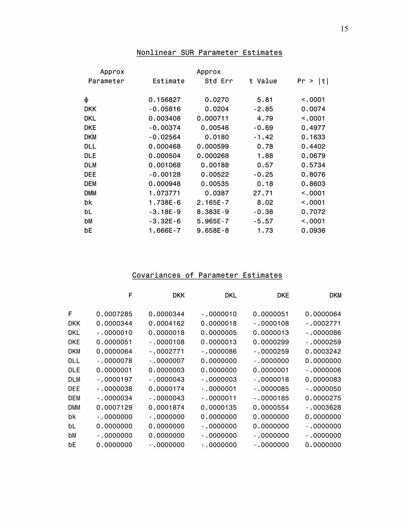
Nonlinear SUR Parameter Estimates Approx Approx Parameter Estimate Std Err t Value Pr > |t| φ 0.156827 0.0270 5.81 <.0001 DKK -0.05816 0.0204 -2.85 0.0074 DKL 0.003408 0.000711 4.79 <.0001 DKE -0.00374 0.00546 -0.69 0.4977 DKM -0.02564 0.0180 -1.42 0.1633 DLL 0.000468 0.000599 0.78 0.4402 DLE 0.000504 0.000268 1.88 0.0679 DLM 0.001068 0.00188 0.57 0.5734 DEE -0.00128 0.00522 -0.25 0.8076 DEM 0.000948 0.00535 0.18 0.8603 DMM 1.073771 0.0387 27.71 <.0001 bk 1.738E-6 2.165E-7 8.02 <.0001 bL -3.18E-9 8.383E-9 -0.38 0.7072 bM -3.32E-6 5.965E-7 -5.57 <.0001 bE 1.666E-7 9.658E-8 1.73 0.0936
Covariances of Parameter Estimates
F DKK DKL DKE DKM F 0.0007285 0.0000344 -.0000010 0.0000051 0.0000064 DKK 0.0000344 0.0004162 0.0000018 -.0000108 -.0002771 DKL -.0000010 0.0000018 0.0000005 0.0000013 -.0000086 DKE 0.0000051 -.0000108 0.0000013 0.0000299 -.0000259 DKM 0.0000064 -.0002771 -.0000086 -.0000259 0.0003242 DLL -.0000078 -.0000007 0.0000000 -.0000000 0.0000000 DLE 0.0000001 0.0000003 0.0000000 0.0000001 -.0000006 DLM -.0000197 -.0000043 -.0000003 -.0000018 0.0000083 DEE -.0000038 0.0000174 -.0000001 -.0000085 -.0000050 DEM -.0000034 -.0000043 -.0000011 -.0000185 0.0000275 DMM 0.0007129 0.0001874 0.0000135 0.0000554 -.0003628 bk -.0000000 -.0000000 0.0000000 0.0000000 0.0000000 bL 0.0000000 0.0000000 -.0000000 0.0000000 -.0000000 bM -.0000000 0.0000000 -.0000000 -.0000000 -.0000000 bE 0.0000000 -.0000000 -.0000000 -.0000000 0.0000000

16
DLL DLE DLM DEE DEM F -7.81E-6 1.4294E-7 -.0000197 -.0000038 -.0000034 DKK -7.325E-7 2.8444E-7 -.0000043 0.0000174 -.0000043 DKL 1.8818E-8 2.9803E-8 -.0000003 -.0000001 -.0000011 DKE -3.859E-8 8.8369E-8 -.0000018 -.0000085 -.0000185 DKM 4.605E-10 -5.525E-7 0.0000083 -.0000050 0.0000275 DLL 3.5909E-7 -1.522E-9 0.0000004 0.0000002 -.0000000 DLE -1.522E-9 7.1594E-8 -.0000001 -.0000002 -.0000010 DLM 3.5419E-7 -1.126E-7 0.0000035 0.0000008 0.0000026 DEE 2.2289E-7 -1.761E-7 0.0000008 0.0000273 -.0000017 DEM -9.37E-9 -9.941E-7 0.0000026 -.0000017 0.0000286 DMM -8.599E-6 3.139E-6 -.0000497 -.0000231 -.0000761 bk 1.575E-11 3.606E-13 -.0000000 -.0000000 0.0000000 bL -4.76E-12 1.439E-13 -.0000000 -.0000000 -.0000000 bM 1.594E-10 -2.34E-11 0.0000000 0.0000000 0.0000000 bE -3.51E-12 1.593E-11 -.0000000 -.0000000 -.0000000 DMM bk bL bM bE F 0.0007129 -9.62E-10 9.845E-11 -1.402E-8 2.413E-11 DKK 0.0001874 -2.841E-9 4.137E-12 2.4087E-9 -7.2E-11 DKL 0.0000135 6.329E-11 -2.06E-13 -4.76E-11 -4.08E-12 DKE 0.0000554 2.917E-11 1.028E-12 -6.45E-11 -6.43E-11 DKM -.0003628 3.522E-10 -7.34E-13 -5.06E-10 1.261E-10 DLL -.0000086 1.575E-11 -4.76E-12 1.594E-10 -3.51E-12 DLE 0.0000031 3.606E-13 1.439E-13 -2.34E-11 1.593E-11 DLM -.0000497 -8.21E-12 -7.92E-12 3.93E-10 -2.22E-11 DEE -.0000231 -6.46E-11 -5.22E-12 5.719E-10 -3.49E-10 DEM -.0000761 4.735E-12 -1.48E-12 1.818E-10 -8.74E-11 DMM 0.0015013 1.2435E-9 1.486E-10 -1.752E-8 6.438E-10 bk 0.0000000 4.689E-14 -7.59E-17 -3.43E-14 5.899E-16 bL 0.0000000 -7.59E-17 7.027E-17 -2.29E-15 1.095E-16 bM -.0000000 -3.43E-14 -2.29E-15 3.558E-13 -1.26E-14 bE 0.0000000 5.899E-16 1.095E-16 -1.26E-14 9.328E-15
As we can observe there is indication of market power, since φ equals
to 0.1568, and is quite significant. But, as we stated in the theoretical
framework we have to check if i
n
ii wb∑
=1 is significantly less than zero:

17
i
n
ii wb∑
=1= kK wb + EEMmLL wbwbwb ++ (8)
where the prices of the factors of production are estimated at the means.
From our estimation of the sum of equation (8) we get:
i
n
ii wb∑
=1= kK wb + EEMmLL wbwbwb ++ = -1.13E-06
and the estimated variance of the sum is found by the multiplication of the
matrices below:
Var ( i
n
ii wb∑
=1) =
= [ ]64.07.05.226577.0
⎥⎥⎥⎥
⎦
⎤
⎢⎢⎢⎢
⎣
⎡
−−−−−−−−−−−−−−−−−−−−−−−−
1533.91426.1161.1169.5143.11356.3153.21443.3
161.1153.21703.7176.7169.51443.3176.7147.4
EEEEEEEE
EEEEEEEE
⎥⎥⎥⎥
⎦
⎤
⎢⎢⎢⎢
⎣
⎡
64.07.05.22
6577.0
= 1.19003E-13
The table below summarizes the results:
Sum -1.13E-06Var 1.19003E-13Se 3.44968E-07t-stat -3.28

18
Thus, as we can see the summation i
n
ii wb∑
=1 is negative, and significantly
different than zero. So, in our case the ratio MC/AC is less than zero, indicating
scale economies in the industry.
4. Conclusion
The purpose of this paper is to examine if in the U.S. meatpacking industry
the indication of pricing above marginal cost is a sign of existence of market
power or Figure 2 describes what is happening in the industry. By utilizing a
Generalized-Leontief cost function, we found out that the estimated parameter
ϕ for the market power is statistically significant, and the ratio of (MC/AC)
is significantly less than one. Hence figure 2 describes what is happening in
the specific industry. Thus, we have low Marginal Cost as compared to
Average Cost, and even though the price mark up is significant, it is supported
by scale economies which are just high enough to allow average costs to be
covered. We use the world scale economies to describe the case of cost
efficiencies (or economies) we have here, because our model examines the
industry within a long-run framework.

19
The above analysis is relevant for antitrust authorities and policies that try
to force downsizing in an industry like the one we analyzed in this paper. The
results indicate that an increase in concentration in the industry might be
welfare enhancing for consumers because it can lead to lower prices because
of the economies of scale. Thus, in this case, increased concentration in an
industry might be socially optimal.

20
Appendix: 1) Description of the Data The SAS System The MEANS Procedure Variable Label N Mean Std Dev Minimum Q Q 39 42580.34 5161.22 29654.34 piship piship 39 0.7305897 0.2986963 0.3350000 wm wm 39 0.6957436 0.2980598 0.3070000 wk wk 39 0.6576923 0.3674194 0.2460000 we we 39 0.6407179 0.4043910 0.2040000 wl wl 39 22.5246080 6.0746394 13.3351186 XK XK 39 356.9177167 72.3127443 243.1208054 XL XL 39 250.4230769 34.5653802 197.6000000 XM XM 39 38879.45 4241.61 29825.36 XE XE 39 284.4098174 40.3584273 224.8826291
Variable Label Maximum Q Q 48917.45 piship piship 1.1990000 wm wm 1.1580000 wk wk 1.2800000 we we 1.1740000 wl wl 29.0935484 XK XK 500.8064516 XL XL 312.7000000 XM XM 46014.80 XE XE 367.4757282
21
References:
Appelbaum, E. “The Estimation of the Degree of Oligopoly Power.” Journal of
Econometrics 9(1979), pp.287-299.
Baffles, J., and U. Vasavada “On the Choice of Functional Forms in Agricultural
Production.” Applied Economics, 21(1989), pp.1053-1061.
Berndt, R.E. “The Practice of Econometrics: Classic and Contemporary.”
Addison- Wesley Publ. Company., 1991.
Bureau of the Census, Longitudinal Research Data Base, Washington, DC:
Bureau of the Census, 1958-96.
Bureau of the Census, Ownership Change Data Base, Washington, DC: Bureau
of the Census, 1958-96.
Capablo, S. and J. Antle. “An Introduction to Recent Development in Production
and Productivity Measurement.” In Agricultural Productivity Measurement
and Explanation, chapter 2. Washington, D.C. : Resources for the Future,
1988.
Chambers, R. “Applied Production Analysis: A Dual Approach.” Cambridge
University Press 1988.
Koutsoyiannis, A. “Modern Microeconomics- Second edition.” The Macmillan
Press LTD 1979.

22
Morrison, C. “Structural Change, Capital Investment and Productivity change in
the Food Processing Industry.” American Journal of Agricultural Economics
79(1997), pp.110-125.
Morrison, C. “Aggregation and the Measurement of Technological and Market
Structure: The Case of the U.S. Meatpacking Industry.” American Journal of
Agricultural Economics 81 (August 2001), pp.624-629.
Morrison, C. “Market and Cost Structure in the U.S. Beef Packing Industry: A
Plant Level Analysis.” American Journal of Agricultural Economics 83(1)
(February 2001), pp.64-76.
Olson, D.O., and Y.N. Shien “Estimating Functional Forms in Cost Prices.”
European Economic Review 33(1989), pp.1445-1461.
Panagiotou, D., “Co-integration, Error Correction, and the Measurement of
Oligopsony Conduct in the U.S. Cattle Market.” Master thesis, UNL, August
2002.
Silberberg, E. and W. Suen. “The Structure of Economics: A Mathematical
Analysis – Third Edition.” Irwin/McGraw-Hill companies 2001.
U.S. Department of Agriculture, Concentration in the Red Meat Packing
Industry, Packers and Stockyards Programs, Grain and inspection, Packers
and Stockyards Administration (May 2005).