1

Is Price Flexibility De-Stabilizing? A Reconsideration

Hamza Ali Malik William M. Scarth Department of Economics Department of Economics Lakehead University McMaster University Thunder Bay, Ontario, P7B 5E1 Hamilton, Ontario, L8S 4M4 hamza.malik@lakeheadu.ca scarth@mcmaster.ca

July 2003

Abstract

Using a new Keynesian model of monetary policy for an open economy, this paper

explores the impact of an increased degree of price flexibility on output volatility.

Previous analysis of this question offered mixed conclusions especially in an open

economy context. We find support for Keynes’ concern that under a flexible exchange

rate regime a lower degree of price flexibility help lower output volatility. This result is

consistent with the behaviour of central banks that argue that their low inflation-flexible

exchange rate policy has decreased the degree of nominal price flexibility. We also find

support for central banks that favour fixed exchange rates. Fixed exchange rate regime

implicitly implies that the economy is willing to accept structural reforms of the sort that

promote flexibility in prices (and wages) to absorb the effects of shocks. In the paper we

find that with fixed exchange rates output volatility indeed goes down as a result of

increased price flexibility. Thus, we find internal consistency within both views about

exchange rate policy.

JEL Classification: E52, F41

Keywords: price flexibility, exchange rate policy, monetary policy in an open economy.

2

1)- Introduction

At least since Keynes (1936), macroeconomists have recognized that a one -time

reduction in the price level involves higher aggregate demand, while an ongoing expected

rate of deflation involves lower aggregate demand. Stressing the second of these two

propositions, Keynes argued that an increased degree of price flexibility leads to

increased output volatility. Perhaps one of the reasons that he favoured the Bretton

Woods arrangements was that he expected (1936, p. 276) the destabilizing feature of

increased price flexibility to be more powerful under flexible exchange rates.

Formal evaluation of Keynes’ concern did not take place until 50 years after he wrote on

the subject. Howitt (1986), Chadha (1988) and Fleming (1987) offered analytical

explorations of this issue, based on the first generation of rational expectations models

(that involved descriptive structural equations). DeLong and Summers (1986), Driskill

and Sheffrin (1986), King (1988) and Myers and Scarth (1990) used numerical versions

of similar models to evaluate Keynes’ concern. Mixed conclusions emerged. For

example, using a closed-economy analysis, DeLong and Summers (1986, p. 1031)

concluded that “simulations based on realistic parameter values suggest that increases in

price flexibility might well increase the cyclical variability of output in the United

States.” In contrast, in a small open-economy setting, Myers and Scarth reported only

very limited support for the proposition that an increased degree of price flexibility leads

to increased output volatility. Further, they found more support for Keynes’ concern if

the exchange rate is fixed – a result that is opposite to what Keynes expected.

3

Since this spate of interest in evaluating the output volatility effects of changes in the

degree of price flexibility, there has been a fundamental change in the focus of policy-

oriented macro theory. The “new neoclassical synthesis” has emerged as the standard

framework, because this compact structure combines three very desirable features. First,

it is firmly grounded in inter-temporal optimization, so the desire on the part of new

classicals for well-articulated micro-foundations is respected. With each equation being

structural, the Lucas critique can be respected as the model is applied to policy questions.

Second, a degree of nominal rigidity is allowed for, so the mechanism that Keynesians

regard as essential for generating short-run real effects from demand shocks is an integral

part of the structure. Third, the model is conveniently analyzed at the same level of

aggregation as was common with earlier generations of policy-oriented discussions. The

purpose of this note is to re-examine the question of de-stabilizing price flexibility in the

context of this new neoclassical framework.

We find it surprising that this reconsideration has yet to be explored. For one thing, this

question is a central one, and with a change in the core framework of mainstream

macroeconomics, one would expect a sensitivity check on all previously derived aspects

of conventional wisdom. But the lack of this checking is particularly surprising given

that, recently, policy makers have taken positions on this very question. For example,

central bankers have noted that average contract length has varied rather dramatically

over the last 30 years – falling as the core inflation rate rose, and rising again as the

underlying inflation rate came back close to zero. It appears to be presumed that longer

contract length (a lower degree of price flexibility) is one of benefits of low equilibrium

4

inflation. That is, it appears that central bankers agree with Keynes on this question. On

the other hand, when answering the concern that their adoption of a common currency

may involve a loss on macroeconomic built -in stability grounds, policy makers in Europe

argue that this very fact may induce agents to embrace structural reforms in a more

thorough-going fashion. One dimension of more flexible labour markets may be an

increased degree of wage flexibility. If so, these analysts appear to be arguing that such

increased flexibility, if it were to develop, would help stabilize real output. In other

words, they disagree with Keynes on this question. It seems that a reconsideration of this

question – within the now-accepted framework for policy analysis – is of relevance for

both these debates.

The remainder of the note is organized as follows. In the next section, a small open

economy version of the new neoclassical synthesis model is outlined. We assume that the

main reason for business cycles in this model is that there is an ongoing cycle in export

demand from the rest of the world. In section 3, the implications of this ongoing variation

in demand for real output volatility is derived, and the effect of a change in average

contract length on the amplitude of this real output cycle is calculated. Section 4 provides

a sensitivity test on the baseline model by developing a ‘hybrid’ version of the model.

Finally, concluding remarks are offered in section 5.

5

2)- The Model

The model is defined by equations (1) through (5). These equations define (respectively)

the “new” IS relationship (aggregate demand), the “new” Phillips curve (aggregate

supply), interest parity, monetary policy (assuming flexible exchange rates), and the

exogenous cycle in autonomous export demand. The definition of variables, and a more

detailed description of the structure are given following the equations.

apefrry &&&&& βα +−+Ω+−= )()( (1)

)())()()(()( aappeeffyyp −+−−−+−+−−= ψγλ&& (2)

pefrr &&& −++= (3)

0=+ yp µ (4)

)sin( taa δ+= (5)

All variables except the interest rate (r) and the time index (t) are the natural logarithms

of the associated variable. Dots and bars above a variable denote (respectively) the time

derivative, and the full-equilibrium value of that variable. All coefficients (the Greek

letters) are positive. The variables are: a – autonomous export demand, e – nominal

exchange rate (the domestic currency price of foreign exchange), f – the price of foreign

goods, p – the price of domestically produced goods, r – the domestic real interest rate,

and y – the level of real output.

6

Before discussing each equation in turn, we defend our continuous-time specification.

Discrete-time specifications are more common, but following this practice can involve

model properties being dramatically dependent on small changes in assumptions

concerning information availability. For example, consider the original “policy

relevance” paper by Sargent and Wallace (1976). The central conclusion in this study

does not emerge if it is assumed that the information available to agents when deciding

how much to spend is the same as what is now usually assumed (that is, when the

assumption involved in McCallum and Nelson (1999) is invoked). Also, if the McCallum

and Nelson analysis (p. 309) is reworked with the information-availability assumption

used by Sargent and Wallace, the entire undetermined coefficients solution procedure

breaks down (with restrictions on structural, not reduced form, coefficients being called

for). A continuous-time specification precludes such unappealing problems from

developing.

Equation (1) is the expectational IS relationship. We start with a log-linear approximation

of the economy’s resource constraint: ,)1( xacy βαβα −−++= where c is the log of

domestic consumption expenditure, a is the log of the autonomous part of exports and x is

the log of the part of exports tha t is sensitive to the real exchange rate. The Ramsey

model is used to model forward-looking domestic households. If the instantaneous utility

function involves separable terms, log consumption and the square of labour supply, the

first-order conditions are ,rrc −=& and (ignoring constants) ,cpwn −−= where r is

now also interpreted as the rate of time preference, and n and w denote the log of

employment and the nominal wage. We follow McCallum and Nelson (2001) and do not

7

formally model the rest of the world; we simply assume ).( pefx −+= ξ Equation (1)

follows by taking the time derivative of the resource constraint, substituting in the

domestic consumption and the export functions, and interpreting summary parameter Ω

as ξ(1 - α - β). The labour supply function is used below.

Equation (2) summarizes Calvo’s (1983) model of sticky prices. Only proportion (1 – τ)

of firms can change prices at each point in time. Firms minimize the undiscounted

present value of the squared deviations between the log of marginal cost (mc) and price

(p). Many authors have shown that optimal behaviour at the individual firm level leads to

)](/)1[( 2 pmcp −−−= ττ&& at the aggregate level. To represent this price-adjustment

process in a format that resembles the traditional Phillips curve, we must follow King

(2000) and replace real marginal cost with the output gap (and any other terms that

emerge as relevant given that we assume firms use intermediate imports). We assume a

Leontieff production relationship between intermediate imports and domestic value

added. φ is the unit requirement coefficient for intermediate imports, and θ is labour’s

exponent in the Cobb-Douglas domestic value added process (so that ,θNY = or in log

terms, ny θ= and the marginal product of labour, MPL, equals θY/N). Since marginal

cost is defined as ))]/(1(/[ PFEMPLWMC φ−= , we can (ignoring constants)

approximate the log of real marginal cost by

).))(1/(( pefnypwpmc −+−++−−=− φφ Equation (2) is derived in three more

steps. We use the labour supply function, the production function and the resource

constraint to eliminate (w – p), n and c by substitution; we define units so that, in full

8

equilibrium, all prices are unity (so that )0=− pcm ; and we substitute out the deviation

of real marginal cost from its full-equilibrium value. The coefficients in (2) then have the

following interpretations: ,/)1)/1()/2(()1( 2 ταθτλ −+−=

,/)))1/(()/(()1( 2 τφφατγ −−Ω−= and ./)1( 2 ατβτψ −= For a closed economy with

no autonomous spending term, 0==Ω= φβ , so only the output gap appears in the

“new” Phillips curve. But in this open-economy setting, there are direct supply-side

effects of both the exchange rate and the exogenous va riation in exports.

There is much discussion of the importance of exchange-rate “pass-through” in the

literature that compares the efficacy of fixed and flexible exchange rates (see, for

example, Devereux (2001) and Devereux and Engel (2001)). One advantage of

specifying imports as intermediate products is that no independent assumption

concerning exchange-rate pass-through needs to be made. Indeed, the Calvo nominal

flexibility parameter, (1 – τ), also stands for the proportion of firms that pass changes in

the exchange rate through to customers at each point in time.

The focus of this note is on alternative degrees of price flexibility. As just noted,

increased price flexibility is modeled as a reduction in parameter τ. As is evident in the

previous paragraph, this development increases the size of the three “new” Phillips curve

parameters (λ, γ and ψ) by the same proportion. We rely on this fact in the next section of

the paper. We also make reference to a representative calibration of the model below. For

illustration, the following parameter values are considered. Domestic consumption is

60% of output (α = 0.6). Exports and imports are 40% of output and the real exchange

9

rate elasticity of exports is unity (β = 0.2, ξ = 1.0, Ω = 0.2, φ = 0.4). The annua l effect of

a one percent change in the output gap on inflation is one third (λ = 0.33). Labour’s

exponent in the Cobb-Douglas production function is two thirds (θ = 0.67). The other

supply side parameters (τ , γ and ψ) are then determined by the model. Two things are

noteworthy with this calibration: the direct “cost-of-living” effect of domestic currency

depreciation is inflationary (γ < 0), and the coefficients on the real exchange rate and the

autonomous spending terms in the new Phillips curve are very small (ψ = –γ = 0.03 while

λ = 0.33).

Equation (3) defines interest arbitrage. With perfect foresight, the domestic nominal

interest rate, ,pr &+ must exceed the foreign nominal interest rate, ,fr &+ by the expected

depr eciation of the domestic currency, .e& Price stability exists in the rest of the world

),0( === fff & so the domestic central bank can achieve domestic price stability in

two ways. One option is to fix the exchange rate (imposed in the model by assuming

0=== eee & and ignoring equation (4)). The second option is to peg a linear combination

of the domestic price level and domestic real output (imposed in the model by assuming

equation (4)). Equation (4) encompasses two interesting cases: targeting the price level (µ

= 0), and targeting nominal GDP (µ = 1).

Given our focus on a Keynesian question, it is natural to assume that business cycles in

this small open economy are caused by exogenous variations in export demand, as

defined by the sine curve in equation (5). We now proceed to derive the reduced form for

10

real output, to see how the amplitude of the resulting cycle in y is affected by changes in

the degree of price flexibility, and to see how the answer to this question depends on

monetary/exchange -rate policy.

3)- The Analysis

We explain the derivation of the reduced form for real output in the flexible exchange

rate case (and we assume that the reader can use similar steps to verify the result that we

simply report for fixed exchange rates).

First, we simplify by setting .0=== fff & Next, we take time derivatives of (4) and

use the results to eliminate the first and second time derivatives of p. Then, we substitute

(3) into (1) to eliminate the interest rate, and use the result to eliminate the term involving

the time derivative of the exchange rate in the time derivative of equation (2). The result

is:

aAyAy &&&&& 21 +=− µ (6)

where

))(1))(/((1 Ω+−Ω++−= αµαγλγµA ,

))/((2 Ω+−= αγβψA .

We use the undetermined coefficient solution procedure. Following Chiang (1984, p.

472) the solution for output can be written as

11

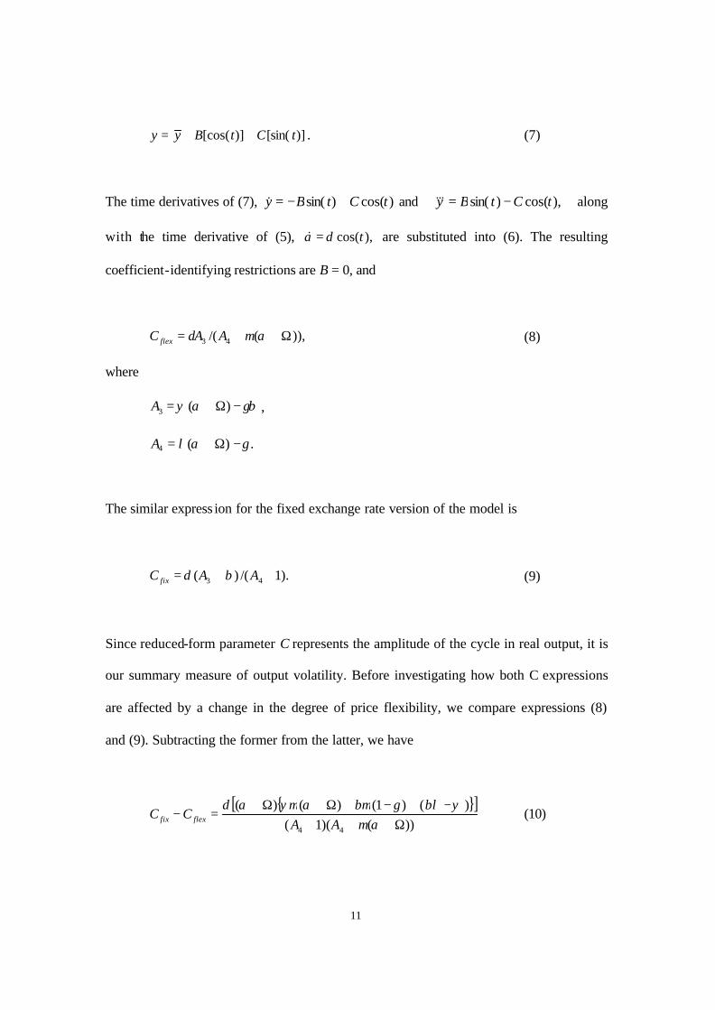
)][sin()][cos( tCtByy ++= . (7)

The time derivatives of (7), )cos()sin( tCtBy +−=& and ),cos()sin( tCtBy −=&&& along

with the time derivative of (5), ),cos(ta δ=& are substituted into (6). The resulting

coefficient-identifying restrictions are B = 0, and

)),(/( 43 Ω++= αµδ AAC flex (8)

where

γβαψ −Ω+= )(3A ,

.)(4 γαλ −Ω+=A

The similar express ion for the fixed exchange rate version of the model is

).1/()( 43 ++= AAC fix βδ (9)

Since reduced-form parameter C represents the amplitude of the cycle in real output, it is

our summary measure of output volatility. Before investigating how both C expressions

are affected by a change in the degree of price flexibility, we compare expressions (8)

and (9). Subtracting the former from the latter, we have

[ ]

))()(1()()1()()(

44 Ω+++−+−+Ω+Ω+

=−αµ

ψβλγβµαψµαδAA

CC flexfix (10)

12

The reader can verify that a sufficient, though not necessary, condition for 4A to be

positive is that intermediate imports be less than half of GDP. Assuming this to be true,

expression (10) is positive as long as .0)( >−ψβλ The illustrative parameter values

cited in the previous section indicate that this condition is certainly satisfied. We

conclude that – as long as the degree of price flexibility is not affected by exchange rate

policy – the model supports a flexible exchange rate. In addition, it is worthwhile to note

that under a flexible exchange rate regime nominal income targeting outperforms price

level targeting. Table 1 reports the quantitative results when the degree of price

stickiness (τ ) is 0.75.

Table 1: Output effects --- Baseline Parameters

Amplitude of Ongoing Output cycles

Flexible exchange rate Fix exchange rate

Price level targeting Nominal income targeting

Baseline

Model 0.102 0.027 0.178

We now investigate the effect of changing price flexibility directly. We do so by re-

interpreting the slope coefficients of the “new” Phillips curve as *,σλλ = *σγγ = and

*,σψψ = where ,/)1( 2 ττσ −= ,1)/1()/2(* −+= αθλ ))1/(()/(* φφαγ −−Ω= and

./* αβψ = We differentiate both the C expressions with respect to σ. Since a higher σ

corresponds to an increased degree of price flexibility, we interpret a finding of

13

0/ >∂∂ σC as support for Keynes’ concern that more price flexibility increases the

amplitude of the ongoing cycle in real output.

For the case of flexible exchange rates (expression (8)), σ∂∂ /C is given as:

[ ][ ]2)())(

))((

Ω++−Ω+

−Ω+=

∂∂

∗∗

∗∗

αµσγασλ

βγψαµδσC

(11)

For the parameter values noted above, this expression must be positive, and the model

unambiguously supports Keynes’ concern; increased price flexibility must accentuate

output volatility. Two comments on this result are warranted. First, it is appealing on

intuitive grounds that there is more support for Keynes’ concern in the new neoclassical

synthesis model, compared to what emerged from the corresponding “old” small open

economy analysis. This is because Keynes’ concern is based on the presumption that the

de-stabil izing effect of the expected inflation/deflation rate dominates the stabilizing

effect of one-time changes in the price level. Since the “new” approach involves agents

that are more forward-looking, it makes sense that the de-stabilizing effect matters more.

The second point worth noting is that the analysis supports central banks that have taken

pride in the fact that their low-inflation, flexible exchange rate policy has decreased the

degree of nominal price flexibility. The analysis says that both dimensions of this policy

(the flexible exchange rate and the lower degree of price flexibility) help to lower output

volatility.

With a fixed exchange rate (expression (9)), σ∂∂ /C is given as:

14

[ ]

[ ]21)(

))((

+−Ω+

−Ω+=

∂∂

∗∗

∗∗

σγασλ

βλψαδσC

(12)

This expression must be negative if .0)( >− ∗∗ ψβλ This is the same condition that is

important for determining a preference for one exchange rate regime or the other – if a

direct effect of exchange rate policy on the degree of price flexibility is ignored. At first

glance, the analysis appears not to support European countries that have opted for

currency union, since the almost certainly satisfied 0)( >−ψβλ condition suggests that

a flexible exchange rate involves lower output volatility. But policy makers in these

countries have argued that, without the stability offered by a flexible rate, there will be

increased incentive for their citizens to accept structural reforms. If this prediction turns

out to be true, and if a decreased degree of price rigidity is one of the outcomes of this

general move toward flexibility, then this same condition, ,0)( >−ψβλ is sufficient for

the model to support this view. Thus, there is internal consistency within both views

about exchange rate policy. European policy makers appear to believe that Keynes’

concern is not applicable in a fixed exchange rate setting, and they are right; Others, such

as the Canadian authorities, appear to believe that Keynes’ conjecture is applicable in a

flexible exchange rate setting, and they are correct as well. As an illustration, Table 2

reports the results when the degree of price stickiness decreases from 0.75 to 0.50.

Table 2: Output effects --- Parameters with increased price flexibility

Amplitude of Ongoing Output cycles

Flexible exchange rate Fix exchange rate

Price level targeting Nominal income targeting

Baseline

Model 0.102 0.066 0.142

15

4)- Sensitivity Test --- Endogenous Persistence

In this section we explore “hybrid” IS and Phillips curve relationships. Fuhrer (2000) and

Amato and Laubach (2001) have pointed out that the standard Ramsey type Euler

Equation for consumption (which gives rise to an IS-type relationship) fails to capture the

dynamics of the aggregate output. Fuhrer (2000) allow for habit formation in preferences

while maintaining the assumption of optimal consumption choice on the part of

consumers. Amato and Laubach (2001), on the other hand, introduce the ‘rule of thumb’

behaviour on the part of a fraction of the household; the remaining fraction of the

household is able to optimize their consumption in a usual fashion. Their modification to

the standard consumer problem is justified on the grounds that it is costly to reoptimize

every period. Both these modifications, introducing habit persistence and incorporating ‘

rule of thumb behaviour’, leads to a lagged output gap term with some positive weight in

the IS equation.

Similarly, it has been pointed out by many researchers that ‘the new Keynesian Phillips

curve’ based on Calvo’s (1983) sticky price model generates inertia in the price level and

not the inflation rate and that this is inconsistent with stylized facts on inflation dynamics.

The empirical evidence (for example, Nelson (1998)) indicates that inflation responds

sluggishly to economic shocks. The ‘new Keynesian Phillips curve’ implies that inflation

is determined by the current output gap and current expectations of future inflation.

Inflation is, therefore, very flexible and responds immediately to monetary policy shocks

and hence does not accord with stylized facts. In order to capture the inflation persistence

16

found in the data, it is common to augment the basic forward-looking inflation

adjustment equation with the addition of lagged inflation. Fuhrer and Moore (1995) is

one such example. Mankiw and Reis (2001) suggest an alternative approach, which

departs from the assumption of sticky prices and replaces it with that of sticky

information. Empirical research of Gali and Gertler (1999) and Fuhrer (1997) have

generally found that when lagged inflation is added to the basic ‘new Keynesian Phillips

curve’, its coefficient is statistically and economically significant.

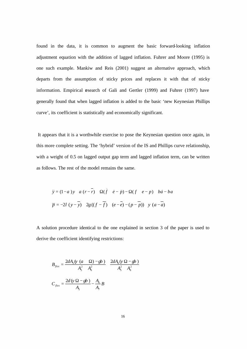
It appears that it is a worthwhile exercise to pose the Keynesian question once again, in

this more complete setting. The ‘hybrid’ version of the IS and Phillips curve relationship,

with a weight of 0.5 on lagged output gap term and lagged inflation term, can be written

as follows. The rest of the model remains the same.

aapefpefrryy ββαα −+−+Ω−−+Ω+−+−= &&&&&& )()()()1(

)())()()((2)(2 aappeeffyyp −+−−−+−+−−= ψγλ&&&

A solution procedure identical to the one explained in section 3 of the paper is used to

derive the coefficient identifying restrictions:

26

25

626

25

5 )(2))((2AA

AAA

ABflex +

−Ω+

+−Ω+

=γβψδγβαψδ

BAA

AC flex

7

6

5

)(2−

−Ω=

γβψδ

17

where,

)())2((25 Ω+−Ω−−= αµλαγA

)(26 Ω+−Ω= αλµA

The similar expressions for the fixed exchange rate case are quite messy so we do not

report them here. Instead, we just provide in table 3 the quantitative results of the

calibrated version of the model. Also, note that unlike the previous analysis the reduced-

form parameter B is not equal to zero. This means that the parameter C does not

independently represent the amplitude of the cycle in real output and thus cannot be

treated as a summary measure of output volatility.

Table 3: Output effects --- Baseline Parameters

Amplitude of Ongoing Output cycles

Flexible exchange rate Fix exchange rate

Price level targeting Nominal income targeting

Hybrid

Model 0.113 0.061 0.389

Table 4 provides the results with increased price flexibility, i.e., when τ = 0.5. While the

hybrid version of the model supports the initial conclusions in the flexible exchange rate

case, an interesting result emerges in the fix exchange rate case. The output volatility

does not go down with increased price flexibility, as was the case in the base line model.

18

Table 4: Output effects --- Parameters with increased price flexibility

Amplitude of Ongoing Output cycles

Flexible exchange rate Fix exchange rate

Price level targeting Nominal income targeting

Baseline

Model 0.113 0.105 0.421

5)- Conclusions

This note has used the new neoclassical synthesis model to reconsider Keynes’ concern

that an increased degree of price flexibility may increase output volatility. Earlier open-

economy analyses of this question involved models with less complete micro-foundations

and less forward-looking agents. Our results indicate that the reconsideration has been

worthwhile. The earlier research found only limited support for Keynes’ proposition

overall, with somewhat higher support under fixed exchange rates. With the new

analysis, which gives additional emphasis to forward-looking expectations, we find much

stronger support for Keynes’ proposition. Indeed, it must apply under flexible exchange

rates – the very policy regime that Keynes highlighted when drawing attention to his

concern.

We find two things reassuring. First, since we are uncomfortable with the proposition that

real-world policy makers are completely irrational, we find it appealing that the new

neoclassical synthesis model can identify the internal consistency that was noted in the

19

previous section. According to the model, those who favour fixed exchange rates are

correct when they expect that increased price flexibility will lower output volatility. Also

according to the model, those who favour flexible exchange rates and a domestic

monetary policy that focuses on price stability are correct when they argue that decreased

price flexibility will lower output volatility. Second, since we are uncomfortable with the

proposition that Keynes had bad intuit ion, we find it appealing that the macro framework

that has more reliable underpinings supports his conjecture that the de -stabilizing effect

of higher price flexibility is only likely to emerge under flexible exchange rates. As noted

in the introduction, traditional rational-expectations macro policy analysis could provide

neither of these reassurances.

While we find the results of this preliminary exploration encouraging, we stress the

value of further investigation. For one thing, it would be worth modeling the rest of the

world. In this note, we have assumed a cycle in demand for the domestic economy’s

exports (presumed to reflect an unexplained business cycle in the rest of the world). But

if that cycle were modeled, it is likely that there would be a corresponding cycle in both

the foreign interest rate and the foreign price level. To proceed along this line, the

domestic economy would have to involve an extension (such as overlapping generations)

so the rate of time preference of individual domestic agents (a constant) could differ from

the world interest rate (a variable following a cyclical time path). We hope that the

present note stimulates others to join us in pursuing these further analyses.

20

References

1)- Amato, J.D., and T. Laubach, (2001), “Rule-of-Thumb Behaviour and Monetary

Policy”, Unpublished Manuscript.

2)- Calvo, G., (1983), “Staggered Prices in a Utility Maximizing Framework”, Journal of

Monetary Economics, pp. 383-398.

3)- Chadha, B., (1988), “Is Increased Price Inflexibility Stabilizing?” IMF Working

Paper.

4)- Delong, B., and L. Summers, (1986), “Is Increased Price Flexibility Stabilizing?,

American Economic Review 76, pp. 1031 – 1044.

5)- Devereux, M., (2001), “Monetary Policy, Exchange Rate Flexibility, and Exchange

Rate Pass-through”, in “Revisiting the Case for Flexible Exchange Rates”, Bank of

Canada, Forthcoming.

6)- Devereux, M, amd C. Engel, (2001), “Exchange Rate Pass -through, Exchange Rate

Volatility, and Exchange Rate Disconnect”, Unpublished Manuscript.

7)- Driskill, R., and S. Sheffrin, (1986), “Is Price Flexibility Destabilizing?” American

Economic Review 76, pp. 802 – 807.

8)- Flemming, J.S., (1987), “Wage Flexibility and Employment Stability”, Oxford

Economic Papers 39, pp. 161- 174.

9)- Fuhrer, J.C., (1997), “Towards a Compact, Empirically Verified Rational

Expectations Model for Monetary Policy Analysis”, Carnegie -Rochester Conference

Series on Public Policy 47, pp. 197 – 230.

21

10)- Fuhrer, J.C., and G. Moore, (1995), “Inflation Persistence”, Quarterly Journa l of

Economics 110, pp. 127 – 159.

11)- Gali, J., and M. Gertler, (1999), “Inflation Dynamics: A Structural Econometric

Analysis”, Journal of Monetary Economics 44, pp. 195 – 222.

12)- Howitt, P., (1986), “Wage Flexibility and Employment”, Eastern Economic Journal

12, pp. 237 – 242.

13)- Keynes, J.M., (1936), “General Theory of Employment, Interest and Money”,

McMillan, London.

14)- King, S.R., (1988), “Is Increased Price Flexibility Stabilizing?: Comment”,

American Economic Review 78, pp. 267 – 272.

15)- King, R.G. (2000), “The New IS-LM Model: Language, Logic, and Limits”,

Economic Quarterly, Federal Reserve Bank of Richmond, Vol. 86, No.3, pp. 45 – 103.

16)- Mankiw, N.G., and R. Reis, (2001), “Sticky Information versus Sticky Prices: A

Proposal to Replace the New Keynesian Phillips Curve”, NBER Working Paper No.

8290.

17)- McCallum, B., and E. Nelson, (1999b), “An Optimizing IS-LM Specification for

Monetary Policy and Business Cycle Analysis”, Journal of Money, Credit and Banking,

pp. 296-316.

18)- McCallum, B., and E. Nelson, (2001), “Monetary Policy for an Open Economy: An

Alternative Framework with Optimizing Agentsand Sticky Prices”, Oxford Review of

Economic Policy, Vol. 16, No. 4.

22

19)- Myers, G., and W. Scarth, (1990), “Is Price Flexibility Destabilizing? Evidence for

the Open Economy”, Journal of International Economics 28, pp. 349 – 363.

20)- Sargent, T.J., and N. Wallace, (1981), “Rational Expectations and the Theory of

Economic Policy”, Journal of Monetary Economics 2, pp. 169 – 183.