IS-LM Equilibrium

Prof. Lutz Hendricks

Econ520

February 28, 2017

1 / 38

Objectives

In this section you will learn how to

1. put IS and LM together and derive the equilibrium;2. determine the effects of shocks and policies on equilibrium

output and interest rate

2 / 38

Model Summary

I Endogenous objects: Y, iI Exogenous objects: I,c0,G,T

I also M, which we take as controlled by CB for now

I Equations:I IS: Y = C(Y−T) + I(Y, i) + GI LM: M/P = YL(i)

3 / 38

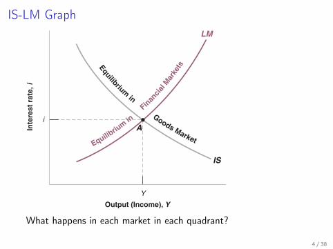
IS-LM GraphLM

IS

A

Output (Income), YY

Inte

rest

rat

e, i

i

Equilibriu

m in

Finan

cial M

arke

ts Equilibrium in Goods Market

What happens in each market in each quadrant?

4 / 38

Applications

Increasing Taxes

Y

i

IS

LM

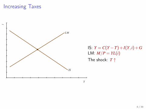
IS: Y = C(Y−T) + I(Y, i) + GLM: M/P = YL(i)

The shock: T ↑

6 / 38

Taxes and Investment

I A common argument:I higher taxes reduce disposable income and savingI saving = investmentI investment must fall

I Another common argument:I higher taxes reduce the government deficitI more money available for investment

I Which argument is right?

7 / 38

Increasing Taxes

What is missing in our analysis?

8 / 38

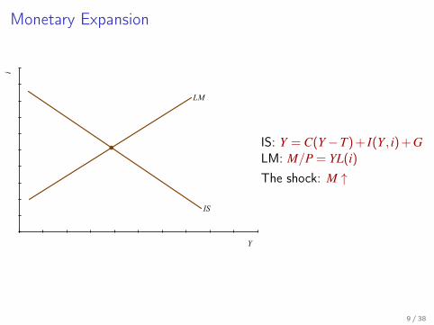
Monetary Expansion

Y

i

IS

LM

IS: Y = C(Y−T) + I(Y, i) + GLM: M/P = YL(i)

The shock: M ↑

9 / 38

Policy Mix

I By combining monetary and fiscal policy, the government can,in principle, move Y and i independently.

I Monetary expansion: Y ↑, i ↓I Fiscal expansion: Y ↑, i ↑I Combination: Y ↑, i unchangedI In a typical recession, monetary and fiscal policies expand

10 / 38

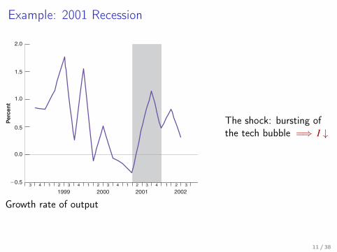
Example: 2001 RecessionP

erce

nt

1999

2.0

1.5

1.0

0.5

0.0

!0.5 1 2 3 4 1 2 3 4 1 2 3 4 1 2 33 4

2000 2001 2002

Growth rate of output

The shock: bursting ofthe tech bubble =⇒ I ↓

11 / 38

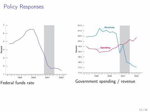
Policy ResponsesP

erce

nt

7

6

5

4

3

2

1

19993 4 1 2 3 4 1 2 3 4 1 2 3 4 1 2 3

2000 2001 2002

Federal funds rate

Per

cent

21.5

21.0

20.5

20.0

19.5

19.0

18.5

18.0

17.5

17.0

Revenues

Spending

19993 4 1 2 3 4 1 2 3 4 1 2 3 4 1 2 3

2000 2001 2002

Government spending / revenue

12 / 38

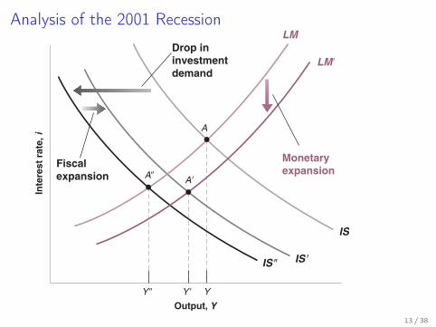
Analysis of the 2001 Recession

IS

Output, YYY!

Inte

rest

rat

e, i

IS "

LM!

LMDrop ininvestmentdemand

Monetaryexpansion

IS !

A!

A

Y "

A"Fiscalexpansion

13 / 38

Liquidity Traps

I Why do monetary policies have such a hard time pulling Japanout of recession?

I Real interest rates near zeroI Suggests flat LM curveI “Liquidity trap”

14 / 38

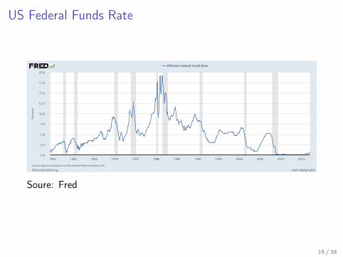
US Federal Funds Rate

myf.red/g/czDx

0.0

2.5

5.0

7.5

10.0

12.5

15.0

17.5

20.0

1955 1960 1965 1970 1975 1980 1985 1990 1995 2000 2005 2010 2015

fred.stlouisfed.orgSource:BoardofGovernorsoftheFederalReserveSystem(US)

EffectiveFederalFundsRate

Percent

Soure: Fred

15 / 38

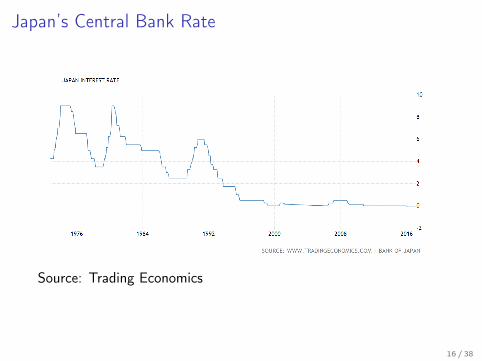
Japan’s Central Bank Rate

Source: Trading Economics

16 / 38

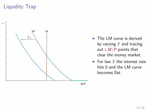
Liquidity Trap

M/P

i

MsMd

Y ↓ I The LM curve is derivedby varying Y and tracingout i,M/P points thatclear the money market.

I For low Y the interest ratehits 0 and the LM curvebecomes flat.

17 / 38

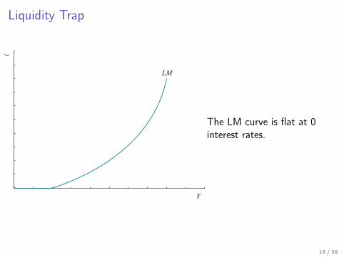
Liquidity Trap

Y

i

LM

The LM curve is flat at 0interest rates.

18 / 38

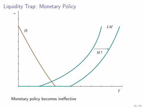
Liquidity Trap: Monetary Policy

Y

i

LMIS

M ↑

Monetary policy becomes ineffective19 / 38

Policy options in a liquidity trap

If the interest rate is zero, what can the Fed do?

20 / 38

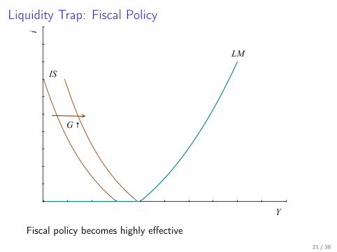
Liquidity Trap: Fiscal Policy

Y

i

LM

IS

G ↑

Fiscal policy becomes highly effective21 / 38

A Few Major Caveats

The IS-LM model makes the government look too powerful.

I By raising G it can achieve any level of Y.I When is this a reasonable shortcut?

It looks like saving lowers output.

I What is missing?

22 / 38

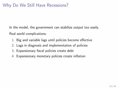
Why Do We Still Have Recessions?

In the model, the government can stabilize output too easily.

Real world complications:

1. Big and variable lags until policies become effective2. Lags in diagnosis and implementation of policies3. Expansionary fiscal policies create debt4. Expansionary monetary policies create inflation

23 / 38

An important point to remember

The IS-LM model makes strong assumptions: fixed prices, elasticsupply, government can borrow without cost.When applying the model, you need to consider how theseassumptions modify the results.(Or build a more comprehensive model)

Adding Banks

Adding Banks

In the IS/LM model, the Fed looks very powerful.

I it controls i and thus investment.

In reality, the behavior of banks can undo monetary policy actions.

26 / 38

The role of banks

Banks take in deposits and turn them into loans.A fraction of the deposits is held as CB reserves.Reserves provide bank liquidity.The Fed requires banks to hold about 10% of their deposits inreserves.

27 / 38

Adding Banks

Why do banks matter for monetary policy?

Suppose the Fed increases the supply of money.

I this is vague for now (how the Fed actually do this?)

Typically, this increases the amount of loans banks make, whichdrives down i.In some situations, banks absorb the additional money withoutcreating additional loans.

I they increase their CB reservesI then monetary policy has no power to lower interest rates

I example: 2008 financial crisis

28 / 38

The Money Multiplier

Money = currency + checkable deposits (+ perhaps other stuff)

I M = CU + D

The Fed does not directly control M.It controls high powered money H

I supplied as currency CU or reserves central bank R.

How do we get from H to M?

I the answer is: via bank lending

29 / 38

Bank lending

In principle, banks could make loans of unlimited size.In practice, the reserve requirement limits bank lending

The Fed requires that banks hold fraction θ of their deposits in aFed account.Only the remainder can be lent out.

R≥ θD (1)

Typically, θ ≈ 0.1.Of course, banks may hold larger reserves: θ ≥ θ

30 / 38

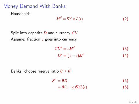
Money Demand With BanksHouseholds:

Md = $Y×L(i) (2)

Split into deposits D and currency CU.Assume: fraction c goes into currency

CUd = cMd (3)

Dd = (1− c)Md (4)

Banks: choose reserve ratio θ ≥ θ :

Rd = θD (5)= θ(1− c)$YL(i) (6)

31 / 38

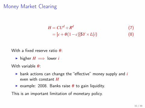
Money Market Clearing

H = CUd + Rd (7)= [c + θ(1− c)]$Y×L(i) (8)

With a fixed reserve ratio θ :

I higher H =⇒ lower i

With variable θ :

I bank actions can change the “effective” money supply and ieven with constant H

I example: 2008. Banks raise θ to gain liquidity.

This is an important limitation of monetary policy.

32 / 38

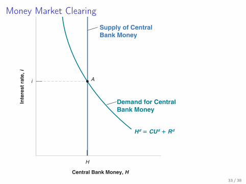
Money Market Clearing

H

A

Hd ! CUd " Rd

Central Bank Money, H

Demand for CentralBank Money

Supply of CentralBank Money

Inte

rest

rat

e, i

i

33 / 38

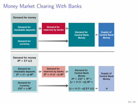
Money Market Clearing With Banks

Demand for money

Demand for checkable deposits

Demand for reserves by banks

Demand for Central Bank

Money

Supply of Central Bank

MoneyDemand for

currency

!

Demand for moneyMd ! $Y L(i)

Demand for checkable deposits

Dd ! (1"c) Md

Demand for reserves by banksRd ! (1"c) Md

Demand for Central Bank

MoneyHd ! CUd # Rd !

[c # (1"c)] Md !

[c # (1"c)] $Y L(i )

Supply of Central Bank

Money

H

Demand for currency

CUd ! c Md !

$

$

$

34 / 38

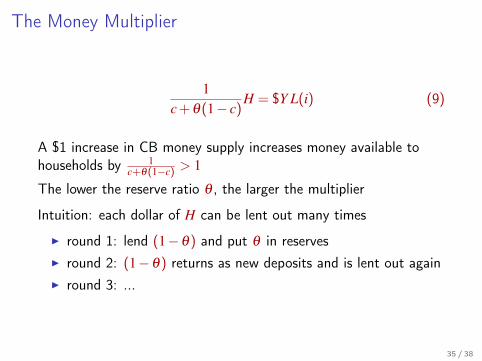
The Money Multiplier

1c + θ(1− c)

H = $Y L(i) (9)

A $1 increase in CB money supply increases money available tohouseholds by 1

c+θ(1−c) > 1

The lower the reserve ratio θ , the larger the multiplier

Intuition: each dollar of H can be lent out many times

I round 1: lend (1−θ) and put θ in reservesI round 2: (1−θ) returns as new deposits and is lent out againI round 3: ...

35 / 38

The Fed Funds Rate

Long ago, changing the reserve requirement θ was an importanttool of monetary policy

I this is no longer the case

Today, the main monetary policy tools is the Federal Funds Rate

I Banks lend reserves to each other over night at the Fed FundsRate

I The Fed controls the FFR tightly by choosing available reserves

The mechanism:

I H ↓=⇒ R ↓=⇒ i ↑I again, the complication is that banks may reduce θ which

dampens the effect on i

36 / 38

Reading

Blanchard and Johnson (2013), ch. 5 and 9.2On how the Fed works:

I Johnson, Manuel (2002). “Federal Reserve System.” TheLibrary of Economics and Liberty: a very brief overview of howthe Fed operates.

I Monetary Policy Basics: a brief summary of fed operations.I Labonte and Makinen (2017): A more detailed description

(including unconventional monetary policy).

37 / 38

References I

Blanchard, O. and D. Johnson (2013): Macroeconomics, Boston:Pearson, 6th ed.

Labonte, M. and G. E. Makinen (2017): “Monetary policy and theFederal Reserve: current policy and conditions,” CongressionalResearch Service, Library of Congress.

38 / 38