Is Interaction Necessary for Distributed Private Learning?

Adam Smith∗, Abhradeep Thakurta†, Jalaj Upadhyay∗∗School of Electrical Engineering and Computer Science,

Pennsylvania State University, Email: asmith, jalaj@psu.edu†Department of Computer Science, University of California Santa Cruz,

Email: aguhatha@ucsc.edu

Abstract—Recent large-scale deployments of differen-tially private algorithms employ the local model forprivacy (sometimes called PRAM or randomized response),where data are randomized on each individual’s devicebefore being sent to a server that computes approximate,aggregate statistics. The server need not be trusted forprivacy, leaving data control in users’ hands.

For an important class of convex optimization prob-lems (including logistic regression, support vector ma-chines, and the Euclidean median), the best known locallydifferentially-private algorithms are highly interactive,requiring as many rounds of back and forth as there areusers in the protocol.

We ask: how much interaction is necessary to optimizeconvex functions in the local DP model? Existing lowerbounds either do not apply to convex optimization, or saynothing about interaction.

We provide new algorithms which are either nonin-teractive or use relatively few rounds of interaction. Wealso show lower bounds on the accuracy of an importantclass of noninteractive algorithms, suggesting a separationbetween what is possible with and without interaction.

Keywords-Differential privacy, local differential privacy,convex optimization, oracle complexity.

I. INTRODUCTION

Each of us generates vast quantities of data as weinteract with modern networked devices. Accurate ag-gregate statistics about those data can generate valuablebenefits to society—higher quality healthcare, moreefficient systems and lower power consumption, amongothers. However, those data are highly sensitive, paint-ing detailed pictures of our lives. Private data analysis,broadly, seeks to enable the benefits of learning fromthese data without exposing individual-level informa-tion. Differential privacy [17] is a rigorous privacycriterion for data analysis that provides meaningfulguarantees regardless of what an adversary knows aheadof time about individuals’ data [25]. Differential privacyis now widely studied and algorithms satisfying thecriterion are increasingly deployed [1, 2, 19].

There are two well-studied models for implementingdifferentially-private algorithms. In the central model,raw data are collected at a central server where they

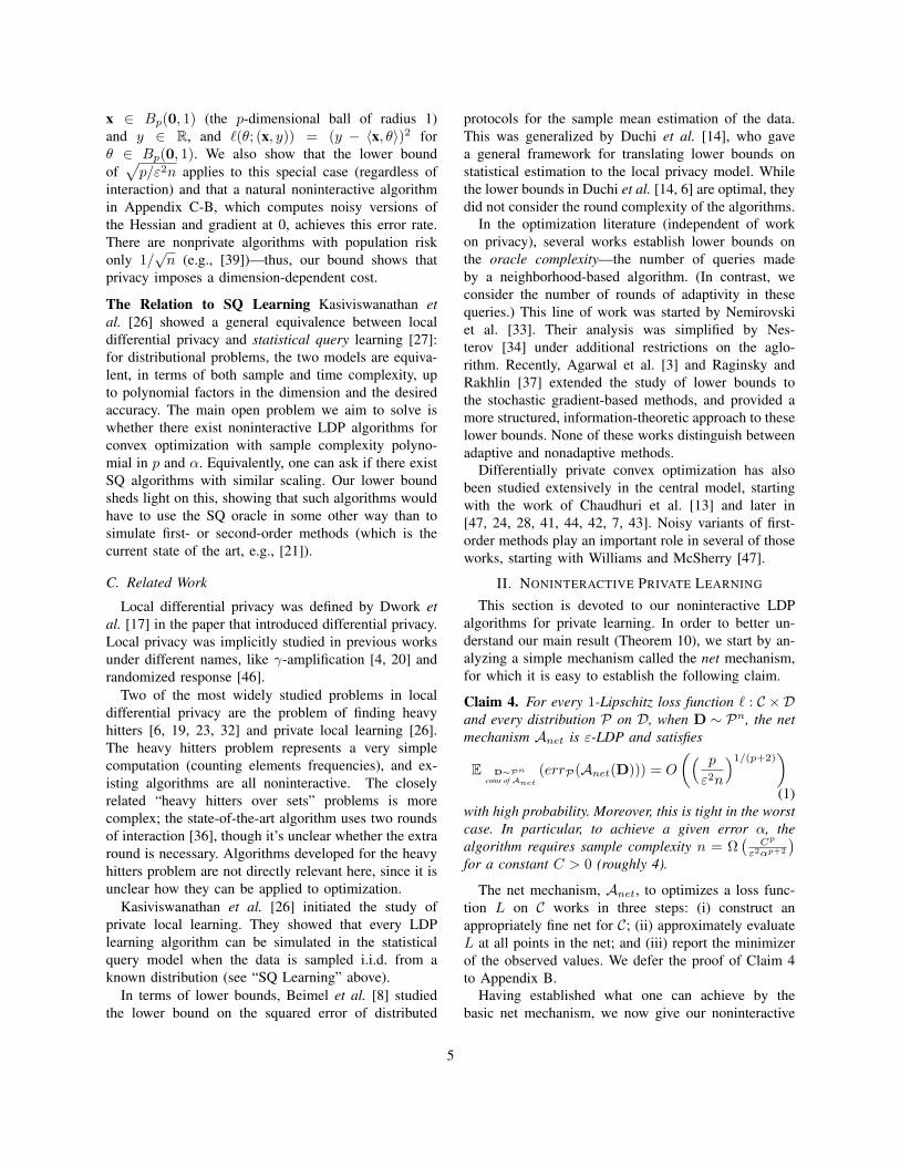
are processed by a differentially-private algorithm. Inthe local model [20] (dubbed LDP and illustrated inFigure 1), each individual applies a differentially-privatealgorithm locally to their data and shares only theoutput of the algorithm—called a report or response—with a server that aggregates users’ reports. The localmodel allows individuals to retain control of their datasince privacy guarantees are enforced directly by theirdevices. However, it entails a different set of algorithmictechniques from the central model. In principle, onecould also use cryptographic techniques such as securefunction evaluation to simulate central model algo-rithms in a local model, but such algorithms currentlyimpose bandwidth and liveness constraints that makethem impractical for large deployments. For example,Google [19] now collects certain usage statistics fromusers’ devices subject to local differential privacy; thosealgorithms are run by hundreds of millions of users.

A long line of work studies what is achievable byLDP algorithms, and tight upper and lower boundsknown on the achievable accuracy for many problems;see Sec. I-C. For a large class of optimization problems,however, the algorithms that achieve the upper boundare highly interactive—the server exhanges messagesback and forth in sequence with each user in the system(see Figure 1). Implementing interactive protocols forprivate data collection is difficult, because networklatency introduces delays and because the server mustbe live throughout the protocol. Consequently, existinglarge-scale deployments [19] are limited to noninterac-tive algorithms.

The question naturally arises: how much power islost by restricting to noninteractive protocols? Ka-siviswanathan et al. [26] studied the role of interactionin locally private algorithms, exhibiting a problem thatcan be solved using a linear (in the dimension) amountof data by a 2-round protocol but for any noninteractiveprotocol requires an exponential-sized data set. Theproblem they study is somewhat unatural, based onlearning parity functions; their results say little about thecomputations commonly carried out in machine learning

or statistical analysis.

Contributions. This paper initiates the study of inter-action in local differential privacy (LDP) for importantand natural learning problems. Specifically, we focus onconvex optimization, which encompasses the calculationof descriptive statistics, such as the median, as well asmore sophisticated computations, such as fitting linearor logistic regression models, training support vectormachines and sparse regression. Tight upper and lowerbounds are known for the accuracy of LDP convexoptimization [14]. However, the upper bounds are highlyinteractive, requiring as many rounds of back and forthas there are users in the protocol.

We provide new algorithms for noninteractiveLDP optimization of convex Lipschitz functions overa bounded parameter space. These algorithms im-prove considerably over naıve approaches. For one-dimensional problems (e.g., median), our algorithmsattain the same optimal error bounds as interactivesolutions. For higher-dimensional problems, our algo-rithms’ error guarantees are worse than the boundsfor interactive algorithms, since our guarantees decayexponentially as the dimension increases (instead ofpolynomially).

We provide evidence that this exponential dependenceis necessary. We show lower bounds on the error ofa natural class of nonadaptive optimization algorithms,which includes the noninteractive LDP variants of first-order methods such as gradient descent. This lowerbound applies even to nonprivate algorithms. It demon-strates that the adaptivity of first- and second-ordermethods is necessary to get a polynomial dependenceon the dimension.

We also consider algorithms that use interaction onlysparingly. We show that carefully tuned LDP variants of

Users

zi s

……

Q1

Qi

Qn

Server

Analysts

z1

zn

d1

di

dn

random string

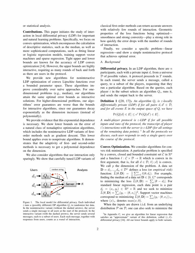
Figure 1. The local model for differential privacy. Each individuali runs a (possibly different) DP algorithm Qi to randomize her data.In the noninteractive variant (without the dashed arrows), the serversends a single message to all users at the start of the protocol. In theinteractive variant (with the dashed arrows), the server sends severalmessages, each to a subset of users. Each such message, together withresponses from users, counts as a round of interaction.

classical first-order methods can return accurate answerswith relatively few rounds of interaction. Geometricproperties of the loss functions being optimized—smoothness and strong convexity—play a strong role inhow quickly the error drops with the number of roundsof interaction.

Finally, we consider a specific problem—linearregression—and show a simple noninteractive protocolthat achieves optimal error.

A. Background

Differential privacy. In an LDP algorithm, there are nparticipants, each with a private input di from a universeD of possible values. A protocol proceeds in T rounds.In each round, the server sends a message, called aquery, to a subset of the players, requesting that theyrun a particular algorithm. Based on the queries, eachplayer i in the subset selects an algorithm Qi, runs it,and sends the output back to the server.

Definition 1 ([20, 17]). An algorithm Qi is ε-locallydifferentially private (LDP) if for all pairs d, d′ ∈ D,and for all events E in the output space of Q, we have

Pr[Q(d) ∈ E] ≤ eε Pr[Q(d′) ∈ E] .

A multi-player protocol is ε-LDP if for all possibleinputs and runs of the protocol, the transcript of playeri’s interactions with the server is ε-LDP (for all settingsof the remaining data points). 1 In all the protocols wediscuss, each user responds to only a single query overthe course of the protocol.

Convex Optimization. We consider algorithms for con-vex risk minimization. A particular problem is specifiedby a convex, closed and bounded constraint set C in Rpand a function ` : C × D → R which is convex in itsfirst argument, that is, for all d ∈ D, `(·; d) is convex.We call p the dimension of the problem. A data setD = d1, ..., dn ∈ Dn defines a loss (or empirical risk)function: L(θ;D) = 1

n

∑ni=1 `(θ; di). For example,

finding the median of a data set D ∈ [0, 1]n correspondsto minimizing the loss L(θ,D) =

∑i |θ − di|. For

standard linear regression, each data point is a pairdi = (xi, yi) ∈ Rp × R and we seek to minimizeL(θ,D) =

∑i(yi − 〈θ, xi〉)2. Support vector machines

correspond to minimizing L(θ,D) =∑i(yi · 〈θ, xi〉)+,

where (x)+ denotes max(x, 0).When the inputs are drawn i.i.d. from an underlying

distribution P on D, one can also seek to minimize the

1In Appendix C, we give an algorithm for linear regression thatsatisfies an “approximate” variant of this definition, called (ε, δ)-differential privacy [16]. All our lower bounds apply to both variants.

2

population risk, or generalization error, defined as theexpected error on a fresh example from the distribution:LP(θ) = ED∼P [`(θ;D)] . We drop the subscript Pwhen it is clear from the context.

We state the error of our algorithms in terms of theirexcess (empirical or population) risk. Given an outputθpriv ∈ C, we define two variants of excess risk.

Empirical: errD(θpriv) = L(θpriv;D)−minθ∈C

L(θ;D)

Population: errP(θpriv) = LP(θpriv)−minθ∈C

LP(θ) .

The empirical error measures how well our output doeson the data set at hand. The population error assumesthe data is drawn from some distribution, and measureshow well our algorithm does on unseen examples fromthe same distribution. The measures are closely related,but not the same (roughly, algorithms that “overfit” mayhave low empirical error but high population error).

We consider additional restrictions on the loss func-tion `. Ignoring the second argument for a moment,we say a function ` : C → R is L-Lipschitz if forall θ, θ′ ∈ C, |`(θ) − `(θ′)| ≤ L‖θ − θ′‖2 . (Unlessotherwise specified, we work with the `2 norm on Rp.)We say ` is ∆-strongly convex if, for every θ, θ′ ∈ Cand for every subgradient ∇`(θ) ∈ ∂`(θ), we have`(θ′) ≥ 〈∇`(θ), θ′ − θ〉 + 1

2∆2‖θ′ − θ‖22. We say `is β-smooth if it is differentiable and has β-Lipschitzgradients, that is ‖∇`(θ)−∇`(θ′)‖2 ≤ β‖θ − θ′‖2 .

Nonprivate methods for optimizing convex functionsgenerally use first- or second-order methods, which gaininformation about the loss funcion by evaluating thegradient, and possibly the Hessian (matrix of secondderivatives) at a sequence of points in C. Examples ofsuch methods include gradient descent, cutting planealgorithms, Frank-Wolfe, and Newton-Raphson.

“Typical” Setting. In what follows, we assume C ⊂ Rpis a convex set (‖C‖2 ≤ 1) and ` : C×D → R is convexand 1-Lipschitz for each setting of its second argument.For this setting, Duchi et al. [14] gave an n-roundalgorithm with expected population risk O

(√pε2n

),

where n is the number of users. Their algorithm is aLDP version of stochastic gradient descent where, atround i, the server sends the current estimate θi to playeri, who returns a noisy gradient Q(∇`(θi; di)) (whereQ adds carefully calibrated noise). They also showedthat error bound is tight, using an information theoreticargument. The lower bound applies even to linear lossfunctions—in particular, the bound shows that assumingsmoothness does not change the achievable error.

B. Summary of Results

Noninteractive Algorithms for General Convex Op-timization.

Theorem 2 (Theorem 10, informal). For the typicalsetting above, there is an ε-LDP algorithm A suchthat for all distributions P on D, with high probability,

errP(A(D)) = O

(( √p

ε2n

)1/(p+1)), where O(·) hides

log(n) factors.

For one-dimensional convex optimization, our proto-col nearly matches the lower bound of Ω(1/

√ε2n). The

dependence on the dimension is exponential, however.To achieve a given level of error α, one requiresn ≥ Ω(cpε−2α−(p+1)) data points.

Our one-dimensional algorithm is based on a novelreduction of the general one-dimensional convex op-timization to the median problem (a special case),followed by a noninteractive local algorithm for themedian that uses a tree-based technique for simultane-ously approximating 1D range queries (that arises in[22, 18, 12]). For higher dimensions, we reduce to theone-dimensional case by optimizing, in parallel, overa collection of roughly 1/αp−1 random lines passingthrough the center of C.

As a comparison point, the most straightforward ap-proach to noninteractive LDP optimization is to evaluatethe loss function at all points in a suitably defined set(a “net”) for C, and then output the one with smallestloss. This approach incurs error O

((pε2n

)1/(p+2))

(or

alternatively, requires a sample of size 4pε−2α−(p+2)

for error α). Our technique saves a factor of 1/α in thesample complexity, which is significant for small α.

Bounds on Adaptivity for General Convex Optimiza-tion. We show that for a natural class of LDP methods,the exponential dependence on p in our methods is nec-essary. We start from the observation that methods forgeneral convex optimization, private or not, generallyaccess the loss function by approximating the gradientat a sequence of adaptively chosen points. We modelsuch algorithms by imagining an oracle to which thealgorithm makes queries. The oracle is neighborhood-based (usually called local2) if, on query θ ∈ C, itreturns information about the values of the loss functionin an infinitesimal neighborhood of θ (a subgradient orHessian, for example).

We study, for the first time, the adaptivity of suchalgorithms: suppose that the algorithm submits queries

2This use of “local” is completely different from its use in “localdifferential privacy”. We use “neighborhood-based” for clarity.

3

in batches to the oracle, with the choice of points in abatch depending only on query answers from previousbatches. A nonadaptive algorithm uses only one batch(and corresponds to a nointeractive LDP protocol). Weshow that for every noninteractive neighborhood-basedoracle algorithm requires (1/α)Ω(p) queries in the worstcase to obtain error α for optimizing Lipschitz convexfunctions:

Theorem 3 (Theorem 13, informal). There exists C > 0such that for every sufficiently small α > 0 and every(not necessarily private) neighborhood-based oracleO·(·), every C log(1/α)-round randomized algorithmfor optimization of Lipschitz convex functions requires2Ω(p) queries to succeed with high probability. Fur-thermore, nonadaptive algorithms require (1/α)Ω(p)

queries.

This is the first lower bound to demonstrate that theadaptivity of first-order methods such as gradient de-scent and the cutting-plane method is in fact necessaryto get a polynomial dependence on the dimension. Italso demonstrates that fundamentally new techniqueswould be necessary to get noninteractive LDP algo-rithms with polynomial dependence on the dimension.Previous bounds on oracle optimization [3, 34, 33, 37]used information-theoretic arguments that do not distin-guish between adaptive and nonadaptive algorithms (inparticular, the instances that arise in those proofs areeasy to solve nonadaptively).

Algorithms with Limited Adaptivity. Although thedesign of accurate noninteractive algorithms for high-dimensional optimization remains challenging, we showthat LDP algorithms with limited interaction can achievelow error, demonstrating that the n rounds of interactionof previous algorithms (where n is the number of users)are not necessary. These algorithms are noisy, “batchstochastic” versions of two classic first-order methods—gradient descent and the cutting plane method—wherein each round many users are queried to get high-accuracy estimates of the gradient at a particular point.We show:

1) In the “typical” setting (optimizing 1-Lipschitzfunctions over a bounded set) then for everyT , there is an ε-LDP algorithm A(·) suchthat for every D ∈ Dn, E[errD(A(D))] =

O(

min(√

Tnε2 +

(1− 1

e

)T/p, 1√

T+√

pε2n

)).

In particular, this algorithm achieves optimal errorO(√p/ε2n) for T = nε2/p (due to the second

term). On the other hand, the first term reachesthe optimal error when T = O(p log(ε2n/p)).

2) When the function is 1-Lipschitz, β-smooth and

Assumptions Method Additive Error(big-Oh expression)

1-Lipschitz GD 1√T+√

pnε2

1-Lipschitz CP

√Tnε2 + 2

(1− 1

e

)T/p∆-strongly convex GD 1

∆T + pnε2∆

β-smooth GD 1T 2 +

pT 2

nε2β

β-smooth, GDβ2e−∆T/β + pT 2

nε2

∆-strongly convex

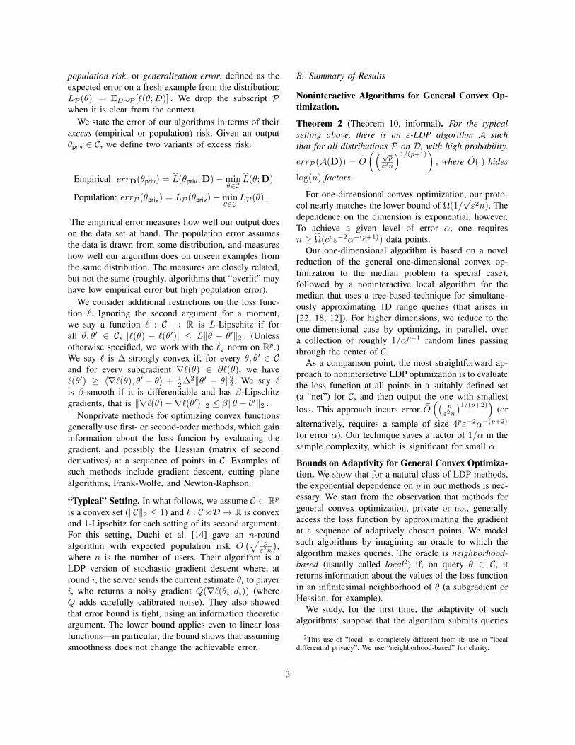
Figure 2. Upper bounds on achievable error for optimization of 1-Lipschitz convex functions in the local model as a function of thenumber T of rounds of interaction, the number n of users, and thedimension p of the parameter vector. Methods: GD = gradient descent,CP = cutting plane.

∆-strongly convex, there is an ε-LDP algorithmA(·) that for every D ∈ Dn,E[errD(A(D))] = O

(β2 e−∆T/β + pT 2

nε2

). Our

algorithm requires both smoothness and strongconvexity to achieve this bound, and our anal-ysis requires a new analysis of batch stochasticgradient descent under these conditions. The roleof smoothness is surprising: without restrictionson interaction, assuming strong convexity helpswith accuracy, but adding smoothness does not.However, smoothness is known to accelerate theconvergence of gradient descent, and that translatesinto a much better dependency on T in our con-text.3

Note. We state all our results in expectation, but theyalso extend to high probability guarantee using the ideaof Bassily et al. [7, Appendix D].

Case Study: Linear Regression Our work also raisesthe question of what can be achieved for specificproblems. In Appendix C-A, we study the accuracy ofnoninteractive LDP protocols for ordinary least squaresregression, where each input d is a pair (x, y) with

3One can show that if the loss function is 1-Lipschitz and β-smooth, then the ε-LDP algorithm version of batch stochastic gradientdescent can be tuned (using Lan’s analysis [29]), so that for everyD ∈ Dn, E[errD(A(D))] = O

(1T2 + pT2

nε2β

). This achieves op-

timal error O(√p/ε2n) for T = (nε2/p)1/4, which is quadratically

faster than the case when the function is 1-Lipschitz. Similarly, onecan also show (using [40]) that if the loss function is 1-Lipschitzand ∆-strongly convex, then ε-LDP batch SGD satisfies, for everyD ∈ Dn, E[errD(A(D))] = O

(1

∆T+ pnε2∆

). For constant ∆,

this achieves very low error O(p/ε2n) when T = (nε2/p)—thesame number of rounds, but much lower error than, what one getsfrom Lipschitz continuity alone.

4

x ∈ Bp(0, 1) (the p-dimensional ball of radius 1)and y ∈ R, and `(θ; (x, y)) = (y − 〈x, θ〉)2 forθ ∈ Bp(0, 1). We also show that the lower boundof√p/ε2n applies to this special case (regardless of

interaction) and that a natural noninteractive algorithmin Appendix C-B, which computes noisy versions ofthe Hessian and gradient at 0, achieves this error rate.There are nonprivate algorithms with population riskonly 1/

√n (e.g., [39])—thus, our bound shows that

privacy imposes a dimension-dependent cost.

The Relation to SQ Learning Kasiviswanathan etal. [26] showed a general equivalence between localdifferential privacy and statistical query learning [27]:for distributional problems, the two models are equiva-lent, in terms of both sample and time complexity, upto polynomial factors in the dimension and the desiredaccuracy. The main open problem we aim to solve iswhether there exist noninteractive LDP algorithms forconvex optimization with sample complexity polyno-mial in p and α. Equivalently, one can ask if there existSQ algorithms with similar scaling. Our lower boundsheds light on this, showing that such algorithms wouldhave to use the SQ oracle in some other way than tosimulate first- or second-order methods (which is thecurrent state of the art, e.g., [21]).

C. Related Work

Local differential privacy was defined by Dwork etal. [17] in the paper that introduced differential privacy.Local privacy was implicitly studied in previous worksunder different names, like γ-amplification [4, 20] andrandomized response [46].

Two of the most widely studied problems in localdifferential privacy are the problem of finding heavyhitters [6, 19, 23, 32] and private local learning [26].The heavy hitters problem represents a very simplecomputation (counting elements frequencies), and ex-isting algorithms are all noninteractive. The closelyrelated “heavy hitters over sets” problems is morecomplex; the state-of-the-art algorithm uses two roundsof interaction [36], though it’s unclear whether the extraround is necessary. Algorithms developed for the heavyhitters problem are not directly relevant here, since it isunclear how they can be applied to optimization.

Kasiviswanathan et al. [26] initiated the study ofprivate local learning. They showed that every LDPlearning algorithm can be simulated in the statisticalquery model when the data is sampled i.i.d. from aknown distribution (see “SQ Learning” above).

In terms of lower bounds, Beimel et al. [8] studiedthe lower bound on the squared error of distributed

protocols for the sample mean estimation of the data.This was generalized by Duchi et al. [14], who gavea general framework for translating lower bounds onstatistical estimation to the local privacy model. Whilethe lower bounds in Duchi et al. [14, 6] are optimal, theydid not consider the round complexity of the algorithms.

In the optimization literature (independent of workon privacy), several works establish lower bounds onthe oracle complexity—the number of queries madeby a neighborhood-based algorithm. (In contrast, weconsider the number of rounds of adaptivity in thesequeries.) This line of work was started by Nemirovskiet al. [33]. Their analysis was simplified by Nes-terov [34] under additional restrictions on the aglo-rithm. Recently, Agarwal et al. [3] and Raginsky andRakhlin [37] extended the study of lower bounds tothe stochastic gradient-based methods, and provided amore structured, information-theoretic approach to theselower bounds. None of these works distinguish betweenadaptive and nonadaptive methods.

Differentially private convex optimization has alsobeen studied extensively in the central model, startingwith the work of Chaudhuri et al. [13] and later in[47, 24, 28, 41, 44, 42, 7, 43]. Noisy variants of first-order methods play an important role in several of thoseworks, starting with Williams and McSherry [47].

II. NONINTERACTIVE PRIVATE LEARNING

This section is devoted to our noninteractive LDPalgorithms for private learning. In order to better un-derstand our main result (Theorem 10), we start by an-alyzing a simple mechanism called the net mechanism,for which it is easy to establish the following claim.

Claim 4. For every 1-Lipschitz loss function ` : C ×Dand every distribution P on D, when D ∼ Pn, the netmechanism Anet is ε-LDP and satisfies

E D∼Pncoins of Anet

(errP(Anet(D))) = O

(( p

ε2n

)1/(p+2))(1)

with high probability. Moreover, this is tight in the worstcase. In particular, to achieve a given error α, thealgorithm requires sample complexity n = Ω

(Cp

ε2αp+2

)for a constant C > 0 (roughly 4).

The net mechanism, Anet, to optimizes a loss func-tion L on C works in three steps: (i) construct anappropriately fine net for C; (ii) approximately evaluateL at all points in the net; and (iii) report the minimizerof the observed values. We defer the proof of Claim 4to Appendix B.

Having established what one can achieve by thebasic net mechanism, we now give our noninteractive

5

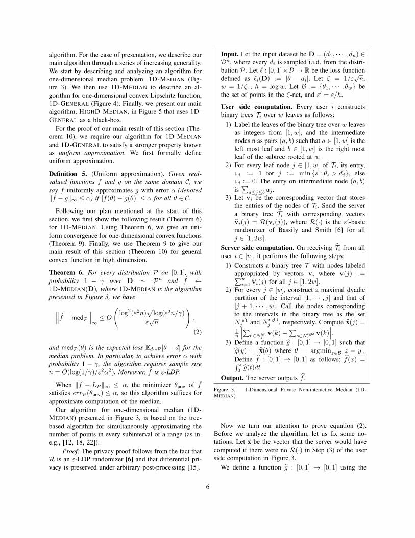
algorithm. For the ease of presentation, we describe ourmain algorithm through a series of increasing generality.We start by describing and analyzing an algorithm forone-dimensional median problem, 1D-MEDIAN (Fig-ure 3). We then use 1D-MEDIAN to describe an al-gorithm for one-dimensional convex Lipschitz function,1D-GENERAL (Figure 4). Finally, we present our mainalgorithm, HIGHD-MEDIAN, in Figure 5 that uses 1D-GENERAL as a black-box.

For the proof of our main result of this section (The-orem 10), we require our algorithm for 1D-MEDIANand 1D-GENERAL to satisfy a stronger property knownas uniform approximation. We first formally defineuniform approximation.

Definition 5. (Uniform approximation). Given real-valued functions f and g on the same domain C, wesay f uniformly approximates g with error α (denoted‖f − g‖∞ ≤ α) if |f(θ)− g(θ)| ≤ α for all θ ∈ C.

Following our plan mentioned at the start of thissection, we first show the following result (Theorem 6)for 1D-MEDIAN. Using Theorem 6, we give an uni-form convergence for one-dimensional convex functions(Theorem 9). Finally, we use Theorem 9 to give ourmain result of this section (Theorem 10) for generalconvex function in high dimension.

Theorem 6. For every distribution P on [0, 1], withprobability 1 − γ over D ∼ Pn and f ←1D-MEDIAN(D), where 1D-MEDIAN is the algorithmpresented in Figure 3, we have

∥∥∥f −medP

∥∥∥∞≤ O

(log2(ε2n)

√log(ε2n/γ)

ε√n

),

(2)

and medP(θ) is the expected loss Ed∼P |θ − d| for themedian problem. In particular, to achieve error α withprobability 1 − γ, the algorithm requires sample sizen = O(log(1/γ)/ε2α2). Moreover, f is ε-LDP.

When ‖f − LP‖∞ ≤ α, the minimizer θpriv of fsatisfies errP(θpriv) ≤ α, so this algorithm suffices forapproximate computation of the median.

Our algorithm for one-dimensional median (1D-MEDIAN) presented in Figure 3, is based on the tree-based algorithm for simultaneously approximating thenumber of points in every subinterval of a range (as in,e.g., [12, 18, 22]).

Proof: The privacy proof follows from the fact thatR is an ε-LDP randomizer [6] and that differential pri-vacy is preserved under arbitrary post-processing [15].

Input. Let the input dataset be D = (d1, · · · , dn) ∈Dn, where every di is sampled i.i.d. from the distri-bution P . Let ` : [0, 1]×D → R be the loss functiondefined as `i(D) := |θ − di|. Let ζ = 1/ε

√n,

w = 1/ζ , h = logw. Let B := θ1, · · · , θw bethe set of points in the ζ-net, and ε′ = ε/h.

User side computation. Every user i constructsbinary trees Ti over w leaves as follows:

1) Label the leaves of the binary tree over w leavesas integers from [1, w], and the intermediatenodes n as pairs (a, b) such that a ∈ [1, w] is theleft most leaf and b ∈ [1, w] is the right mostleaf of the subtree rooted at n.

2) For every leaf node j ∈ [1, w] of Ti, its entry,uj := 1 for j := min s : θs > dj, elseuj := 0. The entry on intermediate node (a, b)is∑a≤j≤b uj .

3) Let vi be the corresponding vector that storesthe entries of the nodes of Ti. Send the servera binary tree Ti with corresponding vectorsvi(j) = R(vi(j)), where R(·) is the ε′-basicrandomizer of Bassily and Smith [6] for allj ∈ [1, 2w].

Server side computation. On receiving Ti from alluser i ∈ [n], it performs the following steps:

1) Constructs a binary tree T with nodes labeledappropriated by vectors v, where v(j) :=∑ni=1 vi(j) for all j ∈ [1, 2w].

2) For every j ∈ [w], construct a maximal dyadicpartition of the interval [1, · · · , j] and that of[j + 1, · · · , w]. Call the nodes correspondingto the intervals in the binary tree as the setN leftj and N right

j , respectively. Compute x(j) =1n

∣∣∣∑n∈N leftj

v(k)−∑

n∈N rightj

v(k)∣∣∣.

3) Define a function g : [0, 1] → [0, 1] such thatg(y) = x(θ) where θ = argminz∈B |z − y|.Define f : [0, 1] → [0, 1] as follows: f(x) =∫ x

0g(t)dt

Output. The server outputs f .

Figure 3. 1-Dimensional Private Non-interactive Median (1D-MEDIAN)

Now we turn our attention to prove equation (2).Before we analyze the algorithm, let us fix some no-tations. Let x be the vector that the server would havecomputed if there were no R(·) in Step (3) of the userside computation in Figure 3.

We define a function g : [0, 1] → [0, 1] using the

6

vector x similar to the definition of the function g(·),i.e., g(y) = x(θ) where θ = argminz∈B |z − y|.

In what follows, we first prove that for all θ ∈ B,

‖g(θ)− g(θ)‖∞ ≤ O

(log2(ε2n)

√log(ε2n/γ)

ε√n

)(3)

Our analysis uses the observation that, every level ofthe binary tree T (i.e., the corresponding entries of thevector v) can be seen as a noisy histogram (over the datauniverse B) of the user’s data and, by the definition ofthe vector x, the vector x succinctly stores the estimatesof ∇medP at different net points.

Let γ′ = γ/h. Since the data universe has size w =ε√n, we can use Theorem 2.3 of Bassily and Smith [6]

to estimate the `∞-error in estimating ∇medP at everylevel k ∈ [h]. Bassily and Smith [6, Theorem 2.3] givesthat, with probability 1− γ′, the `∞ error in estimating

∇medP is at most O(

1ε

√log(w/γ′)

n

)for every level

k ∈ [h]. Using union bound over all the levels, we have

maxθ∈B|g(θ)− g(θ)| = O

(h

ε′

√log(w/γ′)

n

)By substituting ε′ = ε/h, h = logw, and setting w =ε√n, we get equation (3).

We now return to proving Theorem 6. From thedefinition of f and equation (3), we have the followingset of inequalities for all x ∈ [0, 1]:

|f(x)−medP(x)| =∫ x

0

∣∣g(θ)−∇medP(θ)∣∣dθ

≤dx/ζe−1∑t=1

∫ (t+1)ζ

tζ

∣∣(g(θ)−∇medP(θ))∣∣ dθ

≤

dx/ζe∑t=1

αζ

+ ζ(∇med(1)−∇med(0))

≤ α+ 2ζ = O(

log2(ε2n)√

log(ε2n/γ)/(ε√n))

,

where α denotes the left-hand side in Equation (3). Thelast inequality follows from the fact that the summationis over at most w = 1/ζ net points and that med is1-Lipschitz. This completes the proof of Theorem 6.

We now proceed to the general one-dimensionalconvex function. We first state the following key lemma.

Lemma 7. Let f : [0, 1] → [0, 1] be a convex 1-Lipschitz function. Then there exists a distribution Qsuch that

∀θ ∈ [0, 1], f(θ) = Ey∼Q[|θ − y|] + c

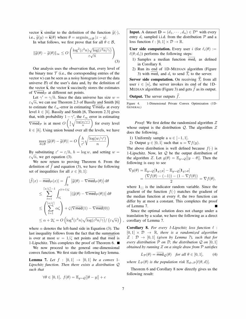
Input. A dataset D = (d1, · · · , dn) ∈ Dn with everyentry di sampled i.i.d. from the distribution P and aloss function ` : [0, 1]×D → R.

User side computation. Every user i (for `i(θ) :=`(θ; di)) performs the following steps:

1) Samples a median function medi as definedin Corollary 8.

2) Run its end of 1D-MEDIAN algorithm (Figure3) with medi and di to send Ti to the server.

Server side computation. On receiving Ti from alluser i ∈ [n], the server invokes its end of the 1D-MEDIAN algorithm (Figure 3) and gets f as its output.

Output. The server outputs f .

Figure 4. 1-Dimensional Private Convex Optimization (1D-GENERAL)

Proof: We first define the randomized algorithm Zwhose output is the distribution Q. The algorithm Zdoes the following.

1) Uniformly sample a u ∈ [−1, 1].2) Output y ∈ [0, 1] such that u = ∇f(y).

The above distribution is well defined because f(·) is1-Lipschitz. Now, let Q be the output distribution ofthe algorithm Z. Let g(θ) = Ey∼Q[|y − θ|]. Then thefollowing is easy to see

∇g(θ) = Ey∼Q[1y≤θ]− Ey∼Q[1y>θ]

=(∇f(θ)− (−1))− (1−∇f(θ))

2= ∇f(θ),

where 1[·] is the indicator random variable. Since thegradient of the function f(·) matches the gradient ofthe median function at every θ, the two function candiffer by at most a constant. This completes the proofof Lemma 7.

Since the optimal solution does not change under atranslation by a scalar, we have the following as a directcorollary of Lemma 7.

Corollary 8. For every 1-Lipschitz loss function ` :[0, 1] × D → R, there is a randomized algorithmZ : D → [0, 1] (given by Lemma 7), such that forevery distribution P on D, the distribution Q on [0, 1]obtained by running Z on a single draw from P satisfies

LP(θ) = medQ(θ) for all θ ∈ [0, 1], (4)

where LP(θ) is the population risk Ed∼P [`(θ, d)].

Theorem 6 and Corollary 8 now directly gives us thefollowing result:

7

Theorem 9. Let ` : [0, 1] × D → R be a 1-Lipschitzloss function such that `( 1

2 , d) = 0 for all d ∈ D. Forevery distribution P on P , with probability 1− γ overD ∼ Pn and f ← 1D-GENERAL(D, `), where 1D-GENERAL(·, ·) is the algorithm presented in Figure 4,we have∥∥∥f − LP∥∥∥

∞≤ O

(log(ε2n)

√log(ε2n/γ)

ε√n

),

and LP(θ) is the population risk ED∼P(`(θ,D)). Inparticular, to achieve error α with probability 1−γ, thealgorithm requires sample size n = O(log(1/γ)/ε2α2).

The above theorem basically shows that we canuniformly approximate any 1-Lipschitz convex functiondefined over R. This observation is crucial for ouralgorithm in the high dimensional case.

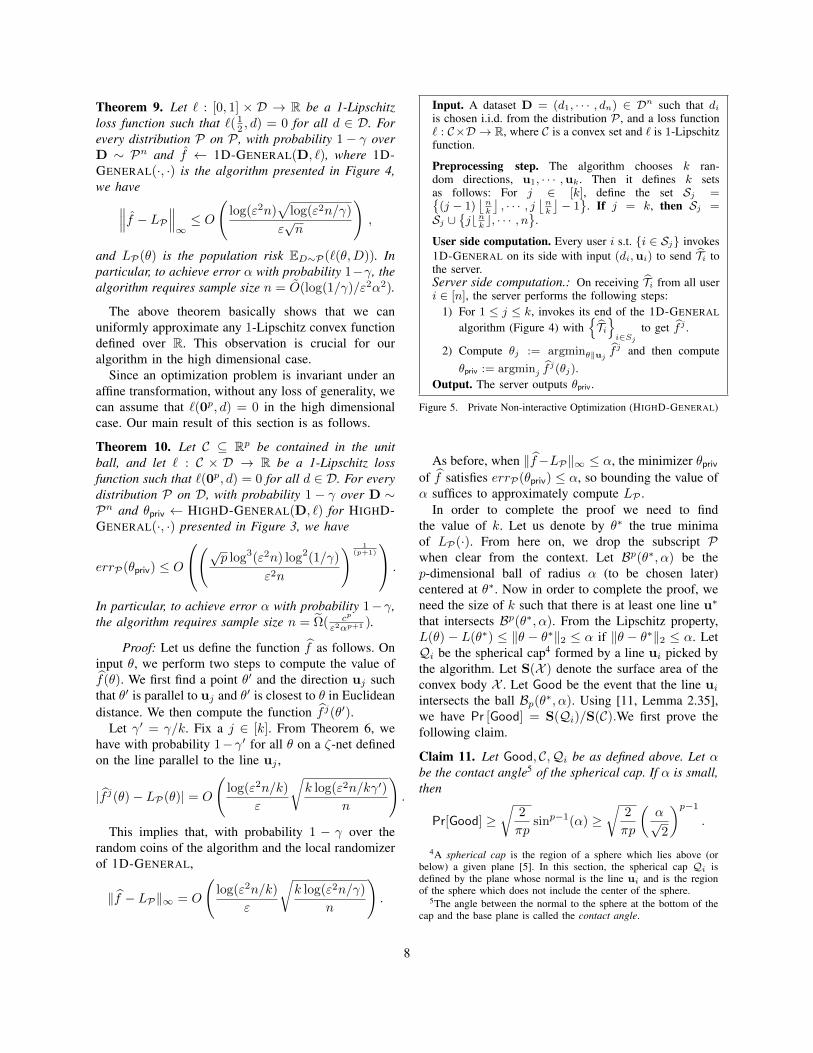
Since an optimization problem is invariant under anaffine transformation, without any loss of generality, wecan assume that `(0p, d) = 0 in the high dimensionalcase. Our main result of this section is as follows.

Theorem 10. Let C ⊆ Rp be contained in the unitball, and let ` : C × D → R be a 1-Lipschitz lossfunction such that `(0p, d) = 0 for all d ∈ D. For everydistribution P on D, with probability 1 − γ over D ∼Pn and θpriv ← HIGHD-GENERAL(D, `) for HIGHD-GENERAL(·, ·) presented in Figure 3, we have

errP(θpriv) ≤ O

(√p log3(ε2n) log2(1/γ)

ε2n

) 1(p+1)

.

In particular, to achieve error α with probability 1−γ,the algorithm requires sample size n = Ω( cp

ε2αp+1 ).

Proof: Let us define the function f as follows. Oninput θ, we perform two steps to compute the value off(θ). We first find a point θ′ and the direction uj suchthat θ′ is parallel to uj and θ′ is closest to θ in Euclideandistance. We then compute the function f j(θ′).

Let γ′ = γ/k. Fix a j ∈ [k]. From Theorem 6, wehave with probability 1−γ′ for all θ on a ζ-net definedon the line parallel to the line uj ,

|f j(θ)− LP(θ)| = O

(log(ε2n/k)

ε

√k log(ε2n/kγ′)

n

).

This implies that, with probability 1 − γ over therandom coins of the algorithm and the local randomizerof 1D-GENERAL,

‖f − LP‖∞ = O

(log(ε2n/k)

ε

√k log(ε2n/γ)

n

).

Input. A dataset D = (d1, · · · , dn) ∈ Dn such that diis chosen i.i.d. from the distribution P , and a loss function` : C×D → R, where C is a convex set and ` is 1-Lipschitzfunction.

Preprocessing step. The algorithm chooses k ran-dom directions, u1, · · · ,uk. Then it defines k setsas follows: For j ∈ [k], define the set Sj =(j − 1)

⌊nk

⌋, · · · , j

⌊nk

⌋− 1

. If j = k, then Sj =Sj ∪

jbn

kc, · · · , n

.

User side computation. Every user i s.t. i ∈ Sj invokes1D-GENERAL on its side with input (di,ui) to send Ti tothe server.Server side computation.: On receiving Ti from all useri ∈ [n], the server performs the following steps:

1) For 1 ≤ j ≤ k, invokes its end of the 1D-GENERAL

algorithm (Figure 4) withTii∈Sj

to get f j .

2) Compute θj := argminθ‖uj fj and then compute

θpriv := argminj fj(θj).

Output. The server outputs θpriv.

Figure 5. Private Non-interactive Optimization (HIGHD-GENERAL)

As before, when ‖f−LP‖∞ ≤ α, the minimizer θprivof f satisfies errP(θpriv) ≤ α, so bounding the value ofα suffices to approximately compute LP .

In order to complete the proof we need to findthe value of k. Let us denote by θ∗ the true minimaof LP(·). From here on, we drop the subscript Pwhen clear from the context. Let Bp(θ∗, α) be thep-dimensional ball of radius α (to be chosen later)centered at θ∗. Now in order to complete the proof, weneed the size of k such that there is at least one line u∗

that intersects Bp(θ∗, α). From the Lipschitz property,L(θ)− L(θ∗) ≤ ‖θ − θ∗‖2 ≤ α if ‖θ − θ∗‖2 ≤ α. LetQi be the spherical cap4 formed by a line ui picked bythe algorithm. Let S(X ) denote the surface area of theconvex body X . Let Good be the event that the line uiintersects the ball Bp(θ∗, α). Using [11, Lemma 2.35],we have Pr [Good] = S(Qi)/S(C).We first prove thefollowing claim.

Claim 11. Let Good, C,Qi be as defined above. Let αbe the contact angle5 of the spherical cap. If α is small,then

Pr[Good] ≥√

2

πpsinp−1(α) ≥

√2

πp

(α√2

)p−1

.

4A spherical cap is the region of a sphere which lies above (orbelow) a given plane [5]. In this section, the spherical cap Qi isdefined by the plane whose normal is the line ui and is the regionof the sphere which does not include the center of the sphere.

5The angle between the normal to the sphere at the bottom of thecap and the base plane is called the contact angle.

8

Proof: Using the sine rule, we have α cos(α/2) =sinα Using the fact that sin2 α + cos2 α = 1 andcosα = 2 cos2(α/2) − 1, rearranging the expressiongives us

α√2

=

√1− cos2 α

1 + cosα=√

1− cosα. (5)

In particular, this implies that cosα = 1 − α2

2 .Therefore,

Pr[Good] ≥√

2

πpsinp−1(α)

=

√2

πp

(1−

(1− α2

2

)2)1/(p−1)

≥√

2

πp

αp−1

2(p−1)/2.

This completes the proof of Claim 11.If we set k = O

(2(p−1)/2 log(1/γ)

αp−1

√πp2

),

then Claim 11 implies that there exists an j ∈ [k] suchthat, with probability 1 − γ, uj intersects Bp(θ∗, α).Substituting this value of k in equation (5), we get

‖f − LP‖∞ = O

log(1/γ)

ε

√log3(ε2n)

√p2p−2

nαp−1

.

Setting α = O

(( √p

ε2n log3(ε2n) log2(1/γ))1/(p+1)

),

we get ‖f − LP‖∞ ≤ α. This completes the proofof Theorem 10.

In particular, to achieve a given error α, the theoremstates that the algorithm HIGHD-GENERAL requiressample complexity n = Ω( cp

ε2αp+1 ) for a constant c > 0(roughly 2).

III. ROUND COMPLEXITY OF ADAPTIVEALGORITHMS USING NEIGHBORHOOD ORACLES

In this section, we show that, for a natural class ofalgorithms, the exponential dependence on the dimen-sion is essential. We first define the basic model andthen state our result. We assume that an algorithm hasan access to a special kind of oracle which we calla neighborhood-based oracle and can make queries inbatches, where queries in a particular batch may dependon the queries and response from previous batches.

Neighborhood-based oracles. We assume that the al-gorithm has access to an oracle OF (·) for a convexfunction F : C → [0, 1], where C ⊆ Rp is a convex setover which the function is defined. We say the oracle isneighborhood-based (also called local, see the footnote

on page 3) if, given θ ∈ C, the oracle outputs a valuethat depends on the function F (·) and the infinitesimalneighborhood of the query point θ. For example, onesuch query can be to compute the h-th order gradient,∇hF (θ), at the point θ.

Query model. We assume that the algorithm is random-ized and can make at most q queries in T batches, wherebatch-i consists of qi queries such that

∑Ti=1 qi = q.

We call any such algorithms that makes at most qqueries in T -batches a (q, T )-adaptive algorithm if, forall 1 ≤ i ≤ T − 1, the queries in the (i + 1)-th batchdepends only on the queries made and the responsesreceived during the first i batches. When T = 1, wecall such algorithm a q-nonadaptive algorithm. Notethat our query model does not assume the queries madein a particular batch are independent, i.e., queries in asingle batch may have non-trivial correlation.

Our first claim shows that there exists a distributionover convex function defined on a convex set C ⊆ Rp,such that for a function F chosen from this distribution,any q-nonadaptive algorithm can outputs a θ∗ such thatF (θ∗)−minθ∈C F (θ) ≤ α/21 with probability at mostqαp. That is, to get a constant success probability, anynon-adaptive algorithm has to make number of queriesexponential in the dimension of the underlying convexset. More precisely, we show the following.

Theorem 12. Let Bp(0p, 1) denote a unit ball centeredaround the origin. There exists a distribution F ofconvex functions from Bp(0p, 1) to [0, 1] such that, forF ∼ F , the following holds:

1) Let OF (·) be a neighborhood based oracle for Fas defined above. Then the output θ∗ of any q-nonadaptive and randomized algorithm, with ora-cle access to OF (·), satisfies

Pr

[∣∣∣∣F (θ∗)− minθ∈Bp(0p,1)

F (θ)

∣∣∣∣ ≤ α/21

]≤ qαp.

2) There exists a (poly(log(1/α)), 2)-adaptive algo-rithm that can compute θ∗ with probability at least2/3, such that

∣∣F (θ∗)−minθ∈Bp(0p,1) F (θ)∣∣ ≤ α.

Remark 1. We first note the implication of this result inthe model of local-differential privacy. Theorem 12 rulesout any nonadaptive algorithms, including non-privatealgorithms, that just uses gradient information. This inparticular implies that there exists a convex functionfor which no local-differentially private algorithm, withaccess to neighborhood oracle, can output a θpriv suchthat errD(θpriv) ≤ α with high probability. In otherwords, it shows that adaptivity is necessary for gradient

9

based methods to achieve polynomial dependence on thedimension.

The idea behind of our proof is as follows. Recallthat we need to construct a distribution of functionsF such that a function sampled from F is hard tooptimized using only non-adaptive queries. We definea distribution F that satisfies the following properties:(i) the minimum of any function sampled from F liesin a uniformly at random chosen p-dimensional ball Bof radius α, (ii) any algorithm that makes neighborhoodqueries does not learn anything about the optimum pointunless it queries a point inside the ball B, and (iii) if analgorithm queries a point inside the ball, it learns theoptimum value. Once we have such a distribution offunction, we are basically done because the probabilitywith which any query point is a point inside a smallp-dimensional ball depends on the volume of B and thevolume of B decays exponentially with p.

We now return to proving Theorem 12.Proof of Theorem 12: Let C := c1, · · · , cN

be the centers of N balls that forms an α-packing ofBp(0p, 1). That is,

∀i ∈ [N ] and θ such that ‖θ − ci‖2 ≤ α, θ ∈ Bp(0p, 1)

∀i 6= j ∈ [N ], ‖ci − cj‖2 ≥ 2α.

Pick a point c ∈ C uniformly at random. Pick two pointsc ∈ Bp(0p, 1) and c ∈ Bp(0p, 1) such that α/6 ≤‖c−c‖2 ≤ α/3, α/6 ≤ ‖c−c‖2 ≤ α/3, and ‖c−c‖2 ≥2α/3. Define the following functions:

F0(θ) := max

‖θ − c‖2,

1

3‖θ − c‖2 +

1

3

F1(θ) := max

‖θ − c‖2,

1

3‖θ − c‖2 +

1

3

The function F is chosen by flipping a uniform coinb and setting F (θ) := Fb(θ). Since all three functionsf, f0, and f1 are convex function and point-wise max-imum of two convex functions is a convex function,both F0 and F1 are convex functions. Similarly, it iseasy to verify that the function F (θ) is 1-Lipschitz.Moreover, ∇F (θ) = 1 for all θ ∈ Bp(0p, 1)\Bp(c, α)and ∇F (θ) = 1/3 for all θ ∈ Bp(c, α).

We first enumerate some key properties of F0(·). Thesame properties holds for F1(·) as well. Let θ∗ :=argminθ∈Bp(c,α) F (θ). First note that F (c) = F0(c)if b = 0. That is the minimum of the function F isθ∗ = c when b = 0. Similarly, θ∗ = c when b = 1.

We fix a notation that we use very often in this proof.For a function G, let

disc(G; θ) :=

∣∣∣∣G(θ)− minθ∈Bp(0p,1)

G(θ)

∣∣∣∣ .

When b = 0, for all θ ∈ Bp(0p, 1) such thatdisc(F0; θ) ≤ α/21, we have ‖θ − c‖2 ≤ α/7. This isbecause of the construction of f0 and that the minimumof F0 occurs at θ = c. That is, for all such θ,

‖c− θ‖2 ≥ ‖c− c‖2 − ‖θ − c‖2 ≥α

6− α

7> 0

‖c− θ‖2 ≥ ‖c− c‖2 − ‖θ − c‖2 ≥2α

3− α

7>α

2.

Moreover, since ‖θ−c‖2 ≤ α/7, we have ‖θ−c‖2 ≤α/3 + α/7 < α. Therefore, all θ such that disc(F0; θ),we have θ ∈ Bp(c, α). Similarly, when b = 1, for allζ ∈ Bp(0p, 1) such that disc(F1; θ) ≤ α/21, we haveζ ∈ Bp(c, α), ‖c − ζ‖2 > 0, and ‖c − θ‖2 > α/2.The second and higher order derivative of the func-tion F is identically zero and the ∇F (θ) = 1 forall θ ∈ Bp(0p, 1)\Bp(c, α) and ∇F = 1/3 for allθ ∈ Bp(c, α).

This implies that in order to output whether θ∗ = c orθ∗ = c, at least one of the queries of any q-nonadaptivealgorithm has to be a point inside the ball Bp(c, α).Now fix a query i. Since the ratio of the volume ofball Bp(c, α) to the volume of Bp(0p, 1) is αp, theprobability that the query i is a point inside the ballis αp. By a union bound, the probability that any querylands in the ball is at most qαp, as desired.

To prove the second part of the claim, we show thatthere is an efficient adaptive algorithm Adaptive thatoutputs θ∗ such that disc(F ; θ∗) ≤ α. Adaptive makestwo batches of queries:

1) In the first batch, Adaptive randomly picks a pointθ ∈ Bp(0p, 1) and queries for the gradient ∇F (θ).

2) Let g be the direction of the gradient returned.In the second batch, Adaptive randomly pickspoly(log(1/α)) points in Bp(0p, 1) along the di-rection of g and makes gradient queries at all thesepoints in the second round.

By Chernoff bound, with probability at least 2/3, aquery in the second batch is a point that lies inBp(c, α). This allows the algorithm to output θ∗ suchthat disc(F ; θ∗) ≤ α. This completes the proof.

In the view of Theorem 12, a natural question arisesis whether, is it always possible to output a θ∗ usingconstant round of adaptivity and neighborhood oraclesfor a function F sampled from any arbitrary distributionF of functions defined over a convex set C, such thatdisc(F, θ∗) ≤ α? Our next result shows that this is nottrue in general. That is, there exists a distribution offunctions from Bp(0p, 1) to [0, 1], such that, for F (·)sampled from that distribution, no (poly(p), O(1))-adaptive (and randomized) algorithm with access toOF can output a θ∗ such that disc(F, θ∗) ≤ α with

10

a constant probability. More formally, we have thefollowing theorem.

Theorem 13. Let Bp(0p, 1) denotes a unit ball centeredaround the origin. There exists a distribution F ofconvex functions from a unit ball Bp(0p, 1) to [0, 1]such that, for F ∼ F , the following holds. Let OF (·) bea neighborhood based oracle for F as defined above.For every α > 0, there exists a T := T (α), withT (α) = Θ(log(1/α), such that the output θ∗ of any(q, T )-adaptive and randomized algorithm with oracleaccess to OF (·), satisfies

Pr

[∣∣∣∣F (θ∗)− minθ∈Bp(0p,1)

F (θ)

∣∣∣∣ ≤ α] ≤ (T + 1)q2−p

1− 3−p.

Proof: Let B0 = Bp(0p, 1) and r0 = 1. Recursivelyfor all level of recursion, i = 1, · · · , T, define thefollowing:

1) Define an packing Vi of the ball Bi−1 with ballsof radius ri := 1

2

(718

)i−1.

2) Pick a random ball from the packing Vi withcenter c(i). Set this ball as Bi for the next levelof recursion.

3) Randomly pick c(i)0 , c

(i)1 ∈ Bi such that (i) balls of

radius ri/6 with centers c(i)0 and c

(i)1 lies in Bi are

disjoint, (ii) ri/12 ≤ ‖c(i)−c(i)0 ‖2, ‖c(i)−c(i)

1 ‖2 ≤ri/6 and (iii) ‖c(i)

0 − c(i)1 ‖2 ≥ ri/3.

4) If all the conditions in step 3 are not satisfied, goback to step 2 and repeat.

We define two functions at every level of the recur-sion as follows:

f(i)0 :=

(4

7

)i‖θ − c

(i)0 ‖2 +

1

3+ri3

i−1∑j=1

(4

7

)jf

(i)1 :=

(4

7

)i‖θ − c

(i)1 ‖2 +

1

3+ri3

i−1∑j=1

(4

7

)j .

Set f(θ) = ‖θ − c(1)‖2. Now pick T random bitsb1, · · · , bT and set the function as follows:

F (θ) := max

f(θ),

f

(i)bi

(θ)Ti=1

. (6)

Claim 14. The function F (·) is convex.

Proof: First note that the two functions defined inevery levels of recursion are convex. Further, f(·) isconvex. Since point-wise maximum of convex functionsis convex, the claim follows.

We now return to the proof of Theorem 13. Withoutloss of generality, let us assume that all the randombits b1, · · · , bT are 0. We can make this assumption

because the functions at the same level sets are definedanalogously. We first prove the following structuralproperty of our function. The claim basically says thatin a small ball around the points chosen in step 3 abovein any level of recursion, F (·) is defined by only thefunctions at the lower level of recursion.

Claim 15. Let i be any index in [T ]. Then for everyθ in the ball of radius ri+1 := 1

2

(718

)iaround c

(i)0 ,

F (θ) = maxi≤j≤T

f

(j)0 (θ)

.

Proof: We prove the claim by induction.Base case. When i = 1, then we have for all θ ∈ B2,f(θ) = ‖θ − c(1)‖2 ∈ [1/12, 5/18]. However, byconstruction, f (1)

0 (θ) := 47‖θ− c

(1)0 ‖2 + 1

3 ∈ [1/3, 4/9].

Therefore, for all θ ∈ B2, F (θ) = max1≤j≤T

f j0

Tj=1

.

This completes the base case.Inductive case. Let us assume that for every θ

in the ball of radius ri+1 around c(i)0 , F (θ) =

maxi≤j≤T

f

(j)0 (θ)

. To prove the claim, we need

to prove that, for θ ∈ Bi+2 around c(i+1)0 , F (θ) =

maxi<j≤T

f

(j)0 (θ)

. From the induction hypothesis

we know that F (θ) = maxi≤j≤T

f j0 (θ)

in the ball

Bi. Since Bi+2 ⊆ Bi+1 by construction, we need to

show that f (i)(θ) ≤ maxf j0 (θ)

Tj=i+1

. Note that

f(i)0 (θ) and f

(i+1)0 (θ) grows linearly as the distance

of the point θ from c(i)0 with slope

(47

)iand

(47

)i+1,

respectively. Therefore, if we prove that f (i+1)0 (θ) ≥

f(i)0 (θ) at the boundary of the ball Bi+2 and at θ =

c(i+1)0 , we are done. At θ = c

(i+1)0 , we have

f(i)0 (θ) ≤

(4

7

)iri6

+1

3+ri3

i−1∑j=1

(4

7

)j

≤ 1

3+ri3

i∑j=1

(4

7

)j≤ f (i+1)

0 (θ).

For θ at the boundary of the ball Bi+2, we have

f(i)0 (θ) =

(4

7

)i‖θ − c

(i)0 ‖+

1

3+ri3

i−1∑j=1

(4

7

)j≤(

4

7

)i‖c(i+1)

0 − c(i)0 ‖2 +

(4

7

)i‖c(i+1)

0 − θ‖2

+1

3+ri3

i−1∑j=1

(4

7

)j≤(

4

7

)iri6

+

(4

7

)i‖c(i+1)

0 − θ‖2 = f(i+1)0 (θ).

11

This completes the proof that for every θ in the ball of

radius ri+1 around c(i+1)0 , F (θ) = max

f

(j)0 (θ)

Tj=i

and Claim 15 follows.One of the main corollaries of Claim 15 is that c(T )

0 =argminθ∈Bp(0p,1) F (θ). Another direct consequence ofthis structural theorem is that F (θ) is 1-Lipschitz.

Now suppose θ ∈ Bp(0p, 1) is such that disc(F ; θ) ≤27

(718

)T.We know that F (θ) = f

(T )0 (θ) in the ball of

radius 12

(718

)T. Since c

(T )0 = argminθ∈Bp(0p,1) F (θ),

we know that ‖θ − c(T )0 ‖2 ≤ 1

14

(718

)T ≤ ‖c(r−1)0 −

c(T )0 ‖2. Since balls of radius 1

2

(718

)Taround c

(T )0 and

c(T )1 are disjoint, this implies that any such θ is closer

to c(T )0 . In other words, for any algorithm to output a

θ such that disc(F ; θ) ≤ 27

(718

)T, it has to distinguish

where the minimizer is c(T )0 or c(T )

1 . That is, any suchalgorithm has to query for a point inside the ball BT inat least one of the T batches.

Now the adversary can compute the minimizer in lessthan T rounds if, in the batch-j query, one of its queriesis a point inside Bi for i ≥ j. Let Ei,j be such anevent. Then for i ≥ 1,Pr[Ei,j ] = qjvol(Bi)/vol(Bj) ≤q(

718

)(i−j)p. Therefore, the probability with which the

adversary succeeds in computing a minimizer in lessthan T rounds is

Pr

[T∨i=1

Ei

]≤ q

((1

2

)Tp+ T

(7

18

)Tp).

Setting T := Θ(log(1/α)) completes the proof.

IV. NOISY-GRADIENT BASED METHODS

In this section we give noisy versions of the gradientcomputation based algorithms to solve convex opti-mization. Before we present our noisy gradient basedmethod, we first provide an exposition of an algorithm(in Section IV-A), which we will use heavily in this andlater sections, for estimating the gradient (and also theloss) of the population risk L(θ) = Ed∼P [`(θ; d)] atany θ.

A. Locally Differentially Private (LDP) Function andGradient Oracles

Gradient oracle: For a given data set D =d1, · · · , dn drawn i.i.d. from the population distri-bution P , the objective is to estimate the gradientof L(θ) = Ed∼P [`(θ; d)] at a given θ, using localreports from n/T samples from D. Algorithm NOISY-GRADIENT-ORACLE is expected to be called to estimatethe gradient at T different θ’s (θ1, · · · , θT ) using T setsof n/T disjoint samples.

Input. Current partition number: t, number of par-titions: T , current model estimate: θcurrent, privacyparameter: ε, value flag: flag ∈ T,F, fixed model:θ0. Let D = d1, · · · , dn ∼ Pn be the data set,L(θ) = Ed∼P [`(θ; d)] is a 1-Lipschitz function.

Algorithm. Perform the following steps:1) Define St =

(t− 1)b nT c, · · · , tb

nT c − 1

. If

t = T , then St = St ∪tb nT c, · · · , n

.

2) The server sends θcurrent to all the users. Ev-ery user i s.t. i ∈ St does the following:Compute zi := Rε(∇`(θcurrent; di)) and zi :=Rε(`(θcurrent; di)−`(θ0; di)), whereRε(·) is therandomizer defined in Appendix A.

3) Compute Lossnoisy (t) = 1St∑i∈St

zi and

Gradnoisy (t) = 1St∑i∈St

zi.

4) If flag=F, return Gradnoisy (t) else return(Gradnoisy (t), Lossnoisy (t)).

Figure 6. Locally Noisy Gradient Oracle (NOISY-GRADIENT-ORACLE)

Privacy guarantee. The following theorem is immedi-ate from the privacy result of Duchi et al. [14].

Theorem 16. NOISY-GRADIENT-ORACLE is ε-LDP.

In particular, since differential privacy is preservedunder post-processing, all our algorithms in this sectionare ε-LDP. In the following, we state the followingutility guarantees for the algorithm NOISY-GRADIENT-ORACLE. We will use both the unbiasedness and theconcentration properties below heavily in the later al-gorithms (see Appendix A for a proof).

Theorem 17. Let D = d1, · · · , dn be drawn i.i.d.from the distribution P , and let L(θ) = Ed∼P [`(θ; d)].Then for a fixed partition number t ∈ [T ] and a θcurrent(independent of the data samples in t), the followingare true for Algorithm NOISY-GRADIENT-ORACLE.

1) Unbiasedness: E [Gradnoisy (t)] = ∇L(θcurrent).2) Bounded variance:

E[‖Gradnoisy (t)−∇L(θcurrent)‖22

]= O

(Tp/nε2

).

3) Tight concentration: Let x be any vector(with ‖x‖2 ≤ 1) independent of the sampleset St and the gaussian noise added in Fig-ure 6. Then with probability at least 1 − γ,|〈Gradnoisy (t), x〉 − 〈∇L(θcurrent), x〉| is boundedby O

(√T log(1/γ)/nε2

).

12

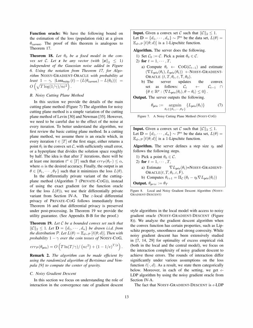
Function oracle: We have the following bound onthe estimation of the loss (population risk) at a givenθcurrent. The proof of this theorem is analogous toTheorem 17.

Theorem 18. Let θ0 be a fixed model in the con-vex set C. Let x be any vector (with ‖x‖2 ≤ 1)independent of the Gaussian noise added in Figure6. Using the notation from Theorem 17, for Algo-rithm NOISY-GRADIENT-ORACLE with probability atleast 1 − γ, |Lossnoisy (t)− (L(θcurrent)− L(θ0))| =

O(√

T log(1/γ)/nε2).

B. Noisy Cutting Plane Method

In this section we provide the details of the maincutting plane method (Figure 7) The algorithm for noisycutting plane method is a simple variation of the cuttingplane method of Levin [30] and Newman [35]. However,we need to be careful due to the effect of the noise atevery iteration. To better understand the algorithm, wefirst review the basic cutting plane method. In a cuttingplane method, we assume there is an oracle which, inevery iteration t ∈ [T ] of the first stage, either returns apoint θt in the convex set C, with sufficiently small error,or a hyperplane that divides the solution space roughlyby half. The idea is that after T iterations, there will beat least one iteration t∗ ∈ [T ] such that errP(θt∗) ≤ α,where α is the desired accuracy. Finally, the output is anθ ∈ θ1, · · · , θT such that it minimizes the loss L(θ).

In the differentially private variant of the cutting-plane method (Algorithm 7 (PRIVATE-COG)), insteadof using the exact gradient (or the function oraclefor the loss L(θ)), we use their differentially privatevariant from Section IV-A. The ε-local differentialprivacy of PRIVATE-COG follows immediately fromTheorem 16 and that differential privacy is preservedunder post-processing. In Theorem 19 we provide theutility guarantee. (See Appendix B-B for the proof.)

Theorem 19. Let C be a bounded convex set such that‖C‖2 ≤ 1. Let D = d1, · · · , dn be drawn i.i.d. fromthe distribution P . Let L(θ) = Ed∼P [`(θ; d)]. Then withprobability 1− γ over the coin tosses of NOISY-COG,

errP(θpriv) = O(T ln(T/γ)/

(nε2)

+ (1− 1/e)T/p).

Remark 2. The algorithm can be made efficient byusing the randomized algorithm of Bertsimas and Vem-pala [9] to compute the center of gravity.

C. Noisy Gradient Descent

In this section we focus on understanding the role ofinteraction in the convergence rate of gradient descent

Input. Given a convex set C such that ‖C‖2 ≤ 1.Let D = d1, · · · , dn ∼ Pn be the data set, L(θ) =Ed∼P [`(θ; d)] is a 1-Lipschitz function.

Algorithm. The server does the following.1) Set C0 := C. Pick a point θ0 ∈ C.2) for t = 1, · · · , T,

a) Compute θt ← COG(Ct−1) and estimate(∇Lpriv(θt), Lpriv(θt)) ←NOISY-GRADIENT-ORACLE (t, T, θt, ε,T, θ0).

b) The server updates the convexset as follows: Ct ← Ct−1 ∩θ ∈ Rp : 〈∇Lpriv(θt), θ − θt〉 ≤ 0 .

Output. The server outputs the following.

θpriv := argminθt∈θ1,··· ,θT

Lpriv(θt) (7)

Figure 7. A Noisy Cutting Plane Method (NOISY-COG)

Input. Given a convex set C such that ‖C‖2 ≤ 1.Let D = d1, · · · , dn ∼ Pn be the data set, L(θ) =Ed∼P [`(θ; d)] is a 1-Lipschitz function.

Algorithm. The server defines a step size ηt andfollows the following steps.

1) Pick a point θ0 ∈ C.2) for t = 1, · · · , T,

a) Estimate ∇Lpriv(θt)=NOISY-GRADIENT-ORACLE(t, T, θt, ε,F).

b) Computes θt+1 = ΠC (θt − ηt∇Lpriv(θt))

Output. θpriv := θT

Figure 8. Local and Noisy Gradient Descent Algorithm (NOISY-GRADIENT-DESCENT)

style algorithms in the local model with access to noisygradient oracle (NOISY-GRADIENT-DESCENT (Figure8)). We analyze the gradient descent algorithm whenthe convex function has certain properties, such as Lip-schitz property, smoothness and strong convexity. Whilenoisy gradient descent has been extensively studiedin [7, 14, 29] for optimality of excess empirical risk(both in the local and the central model), we focus onthe interaction complexity of noisy gradient descent toachieve those errors. The rounds of interaction differsignificantly under various assumptions on the lossfunction `(·, d). As a result, we state them categoricallybelow. Moreover, in each of the setting, we get ε-LDP algorithm by using the noisy gradient oracle fromSection IV-A.

The fact that NOISY-GRADIENT-DESCENT is ε-LDP

13

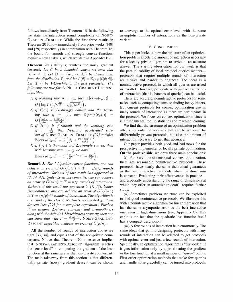
follows immediately from Theorem 16. In the followingwe state the interaction round complexity of NOISY-GRADIENT-DESCENT. While the first three results inTheorem 20 follow immediately from prior works ([40]and [29] respectively) in combination with Theorem 16,the bound for smooth and strongly convex functionsrequire a new analysis, which we state in Appendix B-C.

Theorem 20 (Utility guarantees for noisy gradientdescent). Let C be a bounded convex set such that‖C‖2 ≤ 1. Let D = d1, · · · , dn be drawn i.i.d.from the distribution P , and let L(θ) = Ed∼P [`(θ; d)].Let `(·; ·) be 1-Lipschitz in the first parameter. Thefollowing are true for the NOISY-GRADIENT-DESCENTalgorithm.

1) If learning rate η = 1√t, then E[errP(θpriv)] =

O(

log T(

1/√T +

√p/nε2

)).

2) If `(·; ·) is ∆-strongly convex and the learn-ing rate η = 1

∆t , then E [errP(θpriv)] =

O(

log T∆T + p log(T )

nε2∆

).

3) If `(·; ·) is β-smooth and the learning rateη = 1

∆t , then Nestrov’s accelerated vari-ant of NOISY-GRADIENT-DESCENT [29] satisfiesE [errP(θpriv)] = O

(1T 2 + pT 2 log2 T

nε2β

).

4) If `(·; ·) is β-smooth and ∆-strongly convex, thenwith learning rate η = 1

β we have

E [errP(θpriv)] = O(β2 e−∆T/β + pT

nε2

).

Remark 3. For 1-Lipschitz convex functions, one canachieve an error of O(

√p/n) in T =

√n/p rounds

of interaction. Variants of this result has appeared in[7, 14, 43]. Under ∆-strong convexity, one can achievean error of O(p/n) in T = n/p rounds of interaction.Variants of this result has appeared in [7, 43]. Underβ-smoothness, one can achieve an error of O(

√p/n)

in T = (n/p)1/4 rounds of interaction. The algorithm isa variant of the classic Nestrov’s accelerated gradientdescent (see [29] for a complete exposition.) Further,if we assume ∆-strong convexity and β-smoothnessalong with the default 1-Lipschitzness property, then onecan show that with T = β log(n)

∆ , NOISY-GRADIENT-DESCENT algorithm achieves an error of O(p/n).

All the number of rounds of interaction above aretight [33, 34], and equals that of the non-private coun-terparts. Notice that Theorem 20 in essence impliesthat NOISY-GRADIENT-DESCENT algorithm reachesthe “error level” in computing the gradient of the lossfunction at the same rate as the non-private counterpart.The main takeaway from this section is that differen-tially private (noisy) gradient descent can be shown

to converge to the optimal error level, with the sameasymptotic number of interactions as the non-privatevariant.

V. CONCLUSIONS

This paper looks at how the structure of an optimiza-tion problem affects the amount of interaction necessaryfor a locally-private algorithm to arrive at an accurateanswer. The starting observation for our work is thatthe parallelizability of local protocol queries matters—protocols that require multiple rounds of interactionare slower and harder to engineer. The ideal is anoninteractive protocol, in which all queries are askedin parallel. However, protocols with just a few roundsof interaction (that is, batches of queries) can be useful.

There are accurate, noninteractive protocols for sometasks, such as computing sums or finding heavy hitters.But current protocols for convex optimization use asmany rounds of interaction as there are participants inthe protocol. We focus on convex optimization since itis a fundamental tool in statistics and machine learning.

We find that the structure of an optimization problemaffects not only the accuracy that can be achieved bydifferentially private protocols, but also the amount ofinteraction necessary to get that accuracy.

Our paper provides both good and bad news for theprospective implementer of locally private optimization.On the positive side, we draw three main conclusions:

(i) For very low-dimensional convex optimization,there are reasonable noninteractive protocols. Theseprotocols have nearly the same theoretical guaranteesas the best interactive protocols when the dimensionis constant. Evaluating their effectiveness in practice—and especially understanding the range of dimensions atwhich they offer an attractive tradeoff—requires furtherstudy.

(ii) Sometimes problem structure can be exploitedto find good noninteractive protocols. We illustrate thiswith a noninteractive algorithm for linear regression thathas the same asymptotic error as the best interactiveone, even in high dimensions (see, Appendix C). Thisexploits the fact that the quadratic loss function itselfhas a compact description.

(iii) A few rounds of interaction help enormously. Thesame ideas that go into designing protocols with manyrounds of interaction can be adapted to get protocolswith optimal error and just a few rounds of interaction.Specifically, an optimization algorithm is “first-order” ifit gets information only by approximating the gradientor the loss function at a small number of “query” points.First-order optimization methods that make few queriesand handle noise gracefully can be turned into protocols

14

that use few rounds of interaction. We demonstrate thisfor gradient descent and the cutting plane method.

The best choice of algorithm depends on the tradeoffbetween various aspects of the problem structure (di-mension, smoothness, strong convexity); see Figure 2.Interestingly, the smoothness of a problem does not af-fect the error achievable by the best differentially privatealgorithm, but it can drastically reduce interaction.

Unfortunately, for general convex optimization (thatis, without assuming both smoothness and strong con-vexity), our protocols still require a number of roundsof interaction that grows polynomially with the problemdimension.On the negative side, we show:

(iv) Known algorithmic design techniques forlocal private learning cannot provide noninterac-tive protocols—or even ones with few rounds ofinteraction—for general convex optimization in highdimensions. Specifically, any first-order optimizationalgorithm must either have “many” batches of queries,or make exponentially-many queries (in the dimensionp) in order to have nontrivial accuracy. Here “many”depends on the desired accuracy—the lower bound isabout log(1/α) for desired error α. That means thatevery nonadaptive first-order algorithm (one that asksall its queries in one batch) must make exponentiallymany queries to be useful. Consequently, very differenttechniques are needed for noninteractive, general pur-pose local optimization.

Both our positive and negative results highlight therole of several key structural properties: (a) The di-mension p, that is the number of real parameters inthe vectors θ over which we aim to minimize a lossfunction. (b) The variability of the loss function weaim to minimize; measures of variability include the“Lipschitz constant”—an upper bound on the amountthat any one individual can change the gradient of theloss function—and the smoothness, which is an upperbound on the rate at which the gradient changes as θvaries. For example, the loss function for support vectormachines has low Lipschitiz constant but is not smooth(the gradient changes abruptly). (c) The strong convexityof the loss function. A strongly convex function isbounded below by a quadratic function at every pointand, in particular, has a well-defined minimum. (d) Theshape and size of the constraint set C in which θ resides.We focus here on the role of the diameter of C, thoughother work on (central) differential privacy suggeststhat properties (the Gaussian width, and the number ofexptreme points) [43] also play a role.

Perhaps the simplest conclusion is that these struc-tural properties are important, and a prospective imple-

menter’s first task is to extract as much structure aspossible from the specific problem and include theseextra properties explicitly in the problem formulation.

The importance and difficulty of evaluation. Thispaper focuses on the analytical evaluation of severalalgorithms and advances some basic design principles.One of the lessons of our work is that there is currentlyno single all-purpose algorithm for local private learn-ing, and so the choice of the best algorithm is likely todepend on the problem and the data at hand. That high-lights the need for further algorithmic research—whatnew techniques can we bring to bear? can we bypassthe lower bounds in this paper by using algorithms thataccess the loss function differently?—as well as careful,application-specific empirical evaluation. We hope thisstudy informs such efforts, both by suggesting specificalgorithms and highlighting structural properties thatplay an important role.

ACKNOWLEDGMENTS

We are grateful to Vitaly Feldman, Ilya Mironov, andKunal Talwar for helpful conversations about this prob-lem, as well as to David Evans and several anonymousreferees for their detailed and constructive feedback onthe submitted version. We would like to thank PrateekJain especially for some of the ideas in the convergenceproof of gradient descent with smooth and stronglyconvex functions. A.S. and J.U. are supported by NSFaward IIS-1447700, a Google Faculty Award and aSloan Foundation research award.

REFERENCES

[1] Privacy by the numbers: A new approach to safeguard-ing data. Scientific American, 2012.

[2] Apple tries to peek at user habits without violatingprivacy. The Wall Street Journal, 2016.

[3] A. Agarwal, M. J. Wainwright, P. L. Bartlett, and P. K.Ravikumar. Information-theoretic lower bounds on theoracle complexity of convex optimization. In NIPS,pages 1–9, 2009.

[4] S. Agrawal, J. R. Haritsa, and B. A. Prakash. Frapp: aframework for high-accuracy privacy-preserving mining.Data Mining and Knowledge Discovery, 18(1):101–139,2009.

[5] K. Ball. An elementary introduction to modern convexgeometry. Flavors of geometry, 31:1–58, 1997.

[6] R. Bassily and A. Smith. Local, private, efficientprotocols for succinct histograms. In STOC, pages 127–135. ACM, 2015.

[7] R. Bassily, A. Smith, and A. Thakurta. Private empiricalrisk minimization: Efficient algorithms and tight errorbounds. In FOCS, pages 464–473. IEEE, 2014.

[8] A. Beimel, K. Nissim, and E. Omri. Distributed privatedata analysis: Simultaneously solving how and what. InCRYPTO, pages 451–468. Springer, 2008.

15

[9] D. Bertsimas and S. Vempala. Solving convex programsby random walks. JACM, 51(4):540–556, 2004.

[10] S. Bubeck. Convex optimization: Algorithms and com-plexity. Foundations and Trends in Machine Learning,8(3-4):231–357, 2015.

[11] P. Burgisser and F. Cucker. Condition: The geometry ofnumerical algorithms, volume 349. Springer Science &Business Media, 2013.

[12] T.-H. H. Chan, E. Shi, and D. Song. Private andcontinual release of statistics. ACM Trans. Inf. Syst.Secur., 14(3):26, 2011.

[13] K. Chaudhuri, C. Monteleoni, and A. D. Sarwate. Dif-ferentially private empirical risk minimization. JMLR,12(Mar):1069–1109, 2011.

[14] J. C. Duchi, M. I. Jordan, and M. J. Wainwright. Localprivacy and statistical minimax rates. In FOCS, pages429–438. IEEE, 2013.

[15] C. Dwork and A. Roth. The algorithmic foundationsof differential privacy. Foundations and Trends inTheoretical Computer Science, 9(3-4):211–407, 2014.

[16] C. Dwork, K. Kenthapadi, F. McSherry, I. Mironov, andM. Naor. Our data, ourselves: Privacy via distributednoise generation. In EUROCRYPT, 2006.

[17] C. Dwork, F. McSherry, K. Nissim, and A. Smith.Calibrating noise to sensitivity in private data analysis.In TCC, pages 265–284. Springer, 2006.

[18] C. Dwork, M. Naor, T. Pitassi, and G. N. Rothblum.Differential privacy under continual observation. InSTOC, pages 715-724, ACM, 2010.

[19] U. Erlingsson, V. Pihur, and A. Korolova. Rappor:Randomized aggregatable privacy-preserving ordinal re-sponse. In CCS, pages 1054–1067. ACM, 2014.

[20] A. Evfimievski, J. Gehrke, and R. Srikant. Limitingprivacy breaches in privacy preserving data mining. InPODS, pages 211–222. ACM, 2003.

[21] V. Feldman, C. Guzman, and S. Vempala. Statisticalquery algorithms for stochastic convex optimization.arXiv:1512.09170, 2015.

[22] M. Hay, V. Rastogi, G. Miklau, and D. Suciu. Boost-ing the Accuracy of Differentially Private HistogramsThrough Consistency. PVLDB, 3(1):1021–1032, 2010.

[23] J. Hsu, S. Khanna, and A. Roth. Distributed privateheavy hitters. In ICALP, pages 461–472. Springer, 2012.

[24] P. Jain, P. Kothari, and A. Thakurta. Differentiallyprivate online learning. In COLT, pages 24–1, 2012.

[25] S. P. Kasiviswanathan and A. Smith. On the’semantics’of differential privacy: A bayesian formulation. Journalof Privacy and Confidentiality, 6(1):1, 2014.

[26] S. P. Kasiviswanathan, H. K. Lee, K. Nissim,S. Raskhodnikova, and A. Smith. What can we learnprivately? SIAM Journal on Computing, 40(3):793–826,2011.

[27] M. Kearns. Efficient noise-tolerant learning from statis-tical queries. JACM, 45(6):983–1006, 1998.

[28] D. Kifer, A. Smith, and A. Thakurta. Private convexempirical risk minimization and high-dimensional re-gression. JMLR, 1:41, 2012.

[29] G. Lan. An optimal method for stochastic compositeoptimization. Mathematical Programming, 133(1-2):365–397, 2012.

[30] A. Y. Levin. On an algorithm for the minimization

of convex functions. In Soviet Mathematics Doklady,volume 160, pages 1244–1247, 1965.

[31] F. J. MacWilliams and N. J. A. Sloane. The theory oferror correcting codes. Elsevier, 1977.

[32] N. Mishra and M. Sandler. Privacy via pseudorandomsketches. In SIGMOD, pages 143–152. ACM, 2006.

[33] A. Nemirovski, D.-B. Yudin, and E.-R. Dawson. Prob-lem complexity and method efficiency in optimization.1982.

[34] Y. Nesterov. Introductory lectures on convex optimiza-tion: A basic course, volume 87. Springer Science &Business Media, 2013.

[35] D. J. Newman. Location of the maximum on unimodalsurfaces. JACM, 12(3):395–398, 1965.

[36] Z. Qin, Y. Yang, T. Yu, I. Khalil, X. Xiao, and K. Ren.Heavy hitter estimation over set-valued data with localdifferential privacy. In CCS, pages 192–203. ACM,2016.

[37] M. Raginsky and A. Rakhlin. Information-based com-plexity, feedback and dynamics in convex program-ming. IEEE Transactions on Information Theory, 57(10):7036–7056, 2011.

[38] M. Rudelson and R. Vershynin. The smallest singularvalue of a random rectangular matrix. Communicationson Pure and Applied Mathematics, pages 1707 – 1739,2009.

[39] S. Shalev-Shwartz, O. Shamir, N. Srebro, and K. Srid-haran. Stochastic Convex Optimization. In COLT, 2009.

[40] O. Shamir and T. Zhang. Stochastic gradient descentfor non-smooth optimization: Convergence results andoptimal averaging schemes. In ICML (1), pages 71–79,2013.

[41] A. Smith and A. Thakurta. Differentially private modelselection via stability arguments and the robustness ofthe lasso. J Mach Learn Res Proc Track, 30:819–850,2013.

[42] S. Song, K. Chaudhuri, and A. D. Sarwate. Stochasticgradient descent with differentially private updates. InGlobalSIP, pages 245–248. IEEE, 2013.

[43] K. Talwar, A. Thakurta, and L. Zhang. Nearly optimalprivate lasso. In NIPS, 2015.

[44] A. G. Thakurta and A. Smith. (nearly) optimal algo-rithms for private online learning in full-information andbandit settings. In NIPS, pages 2733–2741, 2013.

[45] R. Vershynin. Introduction to the non-asymptotic anal-ysis of random matrices. arXiv:1011.3027, 2010.

[46] S. L. Warner. Randomized response: A survey techniquefor eliminating evasive answer bias. Journal of theAmerican Statistical Association, 60(309):63–69, 1965.

[47] O. Williams and F. McSherry. Probabilistic inferenceand differential privacy. In NIPS, pages 2451–2459,2010.

[48] Y. Yang and A. Barron. Information-theoretic deter-mination of minimax rates of convergence. Annals ofStatistics, pages 1564–1599, 1999.

APPENDIX A.LOCAL RANDOMIZER FOR ε-LDP

Randomizer of Duchi et al. [14]. On input x ∈ Rp, therandomizer Rε(x) does the following. It first sets x =

16

bx/‖x‖2, where b ∈ −1, 1 Bernoulli random variableBer(1/2 + ‖x‖/2). We then sample T ∼ Ber(eε/(eε +1)) and outputs Rε(x), where

Rε(x) :=

Uni(u ∈ Rp : 〈u, x〉 > 0) if T = 1

Uni(u ∈ Rp : 〈u, x〉 ≤ 0) if T = 0.

Let y be any unit vector independent of the inputto the randomizer x. An alternate way to see therandomizer Rε(x) is that the output of Rε(·) is suchthat 〈y,Rε(x)〉 = 〈y, cε,dBu,xu〉 for cε,p = O(

√p/ε)

and Bu,x is ±1 random variable chosen such thatE[Rε(x)] = x. In the following we prove Theorem17, the utility guarantee we desire from our NOISY-GRADIENT-ORACLE.

Proof of Theorem 17: Duchi et al. [14, SectionV.C] proved that Rε(x) is an unbiased estimator, i.e.,E [Gradnoisy (t)] = ∇L(θcurrent); therefore, the first partfollows. In order to show the second and the third partof Theorem 17 , we show that the randomizer has sub-gaussian tail (see Definition 21 and Theorem 22 below).

Definition 21. A real-valued random variable X is sub-gaussian if it has the property that there is some c > 0such that for every t ∈ R one has E[etX ] ≤ ec

2t2/2.Moreover, Var(X) = c2.

Theorem 22. Given a vector x ∈ Rp, the randomizer ofDuchi et al. [14] defined above is a subgaussian randomvector with variance O(p/ε2).

Proof: In the following, we use the notationMX(t) = E[etX ] to denote the moment generat-ing function of the random variable X . Let Av,x =〈v, cε,dBu,xu〉. In order to prove that the randomizer ofDuchi et al. [14] outputs a subgaussian random vector,it suffices to prove that Av,x is subgaussian.

MAv,x(t) = E[etAv,x ] = E[etcε,p〈v,u〉 + e−tcε,p〈v,u〉]

= M〈v,u〉(cε,pt) +M〈v,u〉(−cε,pt)= M〈v,u〉(cε,pt) ≤ 2ec

2ε,pt

2/2 = 2et2p/ε2 .

Using Definition 21 completes the proof.For the second part, notice that, by definition, the

set St (the current batch in Algorithm 6) has Θ(n/k)entries and every user in the set St randomizes itsoutput independently of the others. This observation,along with with Theorem 22, allows us to bound thevariance of the estimator Gradnoisy (t) in (8) below. Herewe use the fact that ‖∇`(θ; d)‖2 ≤ 1 for for all θ ∈ Cand d ∈ D (where C is the convex set over which theoptimization is performed, and D is the domain of the

data entries).

E[‖Gradnoisy (t)−∇L(θcurrent)‖22

]= (T/n)Var(Rε(x))

= O(Tp/nε2

). (8)

To prove the third part of Theorem 17, weprovide a tail bound on the the inner product〈Gradnoisy (t), y〉 for any vector y s.t. ‖y‖2 ≤ 1and is independent of Rε(x). Now, by standard tailbound for sub-gaussian distribution [45], we have,Pr[|〈Rε(x), y〉| = O

(√T log(1/γ)/ε2n

)]≥ 1 −

γ.This completes the proof of Theorem 17.

APPENDIX B.MISSING PROOFS

A. Proof of Claim 4

Proof: In the net-based argument, one would firstconstruct an α/2-net over the convex set of size m andthen find the minimum over each of these net points.To make it local-differentially private, we need to usethe randomizer of Duchi et al. [14]. This would incur a

total population error, O(√

m logm log(1/γ)ε2n + α

2

)with

probability 1− γ. In a p-dimensional space [0, 1]p, weneed to have m = O((2/α)p) net points. Setting thisvalue of m, we get the population error

O

(√(2

α

)pp log(2/α) log(1/γ)

ε2n+α

2

). (9)

To minimize equation (9), we need αp+2ε2n =2p+1p log(2/α) log(1/γ). In other words, the popu-

lation error is at most O

((p log(1/γ)

ε2n

)1/(p+2))

In

other words, equation (1) implies that one need n =

Ω(

p4p

ε2αp+2

)to get errD(θpriv) ≤ α.

B. Proof of Theorem 19

Proof: We first state the following claim. Theclaims allows us to work with an easy to handle functionM(·).

Claim 23. Let θ∗ = argminθ∈C L(θ), and let M(θ) :=L(θ)−L(θ0), where θ0 is as in the first step of Figure 7.Then the following holds : (i) θ∗ = argminθ∈CM(θ),(ii) ∀θ ∈ C, L(θ)− L(θ∗) = M(θ)−M(θ∗).

Proof: The first part of the claim follows fromthe fact that L(θ0) is a constant, and subtracting aconstant from the objective function does not change theargument of the optimum value. The second part fol-lows from the following straightforward computation:M(θ)−M(θ∗) = L(θ)− L(θ0)− L(θ∗) + L(θ0).Thiscompletes the proof of Claim 23.

17

We will use the following result about non-privatecutting plane method.

Lemma 24. [10, Theorem 2.1] Let C and p be asdefined in Theorem 19. Let θ∗ = argminθ∈C L(θ) andCt be as defined in Figure 7 for iteration t ∈ [T ]. LetE be the event that θ∗ ∈ Ct for all iterations t ≤ T .Conditioned on the event E, there exists an iterationτ ∈ [T ], such that M(θτ ) satisfies the following bound.

M(θτ )−M(θ∗) ≤ 2 (1− 1/e)T/p

.

We now analyze the algorithm presented in Figure 7.Our first lemma states the condition when the optimalpoint is not excluded by NOISY-COG.

Lemma 25. Let θ∗ = argminθ∈C L(θ). Let gt =∇Lpriv(θt) − ∇L(θt) for 0 < t ≤ T . If for all τ ≤t ∈ [T ], 〈gt, θt − θ∗〉 ≥ −α and M(θt)−M(θ∗) ≥ α,then θ∗ ∈ Cτ , where Cτ is the convex set included afterτ rounds.

Proof: Since the function M(·) is convex, we haveM(θ) ≥M(θt) + 〈∇M(θt), θ − θt〉 for all θ ∈ C. Thisimplies that 〈∇M(θt), θt − θ〉 ≥M(θt)−M(θ)

Let α be a parameter that we will fix later.Now, if M(θt) − M(θ∗) ≥ α, then we have〈∇M(θt), θt − θ∗〉 ≥ M(θt) − M(θ∗) ≥ α. Thisfurther implies that 〈∇M(θt), θ

∗ − θt〉 ≤ −α. Fromthe description of NOISY-COG, we exclude all θ ∈ Csuch that 〈∇M(θt), θ − θt〉 ≥ 〈gt, θ − θt〉. Combiningthese observations completes the proof of Lemma 25.

Lemma 26. Let θ∗ = argminθ∈CM(θ). Then withprobability 1−γ over the coin tosses of PRIVATE-COG,there exists a t ∈ [T ] such that

M(θt)−M(θ∗) = O(√

T log(T/γ)/nε2 + (1− 1/e)Tp

).

Proof: From Theorem 17, for all t ∈ [T ] wehave with probability at least 1 − γ, |〈gt, θt − θ∗〉| =

O(√

T log(1/γ)/nε2), where gt = ∇Lpriv(θt) −

∇L(θt) for 0 < t ≤ T . If we pick α =

O(√

T log(T/γ)/nε2), then taking union bound over

all the T rounds, Pr [∀t ∈ [T ], 〈gt, θ∗ − θt〉 ≤ −α] ≤ γ.Lemma 26 now follows from Lemma 24 and 25.

Lemma 26 and Theorem 18 gives Theorem 19.

C. Analysis for 1-Lipschitz, β-smooth and ∆-stronglyConvex Functions

In the following we provide the analysis of part (4)from Theorem 20.

Proof of Theorem 20 (4): Let θ∗ = minθ∈C

L(θ),

Dt = θt−θ∗ and zt+1 = θt−η(Rε(∇L(θt))). Let gt =

(∇Lpriv(θt)−∇L(θt)) be the error in the estimationin Algorithm PRIVATE-GRADIENT-ORACLE (Figure 6)for t ∈ [T ]. First, by the Pythogorean theorem, we have,

‖Dt+1 −Dt‖22 = ‖Dt‖22 + ‖Dt+1‖22 − 2〈Dt, Dt+1〉.(10)

Using the β-smoothness and ∆-strong convexity, wehave the following:

L(θt+1)− L(θ∗) = L(θt+1)− L(θt) + L(θt)− L(θ∗)

≤ 〈∇L(θt), Dt+1〉+β

2‖θt+1 − θt‖22 −

∆

2‖Dt‖22

= 〈1η

(θt − zt+1)− gt, θt+1 − θ∗〉

+β

2‖θt+1 − θt‖22 −

∆

2‖θt − θ∗‖22

= 〈1η

(θt + θt+1 − θt+1 − zt+1)− gt, θt+1 − θ∗〉

+β

2‖θt+1 − θt‖22 −

∆

2‖θt − θ∗‖22

≤ 1

η〈θt − θ∗, θt+1 − θ∗〉 − 〈gt, θt+1 − θ∗〉

− 1

η‖Dt+1‖22 +

β

2‖θt+1 − θt‖22 −

∆

2‖Dt‖22.

(11)

Let wt+1 = θt − η∇L(θt). Now,

E[〈gt, θt+1 − θ∗〉] = E[〈gt, θt+1 −ΠC(wt+1)〉]+ E[〈gt,ΠC(wt+1)− θ∗〉]

= E[〈gt, θt+1 −ΠC(wt+1)〉]≤ E[‖gt‖2‖θt+1 −ΠC(wt+1)‖2]

≤ E[‖gt‖2‖zt+1 − wt+1)‖2]. (12)

Substituting equation (10) and equation (12) in equa-tion (11), and then using the bound on gt from Theorem17, for all 1 ≤ t ≤ T , we get

2E[L(θt+1, d)− L(θ∗, d)]

≤(

1

η−∆

)E[‖Dt‖22]− 1

ηE[‖Dt+1‖22]

+

(β − 1

η

)E[‖Dt −Dt+1‖22] +O

(Tp/

(nε2)).

≤(

1

η−∆

)E[‖Dt‖22]− 1

ηE[‖Dt+1‖22] +O

(Tp/

(nε2)).

(13)

Since E[L(θt+1)−L(θ∗)] ≥ 0, equation (13) impliesthat

E[‖Dt+1‖22] ≤ (1− η∆)E[‖Dt‖22] + η ·O(Tp/

(nε2)).

(14)

18

Let ‖θ0 − θ∗‖2 ≤ 1, then using the above equations,we get

E[‖DT ‖22] ≤ e−η∆T + η

(1− e−η∆T

1− e−η∆

)·O(Tpσ2

nε2

)≤ e−η∆T + η ·O

(Tp/

(nε2)). (15)

Using the fact that the function is β-smooth, i.e.,E[errD(θpriv)] ≤ β

2E[‖DT ‖22] and setting η = 1β , and

we have Theorem 20.

APPENDIX C.CASE STUDY: LINEAR REGRESSION

In this section we concentrate on a specific problemof linear regression in the LDP model. We give asimple non-interactive algorithm that outputs an esti-mate (Theorem 27). We show that the error guaranteeachieved by this algorithm is the best one can hopefor by showing a matching lower bound (Theorem 31).Our algorithm satisfies a slightly weaker variant ofthe privacy definition in Definition 1, called (ε, δ)-approxmiate differential privacy [16], where the def-inition of closeness in Definition 1 is modified toPr[Q(d) ∈ E] ≤ eε Pr[Q(d′) ∈ E] + δ. Considerδ ≈ 1/nω(1), where n is the number of data samples.

A. Local-Differentially Private Linear Regression

Let X1, · · · ,Xn ∈ Rp be row vectors and y ∈ Rnbe a column vector, where di := (Xi, yi) ∈ Rp+1 is thedata of the user i and D := (d1, · · · , dn) be the dataset.We present this section in the terms of empirical risk.Using standard results [39], this bound can be convertedto population risk with no difference in the asymptoticbound. For linear regression, we know that the lossfunction has the following closed form expression.

`(θ; (Xi, yi)) := (yi − 〈Xi, θ〉)2, (16)

L(θ;D) :=1

2n

n∑i=1

`(θ; di) =1

2n‖y− Xθ‖22. (17)

and the minimizer has the form θ∗ :=argminθ∈C

12n‖y − Xθ‖22. We show that it is possible

to non-interactively compute a θpriv in (ε, δ)-local-differentially private manner. More precisely, we showthe following.

Theorem 27. Let C ⊆ Rp be a bounded convex set(‖C‖2 ≤ 1) over which the linear regression problem isdefined. There is an efficient non-interactive algorithmthat solves linear regression problem, stated in equa-tion (17), while preserving (ε, δ)-local differential pri-vacy such that with probability at least 99/100 over the

coin tosses of the algorithm,

errD(θpriv) = O(√

p log(1/δ)/ (nε2)).

Proof: Note that ‖y − Xθ‖22 = ‖y‖22 − 2〈Xθ, y〉 +〈Xθ,Xθ〉. Since the first term does not depend on θ,this implies that

argminθ∈C

1

2n‖y− Xθ‖22 = argmin

θ∈C

1

2n〈Xθ,Xθ〉 − 2〈Xθ, y〉.

We maintain the following two quantities:

1) Noisy covariance: Z := XTX + B, where B ∼N (0, 2n log(1/δ)/ε2)p×p; and

2) Noisy terms, z := (∑

yiXi) + b, where b ∼N (0, 2n log(1/δ)/ε2)1×p.

This can be achieved in the local model as follows:every user computes Zi := XT

i Xi + Bi, where Bi ∼N (0, 2 log(1/δ)/ε2)p×p and zi := yiXi + bi, wherebi ∼ N (0, 2 log(1/δ)/ε2)1×p. The user then sends(Zi, zi) to the server. The server can now computeZ =

∑i Zi and z =

∑zi. This results in the same

noisy covariance and noisy term as above becauseXTX =

∑ni=1 XT

i Xi and the noise matrix B1, · · · ,Bn

and the noise vector b1, · · · ,bn are independent.Now let us define

Lpriv(θ;D) :=1

2n

(‖y‖22 − 2

∑〈yiXT

i + b, θ〉)

+1

2n

(θT(XTX + B)θ

)and let the minimizer of Lpriv(θ;D) be θpriv.

From now on, we write L(·) instead of L(·;D)and Lpriv(·) instead of Lpriv(·;D). We can decomposeL(θpriv)− L(θ∗) as following:

L(θpriv)− L(θ∗) = L(θpriv)− Lpriv(θpriv) + Lpriv(θpriv)

− Lpriv(θ∗) + Lpriv(θ

∗)− L(θ∗)

≤ L(θpriv)− Lpriv(θpriv) + Lpriv(θ∗)− L(θ∗)

≤2‖b‖2‖θpriv − θ∗‖2 + θTprivBθpriv − (θ∗)TBθ∗

2n.

(18)

The first inequality follows from the fact thatLpriv(θpriv) − Lpriv(θ

∗) ≤ 0 (since θ∗ is the minimizer)and the second inequality follows from the fact that〈·, ·〉 ≤ ‖ · ‖2‖ · ‖2. Let β = θpriv − θ∗. We can furtherdecompose θTprivBθpriv as follows.

θTprivBθpriv = (θ∗)TBθ∗ + βTBθ∗ + (θ∗)TBβ + βTBβ(19)

19

Now using equation (19) in equation (18), the boundon the singular values of Gaussian matrices [38] andthat ‖C‖2 ≤ 1, we get

L(θpriv)− L(θ∗) ≤1

2n(2‖b‖2‖θpriv − θ∗‖2)

+1

2n

(λmax(B)‖θpriv − θ∗‖22

)+

1

2n(2λmax(B)‖θpriv − θ∗‖2‖C‖2)

= O(√

p log(1/δ)/ (nε2)).

This completes the proof ot Theorem 27.

B. Lower Bound on Linear Regression

In this section we prove that the error bound achievedin Theorem 27 is optimal.

Minimax rates. We use the framework of minimaxrates introduced by Duchi et al. [14] to prove the lowerbound. Let S ⊂ [0, 1]|D| denote the simplex with |D|corners, each representing one of the possible datasets.Let P ∈ S be a probability distribution over the datasetsD. User i data di is assumed to be drawn i.i.d. using thedistribution P. For every user i, let Ri(·) be the localrandomizer of the user i which is used to generate thereport Zi = Ri(di) ∈ Z . Each of these randomizersare assumed to use independent random bits. Let Algbe an algorithm that is used to estimate the distributionP based on Z1, · · · , Zn. The minimax rate is definedas follows:

MinMax := minAlg

maxP

E[‖Alg(Z1, · · · , Zn)−P‖∞].

Now that we have described our framework to provethe lower bound, we sketch our proof. Our proof usesidea in Bassily and Smith [6]. In order to use their idea,we need to first introduce the notion of an γ-degradingchannel. For any γ ∈ [0, 1], an γ-degrading channelW γ : D → D is a randomized mapping that is definedas follows: for every d ∈ D,

W γ(d) :=

d with probability γ0 otherwise

(20)

Let MinMaxγ be the minimax error resulting from thescenario where each user i ∈ [n] with data di ∈ Dfirst applies di to an independent copy W γ of an γ-degrading channel, and then apply the output to its (ε, δ)local-differentially private algorithm Ri that outputs Zi.That is, MinMaxγ is the minimax error when Ri(·) isreplaced by Ri(W γ

i (·)) for all i ∈ [n]. We first provethe following claim.

Claim 28. If MinMax ≥ 0.01, then MinMaxγ ≥ 0.01γ

Proof: Let W γ = γD. Then Ed∼Wγ [`(θ; d)] =γEd∼D[`(θ; d)] ≥ γ

100 . This completes the proofof Claim 28.

We now construct a hard instance of input to any LDPalgorithm. Let H be the p-dimensional hypercube that isjust contained inside Bp. Consider a codeword which isthe subset of the coordinates of H and has distance p/8.Using Gilbert-Varshamov bound [31], we know that thesize of the codeword is N ≥ 2p/8. We pick N distri-butions D1, · · · ,DN . Each of these distributions are apoint distribution such that y − 〈X, θ〉 = 1 ⇔ θ∗i = X.Our result follows from the following claims:

Claim 29. Let θpriv be the output of an algorithm thatsolves the linear regression problem. Then the mutualinformation between θpriv and the distribution of thedata points is I(θpriv;D) ≤ nε2γ2, where γ is theparameter for the degrading channel.

Proof: Using the chain rule of mutual informationand Duchi et al. [14], we have the following:

I(θpriv; d) ≤ I(Z1, · · · , Zn; d) ≤ 4(eε − 1)2n ≤ 16ε2n

The claim now follows from Bassily and Smith [6].

Claim 30. For any Di, let Si1/100 :=θ ∈ Bp : L(θ;D) ≤ 1/100

, where D ∼ Di,

then ∀i, j, i 6= j, Si1/100 ∩ Sj1/100 = 0.

Proof: Let i and j be adjacent node on the hyper-cube H. Let Q be the intersection (of the extension)of the sets Si1/100 and Si1/100. Let C be the center ofthe ball Bp. First note that the boundary of Si1/100 andSj1/100 are hyperplane whose normal intersects at C. Letζ be the angle made by the normal of the hyperplanecorresponding to Si1/100 and the line passing throughC and Q. First of all, sin ζ =

√1/32, and cos ζ =√

31/32.By symmetry, the line CQ cuts the line between node-

i and node-j into half. Therefore, the length of CQ is9

10√

31/32≥ 1. This implies that Q lies outside Bp.

We now complete the proof of the main result.

Theorem 31. Any ε-local differential private algorithmfor linear regression incurs an error Ω(

√p/nε2).

Proof: By Fano’s inequality [48] and Claim 29,

Pr[θipriv /∈ Si1/100

]≥ 1− I(θpriv;D)

logN≥ 1− 8cnε2γ2

p.

Then Claim 30 gives us that MinMax ≥10−2

(1− 8cnε2γ2/p

). For γ = O(

√pnε2 ), we get

MinMax ≥ 1/100. By Claim 28, we have the overallerror Ω

(√pnε2

).

20