Is High Public Debt Always Harmful to Economic Growth

HAL Id: halshs-00700471https://halshs.archives-ouvertes.fr/halshs-00700471

Preprint submitted on 23 May 2012

HAL is a multi-disciplinary open accessarchive for the deposit and dissemination of sci-entific research documents, whether they are pub-lished or not. The documents may come fromteaching and research institutions in France orabroad, or from public or private research centers.

L’archive ouverte pluridisciplinaire HAL, estdestinée au dépôt et à la diffusion de documentsscientifiques de niveau recherche, publiés ou non,émanant des établissements d’enseignement et derecherche français ou étrangers, des laboratoirespublics ou privés.

Is High Public Debt Always Harmful to EconomicGrowth? Reinhart and Rogoff and some complex

nonlinearitiesAlexandru Minea, Antoine Parent

To cite this version:Alexandru Minea, Antoine Parent. Is High Public Debt Always Harmful to Economic Growth? Rein-hart and Rogoff and some complex nonlinearities. 2012. �halshs-00700471�

https://halshs.archives-ouvertes.fr/halshs-00700471

https://hal.archives-ouvertes.fr

CERDI, Etudes et Documents, E 2012.18

1

C E N T R E D ' E T U D E S

E T D E R E C H E R C H E S

S U R L E D E V E L O P P E M E N T

I N T E R N A T I O N A L

Document de travail de la série

Etudes et Documents

E 2012.18

Is High Public Debt Always Harmful to Economic Growth?

Reinhart and Rogoff and some complex nonlinearities

Alexandru Minea§ and Antoine Parent

#

February 2012

CERDI

65 BD. F. MITTERRAND

63000 CLERMONT FERRAND - FRANCE

TEL. 04 73 17 74 00

FAX 04 73 17 74 28

www.cerdi.org

§ Corresponding Author: CERDI (University of Auvergne), 65 Boulevard François Mitterrand, BP 320, 63009

Clermont-Ferrand Cedex 1, France. Email: [email protected]. # BETA-REGLES (University of Nancy 2), 13 Place Carnot, CO 26, 54035 Nancy Cedex. Email:

[email protected].


2

La série des Etudes et Documents du CERDI est consultable sur le site :

http://www.cerdi.org/ed

Directeur de la publication : Patrick Plane

Directeur de la rédaction : Catherine Araujo Bonjean

Responsable d’édition : Annie Cohade

ISSN : 2114-7957

Avertissement :

Les commentaires et analyses développés n’engagent que leurs auteurs qui restent seuls

responsables des erreurs et insuffisances.


3

Is High Public Debt Always Harmful to Economic Growth?

Reinhart and Rogoff and some complex nonlinearities

Alexandru Minea§ and Antoine Parent

#

February 2012

Abstract: In their already-famous 2010 article “Growth-in-a-Time-of-Debt”

(AER-100(2)-pp.-573-78), Carmen Reinhart and Kenneth Rogoff show that

average post-WW2 economic growth is dramatically declining in advanced

economies, once the debt-to-GDP ratio is above a 90% threshold. We

explore the relevance of this exogenous threshold using up-to-date

econometric techniques, and reveal an endogenously-estimated threshold

around a debt-to-GDP ratio of 115%, above which the negative debt-growth

link changes sign. Consequently, additional evidence is needed before

suggesting policy recommendations regarding growth effects of fiscal policy

in such high debt regimes, which may be subject to complex nonlinearities.

Keywords: public debt, economic growth, nonlinear effects, cliometrics.

JEL Codes: H63, E62, N10

§ Corresponding Author: CERDI (University of Auvergne), 65 Boulevard François Mitterrand, BP 320, 63009

Clermont-Ferrand Cedex 1, France. Email: [email protected]. # BETA-REGLES (University of Nancy 2), 13 Place Carnot, CO 26, 54035 Nancy Cedex. Email:

[email protected].


4

I. Introduction

In their already-famous article “Growth in a Time of Debt”, published by The American

Economic Review in 2010 (AER 100(2), pp. 573-78), Carmen Reinhart and Kenneth Rogoff

analyze the relation between economic growth and public debt.1 Drawing upon a new public

debt database, Reinhart & Rogoff (2010, hereafter RR) exhibit the presence of debt-to-GDP

ratios that they assess in terms of threshold. Regarding advanced economies, RR show that

post-WW2 economic growth is dramatically declining on average once the public debt-to-

GDP ratio is above the 90% threshold. Policy recommendations by official institutions,

including the OECD, the EU Commission or the French Report on Public Finance (April

2010), seem to have adopted this threshold as an ultimate guide for policy making, by taking

for granted the “Reinhart and Rogoff’s debt intolerance ratio” and transforming it, rather

mechanically, into a “natural” target to shift public spending.

The goal of the present manuscript is to contribute to the current strand of literature on

public debt and economic growth,2 by exploring the relevance of the 90% threshold

emphasized by RR. Using up-to-date econometric techniques, which allow dealing properly

with complex nonlinearities on panel data, we find the existence of an endogenously-

estimated threshold, at roughly 115%, in the public debt to economic growth relation. Below

this threshold, a debt increase damages growth; however, this negative effect is declining as

public debt is increasing. Above this threshold, the link between public debt and economic

growth changes sign.

In light of these estimations, we reproduce the stylized facts emphasized by RR. On

the one hand, we show that, similarly to RR, average economic growth is lower for countries

with debt levels between 90 and 115%, compared to countries with debt levels between 60

and 90%. On the other hand, we show that average economic growth is higher for countries

with public debt above 115%, compared to countries with debt levels between 90 and 115%,

and more importantly, that average economic growth is not statistically different for the

former group compared to countries with debt levels between 60 and 90%. Although one

should reasonably refrain from concluding that governments should adopt loose fiscal

policies, leading to high public debt levels, to foster economic growth, this latter result

provides a new perspective on the “debt intolerance ratio” emphasized by RR. Indeed, an

1 To better focus our analysis, we leave for further investigation the issue of economic growth and inflation,

equally discussed by Reinhart & Rogoff (2010). 2 For a recent survey on this literature, see Parent (2012).


5

increasing public debt path is not generating bottomless pit growth losses, but is bordered by a

high public debt regime in which economic growth may increase, emphasizing that additional

evidence is needed before suggesting policy recommendations regarding growth effects of

fiscal policy in such high debt regimes, which may be subject to complex nonlinearities.

Section 2 emphasizes the RR result, section 3 presents the econometric method, our

results and discusses some policy implications and robustness, and section 4 concludes.

II. Public debt and economic growth: A discussion of Reinhart & Rogoff (2010)

The result we aim at discussing regards the correlation between public debt and economic

growth. Using a new database, RR distinguish between four regimes, namely advanced

economies with low public debt (below 30% in ratio of GDP), medium-low public debt

(between 30% and 60% in ratio of GDP), medium-high public debt (between 60% and 90% of

GDP), and high public debt (above 90% in ratio of GDP). According to their Figure 2 entitled

“Government Debt, Growth and Inflation: Selected Advanced Economies, 1946 – 2009”3

(page 575), over the period 1946-2009 the average economic growth rate is dramatically

lower in countries presenting a debt ratio above 90%, compared to the other countries in the

sample.

However, this result is somehow puzzling. Indeed, their Figure 2 shows that compared

to the sharp contraction of economic growth (around 3 percentage points higher for medium-

high debt with respect to high debt countries), the difference between the median growth rates

is considerably lower (around 1 percentage point). This observation could suggest a typical

outlier problem, and is the starting point of our analysis.

To investigate the robustness of the findings of RR, we begin by reproducing their

Figure 2. The data we are using cover the same time period (1945-2009) and come from two

sources. First, using real GDP data from Maddison (2007), we compute the real economic

growth rate. Second, we use the very recent Ali Abbas et al. (2010) database on public debt.

The reason for using this database is double. On the one hand, we aim at investigating if RR

3 The twenty advanced economies included are: Australia, Austria, Belgium, Canada, Denmark, Finland, France,

Germany, Greece, Ireland, Italy, Japan, Netherlands, New Zealand, Norway, Portugal, Spain, Sweden, the

United Kingdom and the United States.


6

findings still hold when using a different database on public debt.4 On the other hand, we aim

at exploring the robustness of our results from a historical perspective, namely for the 1880-

2009 period. To ease comparison, we focus on the same sample of twenty advanced

economies.

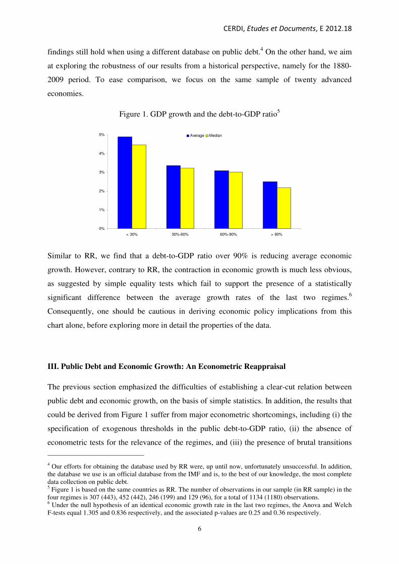
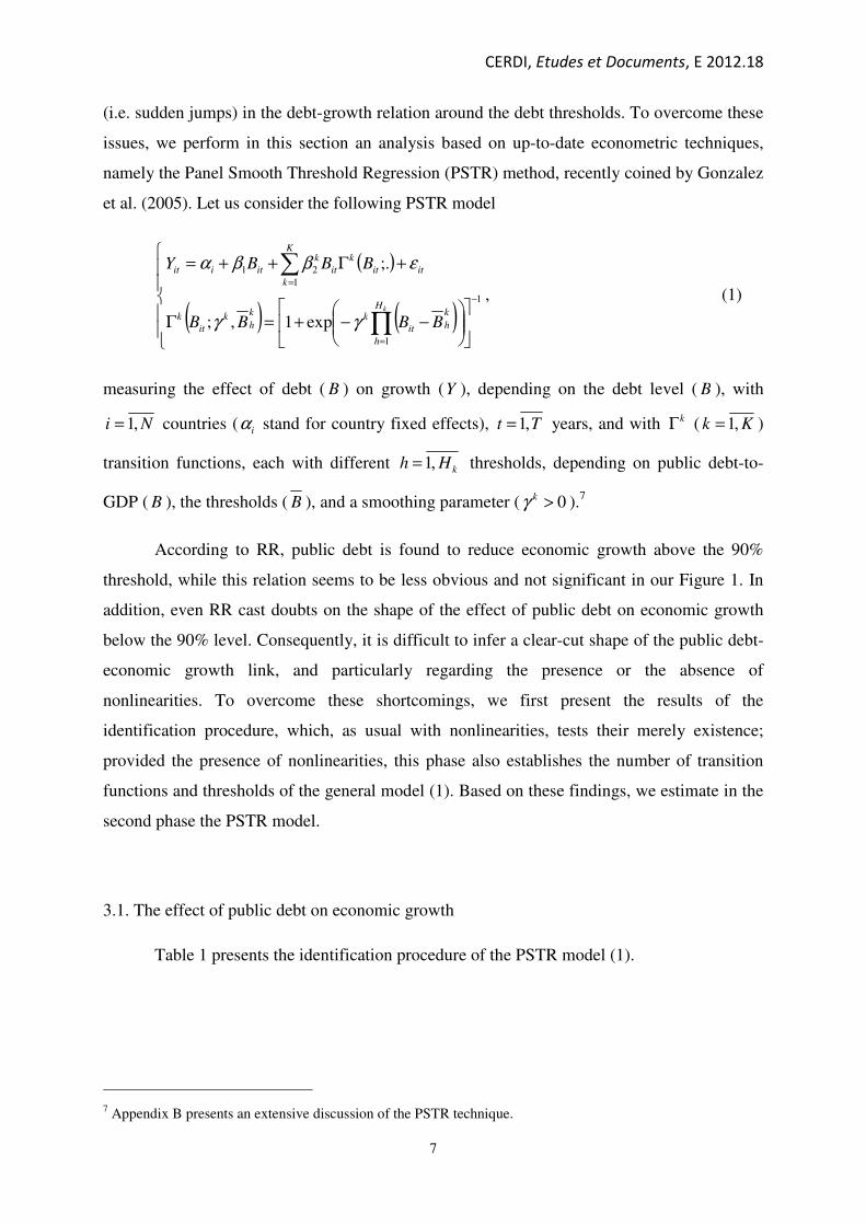
Figure 1. GDP growth and the debt-to-GDP ratio5

Similar to RR, we find that a debt-to-GDP ratio over 90% is reducing average economic

growth. However, contrary to RR, the contraction in economic growth is much less obvious,

as suggested by simple equality tests which fail to support the presence of a statistically

significant difference between the average growth rates of the last two regimes.6

Consequently, one should be cautious in deriving economic policy implications from this

chart alone, before exploring more in detail the properties of the data.

III. Public Debt and Economic Growth: An Econometric Reappraisal

The previous section emphasized the difficulties of establishing a clear-cut relation between

public debt and economic growth, on the basis of simple statistics. In addition, the results that

could be derived from Figure 1 suffer from major econometric shortcomings, including (i) the

specification of exogenous thresholds in the public debt-to-GDP ratio, (ii) the absence of

econometric tests for the relevance of the regimes, and (iii) the presence of brutal transitions

4 Our efforts for obtaining the database used by RR were, up until now, unfortunately unsuccessful. In addition,

the database we use is an official database from the IMF and is, to the best of our knowledge, the most complete

data collection on public debt. 5 Figure 1 is based on the same countries as RR. The number of observations in our sample (in RR sample) in the

four regimes is 307 (443), 452 (442), 246 (199) and 129 (96), for a total of 1134 (1180) observations. 6 Under the null hypothesis of an identical economic growth rate in the last two regimes, the Anova and Welch

F-tests equal 1.305 and 0.836 respectively, and the associated p-values are 0.25 and 0.36 respectively.

0%

1%

2%

3%

4%

5%

< 30% 30%-60% 60%-90% > 90%

Average Median


7

(i.e. sudden jumps) in the debt-growth relation around the debt thresholds. To overcome these

issues, we perform in this section an analysis based on up-to-date econometric techniques,

namely the Panel Smooth Threshold Regression (PSTR) method, recently coined by Gonzalez

et al. (2005). Let us consider the following PSTR model

( )

( ) ( )

−−+=Γ

+Γ++=

−

=

=

∏

∑1

1

1

21

exp1,;

;.

kH

h

k

hit

kk

hk

it

k

it

K

k

it

k

it

k

itiit

BBBB

BBBY

γγ

εββα

, (1)

measuring the effect of debt ( B ) on growth (Y ), depending on the debt level ( B ), with

Ni ,1= countries ( iα stand for country fixed effects), Tt ,1= years, and with kΓ ( Kk ,1= )

transition functions, each with different kHh ,1= thresholds, depending on public debt-to-

GDP ( B ), the thresholds ( B ), and a smoothing parameter ( 0>kγ ).7

According to RR, public debt is found to reduce economic growth above the 90%

threshold, while this relation seems to be less obvious and not significant in our Figure 1. In

addition, even RR cast doubts on the shape of the effect of public debt on economic growth

below the 90% level. Consequently, it is difficult to infer a clear-cut shape of the public debt-

economic growth link, and particularly regarding the presence or the absence of

nonlinearities. To overcome these shortcomings, we first present the results of the

identification procedure, which, as usual with nonlinearities, tests their merely existence;

provided the presence of nonlinearities, this phase also establishes the number of transition

functions and thresholds of the general model (1). Based on these findings, we estimate in the

second phase the PSTR model.

3.1. The effect of public debt on economic growth

Table 1 presents the identification procedure of the PSTR model (1).

7 Appendix B presents an extensive discussion of the PSTR technique.


8

Table 1. Identification of the PSTR model (1): nonlinearities in the public debt ratio

First transition

Function

Second transition function

(First transition function has three thresholds)

1 threshold LM Test 44.6 (2.38e-011) 2.57 (0.109)

F Test 45.6 (2.33e-011) 2.52 (0.113)

2 thresholds LM Test 50.1 (1.34e-011) 5.29 (0.071)

F Test 25.7 (1.25e-011) 2.60 (0.075)


F Test 20.5 (6.17e-013) 2.90 (0.034)

The tests are based on the linearized form of model (1) (see Appendix B). We considered up to 3=H

thresholds, as suggested by Gonzalez et al. (2005). Bolded values signal the strongest rejection of the null

hypothesis (namely, a linear panel). p-values are reproduced in brackets. Since this is a sequential procedure, the

significance level (1% or 5%) is reduced after each sequence by a constant factor 5.0=τ (see Gonzalez et al.,

2005).

The first column of Table 1 depicts the values of the tests for the first transition

function with up to three thresholds, as suggested by Gonzalez et al. (2005). The low p-values

confirm the existence of strong nonlinearities in the effect of public debt on economic growth.

Moreover, both LM and F tests show that the strongest rejection of the null hypothesis

criterion (see Gonzalez et al., 2005) is consistent with a first transition function with 3=H

thresholds. Thus, we block the number of thresholds to three in this first transition function,

and search next for a second transition function. Irrespective of the number of thresholds

considered, the rejection of the null hypothesis arises for p-values largely lower than for the

first transition function, and in particular lower than half of the significance level considered

in the first sequence (namely, 1% or 5%, see Gonzalez et al., 2005). Consequently, the PSTR

model that comes out from the identification procedure consists of one transition function

with three thresholds, namely


9

( )

( ) ( )1

3

1

321

***

)016.0()013.0(

***

exp1067.0,415.0;with

.120.0119.0

−

=

−−+=====Γ

+Γ+−=

∏h

hitit

itititit

BBBBBB

BBY

γγ

ε

. (2)

The results of the PSTR regression (2) were estimated following the algorithm presented in

Appendix B, with standard errors (corrected for heteroskedasticity) reproduced in brackets,

and the stars ***

denoting the significance at the 1% level. In line with the results emphasized

in the identification procedure, the presence of a nonlinear relation between public debt and

economic growth is confirmed by the strong significance of the 2β coefficient.

Let us explore in the following the effect of the public debt ratio on growth, namely

( ) ( ) ( )( )1332213212

221 231. BBBBBBBBBBBBdB

dYititit +++++−Γ−Γ+Γ+= γβββ .(3)

According to (3), the influence of the level of public debt on economic growth transits

through a rather complex nonlinear way. To have a better look at these effects, we present in

Figure 2 a graphical representation of (3), based on results from regression (2).

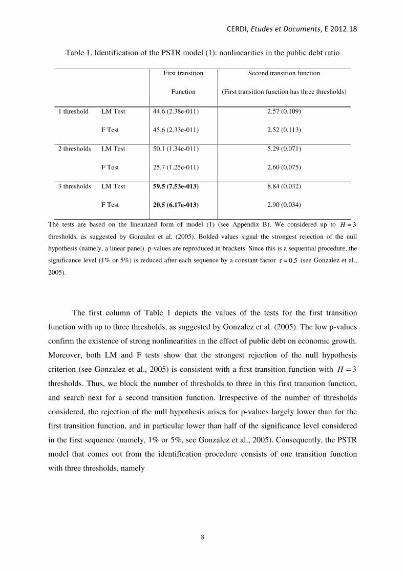
Figure 2. The effect of the public debt-to-GDP ratio on economic growth

The results depicted in Figure 2 confirm some of the findings of RR, and equally go

beyond them. Indeed, according to our estimations, an increase in the debt ratio decreases

economic growth (the derivative is negative). This result, which is in accordance with our

Figure 1 illustrating a negative correlation between economic growth and debt, extends the

analysis of RR who fail to derive a clear-cut relation between public debt and growth for debt

ratios below 90%. Besides, although economic growth declines as public debt increases, its

-0.08

-0.06

-0.04

-0.02

0

0.02

0.04

0.06

0.08

0.1

0% 30% 60% 90% 120% 150% 180% 210% 240% 270% 300%


10

reduction progressively vanishes, contrary to the conclusions of RR who support a dramatic

reduction in economic growth when public debt is above 90%.

Moreover, the effect of high (above 90%) public debt on growth displays much more

complex nonlinearities that stressed by RR. Indeed, an increase of public debt above the 90%

ratio reduces economic growth, as emphasized by RR. But in addition we depict the existence

of a threshold, around a public debt-to-GDP ratio of 115%, above which the correlation

between public debt and growth changes sign.8 Consequently, contrary to RR, countries with

public debt ratios above 90% not only do not see their economic growth plunging, but they

could even experience an increase in their growth, once public debt is above the

endogenously-estimated threshold of 115%.9

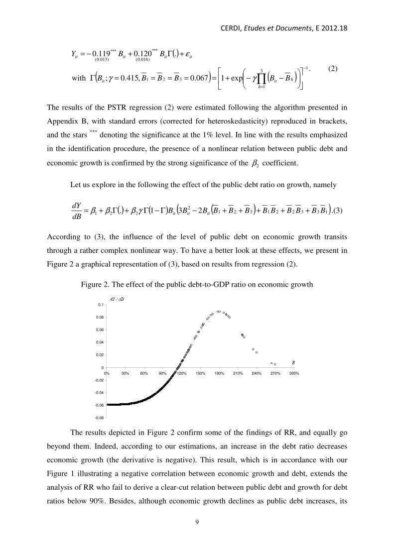
Figure 3 appends our Figure 1 above in light of these results, by accounting for the

presence of a threshold at around 115% for the public debt ratio (for simplicity, we focus on

public debt ratios above 60%).

Figure 3. GDP growth and the debt-to-GDP ratio: accounting for threshold effects

The first two charts, reproduced from our Figure 1, recall that average growth is lower

in countries with a public debt ratio above 90%, compared to countries with a debt ratio

between 60 and 90%.10

The last two charts develop the analysis by accounting for the

presence of threshold effects for a debt ratio of 115%; thus, we distinguish between high

8 Compared to RR, where the 90% debt threshold brutally distinguishes between countries with high,

respectively low growth rates, the transition between negative and positive effects of debt on growth occurs

smoothly, around the 115% debt threshold. 9 Besides, the magnitude of positive effect of public debt on economic growth is rather important, and may be

even stronger (in absolute value) than the negative effect illustrated for low public debt ratios. 10

However, remind that equality tests show that there is statistically no difference between average growth rates

for the two regimes.

0%

1%

2%

3%

4%

60%-90% > 90% 90%-115% > 115%

Average Median


11

public debt countries below this threshold (namely, with a debt ratio between 90 and 115%)

and respectively above it, and compute average and median economic growth rates.

In the spirit of RR, we find that compared to countries with a debt ratio between 60

and 90%, countries with a debt ratio between 90 and 115% experience a decline in their

average economic growth rates. Although this decline is statistically significant,11

notice that

the economic growth contraction is much less pronounced than acknowledged by RR. In

addition, contrary to RR, we find that countries with a public debt ratio above 115% present

an average growth rate which is higher compared to the average growth rate of countries with

a public debt ratio between 90 and 115%. More important, the growth rate of countries with a

debt ratio above 115% is not found to significantly decline compared to the growth rate of

countries with a debt ratio between 60 and 90% (the values of Anova and Welch mean

equality F-tests equal 0.169 and 0.050 respectively, and the associated p-values are 0.68 and

0.82 respectively).

3.2. Economic policy implications and robustness

Our findings reveal a different perspective in terms of economic policy

recommendations. Indeed, according to RR, countries should be cautious regarding their

fiscal policy, since loose fiscal policies, raising the public debt level, may drive them towards

high debt ratio regimes (characterized by a public debt above 90%), associated with

dramatically lower economic growth. Our results do not go against this general idea, since we

find that increasing public debt is detrimental to economic growth, when public debt is

relatively low. However, we also find that the negative effect of public debt on growth is

declining, and thus the growth contraction might be less important that acknowledged by RR.

In addition, we even show that raising public debt can even increase economic growth, in a

context of high debt levels, namely when the public debt-to-GDP ratio is above a threshold

level estimated at around 115%.

It is important to observe that we are not making the case for the use of loose fiscal

policies as an engine to promote economic growth, when public debt reaches high levels.

Instead, we aim at showing that an increasing public debt path is not generating bottomless pit

11 The values of Anova and Welch mean equality F-tests equal 4.568 and 6.250 respectively, and the associated

p-values are 0.03 and 0.01 respectively.


12

growth losses, but is bordered by a regime in which economic growth and debt may be

positively correlated. According to our analysis, countries in this regime, characterized by a

public debt-to-GDP ratio above 115%, present on average growth rates that are comparable to

the growth rates of countries with significantly lower public debt ratios, namely between 60

and 90%.

An immediate question regarding our findings concerns this last regime, namely

countries with high public debt ratios (above 115%) and high economic growth. Among them,

we can enumerate Belgium, Canada, New Zealand or United Kingdom, and the periods

concerned are the decade just after the WW2 and, to a lesser extent, the last decade of the 20th

century. However, one may argue that these events are singular, in the sense that they are not

likely to have been observed in other time periods; in this case, the positive association

between high public debt and growth may not be more but a simple artifact conditional to the

considered time sample. To tackle this critique, we aim at investigating if our results still hold

when considering a historical perspective. To this end, we perform our analysis on the same

sample of countries, but on the period 1880-2009, namely the double of the time length

considered previously (1945-2009).

The results of the identification procedure performed on the general PSTR model (1),

presented in Appendix A, support the presence of one transition function with one threshold.

The results of the estimation of this model are the following

( )

( ) ( )( )[ ] 1

11

)005.0(

***

)004.0(

***

exp1670.1,866.4;with

.031.0029.0

−−−+===Γ

+Γ+−=

BBBB

BBY

itit

itititit

γγ

ε, (4)

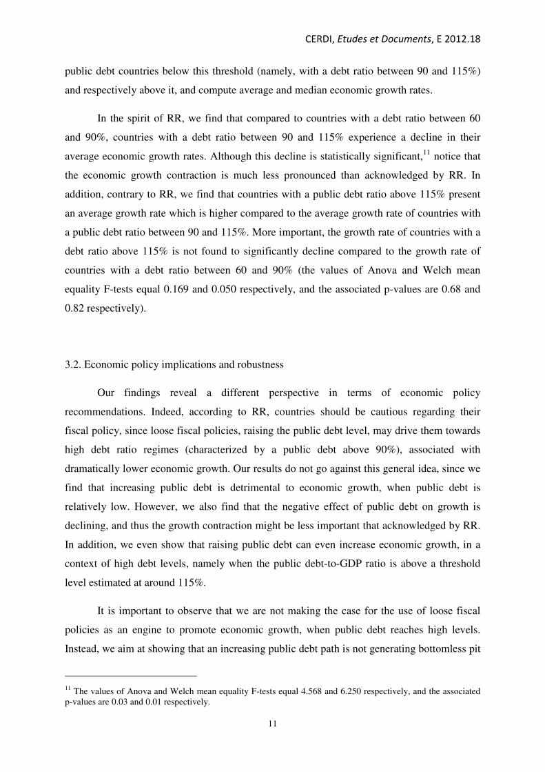
and the associated effect of public debt on economic growth is illustrated in Figure 4.


13

Figure 4. Public debt and economic growth in a historical perspective (1880-2009)

Figure 4 confirms that the results obtained for the 1945-2009 period are robust when

considering a historical perspective by looking at the relation between debt and growth over

the period 1880-2009. In particular, remark the presence, yet again, of a threshold for a public

debt-to-GDP ratio around 130%, above which the correlation between public debt and growth

becomes positive. In addition to the episodes emphasized above (for the 1945-2009 period),

this positive correlation can be also explained by historical events that occurred during the

1880-1945 period, and in particular by the “Roaring Twenties”. During this period, many

countries from our sample, including Belgium, France, Italy or UK, despite presenting

elevated (above our estimated threshold) public debt ratios, experienced remarkable high

economic growth rates.

Consequently, our analysis for the 1880-2009 period unveils two important facts. On

the one hand, we present an additional perspective on the outstanding period of the Roaring

Twenties, contributing to the fascinating existing literature on this topic (see, for example,

Schumpeter, 1946). On the other hand, we confirm that the positive association between debt

and growth is not singular to the recent period (1945-2009), but finds support from a

historical perspective.12

12 Besides, Appendix A confirms that economic growth is yet again statistically identical for countries with a

debt ratio between 60 and 90%, compared to countries with a debt ratio above the threshold of 130%.

-0.04

-0.03

-0.02

-0.01

0

0.01

0.02

0.03

0.04

0.05

0.06

0% 30% 60% 90% 120% 150% 180% 210% 240% 270% 300%


14

IV. Conclusion

This manuscript discusses one of the main results recently emphasized by the very influential

contribution of Reinhart & Rogoff (2010), namely the substantial economic growth decline

observed for advanced economies with a debt ratio above 90%. Using the new IMF database

on public debt, we show that, although higher public debt reduces growth for debt ratios

below the threshold considered by RR (namely 90%), this negative effect is declining as debt

increases. Moreover, we extend RR findings by emphasizing the presence of nonlinearities in

the effect of debt on growth for debt ratios above 90%. On the one hand, debt still reduces

growth for countries with a debt-to-GDP ratio below a threshold estimated at around 115%, as

acknowledged by RR. On the other hand, we reveal that economic growth and public debt are

positively associated for debt ratios above 115%; for countries in this regime, simple equality

tests support that average economic growth is not significantly different from the average

growth rate of countries with a public debt ratio between 60 and 90%. In addition, this latter

finding is confirmed when adopting a historical perspective, namely when considering the

same panel of countries but for the 1880-2009 period.

The implications of our results should be considered with caution. In particular, one

should refrain from recommending the adoption of loose fiscal policies as an engine to foster

economic growth in a context of high public debt levels. In turn, our results extend the

conclusions of RR, by showing that an increasing public debt path is not generating

bottomless pit growth losses, but is bordered by a regime is which economic growth can be

positively correlated with high public debt levels.

Consequently, the present paper, revealing nonlinear effects of high public debt levels

on economic growth, emphasizes that further analysis regarding the mechanisms underlying

these nonlinearities is needed before drawing economic policy recommendations, all the more

in a high-debt context as the one currently experienced by an important number of countries

worldwide.


15

References

- Ali Abas S., Belhocine N., ElGanainy A., Horton M. [2010], “A Historical Public Debt

Database”, IMF wp #10/245.

- Gonzalez A., Terasvirta T., van Dijk D. [2005], “Panel Smooth Transition Regression

Models”, Stockholm School of Economic wp #604.

- Maddison A. [2007], The World Economy. Historical Statistics. OECD Publishing (updated

from Angus Maddison’s page on the GGD Center, www.ggdc.net/MADDISON).

- Parent A. [2012], “The Development and Aftermath of Financial Crises: A Critical Note on

This Time is Different: Eight Centuries of Financial Folly, by C. Reinhart and K. Rogoff”,

Cliometrica, forthcoming.

- Reinhart C., Rogoff K. [2010], “Growth in a Time of Debt”, The American Economic

Review, Vol. 100, N°2, pp. 573-8, May.

- Schumpeter J. [1946], “The American Economy in the Interwar Period: The Decade of the

Twenties”, The American Economic Review, Vol. 36, N°2, pp. 1-10, May.


16

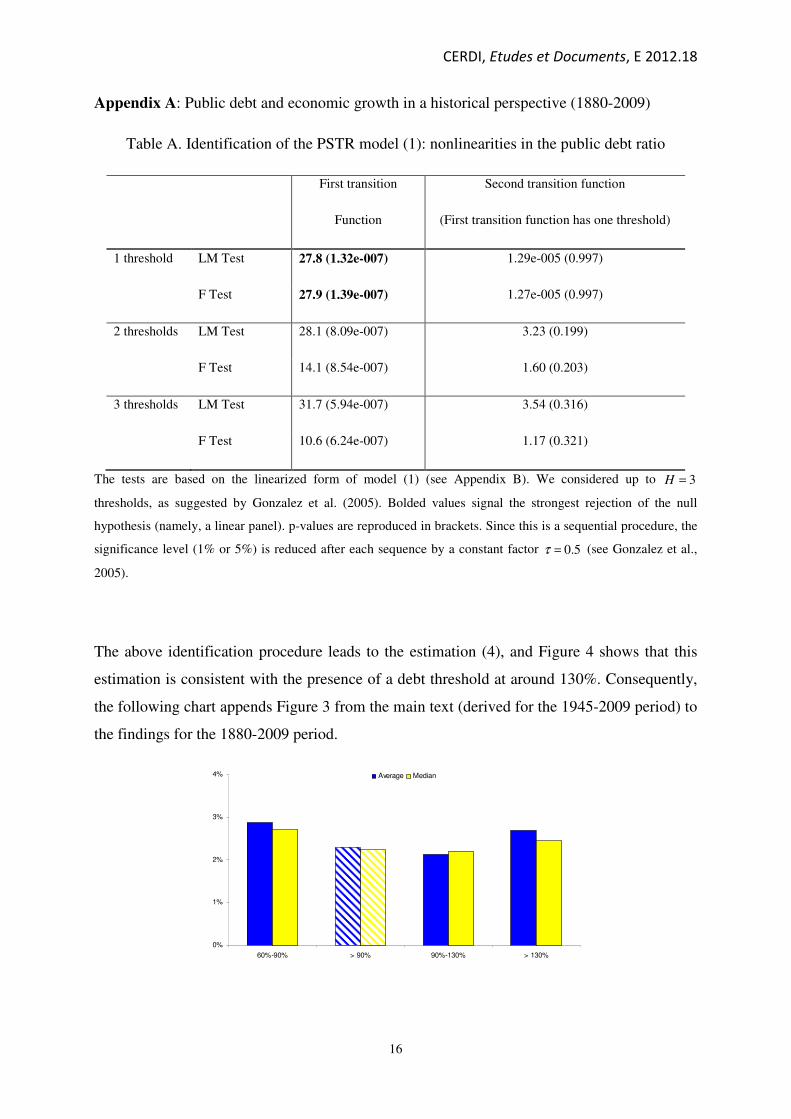
Appendix A: Public debt and economic growth in a historical perspective (1880-2009)

Table A. Identification of the PSTR model (1): nonlinearities in the public debt ratio

First transition

Function

Second transition function

(First transition function has one threshold)

1 threshold LM Test 27.8 (1.32e-007) 1.29e-005 (0.997)

F Test 27.9 (1.39e-007) 1.27e-005 (0.997)


F Test 14.1 (8.54e-007) 1.60 (0.203)


F Test 10.6 (6.24e-007) 1.17 (0.321)

The tests are based on the linearized form of model (1) (see Appendix B). We considered up to 3=H

thresholds, as suggested by Gonzalez et al. (2005). Bolded values signal the strongest rejection of the null

hypothesis (namely, a linear panel). p-values are reproduced in brackets. Since this is a sequential procedure, the

significance level (1% or 5%) is reduced after each sequence by a constant factor 5.0=τ (see Gonzalez et al.,

2005).

The above identification procedure leads to the estimation (4), and Figure 4 shows that this

estimation is consistent with the presence of a debt threshold at around 130%. Consequently,

the following chart appends Figure 3 from the main text (derived for the 1945-2009 period) to

the findings for the 1880-2009 period.

0%

1%

2%

3%

4%

60%-90% > 90% 90%-130% > 130%

Average Median


17

Simple equality tests show that (i) average growth declines for countries with a debt ratio

between 90 and 130% (the Anova and Welch mean equality F-tests equal 5.917 and 5.385,

and the associated p-values equal 0.01 and 0.02 respectively), and (ii) countries with high debt

ratios, namely above 130%, do not experience significantly different growth rates compared

to countries with a debt ratio between 60 and 90% (the Anova and Welch mean equality F-

tests equal 0.100 and 0.045, and the associated p-values equal 0.74 and 0.83 respectively).

These findings extend and confirm our conclusions for the 1945-2009 period.


18

Appendix B: A detailed presentation of the PSTR method

General considerations

The Panel Smooth Threshold Regression (PSTR) model, recently coined by Gonzalez

et al. (2005), can be seen as an upgrading of two existing techniques. On the one hand, as a

generalization to panel data of thresholds with smooth transition used in time series (see the

seminal paper on STAR models by Chan & Tong, 1986). On the other hand, as a

generalization to smooth transitions of panel threshold models (PTR) with brutal transitions.

In the following, we present the PSTR method in the light of the latter view.

PTR models were introduced by Hansen (1999), in an attempt for providing a tool for

estimating threshold effects on panel data. Indeed, recall that RR illustrate the presence of a

threshold at a debt-to-GDP ratio of 90%, above which growth declines dramatically.

Consequently, assuming a panel model of dimension Ni ,1= countries and Tt ,1= years, it is

appropriate to test the RR result in the following PTR model

( )

≥

<=Γ

+Γ++=

BBif

BBif

BBBBY

it

it

ititititiit

,1

,0(.)

;21 εββα

, (A1)

with iα country fixed effects, and itε an error term. According to (A1), the impact of the

public debt-to-GDP ratio B on the economic growth rate Y depends nonlinearly on the

values of the debt ratio with respect to the threshold B , namely 1/ β=dBdY if BBit <

(regime 1) and 21/ ββ +=dBdY if BBit ≥ (regime 2). If we follow RR, the threshold B

should be exogenously determined and equals to %90=B . However, Hansen (1999)

developed a procedure to endogenously estimate the value of the threshold B , as well as for

testing its relevance (namely, the absence of nonlinearities described by the null hypothesis

210 : ββ =H ) through a pertinent bootstrapping analysis. Besides, a sequential identification

procedure can be implemented to extend the PTR model to multiple thresholds.13

Despite its novelty compared to standard polynomial approaches for modeling

nonlinearities, the PTR model suffers however of two important shortcomings. First, the

13 As the number of thresholds increases, the estimation of the PTR model is technically more difficult (for

convergence issues, for example).


19

presence of a brutal transition between regimes, involving that either the elasticity fully

depends on the transition variable or is completely independent of it. This is the case in the

Figure 1 of RR, according to which the correlation between public debt and economic growth

is significantly different for countries with a public debt ratio on the left and respectively the

right hand side of the 90% threshold. However, such structural differences are hard to justify

for countries with fairly close public debt-to-GDP levels. Second, even if we develop (A1) to

the presence of multiple thresholds, the obtained PTR model would still allow for a reduced

number of regimes. For example, a two-threshold PTR model yields three different regimes

(i.e. three different elasticities), which may be considered as rather limited when one deals

with panel data with (i) an important time dimension (in this paper, 65 and up until 130

years), and (ii) important heterogeneity among countries (since the large time period we

consider may cover different stages of economic development). To overcome these

shortcomings in an adequate manner, we focus in the following on the PSTR technique.

Keeping the same notations as in (A1), let us assume the following PSTR model (the

model described by equation (1) in the main text)

( )

( ) ( )

−−+=Γ

+Γ++=

−

=

=

∏

∑1

1

1

21

exp1,;

;.

kH

h

k

hit

kk

hk

it

k

it

K

k

it

k

it

k

itiit

BBBB

BBBY

γγ

εββα

, (A2)

with kΓ ( Kk ,1= ) transition functions depending on the level of the public debt-to-GDP ratio

( B ), the threshold ( B ), and the smoothing parameter ( 0>kγ ) to be discussed below. In this

general formulation, we consider that each transition function kΓ has different kHh ,1=

thresholds.

The properties of the transition function, and of the PSTR model, crucially depend

upon the (non-negative) transition parameter γ . Indeed, when 0=γ , the transition function is

constant (it equals 0.5), and the PSTR model collapses to a linear model (since the dBdY /

elasticity does not depend on the level of the public debt ratio B anymore). In the other

extreme case ( ∞→γ ), the transition function takes only two independent values, and the

PSTR model collapses to a PTR model with brutal transition between regimes.14

Moreover,

14 Consequently, the PTR model may be viewed as a special case of a PSTR model, namely when ∞→γ .


20

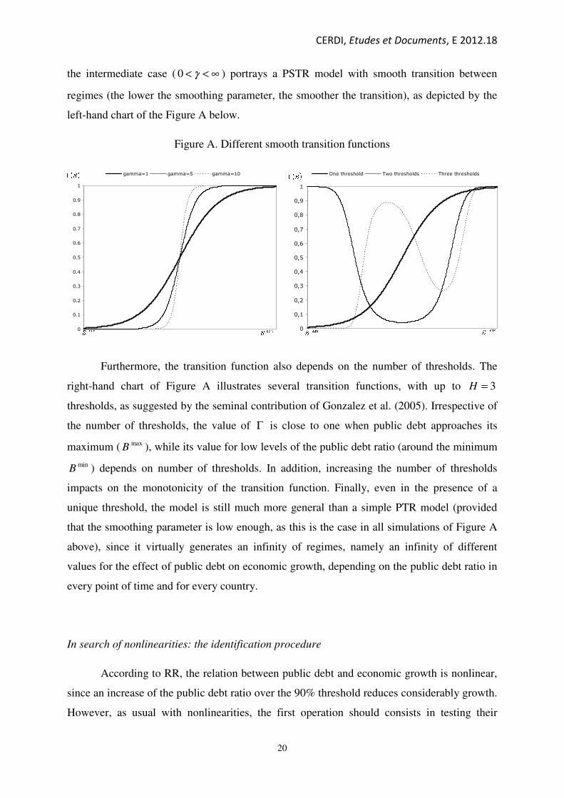
the intermediate case ( ∞<< γ0 ) portrays a PSTR model with smooth transition between

regimes (the lower the smoothing parameter, the smoother the transition), as depicted by the

left-hand chart of the Figure A below.

Figure A. Different smooth transition functions

Furthermore, the transition function also depends on the number of thresholds. The

right-hand chart of Figure A illustrates several transition functions, with up to 3=H

thresholds, as suggested by the seminal contribution of Gonzalez et al. (2005). Irrespective of

the number of thresholds, the value of Γ is close to one when public debt approaches its

maximum ( maxB ), while its value for low levels of the public debt ratio (around the minimum

minB ) depends on number of thresholds. In addition, increasing the number of thresholds

impacts on the monotonicity of the transition function. Finally, even in the presence of a

unique threshold, the model is still much more general than a simple PTR model (provided

that the smoothing parameter is low enough, as this is the case in all simulations of Figure A

above), since it virtually generates an infinity of regimes, namely an infinity of different

values for the effect of public debt on economic growth, depending on the public debt ratio in

every point of time and for every country.

In search of nonlinearities: the identification procedure

According to RR, the relation between public debt and economic growth is nonlinear,

since an increase of the public debt ratio over the 90% threshold reduces considerably growth.

However, as usual with nonlinearities, the first operation should consists in testing their

0

0.1

0.2

0.3

0.4

0.5

0.6

0.7

0.8

0.9

1

gamma=1 gamma=5 gamma=10

0

0,1

0,2

0,3

0,4

0,5

0,6

0,7

0,8

0,9

1

One threshold Two thresholds Three thresholds


21

merely existence. In a PTR setup, such tests suffer from a nuisance problem (see Hansen,

1999), which however may be overcome by an adapted bootstrapping procedure. Fortunately,

such complications may be avoided in a PSTR model; given that the transition function ( ).Γ

satisfies the necessary condition of continuity and presents sufficient conditions for

derivability, a simple way to check for the existence of nonlinear effects is to compute the

first-order Taylor-linearization of the transition function around the smoothing parameter

0→γ . For simplicity, consider a simple one-transition function one-threshold model

( )

( ) ( )( )[ ]

−−+=Γ

+Γ++=−1

21

exp1,;

;.

BBBB

BBBY

itit

ititititiit

γγ

εββα.

(A3)

Using the first-order linearization, namely ( ) ( ) 4/5.00.; BBit −+=→Γ γγ , (A3) becomes

≡−+≡

+++=

4/;4/5.0 2

*

2221

*

1

2*

2

*

1

γββγββββ

εββα

B

BBY itititiit. (A4)

Under this transformation, the PSTR model (A3) collapses to a simple second-order

polynomial nonlinear panel model. Moreover, since *

2β is a multiple of γ , we can test the

absence of nonlinearities in the PSTR model ( 0:0 =γH ) using the test 0:*

20 =βH . This

result also holds in the presence of two thresholds, as the parameters associated respectively

with 2B and 3B in the linearized model are also multiples of γ .15

To check for the existence

of such nonlinearities, we use the two tests developed by the related literature, namely the

Lagrange Multiplier-based (LM) test and its Fisher (F) version.16

To identify the structure of the PSTR model, we use the following cascade procedure.

In the first phase, we consider a PSTR model with one transition function, depending on up to

three thresholds. Based on the linearized form of the assumed PSTR model (A1) (or (1) in the

15 Namely, ( ) 4/212

*1

2 BB +−= γββ and 4/2

*2

2 γββ = respectively. In this case, the absence of nonlinear effects

0:0 =γH can be checked based on a joint nullity test 0: *2

2

*1

20 == ββH . The algebra for a model with three

thresholds is easily computable and available upon request. 16

Denoting by 0S and

1S the sum of squared residuals under the null hypothesis (linear panel) and the

alternative hypothesis (PSTR model) respectively, the tests are computed as ( ) 110 / SSSTNLM −= and

( )[ ] ( )[ ]HNTNSHSSF −−−= /// 110 (under the null hypothesis, LM follows a ( )Hχ distribution, while F

follows a ( )HNTNHF −−, distribution).


22

main text), we compute the above-mentioned linearity tests, for each number of thresholds.

Following Gonzalez et al. (2005), the number of thresholds for the first transition function is

chosen according to the strongest rejection of the null hypothesis (linear model). Once the

number of thresholds for the first transition function identified, we check, in phase two, for

the presence of a second transition function again with up to three thresholds. The procedure

stops when the null hypothesis of linear effects can no longer be rejected. Consequently,

contrary to traditional polynomial forms used to account for nonlinearities, this identification

procedure puts no ex-ante constraint on the functional form of the nonlinear relations. Indeed,

given the possibility of virtually combining multiple transition functions, with as much as

three thresholds for each one of them, provides sufficient place for obtaining dBdY /

elasticities that can depend in a rather complex manner on the level of the public debt-to-GDP

ratio.

The estimation of a PSTR model

At the end of the identification procedure, the number of transition functions, as well

as the number of thresholds for each transition function, is known. Next, we proceed to the

estimation of the PSTR model (i.e. the threshold(s), the transition parameter(s), and the

slopes), in a three-step procedure. For convergence issues, the first step consists of

eliminating fixed effects, an operation which, contrary to a traditional linear panel model, can

lead to some complications.17

Since the quality of the initial values for the parameters γ and

hB is crucial for the convergence of the estimation, the second step focuses on this problem.

Among several available methods, we use a “grid search” technique, which consists in

generating combinations of vectors ( )hB;γ , with arbitrary strictly positive γ -values and hB -

values from the sample. For each vector, we use the traditional panel least squares technique

to estimate the elasticities 2;1β , as well as the associated sum of squared residuals, which we

employ to find the vector of initial values for ( )hB;γ , as the one minimizing the sum of

17 To eliminate fixed effects, all variables of the model (A1) (or (1) in the main text) are centered as usual around

their means, except for the term including the transition function ( ) ( ).. Γ≡ itBG , which becomes: ( ) ( ) ( )...~

GGG −=

, with ( ) ( ) ( )( )∑∑=

−

=

− Γ==T

t

it

T

t

BTGTG1

1

1

1 ... . Consequently, the centered variable ( ).~G , used in the PSTR model

without fixed effects, depends on the γ and hB parameters in both ( ).G and ( ).G , which is why G~

must be

computed at each iteration, i.e. each time that γ and hB take different values.


23

squared residuals. The third and last step of the algorithm consists in estimating the PSTR model using the

Non-Linear Least Squares (NLLS) technique, based on iterations and consequently strongly dependant on the

quality of the initial values. The final estimators for the parameters ( )hB;γ are the one that minimize the

variance of residuals in the NLLS regression, and are being used in the panel least squares regression to estimate

the slopes 2;1β .

Supplementary references for Appendix B

- Chan, K., Tong, H. (1986), “On estimating thresholds in autoregressive models”, Journal of Time

Series Analysis 7, 179-190.

- Hansen, B., (1999), “Threshold effects in non-dynamic panels: Estimation, testing, and inference”,

Journal of Econometrics 93, 345-368.