Working Paper Series

Is Fair Trade Honey Sweeter? An empirical analysis on the effect of affiliation on productivity

Leonardo Becchetti Stefano Castriota

ECINEQ WP 2008 – 104

2

ECINEQ 2008-104 December 2008

www.ecineq.org

Is Fair Trade Honey Sweeter?

An empirical analysis on the effect of affiliation on productivity*

Leonardo Becchetti † University of Rome Tor Vergata

Stefano Castriota University of Trento

Abstract We evaluate the impact of affiliation to Fair Trade on a sample of Chilean honey producers. Evidence from standard regressions and propensity score matching shows that affiliated farmers have higher productivity (income from honey per worked hour) than the control sample. We show that the productivity effect is partially explained by the superior capacity of affiliated workers to exploit economies of scale. Additional results on the effects of affiliation on training, cooperation and advances on payments suggest that affiliation contributed both to, and independently from, the economies of scale effect. Keywords: Fair Trade, economies of scale, productivity. JEL Classification: D63, D64, O18, O19, O22.

* The authors thank for the discussion on fair trade issues F. Adriani, S. Anderson, M. Bagella, K Basu, F. Bourguignon, R. Cellini, L. Debenedictis, M. Fenoaltea, P. Garella, I. Hasan, L. Lambertini, S. Martin, C. McIntosh, N. Phelps, G. Piga and P. Scaramozzino, M E. Tessitore, P. Wachtel, C. Whilborg, H. White, B. Wydick and all participants of seminars held at the XV Villa Mondragone Conference, at SOAS in London, at the Copenhagen Business School and the Universities of Catania, Bologna, Macerata and Milano Bicocca, at the 2008 Poverty and growth network conference in Accra for the useful comments and suggestions received. The usual disclaimer applies. A Council of Rome grant is gratefully acknowledged. † Address of correspondence: Leonardo Becchetti, University of Rome Tor Vergata, Faculty of Economics,

Department of Economics and Institutions, Via Columbia 2, 00133 Rome Italy.

2

1. Introduction

Fair Trade (from now on also FT) may be considered as a general purpose

innovation which creates a new line of products. The main characteristic of such

products is that of being a bundle of physical and “socially responsible”

elements. The socially responsible content of FT goods consists of an original

organisation of the product chain and, within it, of the relationship between

primary producers, importers, certifiers and retailers. Such distinctive element

is formally resumed by FT (IFAT)2 rules. The latter documents how Fair Trade

schemes aim to use consumption and trade in order to promote inclusion and

capacity building of poor farmers in global product markets through a package

of benefits which include anti-cyclical mark-ups on prices, producer friendly

trade agreements (insurance against price fluctuations, advances on payments,

2 According to IFAT (the main federation gathering producers and Fair Trade organizations) such criteria are: i) Creating opportunities for economically disadvantaged producers; ii) Transparency and accountability; iii) Capacity building; iv) Promoting Fair Trade; v) Payment of a fair price; vi) Gender Equity; vii) Working conditions (healthy working environment for producers. The participation of children, if any, does not adversely affect their well-being, security, educational requirements and need for play and conforms to the UN Convention on the Rights of the Child as well as the law and norms in the local context); viii) The environment; ix) Trade Relations (Fair Trade Organizations trade with concern for the social, economic and environmental well-being of marginalized small producers and do not maximise profit at their expense. They maintain long-term relationships based on solidarity, trust and mutual respect that contribute to the promotion and growth of Fair Trade. Whenever possible, producers are assisted with access to pre-harvest or pre-production advance payment).

3

etc.), long-term relationships, credit facilities and business angel consultancy to

build producers’ capacity.

In recent times Fair Trade net sales have grown considerably, leading to a

mainstreaming of this market phenomenon from its original niche dimension.3

The reason for this success is the increasing willingness to pay of “concerned”

consumers for the social and environmental characteristics of the products.4 A

main problem in the “Fair Trade economy” is that the value creating intangible,

which represents its main innovation, cannot be tasted. This is because the

social and environmental content of FT products is not an experience good and

the asymmetric information problem between sellers and buyers may be only

partially solved with reputational mechanisms and the intermediation of

certifiers and labelling organisations.5

3 Between 2006 and 2007, total FT sales registered a 127% increase by volume and 72% by estimated retail value. Growth in Europe has averaged 50 % per year in the last 6 years. Even though Fair Trade has been originated by not for profit importers (ATOs), this impressive growth has induced traditional corporations to step in. Coop supermarkets in the UK and Italy created their own Fair Trade product lines since the ‘90es, Nestlè launched its first fair-trade product in 2005. In 2008 Tesco and Sainsbury announced their decision to sell 100% Fair Trade bananas leading the UK market share for this product to 25 percent (for a discussion on competition between fair trade dedicated retailers and supermarkets see also Kohler, 2007). On September the 3rd 2008 Ebay launched a dedicated platform (WorldOfGood.com) for fair trade e-commerce calculating that the U.S. market for such goods was $209 billion in 2005, and foreacasting that it will rise to $420 billion in 2010. 4 A recent inquiry on a representative sample of Italian consumers finds that around 30% of them are willing to buy FT products even if they have to pay up to 10% more with respect to non FT equivalent ones (Transfair, 2005). The share rises to around 70% when the price is the same. Similar results are found in other inquiries in the UK (Bird and Hughes, 1997), Belgium (De Pelsmacker, Driesen and Rayp, 2003) and Germany (www.fairtrade.net/sites/aboutflo/aboutflo). 5 Fairtrade Labelling Organizations International (FLO) is the umbrella organisation of 20 labelling Initatives in Europe as well as Canada, the United States, Japan, Australia and New Zealand. By the end of 2007, there were 632 Fair Trade certified producer organizations in 58 producing countries, representing 1.5 million farmers and workers. With their families and

4

Given the above mentioned framework, it is easy to understand the importance

of methodologically sound impact studies. They can be useful to importers to

evaluate, beyond the myth, whether all FT criteria are effectively applied and to

understand which factors are more beneficial in terms of producers’ inclusion

and capacity building. They can be useful to consumers to obtain more

information on the socially responsible content of the products and provide

sounder grounds to their willingness to pay.

The empirical literature of FT studies is growing and presents, togheter with

many valuable case studies (Bacon, 2005; Pariente, 2000; Castro, 2001a and

b; Nelson and Galvez, 2000; Ronchi, 2002 and 2006), some econometric

analyses which evaluate the impact of affiliation against the benchmark of a

control group of non FT producers living in the same areas (Ruben, 2009).

Among these papers Ronchi (2006) finds on a panel of 157 mill data that FT

helped affiliated Costa Rican coffee producers to increase their market power.

The author concludes that FT benefits are of the vertical integration type and

that “the decision to support fair trade requires other information about its

costs and benefits”. Becchetti and Costantino (2008) find that FT affiliates in

Kenya enjoy superior product and trade channel diversification, price stability

and insurance services. These effects generate social benefits in terms of

reduced child mortality, health and social capital (but no significant human

capital effects). Becchetti et al. (2008) observe in Peru that years of affiliation

dependents, FLO estimates that 7.5 million people directly benefit from Fairtrade. For further details see http://www.fairtrade.net/labelling_initiatives.html.

5

significantly increase productivity and self esteem. Consistently with the luxury

axiom (Basu, 1998 and 1999), effects on child schooling materialise only after

a given threshold of PPP income is overcome. These papers show that FT may

create positive or negative externalities in terms of changes of non affiliated

producers’ wellbeing and improved bargaining power of affiliated producers with

local intermediaries.

One of the limits of FT intervention, if not aimed at improving the capacity of

affiliated farmers to face market competition, is that it may create a form of

dependence from the (volatile) benevolence of socially responsible consumers.6

This is the reason why a more accurate empirical analysis (actually missing) on

the impact of FT affiliation on capacity building is of foremost importance. The

goal of our paper is to provide a contribution in this direction by analysing how

some specific characteristics of affiliation (anticipated payments, enhanced

interactions between producers and training courses) may affect productivity

and transition to the optimal scale of production.

The paper is divided as follows. In the second and third section we briefly

sketch the story of the cooperative of producers (Apicoop) affiliated to Fair

Trade and the dynamics of honey market, in the fourth section we present

descriptive statistics for the full sample and for the subsamples of affiliated and

6 The theoretical debate about pros and cons of Fair Trade revolves around three main points: the discussion on whether the price premium paid to producers is or is not a distortion of market clearing prices, the comparison of the relative efficiency/effectiveness of fair trade versus donations or subsidies, the externalities of Fair Trade introduction on other non affiliated local farmers (for details see Becchetti and Costantino, 2008; Maseland and De Vaal, 2002; Moore, 2004; Hayes, 2004 and Leclair, 2002).

6

non-affiliated producers. In the fifth section we focus on the effects of affiliation

on training courses, cooperation among producers and advances on payments.

In the sixth section we present and comment econometric results on

productivity. In the seventh section we deal with the selection bias problem.

The final section concludes.

2. History of Apicoop

During the military dictatorship of the ‘70s was very difficult and the Church

founded several organizations with the objective of helping the economic

development of the Dioceses. These institutions were usually financed with

foreign donations. For this reason, in 1980 Monsignor José Manuel Santos

founded Fundesval (FUNdación DESarrollo VALdivia) with capitals provided by

Miserior, a German institution founded in 1958 as agency "against hunger and

disease in the world"7.

Fundesval managed six different development projects, one of which was

related to honey.8 The honey-project pursued three objectives: (i) creating an

additional source of income to farmers; (ii) improving the feeding of the

population through the consumption of the honey produced; (iii) favoring the

7 www.miserior.de . 8Chile has a diverse variety of flowers of native species, herbaceous plants and trees that grow only in the central and southern areas of the country. One of these trees is ulmo, which stands out due to its pure white flowers, with extraordinary melliferous qualities. These flowers, so abundant as to make the tree appear covered in snow, are pollinated by bees that use the nectar to produce honey of ulmo, a speciality of northern Patagonia and of the Los Lagos region.

7

creation of a cooperative society (comité campesino). The first two targets were

reached within five years, while the third was realized only in 1998, when the

Diocese accepted the request of honey producers associated to the honey-

program to become independent. In fact, only the honey program was making

profits. The profits of the honey-program were used to cover the losses of the

others: on average, in the ‘80s around 28000-30000 USD were diverted every

year. Finally, in 1998 the honey producers took over the honey-program and

founded Apicoop, while the five remaining programs were closed.

In order to take over Fundesval, honey producers had to pay the Church a sum

of 180,000 USD in current terms. Furthermore, funds were needed to renovate

the main office, open the credit lines to farmers and buy new working tools.

The honey producers relied on the profits generated by their program in the

period 1998-1999, on a 50,000 USD loan provided by CTM Altromercato (an

Italian NGO which imports and sells Fair Trade products in Italy) and on two

donations of the Province of Bolzano (Northern Italy) which covered 50% of the

renovation costs of the ceiling of the office and of the honey collection room.

The decade 1998-2007 has been a long road towards financial independence

with the production of honey enormously increasing and Apicoop becoming the

fourth Chilean exporter of honey and the first Chilean producer of Fair Trade

honey. At present, the cooperative is made up of 127 beekeeping producers

partners (123 individuals and 4 cooperatives), distributed mostly in the Los

Lagos region. Apicoop members do not simply benefit from commercialization

8

of honey through the cooperative, but receive also free technical assistance, lab

tests on the quality of honey and interest-free credit support.

3. Evolution of prices and volumes in the Chilean export market of

honey

The honey market is subject to significant fluctuations in quantities and prices.

As a consequence of significant investments by farmers in Southern Chile, the

production and export of honey has increased enormously over the last years.

Fluctuations in export quantities and prices are due to sudden shocks to the

national production and to the international demand and supply.

A notewhorthy episode in this period is the sudden rise in the period 2002-2004

due to an antibiotic scandal which led the EU to ban the Chinese and

Argentinean honey for two years. Once, in 2005, imports from China and

Argentina were allowed again, the price fell by more than 40%. The current

positive price trend is due to the rising demand not only from developed

nations but also from developing ones. China, the biggest honey producer in

the world, has increased its per-capita consumption of honey thanks to the

rising purchasing power of its citizens, thereby contributing to the positive

trend. In such a complex international scenario, FT long-term contracts which

stabilize the revenues can be a good insurance for farmers.

4. Dataset and summary statistics

9

Evidence presented in the following sections comes from honey producers,

randomly sampled from two sets of treatment and control groups (respectively

farmers affiliated and not affiliated to Apicoop) and interviewed in January and

February 2008. The questionnaire consisted of a set of standard questions on

socio-demographic and economic variables, plus other questions related to the

honey production.9 The majority of honey producers are men, middle aged,

with primary or secondary education, married with children. Almost everybody

owns the house he lives in and some land (on average 10 hectares, ranging

from 0 to 160). One third of affiliated farmers have no more than 3 affiliation

years, while the top third of them more than 10.

The main activity is the production of honey (60% of the sample), but also

agriculture and other activities (usually employment in other firms) are

important. Worked hours are around 42 per week and approximately half of

them are devoted to the production of honey. Average annual total income is

five million Pesos (around 6,600 Euros or about 18 dollars per day).10 The

lowest values of total income and income from honey are equal to zero for

young people living with their family who are just starting the honey business.11

9 Table 1 describes the variables considered while summary statistics for the whole sample are omitted for reasons of space and available upon request. 10 This standard of living is far higher than what found in other Fair Trade impact studies. Becchetti and Costantino (2008) calculate a standard of living of around 3 dollars in PPP for Meru Herbs famers in Kenya. In Peru, Becchetti et al. (2008) find for the control samples of two producer groups in Juliaca and Chulucanas a standard of living of, respectively, around 0.6 and 6 dollars, against around 2 and 7 dollars for the corresponding samples of affiliated producers. 11 During the first years of activity all the productive effort is devoted to multiply the number of bee families and honey is not produced.

10

The simple unweighted average share of honey sold to the FT affiliated

cooperative (Apicoop) is equal to 50 percent, the retail share is 31 percent,

while shares of output sold to local or international intermediaries are lower

than 10 percent. The (wholesale) price of honey sold to the FT affiliated

cooperative is obviously lower than the retail price, but surprisingly is also

lower than the price paid by local, traditional and international intermediaries.

On the other hand, the cooperative provides a set of valuable services: free

transport of honey, zero interest advance payments, lab tests on honey

chemical properties, training courses, guaranted purchase of a given amount of

product which reduces producers’ search costs of buyers, etc.

The sample average production of honey per year is 3,200 kilos, but the

dispersion is high, ranging from 0 (3 new producers with no past yield records

met during the interviews)12 to 60,000, with a standard deviation of 6,100. The

average physical productivity (production per weekly hour of work devoted to

honey) is 180 kilos. Around 20 percent of producers get advanced payments,

whose average is 25 percent of the value of the honey production. Only one

individual out of 38 paid interests on the advances (at 20 percent rate), while

the others did not pay them since the cash in advance was provided by Apicoop

which does not charge anything for this service.

One quarter of the sample lives in towns and the remaining three quarters in

the countryside. The majority of individuals live in the area of Santa Barbara,

12 These producers are obviously eliminated from the productivity estimates which follow.

11

Rancagua, Paillaco and Mahiue, the remaining 45% being spread over several

villages.

Honey producers can be classified into three groups: people affiliated to FT

(which we call Flo producers), people not affiliated to FT (No Flo producers) and

people only indirectly affiliated to FT through another cooperative (Half Flo

producers). The first group is made of producers directly associated to the

cooperative. The second is made of producers not associated to the cooperative

who can, however, sell honey to the cooperative which, in turn, sells it locally.

Finally, people indirectly associated through other producer organizations may

sell to Apicoop and get the FT price and premium, but not the other services.

They are in between the Flo and the No Flo groups. The composition of our

sample is such that 46 % of respondents are directly associated to Apicoop,

12% indirectly through other organizations and 42% are independent.

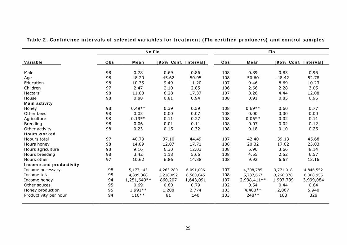
Table 2 shows means and confidence intervals of selected variables for the

subgroups of FT affiliated (Flo) and independent producers (No Flo). We do not

include the intermediate group (Half Flo) to focus on the difference between the

two extremes of full and no affiliation, but we will control for their

characteristics in the econometric estimates which follow. Double starred values

(**) indicate non overlapping confidence intervals, that is, 95 percent

significance of the difference in means between control and treatment groups.13

Although most socio-demographic characteristics are similar, there are

13 We run the Wilcoxon nonparametric rank test as a robustness check and obtain the same results in terms of significance. Evidence is omitted and available upon request.

12

important differences between the two subgroups, especially when looking at

the production of honey and at other economic variables.

The three main differences in performance between treatment and control

producers concern total yearly income from honey (2,998 against 1,252

thousand of pesos), the quantity of honey produced (4,403 against 1,991 kilos)

and productivity measured as income from honey per hour worked (248 against

110 pesos). This implies that affiliated producers are both larger in size and

more productive. One of the puzzles which we will try to disentangle is

therefore whether FT affiliation has additional benefits in terms of productivity,

net of the effect of size, and whether producers progressed in size and

economies of scale, also thanks to FT affiliation.

Since inclusion in one of the two (treatment and control) samples is non

random but depends on a voluntary choice of producers, we must control

whether differences between treated and non treated depend on implicit or

explicit selection bias. On the implicit side, producers’ characteristics which

affected the affiliation decision may also affect performance, irrespectively of

the affiliation effect. On the explicit side, it is reasonable to expect that the

cooperative selects the most promising candidates to meet the increasingly

high quality standards required by international competition. In 2006 this has

been made explicit in the statute of Apicoop which now establishes a set of

requisites to obtain membership. The most important of them states that the

applicant must have at least 3 years of proven production of honey and 25

13

beehives. Note however that, exactly for this record of increasing entry

standards, we should expect the performance gain to be decreasing in

affiliation years (since older producers belong to vintages with less stringent

quality requirements). An opposite result would, on the contrary, suggest that

this kind of selection bias cannot solely explain the observed differences.

From Table 2 we can see that productivity, production and income from honey

are significantly higher for Apicoop members. Our qualitative information from

cooperative members tells us that the training courses provided by the

association have surely played a role in increasing productivity, particularly

under the aspect of reducing bees’ diseases and increasing their honey

production. Econometric estimates will try to verify these declarations from a

quantitative point of view. On the contrary, the price and income per kilo sold

are lower for people associated to Apicoop since they produce higher amounts

and sell more wholesale (FT chain) rather than retail (local market).

Non affiliated producers sell only 7.5 percent of their production to Apicoop, 57

percent retail and the rest to local or international companies, while people

associated to Apicoop sell 82 percent to the cooperative, 14 percent to retail

and the remaining to other companies.14

The local retail price is lower for Apicoop’s members, thus there are no positive

externalities of FT affiliation on their bargaining power with local buyers.15

14 Apicoop’s statute imposes to their members to sell at least 80 percent of their production to them. 15 Evidence of such externality is provided in Becchetti et al. (2008) for Peruvian FT affiliated in the area of Juliaca (Titicaca lake).

14

Another surprising element is that the average salary paid by FT entrepreneurs

to the temporary workers is lower than that paid by independent ones. This is a

common problem with FLO and other FT organizations, whose rules and

statutes (see footnote 3) establish minimum prices and premiums for FT

members but do not deal with the relationship between producers and their

seasonal workers.

5. Training courses, advances of payments and Marshallian

externalities: the difference between affliated and non affiliated

producers

In this section we focus our attention on three qualifying differences between

affiliated and non affiliated farmers: advances on payments, attendance of

training courses and cooperation with local farmers. Looking at Table 2, only 2

percent of control sample farmers enjoy advances on payments against around

36 percent of Apicoop farmers. 44 percent of non affiliated farmers declare they

have not participated to training courses in the last three years, while this is

the case for only 22 percent of Apicoop farmers. 87 percent of Apicoop farmers

declare to cooperate with other producers in the area, while this occurs for 71

of non affiliated farmers. 95 percent confidence intervals show that these

differences in means are significant. Descriptive evidence on these three points

is confirmed by econometric analysis (see Table 3) where they are regressed on

15

a series of controls.16 The specifications include ender, schooling years, family

status dummies, number of family members, parents’ education, house

ownership, land size, total number of hours worked, geographical and type of

productive organization dummies.

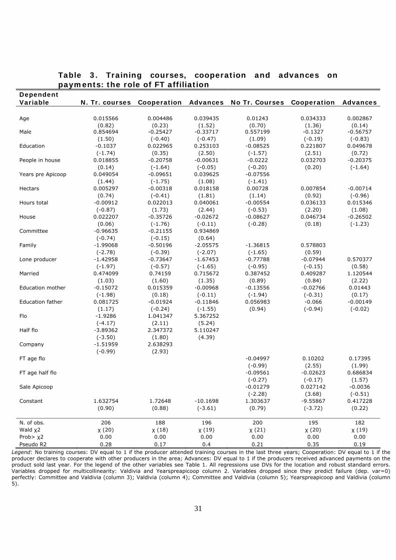
Our estimates show that affiliation to FLO certificated cooperatives is

significantly and negatively correlated with the probability of not having

participated to training courses in the last three years (such probability falls by

around 32 percent and by 27 percent for directly and indirectly affiliated

producers, respectively)17 (Table 3, column 1).18 The same direct affiliation is

positive and significant in regressions on the determinants of advances for

payment (marginal effect of 50 percent) and declaration to cooperate with

other local workers (marginal effect of 12 percent) (Table 3, columns 2 and 3).

Consider here that indirect affiliation has slightly higher effects in magnitude,

thereby showing that these two last benefits are already attainable with it.19

Cooperation is also positively and (weakly) significantly related to the number

of hours worked (.2 percent the marginal effect), while advances on payments

with schooling years. These associations are reasonable since hard working and

committed producers will be more likely, and have more opportunities, to

16 All estimates which follow are with White (1980) heteroskedasticity robust standard errors. 17 Marginal effect are not displayed in the estimates and calculated, following standad formulas, on the basis of estimated coefficients. 18 We introduce the two categories with separate regressors since we want to test the different effect of FT on affiliated and indirectly affiliated producers selling to Apicoop at FT conditions. 19 The first finding is consistent with the availability of all price benefits, also to indirectly affiliated producers selling to Apicoop for export in the FT channel.

16

interact with other producers, while more educated producers should possess

higher skills which produce superior creditworthiness.

The effect of FT affiliation has not just a once-for-all effect but also a

progressive one. When in our previous specification we replace the affiliation

dummy variable with two alternative measures of participation to the FT

channel (the length of the relationship with the cooperative and the production

share sold to the Apicoop cooperative) we find that years of relationship with

Apicoop have positive and significant effects on advances on payments and

cooperation with local workers (1 and 1.7 percent are the marginal effects of

one additional affiliation year on each of the two variables respectively) (Table

3, columns 4-6). Note as well that years of indirect affiliation (sales to Apicoop

without membership) have no significant effects confirming that part of the

benefits accrue only to fully affiliated producers.

Our findings are confirmed when we proxy closeness to the cooperative with

the share of producers’ output sold to Apicoop. The latter has negative

(positive) and significant effects on the probability of having never received

training courses (obtaining advances on payments) (-0.2 and 0.3 percent are,

respectively, the two effects for a one percent increase in the share of the

product sold to the cooperative).

The variable measuring local interactions among producers may be seen as a

proxy of Marshallian externalities if we consider the well known Marshall’s

17

definition.20 If we take into account standard criteria typically adopted in the

literature in order to define industrial districts21 we may observe that they apply

much more to the treatment than to the control sample. Considering the low

density and the geographical distance between producers in the rural areas in

which we run our survey, cooperative membership is one of the few

opportunities to bridge such distance and promote interactions among

producers.

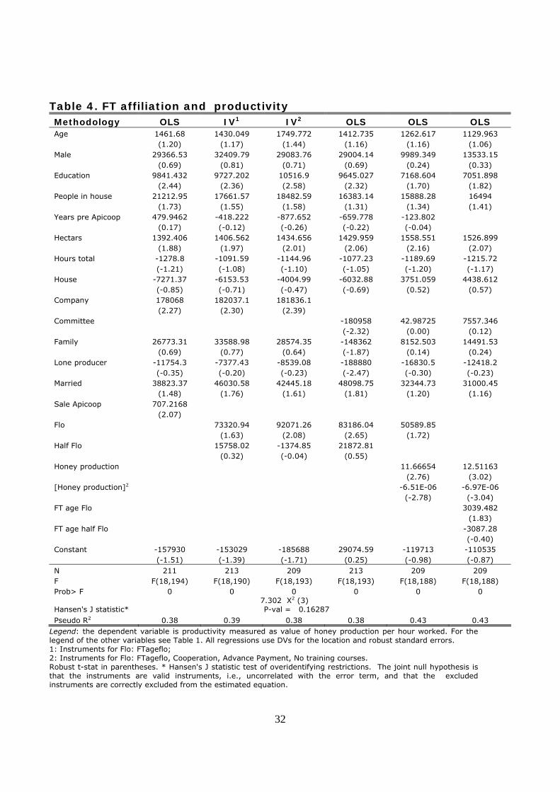
6. Productivity and FT affiliation

We measure productivity as income from honey production per hour worked

and regress it on measures of FT affiliation and various controls (Table 4,

columns 1-4). As it will be shown below, the first four specifications are model

free, while the two which follow test a specific theoretical assumption. The

estimate in column 4 shows that affiliation to FT is associated with an increase

20 “Industry’s secrets are ceasing to be secrets: they are, as it where, in the air and children are unwittingly learning many of them. Work well done is immediately recognised and people discuss right away the merits of inventions and improvements made to machines, processes and the general organisation of industry: if somebody comes up with a new idea, it is at once taken over by others and combined with their own home-made suggestions; it this becomes a source of other new ideas” (Marshall, 1920). 21 The main characteristics of industrial districts are generally considered to be: i) the concurring presence of cooperative and competitive features which reduce transaction costs, ii) the high horizontal and vertical mobility of workers (Becattini, 1990), iii) the abundance of exit and voice mechanisms generated by the intensity of productive relationships and interactions between firms and workers within the district (Brusco, 1982; Dei Ottati, 2000), iv) the local abundance of historically accumulated intangible production factors, from (managerial culture, know how, tacit capabilities) (Maillat, 1998), v) the presence of “social networks” (based on kinship, family and localness) which facilitate the flow of knowledge within district borders (Becattini, 1990). The presence of these socially homogeneous communities is expected to foster the intensity of inter-firm cooperation especially under the form of joint programs for the provision of collective goods (Paniccia, 1998) and of creation of local institutions (Lazerson and Lorenzoni, 1999), thereby increasing social capital, which is currently recognised as one of the crucial factors of growth and conditional convergence (Knack and Keefer, 1997).

18

of 83,186 pesos of honey income per hour worked. It is a remarkable difference

if we consider that average honey income per hour worked is 141,302 pesos.

Other significant factors are schooling years (9,645 pesos per additional year of

education), land size (1,429 pesos per hectar), type of productive organization

and (weakly) marital status.22 The link between our productivity variable and

affiliation is confirmed if, instead of the two dummy variables, we use a unique

synthetic indicator represented by the share of production sold to Apicoop

(Table 4, column 1). A one percent higher share of sales to Apicoop is

associated to a gain in farmer’s honey income per hour worked of 707 pesos.

The importance of the role of the three above described factors characterizing

affiliation (advances on payment, cooperation and training courses) is

confirmed when we instrument the affiliation dummy first with years of

affiliation (Table 4, column 2) and, after it, with the three factors (Table 4,

column 3). The instrumented variable is significant in the second but not in the

first case. The Hansen's J statistic test of overidentifying restrictions does not

reject the joint null hypothesis that the instruments are valid instruments, i.e.,

uncorrelated with the error term. We may wonder whether the affiliation effect

is due to the superior capacity of affiliated farmers to reap economies of scale.

We therefore make an explicit standard theoretical assumption on the inverse

U-shape of the average product function, which implies a U-shaped average

22 The significance of the affiliation variable persists if we limit the estimate to producers hiring seasonal workers and therefore include in the estimate cost of seasonal labour as an additional control. Estimates are omitted for reasons of space and available upon request.

19

cost function with increasing (decreasing) returns of scale in the downward

(upward) side of the curve. As a consequence, we estimate the following

specification:

∑++=j

jj XYYHY γβα 2/ with H0:α>0, β<0.

Consider as well that, if γj>0, this implies that the j-th factor (i.e. FT affiliation)

produces a significant perpendicular upward shift of the location of the affected

producer from the sample average product curve. Estimates in columns 5 and 6

show that the inverse U-shape assumption is not rejected (both levels and

squares of total output are significant and with the expected sign). However,

beyond size, years of affiliation (marginal effect of 3,039 pesos per year) and

schooling years have an independent positive effect on productivity (even

though they are now weakly significant). This implies that FT affiliation years

remain significant once we control for the productive scale. It is also interesting

to see that the affiliation effect materializes only for fully affiliated producers

(or the “FT age half flo” variable, measuring affiliation years of producers

selling to Apicoop at FT price conditions without being full cooperative

members, is not significant).

Two issues to be discussed in our results are omitted variable bias and

measurement error. As it is well known (Deaton, 1997) in development studies

the first problem generally relates to the quality of land23 and the second to

23 In this perspective, economies of scale may be a spurious effect driven by a downward bias of the size coefficient when the omitted quality variable is negatively related with size.

20

measuring income. Since we are looking at honey production, quality of land is

not so important, while quality of productive techniques is much more so. The

latter are not exogenous since they are affected by training courses and

interaction among local producers which, in turn, have been shown to be

affected by FT affiliation years. With regard to the measurement error problem,

the main candidate in our case is the dependent variable. This creates fewer

problems with respect to a measurement error in the regressors and should not

alter the sense of our estimates.

7. Controlling for selection bias: three approaches

An obvious problem in our model is the lack of dynamics which makes hard to

distinguish between the impact of FT affiliation and a selection bias effect. Does

affiliation improve productivity and economies of scale, or are more productive

and larger farmers more likely to enter the cooperative? We try to provide a

qualitative and two quantitative answers to this question. On a qualitative point

of view consider that the competitive race in export markets is becoming

progressively tighter and international standards of health and product quality

regulation increasingly more severe across years. It is therefore highly

implausible that Apicoop has affiliated progressively smaller and less efficient

producers across years.

Just to give an example of a “vintage” factor (invariant from the first affiliation

year to now) which should be correlated with productive skills at the moment of

21

entry, we find that average school years of producers with less than 3 years of

affiliation in 2007 are 10.44, against 8.37 of those between 6 and 9 years and

7.64 of those above 12 years. This descriptive finding seems consistent with

the progressively more severe (land size based) selection criteria described in

section 4, assuming the likely correlation between size and producer’s

education in the entry year.

Hence, the significant effect on a given performance variable of any additional

year of affiliation supports the hypothesis of a contribution from the

organization and acts against a (vintage driven) selection bias which should

operate in the opposite direction by reducing the positive, or even determining

a negative, link between years of affiliation and performance.

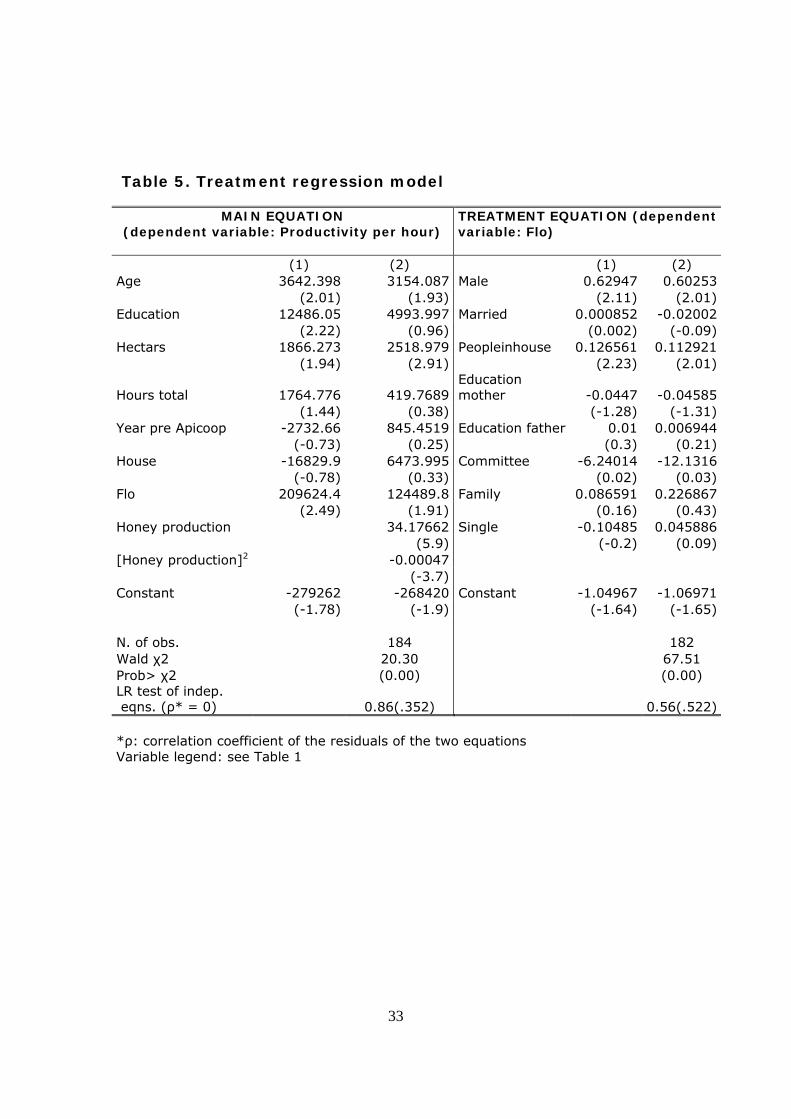
A first quantitative answer to the selection bias problem is provided by

estimating a treatment regression model in which the effect of FT affiliation is

controlled for the selection characteristics of affiliates. The treatment regression

model shown in Table 5 includes the following two equations24:

Honeyproductivityi = α0 + α1 Age + α2 Education + α3 Hectars + α4 HoursTotal

+ α5 YearspreApicoop + α6 House + α7 Flo + vi [1.1]

Floi = β0 + β1 Age + β2 Male + β3 Married + β4 PeopleInHouse + β5 Education

mother+ β6 Education father + Σk δk Prodstructurek + zi [1.2]

24 In the two equation system (v) and (z) are bivariate normal random variables with zero mean and covariance matrix

⎥⎦

⎤⎢⎣

⎡1ρρσ . The likelihood function for the joint estimation of [1.1] and

[1.2] is provided by Maddala (1983) and Greene (2003).

22

where Prodstructure are k dummies capturing the organizational form of the

producer (family, firm, committee,25 lone producer) and Regiondummies

capture regional location of the producer.

Note that, to meet the requirement of using selection variables not affecting

our performance indicator, in both estimates we use as regressors factors

which revealed themselves not correlated with the dependent variable in single

equation estimates. Some of these variables are however significant in the

selection equation (gender and firm organization). The hypothesis of

uncorrelation of residuals of the two equations is not rejected. The affiliation

variable remains significant both in the first and in a second specification in

which we control for economies of scale by adding the level and square of

honey production.

As a further robustness check we finally propose a second approach for

evaluating the effect of FT, net of the selection problem (Tables 6.1 and 6.2).

As it is well known, in the impossibility of having time series and applying more

sophisticated approaches,26 propensity score matching (PSM)27 may be a

reasonable approximation of it. By matching couples of treatment and control

producers which are closest in terms of selected characteristics, we may

assume with the PSM approach that the average treatment effect of the treated

25 The committee is an informal organization of a small group of individual producers who coordinate their sales and purchases of output in order to obtain higher bargaining power with local intermediaries. 26 Fair Trade existed in the area before our survey. Therefore it was impossible to perform a randomized experiment on the issue at stake in this paper. 27 For details on this approach see Dehejia and Wahba (2002), Heckman et al. (1996, 1998), Heckman, Ichimura, and Todd (1997, 1998). See Friedlander, Greenberg, and Robins (1997)

23

captures the specific contribution of FT affiliation on the selected performance

variable. Following what is standard in the literature when choosing regressors

to build the propensity score, we ensure that the vector of variables on which

the matching is conditioned is independent from individual assignement to the

treatment sample.

We also check that the second crucial condition (distribution of the outcome

conditioned on the set of independent variables from the treatment) is met.

Consider that our dependent variable is full affiliation and productive scale is

introduced among regressors. In this way we make our test more severe since

indirectly affiliated producers are in the control sample and the average

treatment effect is evaluated at the same level of productive scale.28 Obtained

findings confirm the difference between affiliated and non affiliated farmers

since average treatments of the treated (ATT or differences in means between

treatment and control samples) are significant when looking at share of product

sold to Apicoop, productivity (income from honey per hours worked), advances

on payments and cooperation with local farmers (Tables 6.1 and 6.2).29

28 Exclusion of indirectly affiliated producers from the test and elimination of the productive scale variables (level and squares of physical production) make differences between treatment and control sample more significant. Results are omitted for reasons of space and available upon request. 29 What the reader might question at this point is why not all producers choose affiliation given its benefits. The answer should be clear from our results. Less risk averse producers might prefer to take the risk of fluctuating honey prices to the implicit insurance provided by FT. Furthermore, affiliation to a cooperative implies the commitment to sell large part of their production to Apicoop and a series of social obligations that producers with a strong sense of independence may not like. Last but not least, producers not always have full awareness of the potential economic benefits of affiliation.

24

8. Conclusions

The recent literature on impact studies of FT affiliation is important in two

respects: i) it gives to consumers of FT products a test on the validity of the

promise to promote inclusion and wellbeing of marginalized producers, thereby

reducing the asymmetric information gap between consumers and sellers; ii) it

gives relevant insights to importers, labelers and retailers on the application of

criteria, emphasizing their strengths and weaknesses and stimulating their

discussion and implementation.

Our analysis on Chilean honey producers in a period of high market prices

highlights that, beyond the fair price myth, non price conditions are much more

important and capable of “Creating opportunities for economically

disadvantaged producers” as the first point of IFAT criteria announces. More

specifically, the case of Apicoop producers illustrates that FT affiliation, in spite

of an insignificant price differential in times of rising market prices, has helped

local farmers to improve their productive skills across years. In this process

more favourable financial conditions (advances on payments at 0% interest

rate), internalisation of Marshallian externalities via interactions among local

producers and training courses are the distinguishing features with respect to a

control sample of non affiliated producers which seem to have paid an

important role. On the overall, our findings show that affiliation years

significantly contribute to increase producers’ productivity shifting farmers

above the inverse U-shaped average product curve in the sample.

25

Among the limits which Fair Trade has to tackle we signal the need for more

transparency on full and half membership, the attention to wages of seasonal

employees of producers (which is not in the criteria) and the necessity to

increase awareness of local cooperative affiliates about Fair Trade.

References

[1] Bacon, C. (2005), “Confronting the Coffee Crisis: Can Fair Trade, Organic,

and Specialty Coffees Reduce Small-Scale Farmer Vulnerability in Northern Nicaragua?”, World Development, No. 33(3), pp. 497-511.

[2] Basu, K. (1999), “Child Labor: Cause, Consequence and Cure, with Remarks on International Labor Standards”, Journal of Economic literature, Vol. 37, pp. 1083-1119.

[3] Basu, K. & Van, P.H. (1998), “The Economics of Child Labor” American Economic Review, Vol. 88, pp. 412-427.

[4] Becattini, G., 1990, The Marshallian industrial district as a socio-economic notion, in F. Pyke et al. (eds.), Industrial district and Inter-firm cooperation in Italy, International Institute for Labour Studies, Geneva.

[5] Becchetti, L. & Costantino, M. (2008), “The Effects of Fair Trade on Marginalised Producers: an Impact Analysis on Kenyan Farmers, World Development, No. 36(5), pp. 823-842.

[6] Becchetti, L., Costantino, M. and Portale, E. (2008), “Human capital, externalities and tourism: three unexplored sides of the impact of FT affiliation on primary producers”, CEIS working paper No. 262.

[7] Bird, K. and D.R. Hughes (1997), “Ethical Consumption: The Case of ‘Fairly-Traded’ Coffee”, Business Ethics, No. 6(3), pp. 159-167.

[8] Brusco, S. (1982), “The Emilian Model: Productive Decentralization and Social Integration”, Cambridge Journal of Economics, Vol. 6 (2).

[9] Castro, J.E. (2001a), “Impact assessment of Oxfam's fair trade activities. The case of Productores de miel Flor de Campanilla”, Oxford: Oxfam.

[10] Castro, J.E. (2001b), “Impact assessment of Oxfam's fair trade activities. The case of COPAVIC”, Oxford: Oxfam.

[11] Deaton, A. (1997), “The Analysis of Household Surveys: A Microeconometric Approach to Development Policy”, The Johns Hopkins University Press (for the World Bank).

26

[12] Dehejia, R. H. & Wahba, S. (2002) “Propensity Score-Matching Methods for Nonexperimental Causal Studies”, The Review of Economics and Statistics,Vol. 84(1), pp. 151–161.

[13] Dei Ottati, G. (2000), “Exit, Voice, and Loyalty in the Industrial District: The Case of Prato”, University of Cambridge, ESRC Centre for Business Research, Working Paper WP175.

[14] De Pelsmacker P. & L. Driesen & G. Rayp (2003), "Are Fair Trade Labels Good Business? Ethics and Coffee Buying Intentions", Working Papers of Faculty of Economics and Business Administration, Ghent University.

[15] Friedlander D., Greenberg D. H. & Robins P. K., (1997), "Evaluating Government Training Programs for the Economically Disadvantaged," Journal of Economic Literature, Vol. 35(4), pp. 1809-1855.

[16] Greene, W. (2003), “Econometric Analysis”, 5th Edition, Prentice Hall. [17] Hayes, M. (2004), “Strategic Management Implication of the Ethical

Consumer”, www.fairtraderesearch.org. [18] Heckman, J., Ichimura, H. & Todd, P. (1997), “Matching as an

Econometric Evaluation Estimator: Evidence from Evaluating a Job Training Programme”, Review of Economic Studies, No. 64(4), pp. 605–654.

[19] Heckman, J., Ichimura, H. & Todd, P. (1998), “Matching as an Econometric Evaluation Estimator”, Review of Economic Studies, No. 65(2), pp. 261–294.

[20] Heckman et al. (1996), “Sources of Selection Bias in Evaluating Social Programs: An Interpretation of Conventional Measures and Evidence on the Effectiveness of Matching as a Program Evaluation Method”, Proceedings of the National Academy of Sciences, No. 93:23, pp. 13416–13420.

[21] Heckman et al. (1998), “Characterizing Selection Bias Using Experimental Data,” Econometrica, No. 66:5, pp. 1017–1098.

[22] Kohler P. (2007), “The Economics of Fair Trade: For Whose Benefit? An Investigation into the Limits of Fair Trade as a Development Tool and the Risk of Clean-Washing”, HEI Working Paper 06-2007.

[23] Knack, S. & Keefer, P. (1997), "Does Social Capital Have an Economic Payoff? A Cross-Country Investigation", Quarterly Journal of Economics, Vol. 112, pp. 1251-88.

[24] Leclair, M. S. (2002), “Fighting the Tide: Alternative Trade Organizations in the Era of Global Free Trade”, World Development, Vol. 30(7), pp. 1099–1122.

[25] Lazerson, M. H. & Lorenzoni, G. (1999), “The Firms that Feed Industial Districts: A Return to the Italian Source”, Industrial and Corporate Change, Vol. 8, pp. 36-47.

[26] Maddala, G. S. (1983), “Limited-Dependent and Qualitative Variables in Econometrics”, Econometric Society Monographs in Quantitative Economics, Cambridge University Press.

27

[27] Maillat, D. (1998), “From the Industrial District to the Innovative Milieu: Contribution to an Analysis of Territorialised Productive Organizations”, Recherches Economiques de Louvain, 64(1), pp. 111-129.

[28] Marshall, A. (1920), “Principles of Economics”, Macmillan, London. [29] Maseland, R. & De Vaal, A. (2002), “How Fair is Fair Trade?”, De

Economist, 150(3), 251-272. [30] Moore, G. (2004), “The Fair Trade Movement: Parameters, Issues and

Future Research”, Journal of Business Ethics, Vol. 53(1-2), pp. 73-86. [31] Nelson, V. & Galvez, M. (2000), “Social Impact of Ethical and

Conventional Cocoa Trading on Forest-Dependent People in Ecuador”. University of Greenwich, mimeo

[32] Paniccia, I. (1998), “One, a Hundred, Thousands of Industrial Districts”, Organization Studies, 19(4), pp. 667-699.

[33] Pariente, W. (2000), “The Impact of Fair Trade on a Coffee Cooperative in Costa Rica. A Producers Behaviour Approach”, Université Paris I Panthéon Sorbonne.

[34] Ronchi, L. (2002), “The Impact of Fair Trade on Producers and their Organizations: a Case Study with Coocafè in Costa Rica”, University of Sussex. mimeo

[35] Ronchi, L. (2006) "Fairtrade" and Market Failures in Agricultural Commodity Markets. World Bank Policy Research Working Paper 4011. Washington: IBRD.

[36] Ruben, R., (2009), The impact of fair trade, Wageningen Academic Publishers, Wageningen

[37] White, H. (1980), “A Heteroskedasticity-Consistent Covariance Matrix and a Direct test for Heteroskedasticity”, Econometrica, Vol. 48, pp. 817-38.

28

Table 1. Variables definition Variable Description Variable Description

Male DV equal to 1 if the respondent is male Sale to international intermediaries Share of honey sold to international intermediaries

Age Age in years Price Apicoop Price paid by Apicoop

Education Years of school attendance Price retail Retail price

Education mother Education of the mother in years Price local intermediaries Price paid by local intermediaries

Education father Education of the father in years Price traditional intermediaries Price paid by traditional intermediaries

Married DV equal to 1 if the respondent is married Price international intermediaries Price paid by international intermediaries

Single DV equal to 1 if the respondent is single Price per kilo Price of honey per kilo

Living together DV equal to 1 if the respondent lives with the partner Honey production Total production of honey in kilos

Divorced DV equal to 1 if the respondent is divorced Productivity per hour Value of honey prodution per hour worked

Separated DV equal to 1 if the respondent is separated Advance payment

DV equal to 1 if the respondent received advance payments

Widowed DV equal to 1 if the respondent is widowed Percentage advance Percentage of the value of the honey production received in advance

Children Number of children Interests on advance Interest rate applied to advance payments

People in house Number of people living in the household Training courses DV equal to 1 if the respondent attended training courses in the last 3 years

Hectars Property of land in hectars Loan DV equal to 1 if the respondent received a loan last year

House DV equal to 1 if the respondent owns the house Savings

DV equal to 1 if the respondent was able to save some money last year

Honey DV if honey is the main economic activity Credit restriction DV equal to 1 if the respondent faced credit restrictions last year

Other bees DV if other products from bees are the main economic activity Cooperation

DV equal to 1 if the producer declares to cooperate with other producers in the area

Agriculture DV if agriculture is the main economic activity Wage permanent worker

Average hourly wage of workers employed over the whole year

Breeding DV if breeding is the main economic activity Wage temporary worker Average hourly wage of seasonal workers

Other activity DV if the main economic activity is not one of those mentioned above Happiness Self declared happiness level (from 1 to 10)

Hours total Number of hours devoted to working activities in general Family satisfaction

Self declared satisfaction with economic conditions of the family (from 1 to 10)

Hours honey Number of hours devoted to the production of honey Town DV equal to 1 if the respondent lives in town

Hours agriculture Number of hours devoted to agriculture Santa Barbara DV equal to 1 if the respondent lives in Santa Barbara

Hours breeding Number of hours devoted to breeding Paillaco DV equal to 1 if the respondent lives in Paillaco

Hours other Number of hours devoted to other economic activities Rancagua DV equal to 1 if the respondent lives in Rancagua

Income necessary Income considered necessary to live well Mahiue DV equal to 1 if the respondent lives in Mahiue

Income total Total income earned last year Lone producer DV equal to 1 if the respondent produces honey alone

Income honey Income from honey last year Family DV equal to 1 if the respondent produces honey with the family

Income bees Income from other bees' products last year Company DV equal to 1 if the respondent created a company to produce honey

Income agriculture Income from agriculture last year Committee DV equal to 1 if the respondent belongs to a honey committee

Income breeding Income from breeding last year Years pre Apicoop Years of affiliation to a cooperative before the birth of Apicoop

Income other Income from other activities last year Flo DV equal to 1 if the respondent is directly associated to FT cooperatives

Other sources DV equal to 1 if the respondent has other sources of income

Half Flo

DV equal to 1 if the respondent is not affiliated to Apicoop but sells part of its production to Apicoop for the FT export channel enjoying the FT price benefits

Sale Apicoop Share of honey sold to Apicoop

No Flo

DV equal to 1 if the respondent is neither a Flo nor an Half Flo producer (not affiliated to Apicoop and not selling to Apicoop for the FT export channel)

Sale retail Share of honey sold to retail FT age flo Number of affiliation years of Apicoop members

Sale local intermediaries Share of honey sold to local intermediaries

FT age half flo

Number of years of trade relationships of non affiliated members selling to Apicoop for the FT export channel

Sale traditional intermediaries

Share of honey sold to traditional intermediaries

29

Table 2. Confidence intervals of selected variables for treatment (Flo certified producers) and control samples

No Flo Flo Variable Obs Mean [95% Conf. Interval] Obs Mean [95% Conf. Interval] Male 98 0.78 0.69 0.86 108 0.89 0.83 0.95 Age 98 48.29 45.62 50.95 108 50.60 48.42 52.78 Education 98 10.35 9.49 11.20 107 9.46 8.69 10.23 Children 97 2.47 2.10 2.85 106 2.66 2.28 3.05 Hectars 98 11.83 6.28 17.37 107 8.26 4.44 12.08 House 98 0.88 0.81 0.94 108 0.91 0.85 0.96 Main activity Honey 98 0.49** 0.39 0.59 108 0.69** 0.60 0.77 Other bees 98 0.03 0.00 0.07 108 0.00 0.00 0.00 Agriculture 98 0.19** 0.11 0.27 108 0.06** 0.02 0.11 Breeding 98 0.06 0.01 0.11 108 0.07 0.02 0.12 Other activity 98 0.23 0.15 0.32 108 0.18 0.10 0.25 Hours worked Hoours total 97 40.79 37.10 44.49 107 42.40 39.13 45.68 Hours honey 98 14.89 12.07 17.71 108 20.32 17.62 23.03 Hours agriculture 98 9.16 6.30 12.03 108 5.90 3.66 8.14 Hours breeding 98 3.42 1.18 5.66 108 4.55 2.52 6.57 Hours other 97 10.62 6.86 14.38 108 9.92 6.67 13.16 Income and productivity Income necessary 98 5,177,143 4,263,280 6,091,006 107 4,308,785 3,771,018 4,846,552 Income total 95 4,399,368 2,218,092 6,580,645 108 5,787,667 3,266,378 8,308,955 Income honey 94 1,251,649** 860,207 1,643,091 107 2,998,411** 1,997,739 3,999,084 Other souces 95 0.69 0.60 0.79 102 0.54 0.44 0.64 Honey production 95 1,991** 1,208 2,774 103 4,403** 2,867 5,940 Productivity per hour 94 110** 81 140 103 248** 168 328

30

Table 2. Confidence intervals of selected variables for treatment (flo certified producers) and control samples (follows)

No Flo Flo Variable Obs Mean [95% Conf. Interval] Obs Mean [95% Conf. Interval] Price, sales and financial conditions Sale Apicoop 98 7.50** 2.59 12.41 108 81.61** 77.10 86.12 Sale retail 98 56.87** 47.51 66.23 108 14.38** 10.32 18.44 Sale local intermediaries 98 11.42** 5.40 17.44 108 0.69** -0.10 1.49 Sale traditional intermediaries 98 18.17** 10.73 25.62 108 0.83** -0.08 1.75 Sale international intermediaries 98 1.76** -0.70 4.21 108 0.28** -0.27 0.83 Price Apicoop 10 754 720 788 101 764 753 774 Price retail sales 67 1,663** 1,565 1,761 70 1,461** 1,368 1,554 Price local intermediaries 20 818 730 905 3 1,533 -64 3,130 Price traditional intermediaries 14 792 730 854 3 1,133 374 1,892 Price international intermediaries 2 915 -1,436 3,266 1 1,500 . . Loans 98 0.70 0.61 0.80 105 0.80 0.72 0.88 Savings 97 0.55 0.45 0.65 108 0.57 0.48 0.67 Wage permanent 2 850 -3,597 5,297 10 822 575 1,069 Wage temporary 36 1,012** 906 1,117 45 843** 789 897 Cooperative services Never attended training courses 98 0.438** 0.338 .5387. 86 .244** .151 .336 Cooperation 98 0.714** 0.623 0.805 87 .873** .802 .944 Advance payment 94 0.02** -0.01 0.05 107 0.36** 0.26 0.45 Percent advance 1 10** . . 35 23.20** 16.93 29.47 Interests on advance 1 20** . . 32 0.09** -0.10 0.28

**: the difference in mean among the two groups is significant at 5% level. Producers only indirectly affliated to Apicoop (Half Flo) are ruled out from the sample in order to focus on differences between full and no affiliation.

31

Table 3. Training courses, cooperation and advances on payments: the role of FT affiliation

Dependent Variable N. Tr. courses Cooperation Advances No Tr. Courses Cooperation Advances Age 0.015566 0.004486 0.039435 0.01243 0.034333 0.002867 (0.82) (0.23) (1.52) (0.70) (1.36) (0.14) Male 0.854694 -0.25427 -0.33717 0.557199 -0.1327 -0.56757 (1.50) (-0.40) (-0.47) (1.09) (-0.19) (-0.83) Education -0.1037 0.022965 0.253103 -0.08525 0.221807 0.049678 (-1.74) (0.35) (2.50) (-1.57) (2.51) (0.72) People in house 0.018855 -0.20758 -0.00631 -0.0222 0.032703 -0.20375 (0.14) (-1.64) (-0.05) (-0.20) (0.20) (-1.64) Years pre Apicoop 0.049054 -0.09651 0.039625 -0.07556 (1.44) (-1.75) (1.08) (-1.41) Hectars 0.005297 -0.00318 0.018158 0.00728 0.007854 -0.00714 (0.74) (-0.41) (1.81) (1.14) (0.92) (-0.96) Hours total -0.00912 0.022013 0.040061 -0.00554 0.036133 0.015346 (-0.87) (1.73) (2.44) (-0.53) (2.20) (1.08) House 0.022207 -0.35726 -0.02672 -0.08627 0.046734 -0.26502 (0.06) (-1.76) (-0.11) (-0.28) (0.18) (-1.23) Committee -0.96635 -0.21155 0.934869 (-0.74) (-0.15) (0.64) Family -1.99068 -0.50196 -2.05575 -1.36815 0.578803 (-2.78) (-0.39) (-2.07) (-1.65) (0.59) Lone producer -1.42958 -0.73647 -1.67453 -0.77788 -0.07944 0.570377 (-1.97) (-0.57) (-1.65) (-0.95) (-0.15) (0.58) Married 0.474099 0.74159 0.715672 0.387452 0.409287 1.120544 (1.03) (1.60) (1.35) (0.89) (0.84) (2.22) Education mother -0.15072 0.015359 -0.00968 -0.13556 -0.02766 0.01443 (-1.98) (0.18) (-0.11) (-1.94) (-0.31) (0.17) Education father 0.081725 -0.01924 -0.11846 0.056983 -0.066 -0.00149 (1.17) (-0.24) (-1.55) (0.94) (-0.94) (-0.02) Flo -1.9286 1.041347 5.367252 (-4.17) (2.11) (5.24) Half flo -3.89362 2.347372 5.110247 (-3.50) (1.80) (4.39) Company -1.51959 2.638293 (-0.99) (2.93) FT age flo -0.04997 0.10202 0.17395 (-0.99) (2.55) (1.99) FT age half flo -0.09561 -0.02623 0.686834 (-0.27) (-0.17) (1.57) Sale Apicoop -0.01279 0.027142 -0.0036 (-2.28) (3.68) (-0.51) Constant 1.632754 1.72648 -10.1698 1.303637 -9.55867 0.417228 (0.90) (0.88) (-3.61) (0.79) (-3.72) (0.22) N. of obs. 206 188 196 200 195 182 Wald χ2 χ (20) χ (18) χ (19) χ (21) χ (20) χ (19) Prob> χ2 0.00 0.00 0.00 0.00 0.00 0.00 Pseudo R2 0.28 0.17 0.4 0.21 0.35 0.19

Legend: No training courses: DV equal to 1 if the producer attended training courses in the last three years; Cooperation: DV equal to 1 if the producer declares to cooperate with other producers in the area; Advances: DV equal to 1 if the producers received advanced payments on the product sold last year. For the legend of the other variables see Table 1. All regressions use DVs for the location and robust standard errors. Variables dropped for multicollinearity: Valdivia and Yearspreapicoop column 2. Variables dropped since they predict failure (dep. var=0) perfectly: Committee and Valdivia (column 3); Valdivia (column 4); Committee and Valdivia (column 5); Yearspreapicoop and Valdivia (column 5).

32

Table 4. FT affiliation and productivity Methodology OLS IV1 IV2 OLS OLS OLS Age 1461.68 1430.049 1749.772 1412.735 1262.617 1129.963 (1.20) (1.17) (1.44) (1.16) (1.16) (1.06) Male 29366.53 32409.79 29083.76 29004.14 9989.349 13533.15 (0.69) (0.81) (0.71) (0.69) (0.24) (0.33) Education 9841.432 9727.202 10516.9 9645.027 7168.604 7051.898 (2.44) (2.36) (2.58) (2.32) (1.70) (1.82) People in house 21212.95 17661.57 18482.59 16383.14 15888.28 16494 (1.73) (1.55) (1.58) (1.31) (1.34) (1.41) Years pre Apicoop 479.9462 -418.222 -877.652 -659.778 -123.802 (0.17) (-0.12) (-0.26) (-0.22) (-0.04) Hectars 1392.406 1406.562 1434.656 1429.959 1558.551 1526.899 (1.88) (1.97) (2.01) (2.06) (2.16) (2.07) Hours total -1278.8 -1091.59 -1144.96 -1077.23 -1189.69 -1215.72 (-1.21) (-1.08) (-1.10) (-1.05) (-1.20) (-1.17) House -7271.37 -6153.53 -4004.99 -6032.88 3751.059 4438.612 (-0.85) (-0.71) (-0.47) (-0.69) (0.52) (0.57) Company 178068 182037.1 181836.1 (2.27) (2.30) (2.39) Committee -180958 42.98725 7557.346 (-2.32) (0.00) (0.12) Family 26773.31 33588.98 28574.35 -148362 8152.503 14491.53 (0.69) (0.77) (0.64) (-1.87) (0.14) (0.24) Lone producer -11754.3 -7377.43 -8539.08 -188880 -16830.5 -12418.2 (-0.35) (-0.20) (-0.23) (-2.47) (-0.30) (-0.23) Married 38823.37 46030.58 42445.18 48098.75 32344.73 31000.45 (1.48) (1.76) (1.61) (1.81) (1.20) (1.16) Sale Apicoop 707.2168 (2.07) Flo 73320.94 92071.26 83186.04 50589.85 (1.63) (2.08) (2.65) (1.72) Half Flo 15758.02 -1374.85 21872.81 (0.32) (-0.04) (0.55) Honey production 11.66654 12.51163 (2.76) (3.02) [Honey production]2 -6.51E-06 -6.97E-06 (-2.78) (-3.04) FT age Flo 3039.482 (1.83) FT age half Flo -3087.28 (-0.40) Constant -157930 -153029 -185688 29074.59 -119713 -110535 (-1.51) (-1.39) (-1.71) (0.25) (-0.98) (-0.87) N 211 213 209 213 209 209 F F(18,194) F(18,190) F(18,193) F(18,193) F(18,188) F(18,188) Prob> F 0 0 0 0 0 0

Hansen's J statistic* 7.302 Χ2 (3) P-val = 0.16287

Pseudo R2 0.38 0.39 0.38 0.38 0.43 0.43 Legend: the dependent variable is productivity measured as value of honey production per hour worked. For the legend of the other variables see Table 1. All regressions use DVs for the location and robust standard errors. 1: Instruments for Flo: FTageflo; 2: Instruments for Flo: FTageflo, Cooperation, Advance Payment, No training courses. Robust t-stat in parentheses. * Hansen's J statistic test of overidentifying restrictions. The joint null hypothesis is that the instruments are valid instruments, i.e., uncorrelated with the error term, and that the excluded instruments are correctly excluded from the estimated equation.

33

Table 5. Treatment regression model

MAIN EQUATION (dependent variable: Productivity per hour)

TREATMENT EQUATION (dependent variable: Flo)

(1) (2) (1) (2) Age 3642.398 3154.087 Male 0.62947 0.60253 (2.01) (1.93) (2.11) (2.01) Education 12486.05 4993.997 Married 0.000852 -0.02002 (2.22) (0.96) (0.002) (-0.09) Hectars 1866.273 2518.979 Peopleinhouse 0.126561 0.112921 (1.94) (2.91) (2.23) (2.01)

Hours total 1764.776 419.7689 Education mother -0.0447 -0.04585

(1.44) (0.38) (-1.28) (-1.31) Year pre Apicoop -2732.66 845.4519 Education father 0.01 0.006944 (-0.73) (0.25) (0.3) (0.21) House -16829.9 6473.995 Committee -6.24014 -12.1316 (-0.78) (0.33) (0.02) (0.03) Flo 209624.4 124489.8 Family 0.086591 0.226867 (2.49) (1.91) (0.16) (0.43) Honey production 34.17662 Single -0.10485 0.045886 (5.9) (-0.2) (0.09) [Honey production]2 -0.00047 (-3.7) Constant -279262 -268420 Constant -1.04967 -1.06971 (-1.78) (-1.9) (-1.64) (-1.65) N. of obs. 184 182 Wald χ2 20.30 67.51 Prob> χ2 (0.00) (0.00) LR test of indep. eqns. (ρ* = 0) 0.86(.352) 0.56(.522) *ρ: correlation coefficient of the residuals of the two equations Variable legend: see Table 1

34

Table 6.1 Differences among affiliated and non affiliated farmers (Propensity Score Matching)

Variable n.treat n.contr ATT* T-stat Honey per hour worked 87 119 1.02E+05 2.111 Cooperation with local producers 87 119 0.167 2.58 Comparative standard of living 87 119 0.438 1.436 Professional self-esteem 87 119 0.381 1.503 Advances on payments 87 119 0.242 3.309 Share sold to Apicoop 87 119 55.71 11.245

Note: ATT is the average treatment of the treated. Regressors in the ATT estimate: age, education, hectars, people in house, family, company, married, honey production and honey production squared. The balancing property is satisfied. Standard errors with bootstrapping and 50 replications. Table 6.2 Propensity score estimate (Dependent variable: Flo)

Regressor Coeff. T-stat Age -0.00195 -0.23 House -0.00465 -0.04 Male 0.499989 2.05 Company 0.029337 0.03 Family owned 0.364339 0.54 Single 0.185419 0.27 Married -0.26474 -1.18 Peopleinhouse 0.113956 2.32 Education mother -0.05083 -1.32 Education father 0.001631 0.05 Constant -0.95792 -1.14

N. of observations 176

LR χ2 (9) 25.43

Prob > χ2 0.002

Log likelihood -109.86812

Pseudo R2 0.0707

35

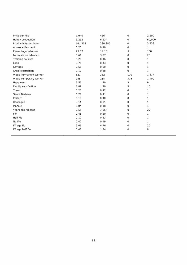
Appendix – not to be published Table A1. Summary Statistics of Socio-Demographic and Economic Variables

Variable OMean Std. Dev. Min Max Male 0.84 0.37 0 1

Age 49.74 12.70 24 88

Education 9.92 4.19 0 22

Education mother 4.56 4.01 0 16

Education father 4.66 4.27 0 18

Married 0.65 0.48 0 1

Single 0.20 0.40 0 1

Living together 0.09 0.28 0 1

Divorced 0.01 0.09 0 1

Separated 0.03 0.16 0 1

Widowed 0.03 0.18 0 1

People in house 3.97 1.82 1 12

Children 2.50 1.89 0 11

Hectars 9.60 22.82 0 160

House 0.87 0.34 0 1

Honey 0.61 0.49 0 1

Other bees 0.01 0.11 0 1

Agriculture 0.13 0.34 0 1

Breeding 0.06 0.25 0 1

Other activity 0.20 0.40 0 1

Hours total 42.26 17.54 2 105

Hours honey 18.33 14.28 0 70

Hours agriculture 7.55 13.45 0 60

Hours breeding 3.94 10.59 0 70

Hours other 9.93 17.34 0 89

Income necessary 4,784,549 3,605,721 480,000 36,000,000

Income total 4,988,680 11,400,000 0 110,000,000

Income honey 2,109,031 3,878,463 0 40,000,000

Income bees 346,100 1,016,250 0 10,000,000

Income agriculture 967,496 7,125,316 0 100,000,000

Income breeding 247,122 841,495 0 9,000,000

Income other 1,350,009 6,009,740 0 80,000,000

Other sources 0.61 0.49 0 1

Sale Apicoop 50.70 44.14 0 100

Sale retail 31.61 40.09 0 100

Sale local intermediaries 5.53 21.23 0 100

Sale traditional intermediaries 8.06 25.68 0 100

Sale to international intermediaries 0.86 8.18 0 92

Price Apicoop 767 51 600 950

Price retail 1,536 393 800 2,500

Price local intermediaries 904 352 680 2,000

Price traditional intermediaries 894 260 680 1,600

Price international intermediaries 1,110 385 730 1,500

36

Price per kilo 1,040 466 0 2,500

Honey production 3,232 6,134 0 60,000

Productivity per hour 141,302 280,286 0 3,333

Advance Payment 0.20 0.40 0 1

Percentage advance 25.07 19.13 5 100

Interests on advance 0.61 3.27 0 20

Training courses 0.29 0.46 0 1

Loan 0.76 0.43 0 1

Savings 0.55 0.50 0 1

Credit restriction 0.17 0.38 0 1

Wage Permanent worker 821 332 170 1,477

Wage Temporary worker 935 258 375 1,900

Happiness 5.55 1.70 3 9

Family satisfaction 6.89 1.70 3 10

Town 0.23 0.42 0 1

Santa Barbara 0.21 0.41 0 1

Paillaco 0.19 0.40 0 1

Rancagua 0.11 0.31 0 1

Mahiue 0.04 0.18 0 1

Years pre Apicoop 2.58 7.054 0 29

Flo 0.46 0.50 0 1

Half Flo 0.12 0.33 0 1

No Flo 0.42 0.49 0 1

FT age flo 3.05 4.76 0 20

FT age half flo 0.47 1.34 0 8