Irregular Firing of Isolated Cortical Interneurons - CNL Publications

LETTER Communicated by Andre Longtin

Irregular Firing of Isolated Cortical Interneurons in VitroDriven by Intrinsic Stochastic Mechanisms

Bernhard [email protected] Neuroscience Laboratory, Howard Hughes Medical Institute,Salk Institute for Biological Studies, La Jolla, CA 92037, U.S.A.

Klaus M. [email protected] Neuroscience Laboratory, Howard Hughes Medical Institute,Salk Institute for Biological Studies, La Jolla, CA 92037, U.S.A.

Terrence J. [email protected] Hughes Medical Institute, Salk Institute for Biological Studies, La Jolla,CA 92037, U.S.A., and Division of Biological Sciences, University of California,San Diego, La Jolla, CA 92093, U.S.A.

Pharmacologically isolated GABAergic irregular spiking and stutteringinterneurons in the mouse visual cortex display highly irregular spiketimes, with high coefficients of variation ≈0.9–3, in response to a depo-larizing, constant current input. This is in marked contrast to corticalpyramidal cells, which spike quite regularly in response to the same cur-rent injection. We applied time-series analysis methods to show that theirregular behavior of the interneurons was not a consequence of low-dimensional, deterministic processes. These methods were also appliedto the Hindmarsh and Rose neuronal model to confirm that the methodsare adequate for the types of data under investigation. This result hasimportant consequences for the origin of fluctuations observed in thecortex in vivo.

1 Introduction

Certain classes of cortical γ -aminobutric acid (GABA)-ergic interneu-rons have been observed to emit highly irregular spike trains in vitro(Kawaguchi, 1993; Gupta, Wang, & Markram, 2000; Toledo-Rodriguez et al.,2004; Stiefel, Englitz, & Sejnowski, 2004) in response to a constant currentinjection. This irregular firing is commonly characterized (e.g., Markramet al., 2004) by a high coefficient of variation (CV) (≈0.9–3) and burst-likespike sequences interrupted by interburst intervals of unpredictable length

Neural Computation 20, 44–64 (2008) C© 2007 Massachusetts Institute of Technology

Irregular Firing of Cortical Neurons 45

in response to a constant current. In contrast, other classes of interneuronsand pyramidal cells show highly regular responses with respect to the samestimulus. The essential question of how this variable output results fromthe nonvariable input, that is, what the underlying process of generation ortransduction is, has not been investigated.

Although irregular firing has frequently been described (Kawaguchi,1993, 1995; Kawaguchi & Kubota, 1996; Cauli et al., 1997, 2000; Gupta et al.,2000; Kawaguchi & Kondo, 2002; Toledo-Rodriguez et al., 2004), it mainlyserved as a physiological indicator to classify the diverse population of in-terneurons into several subpopulations. In particular, primarily physiolog-ical criteria have been used for defining the top-level classes, for example,the neuronal response to a constant current in vitro served to define therespective classes in the widely used classification schemes by Kawaguchi(1993) or Gupta et al. (2000). In these schemes, irregular current responsesserved to define the irregular spiking (IS) class (Kawaguchi, 1993) and thestuttering (ST) cells (Gupta et al., 2000), which have recently been confirmedas separate classes (Markram et al., 2004). Although this demonstrated theusefulness of the irregular response for classification purposes, no satisfac-tory explanation has been proposed for it so far. A number of experimentalstudies have provided candidate currents relevant for the irregular firing(Porter et al., 1998; Bennett & Wilson, 1998, 1999; Bennett, Callaway, &Wilson, 2000), but no models have been proposed that implement thesecurrents and reproduce the phenomenon.

The observed irregular behavior is in principle compatible with bothstochastic and nonlinear, deterministic (e.g. chaotic) processes. A stochasticprocess would indicate that interneurons react strongly to certain fluctua-tions (Wilson, Chang, & Kitai, 1990; Bennett & Wilson, 1999). These couldbe intrinsic, stochastic fluctuations, most likely channel noise, which wouldalso be present in in vitro recordings with blocked synaptic transmission.Nonetheless, in vivo they could as well be caused by synaptic input. Thus,in vitro, the spike patterns would resemble noise, yet in vivo they could pos-sibly be a temporally precise function of the input or a mixture of both. Incontrast, if the origin of the irregular firing in vitro arose from a nonlinear de-terministic process in the interneurons, the complex, cortical rhythm couldbe a by-product. A number of examples of such processes in neurons areknown from experimental (Hayashi, Nakao, & Hirakawa, 1982; Hayashi,Ishizuka, & Ohta, 1982; Hayashi, Ishizuka, & Hirakawa, 1983; Canavier,Perla, & Shepard, 2004; Jeong, Kwak, Kim, & Lee, 2005) and theoreticalstudies (Hindmarsh & Rose, 1984; Chay & Rinzel, 1985; Canavier, Clark, &Byrne, 1990; Schweighofer et al., 2004). This possibility is intriguing sinceinterneurons have been shown to generate the gamma rhythms (35–80 Hz)found in the cortical network (Buhl, Tams, & Fisahn, 1998; Fisahn, Pike,Buhl, & Paulsen, 1998). Knowing which type of process is actually presentis at the heart of any explanatory model. Advances in nonlinear time seriesanalysis (see Kantz & Schreiber, 1999, or Abarbanel, 1996, for reviews) in

46 B. Englitz, K. Stiefel, and T. Sejnowski

the past decade have given researchers the tools needed to address thisquestion. For the present context, the time-series analysis of interspike in-tervals (Longtin, 1993; Sauer, 1994; Racicot & Longtin, 1997; Castro & Sauer,1997; Hegger & Kantz, 1997) based on methods for nonlinear prediction(e.g., Farmer & Sidorowich, 1987) is a central topic.

This study provides a starting point for characterizing the nature of theunderlying irregular process. We recorded extended spike trains from in-terneurons (and, for comparison, some pyramidal cells) from the visualcortex of mice and applied various methods of linear and nonlinear time-series analysis to them. With the help of benchmarking tests against sur-rogate data, we show that based on the data available, a low-dimensional,deterministic process is unlikely. This leaves a high-dimensional or, for allpractical purposes, a stochastic process as the most likely source. Basedon these results we have devised and analyzed a single-cell model that isable to reproduce super- and subthreshold findings of various preparations(Stiefel, Englitz, & Sejnowski, 2004).

2 Methods

2.1 Electrophysiological Recordings. Recordings from rat cortical in-terneurons were analyzed in this study, the same data set as in a recentrelated, study (Stiefel et al., 2004). Briefly, continuous suprathreshold volt-age traces were recorded with the patch-clamp technique from layer II/IIIpyramidal neurons and interneurons in slices of the mouse visual cortex.The neurons were pharmacologically isolated by blocking excitatory synap-tic transmission (DNQX, 10 µM, APV, 20 µM) in all and inhibitory synaptictransmission (Bicuculline, 10 µM) in the majority of cases. The neurons weredriven above firing threshold by injection of constant DC depolarizing cur-rents, and the voltage was recorded continuously from 16 to 500 seconds.Spikes trains were constructed from the voltage recordings by noting anevent at the time of each positive threshold crossing of the voltage signal.Subsequently, interspike interval (ISI) series were constructed by taking thetemporal difference between successive spikes. ISI series are denoted asSI SI or as SI SI (n) where n denotes the nth ISI in the respective series. Alto-gether, about 24,000 spikes (out of approximately 38,000 totally recorded)were analyzed.

2.2 Data Analysis. Analog voltage and spike time data were analyzedwith software custom written in LabView 6.2 (National Instruments, Austin,TX), Mathematica 4.2 (Wolfram Research, Champaign, IL), and Matlab 6(The Mathworks, Natick, MA).

For the time-series analysis we used mostly algorithms from theTISEAN package (Hegger, Kantz, & Schreiber, 1999; Schreiber & Schmitz,2000), because it is well tested and freely available. We describe thembriefly below, but refer readers to the TISEAN authors’ Web site


(http://www.mpipks-dresden.mpg.de/tisean/TISEAN 2.1/index.html)for a more detailed description and the C/Fortran source code.

The general outline of the analysis is as follows (details for each methodare provided with the results). After testing for weak stationarity, we per-formed a number of simple analyses (spike-triggered averages, delay rep-resentations, time-dependent mutual information) to detect regularities inthe data. Next we used more sophisticated time-series analysis algorithmsto test for determinism (three nonlinear prediction algorithms and a linear,autoregressive approach). All tests were conducted on the actual data, ap-propriate surrogate data (Theiler, Eubank, Longtin, Galdrikian, & Farmer,1992), and benchmarking data generated by the Hindmarsh and Rose model(Hindmarsh & Rose, 1984). The results of all tests for determinism are givenwith respect to the null hypothesis of a naive prediction based on globalstatistical quantities, that is, relative to the standard deviation of the ISIs. Aforecast error of 1 indicates that the prediction is only as good as a predic-tion based on the mean itself. A relative forecast error of 0 indicates perfectprediction.

3 Results

3.1 Raw Data and Statistics. We recorded from 16 interneurons, out ofwhich 8 showed nonadapting, irregular patterns, 4 cells showed IS patterns,and 4 cells showed ST patterns. Further subclassification according to theinitial response behavior (classical, delayed, bursting; see Gupta et al., 2000)was omitted, since we were interested in continuous spiking. Multiple,long (1–10 minutes) recordings containing several hundred to thousandsof spikes each were obtained from the irregularly spiking cells. Cells werechemically isolated by blocking GABAergic and glutamatergic transmission(see sections 2 and 4 concerning electrical synapses) to study their intrinsicdynamics. Recordings were considered for time-series analysis only if theyfulfilled weak stationarity and their length exceeded 500 spikes (see section3.3 for details).

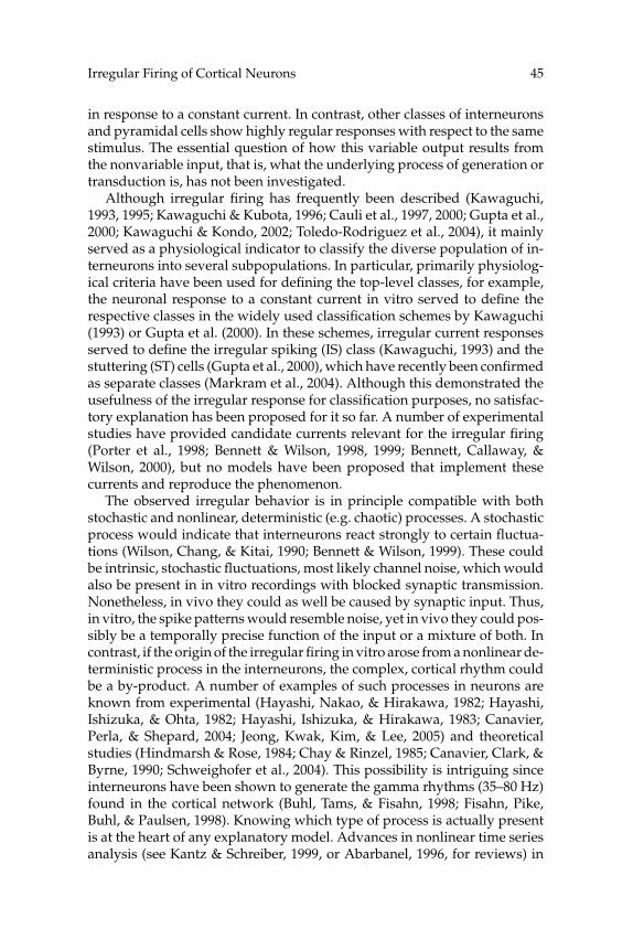
Sample voltage traces for IS and ST cells are shown in Figure 1A andcorresponding ISI series and histograms in Figures 1B and 1C, respectively.IS and ST behaviors were easily discernible on the basis of the ISI histogramshapes, where IS cells showed a moderate peak at the lowest ISIs, directlyfollowed by an exponentially decreasing distribution of ISIs. ST cells exhib-ited a dominant peak around the lowest ISIs, followed by a broad, unimodaldistribution at larger ISIs around the mean interburst interval. The CV (seeFigure 1D) for ST cells was significantly higher (p < 0.005 (n = 4), usingtwo group t-tests) than for IS cells. CVs of these groups were significantlyhigher (ST (n = 4): p < 0.001; IS (n = 4): p < 0.04) than for regular and fast-spiking cells (n = 3). The burst index (BI; percentage of ISIs shorter thantwo times the minimal ISI) for ST cells was significantly higher (p < 0.004,n = 4) than for IS cells (see Figure 1E). These spike statistics persisted over


Figure 1: Raw voltage and ISI data and global statistics for both irregular celltypes. (A) Sample traces for typical IS (A1, c0314) and ST (A2, c0625) cells.(B) Small part (<20%) of the ISI sequences corresponding to the IS (B1) and ST(B2) cell shown in A. (C) ISI histograms for spike trains of the IS (C1) and ST (C2)cell in A(>1000 spikes each). (D) CVs of the three cell types recorded. Diamondsshow averages for a number of recordings from each cell. The star indicates theaverage over the cells in this class. Although CVs vary in each group, the burstsin ST cells lead to distinctively higher CVs 1.5–3. (E) Burst indices for IS and STcell types. Diamonds show averages for a number of recordings from each cell.The filled circle indicates the average over the cells in this class. Note that theBI is mainly useful for distinguishing IS and ST cells, whereas regular spikingcells would have BIs almost equal to 1. Error bars in D and E indicate two SEMaround the mean.

a range of different input currents, where the exact amplitudes dependedon the individual cell (data not shown; see also Markram et al., 2004).

From the subthreshold voltage traces and many other experiments, it isclear that neurons are noisy systems. Note, however, that this does not nec-essarily imply that the high variability of the ISIs is a direct consequence ofthis noise (especially the ST pattern would require additional explanation).One could imagine an intrinsic, deterministic process that interacts onlywith the membrane potential Vm after passing some threshold, analogousto the rapid activation of Na-channels, directly causing a spike. Distinguish-ing between these possibilities is the aim of the following sections.


3.2 Construction of Surrogate and Benchmark Data. The ISI series canbe used to reconstruct the underlying dynamics (Sauer, 1994) or at leastpartially predict the ISI series (Racicot & Longtin, 1997), even when thedynamics are chaotic. The main challenge in the context of patch-clamprecordings is the limited number of spikes (≈10,000 met all the criteria; seesection 3.3) and thus the need to validate the analysis using custom sur-rogate data. Surrogate data share certain properties with the original dataset (e.g., distribution or power spectrum) but with a systematic variationof the property under investigation. We used three types of surrogate data(Theiler et al., 1992):

1. To test for any deterministic features in a time series, we created sur-rogate data from the original ISI data by shuffling the ISIs, denoted asrandomly shuffled (RS) surrogates. This procedure retains all statisti-cal properties that do not depend on the temporal sequence (e.g., char-acteristic statistical properties like mean, variance, and distribution).

2. To test for nonlinear features in a time series, we created surrogatedata from the original data that retain their linear properties; that is,an amplitude-scaled, stationary, linear process is the null hypothesis.These iterative amplitude adjusted Fourier transform (IAAFT)surrogates (Hegger et al., 1999; Schreiber & Schmitz, 2000) weregenerated using the TISEAN routine “surrogates.” IAAFT surrogateswere employed only if any deterministic structure had been detectedwith the first set of surrogate data.

3. To test our data analysis routines on time series generated by a modelwith known nonlinear, deterministic dynamics, we used voltagetraces and ISI series generated by a neuronal model (Hindmarsh& Rose, 1984). The Hindmarsh and Rose (HR) neuron model isgoverned by the equations:

dV(t)dt

= y + 3V2 − V3 − z − I

dy(t)dt

= 1 + 5V2 − y

dz(t)dt

=−r (z − 4(V + 1.6)).

The parameters used for obtaining the chaotic regime were r = 0.006and I ∈ [3.01, 3.08]. For each of these values, noisy versions were sim-ulated, where white gaussian noise was added to I . The standard de-viation of this current noise was adjusted to match the experimentallymeasured subthreshold standard deviation in voltage σ (V) relative tothe total range of values, that is, the spike height. For recorded cells,σ (V)/hspike≈0.5 mV/50 mV = 1%. Three levels of noise, leading to0%, 1%, and 2% subthreshold noise, were simulated in the HR model.


If the time-series analysis algorithms are unable to detect the presenceof determinism in time series generated by this noisy model, they cannotbe expected to successfully detect determinism in the experimental datasets. Since the statistics of the HR data set and the experimental data do notmatch in all respects, we included results for both RS and IAAFT surrogatesfor the HR data.

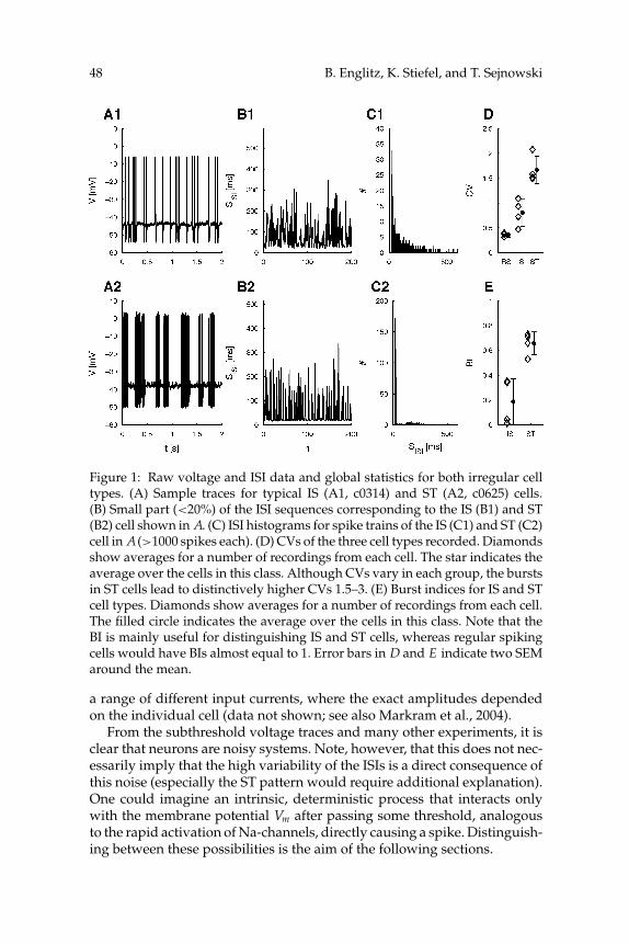
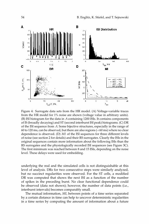
The HR model was chosen since it can deterministically generate highlyirregular ISI sequences in response to constant input, which are reminiscentof the ST pattern (see Figure 4). Although the HR’s ISI distribution capturessome aspects of the ISI distributions—both IS and STcells—this confluenceon the level of the ISI distributions is unlikely to render the model moreeasily predictable on a dynamical level; for example, Racicot and Longtin(1997) conclude that for high enough firing rates, ISI histogram shapes dif-ferent from the original shape can nonetheless lead to good reconstructions.Consequently, other deterministic models could well have the same ISI his-togram as either IS or ST cells and still show the same level of predictabilityas the HR data.

Comparison with surrogate data can be turned into a significance test(Kantz & Schreiber, 1999). To attain a desired significance level p, one drawsN = 1/p samples from the surrogate distribution. Then a quantity of inter-est computed from the given data set is statistically different from thisdistribution with probability p if its value lies below or above all N valuescomputed from the surrogates. Since we chose p = 0.05, 20 surrogates ofeach kind were created and analyzed.

Note that the surrogate data sets were designed to contain the samenumber of spikes as the data sets under investigation. By keeping thisnumber constant, we can view the results of the algorithms modulo theirdependence on the number of data points, that is, if the algorithms candetect determinism in the ISI series generated by the HR model based ononly 1000 spikes but fail to do so in the experimental data, then the sourceof variability in the neuron should have greater complexity. Clearly thisapproach is incomplete in the sense that ISI series from higher-dimensionaldynamics would not be detected, but it can at least provide a weak lowerlimit.

3.3 Stationarity. ISI series SISI were considered stationary or non-stationary based on the standard criterion of weak stationarity (Kantz &Schreiber, 1999), that is, constant mean and standard deviation (SD) overthe recording period. Additionally, we compared the spectral content ofthe first and second half of each recording. To assess the first criterion, thestandard error of the mean (SEM),

SEM(SI SI ) =√∑N

n=1(SI SI (n) − 〈SI SI 〉)2)√(N − 1)N

= sd(SI SI )√N

,


and the standard error of the standard deviation,

SES(SI SI ) =√∑N

n=1(|SI SI (n) − 〈SI SI 〉| − sd(SI SI ))2)√

N= sd(sd(SI SI ))√

N,

were computed for stretches of N = 100 consecutive ISIs. If the distancebetween the running mean and the global mean stayed below 2 SEM (= 95%confidence interval), the null hypothesis of constant mean was maintained,analogously for the SD (not shown). Data were trimmed or excluded entirelyif they failed to match either the mean or SD constancy.

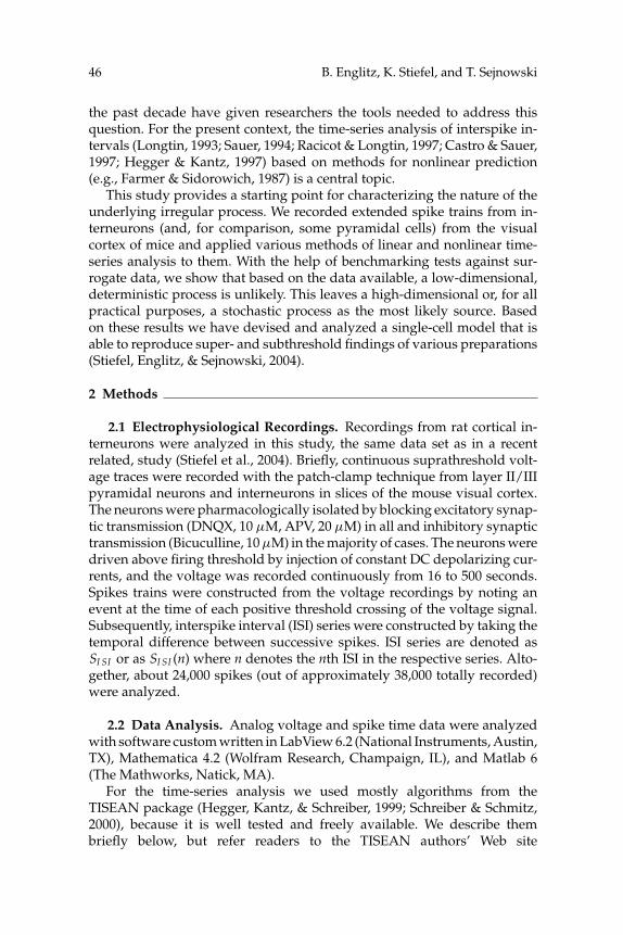
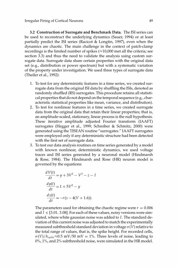
Figure 2B shows the mean, the SD, and the respective running quantitiesfor the four typical ISI sequences from two IS cells (1,2) and two ST (3,4)cells shown in the respective plots of Figure 2A. Overall, 14 of 26 recordings(containing more than 500 spikes each) from five (two IS, three ST) cells(totaling 10,205 spikes) fulfilled weak stationarity and were used in the fol-lowing analyses. In 12 of the 14 recordings, bicuculline and DNQX wereboth applied; in the remaining two recordings, only DNQX was applied.Power spectra were computed using the Matlab function spectrum, whichuses Welch’s averaged periodogram method. As shown in Figure 2C, thespectra of the first (circles) and second (triangles) half of each data set agreewith each other for almost all frequencies. Results for the other weakly sta-tionary time series were comparable. Assessing strong stationarity requiresquantitative comparison of the empirically determined probability transi-tion matrices (Kantz & Schreiber, 1999). Due to the limited number of data,this type of analysis did not yield conclusive results (data not shown).

Figure 2D shows the autocorrelation of the respective ISI sequences(black) and the average (dark gray) surrounding the envelope of 20 RSsurrogates (light gray). For one of the IS cell data (1/2) and all of the STcell (3/3) data, there exists a small yet significant negative correlation (withrespect to the average at higher separations) for one or two steps. Due tothe duality between autocorrelation and power spectrum, this explains thedepression at low frequencies for Figures 2C2 to 2C4.

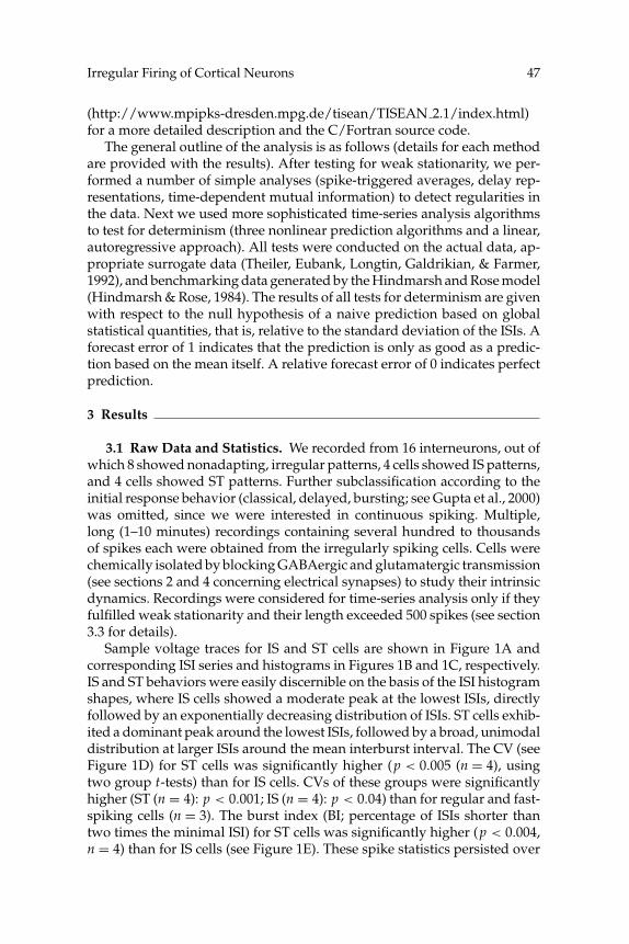
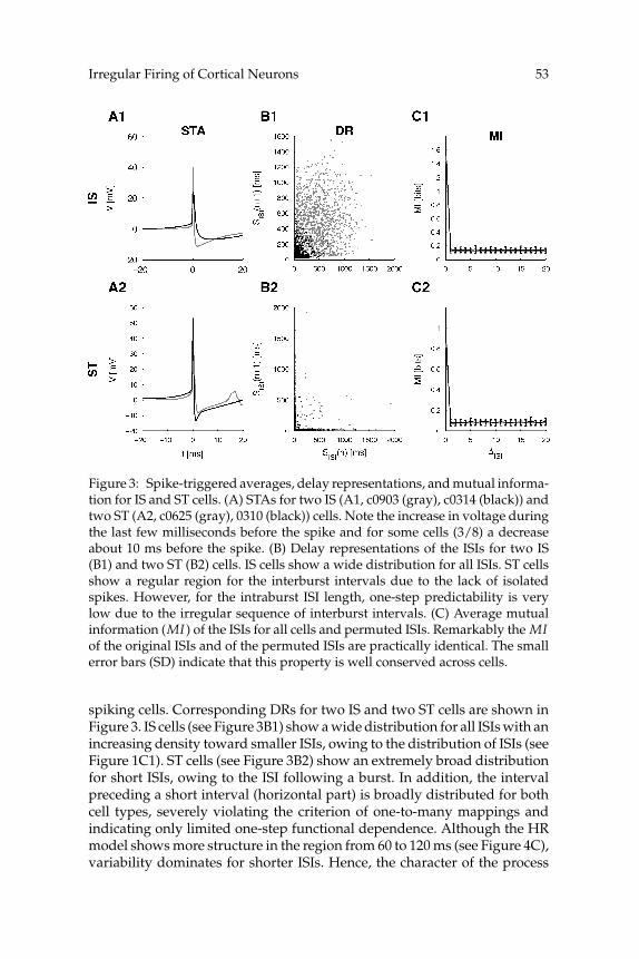
3.4 Spike-Triggered Averages, Delay Representations, and Mutual In-formation. We computed spike-triggered averages (STAs) for isolated andfirst-in-a-burst spikes to detect characteristic voltage kernels in the prespikephase. As shown in Figure 3A, for most cells, the prespike phase wason average flat, with the exception of an increase in voltage in the lastfew milliseconds before the spike. In addition some cells (3/8) showed aslight hyperpolarization about 10 ms before the spike. This type of kernel isalso obtained in cortical neurons responding to a noisy current (Mainen &Sejnowski, 1995). For each cell class, STAs of two typical cells are shown,where base voltages were normalized for easier comparison.


Figure 2: Weak stationarity can be assumed for most ISI sequences. (A) Thesequence of ISIs for typical recordings from the cells (A1) c0314, (A2) c0903,(A3) c0310, and (A4) c0625. (B) The running mean (triangles, solid) and SD(circles, dashed) (points represent averages over 100 consecutive samples) aregraphed, where the error bars indicate their respective standard errors. Thehorizontal lines show the global mean (solid) and SD (dashed), respectively,for visual comparison. (C) Compares the frequency content of the first (circles,solid) and second (triangles, dotted) half of each data set. (D) The autocorrelation(normalized to the correlation for 0 shift) of the original time series (black) andthe mean (dark gray) surrounded by the envelope (light gray) of 20 shuffledsurrogates.

Delay representations (DR), often termed “ISI return maps,” are a simpleyet effective way to identify deterministic mapping rules within a timeseries. A DR is created by simply mapping the nth versus the n + 1th datapoint. If the time series depends on only the last step, the resulting 2D plotshould resemble a functional graph; one-to-many mappings should notoccur. This graph can be disturbed by various sources of noise, which wouldlead to a fuzzy mapping—for the nth data point, a limited distribution ofn + 1th data points occurs. But the influence of noise is not expected tobroaden the distribution of n + 1th data points for a given nth data pointto a flat distribution over the whole range of possible values, which wouldcorrespond to a total loss of predictability. This method can be extended toa greater number of previous steps. We applied this method to all irregular


Figure 3: Spike-triggered averages, delay representations, and mutual informa-tion for IS and ST cells. (A) STAs for two IS (A1, c0903 (gray), c0314 (black)) andtwo ST (A2, c0625 (gray), 0310 (black)) cells. Note the increase in voltage duringthe last few milliseconds before the spike and for some cells (3/8) a decreaseabout 10 ms before the spike. (B) Delay representations of the ISIs for two IS(B1) and two ST (B2) cells. IS cells show a wide distribution for all ISIs. ST cellsshow a regular region for the interburst intervals due to the lack of isolatedspikes. However, for the intraburst ISI length, one-step predictability is verylow due to the irregular sequence of interburst intervals. (C) Average mutualinformation (MI ) of the ISIs for all cells and permuted ISIs. Remarkably the MIof the original ISIs and of the permuted ISIs are practically identical. The smallerror bars (SD) indicate that this property is well conserved across cells.

spiking cells. Corresponding DRs for two IS and two ST cells are shown inFigure 3. IS cells (see Figure 3B1) show a wide distribution for all ISIs with anincreasing density toward smaller ISIs, owing to the distribution of ISIs (seeFigure 1C1). ST cells (see Figure 3B2) show an extremely broad distributionfor short ISIs, owing to the ISI following a burst. In addition, the intervalpreceding a short interval (horizontal part) is broadly distributed for bothcell types, severely violating the criterion of one-to-many mappings andindicating only limited one-step functional dependence. Although the HRmodel shows more structure in the region from 60 to 120 ms (see Figure 4C),variability dominates for shorter ISIs. Hence, the character of the process


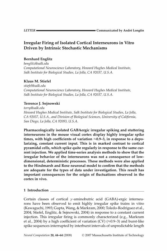
Figure 4: Surrogate data sets from the HR model. (A) Voltage-variable tracesfrom the HR model for 1% noise are shown (voltage value in arbitrary units).(B) ISI histogram for the data in A containing 1200 ISIs. It contains componentsof IS (broadly decaying) and ST (second interburst ISI peak) histograms. (C) DRof the ISI sequence from A. Some bijective structures, especially in the range of60 to 120 ms, can be observed, but there are also regions (<60 ms) where no cleardependence is observed. (D) MI of the ISI sequences for three different levelsof noise (see section 2 for details) and their RS surrogates. Clearly the ISIs in theoriginal sequences contain more information about the following ISIs than theRS surrogates and the physiologically recorded ISI sequences (see Figure 3C).The first minimum was reached between 8 and 15 ISIs, depending on the noiselevel. These delays were used for embedding.

underlying the real and the simulated cells is not distinguishable at thislevel of analysis. DRs for two consecutive steps were similarly analyzed,but no succinct regularities were observed. For the ST cells, a modifiedDR was computed that shows the next ISI as a function of the numberof spikes in the preceding burst. No clear functional dependence couldbe observed (data not shown); however, the number of data points (i.e.,interburst intervals) becomes comparably small.

The mutual information, MI, between points of a time series separatedby a certain distance in time can help to uncover deterministic regularitiesin a time series by computing the amount of information about a future


data point contained at a current point (Abarbanel, 1996). Adapted for ISIseries, the mutual information at a distance of k ISIs is defined as

MI (k) =∑

SI SI (n),SI SI (n+k)

P(SI SI (n), SI SI (n + k)) log2

(P(SI SI (n), SI SI (n + k))

P(SI SI (n))P(SI SI (n + k))

).

The MI of the individual ISI series from both cell types and their respectiveRS surrogates were practically indistinguishable. In Figure 3 the MI for ISIseries and their RS surrogates are shown as averages over the cells for bothIS and ST cells. The vanishingly small error bars indicate that this reflectsthe MI on the level of the individual cells. Based on the surrogate statisticsdescribed above, this means that with respect to the mutual information,neither of the ISI series differed from their permuted counterparts. Theseresults contrast with the MI of the HR model and its RS surrogates, wherea clear difference was observed (see Figure 4D). Hence, at the level ofthe mutual information, the irregular patterns can be distinguished fromthe deterministic HR model, even when the latter includes additive whitenoise. The MI is superior to the autocorrelation function since it is sensitiveto linear and nonlinear correlations (Abarbanel, 1996).

3.5 Linear and Nonlinear Prediction. In order to assess the presenceof determinism in the time series, we applied four different time-seriesprediction methods on each of the data sets and compared their predictionerrors. Three of the methods—the local linear (Farmer & Sidorowich, 1987;Longtin, 1993), simple nonlinear, and the radial basis function methods—rely on a prior embedding of the time series in a reconstructed phase space.An embedding of an ISI series SI SI turns it into a trajectory in D-dimensionalspace by assigning data points SI SI (t), SI SI (t + k), SI SI (t + 2k), . . . , SI SI (t +(D − 1)k) of the time series to the coordinates in the 1st, 2nd, . . . , Dthdimension of a new D-dimensional time series SD

I SI . The first step of thisprocedure is to select a suitable embedding delay, k, and an embeddingdimension, D. Briefly, the local linear method (TISEAN onestep) uses alinear approximation based on neighbors of the current point and theirsuccessors to predict the following point within the phase space. The simplenonlinear prediction method (TISEAN zeroth) computes an average overthe successors of points in a neighborhood of the current point to predict thenext point by taking the mean of all the neighbors’ successors. The radialbasis function method (TISEAN rbf) is a global nonlinear method that fitsthe coefficients of localized basis functions to the reconstructed dynamicsand uses the linear combination of these to predict the next point in thereconstructed phase space. (See Kantz & Schreiber, 1999, for more detaileddescriptions.)

Finally, we used standard autoregressive models (TISEAN ar-model) ofvarious orders in which a weighted, linear sum of previous data points


predicts the next point. No phase space embedding is required in this case.Note that the weights are optimized globally; hence, that is the same rela-tionship, the same weights, holds for the whole time series.

In order to determine k of each ISI series, we selected the first discernibleminimum of the mutual information as a function of the number of ISIs(see Figure 3C; Abarbanel, 1996). For the recorded ISI series and all the RSsurrogates, this minimum lay between 1 and 4 ISIs. The first zero crossingof the autocorrelation always yielded k = 1 ISI (see Figure 2D). In contrastk’s between 9 and 15 ISIs (depending on the noise level) were found for theHR neuron (see Figure 4D). As expected, the mutual information degradedfaster for stronger noise amplitudes. Averages over the given ranges of k’swere used in the following to reduce the bias of an inappropriate choiceof k. From the original work of Takens (1981), the reconstruction shouldbe stable under (small) variations of k. The positions of the minima werelargely independent of the number of boxes used in estimating the mu-tual information. No significant increases of the mutual information wereobserved for k’s beyond the range shown.

The appropriate D for the embedding is often chosen by the false nearest-neighbor method (FNN; Kennel, Brown, & Abarbanel, 1992). We appliedthis method to all time series using the range of k’s found. Although sig-nificant quantitative differences were seen, none of the time series, exceptfor the noise-free HR model, fulfilled the criterion of dropping below 1%to 5% of false nearest neighbors. Using low plateaus (<20% FNNs; Kennelet al. 1992) as a criterion for the correct embedding dimension under theinfluence of noise, the noisy HR models embedded in dimensions 4 to 6.The recorded ISI series did not reach lower plateaus (≈40% FNNs) thantheir RS surrogates, which can taken as an indication that no further de-terministic dynamics were separated by increasing D. A marked differencewas already apparent at D = 1: the clean HR data started at only 50% FNNs,whereas the recorded ISIs started at about 98% FNNs.

Since we were not able to confidently determine Ds for most of thedata sets, we performed the tests for determinism with a range of relevantDs. Figure 5 shows the results for all data sets and all algorithms. Allaverage forecast errors are given with respect to the standard deviationof the respective ISI series. A relative forecast error of 1 corresponds totrivially guessing the mean every time. To avoid overloading the graphswith curves, only the error bars, rather than individual predictions for eachrecord and embedding delay, are shown. These averages and the error barswere computed over the individual recordings and the relevant range of k(see above).

Both the phase-space prediction methods (local linear, see Figure 5A; 0thorder, see Figure 5B; radial basis function, see Figure 5C) and the linearmethod (autoregressive model, see Figure 5D) detected determinism in theHR ISI series. Of the nonlinear methods, the local linear method performedbest and showed the shallowest dependence on the embedding dimension.


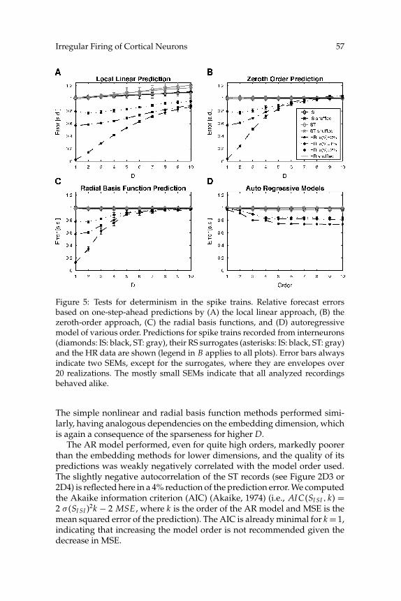
Figure 5: Tests for determinism in the spike trains. Relative forecast errorsbased on one-step-ahead predictions by (A) the local linear approach, (B) thezeroth-order approach, (C) the radial basis functions, and (D) autoregressivemodel of various order. Predictions for spike trains recorded from interneurons(diamonds: IS: black, ST: gray), their RS surrogates (asterisks: IS: black, ST: gray)and the HR data are shown (legend in B applies to all plots). Error bars alwaysindicate two SEMs, except for the surrogates, where they are envelopes over20 realizations. The mostly small SEMs indicate that all analyzed recordingsbehaved alike.

The simple nonlinear and radial basis function methods performed simi-larly, having analogous dependencies on the embedding dimension, whichis again a consequence of the sparseness for higher D.

The AR model performed, even for quite high orders, markedly poorerthan the embedding methods for lower dimensions, and the quality of itspredictions was weakly negatively correlated with the model order used.The slightly negative autocorrelation of the ST records (see Figure 2D3 or2D4) is reflected here in a 4% reduction of the prediction error. We computedthe Akaike information criterion (AIC) (Akaike, 1974) (i.e., AI C(SI SI , k) =2 σ (SI SI )2k − 2 MSE , where k is the order of the AR model and MSE is themean squared error of the prediction). The AIC is already minimal for k = 1,indicating that increasing the model order is not recommended given thedecrease in MSE.


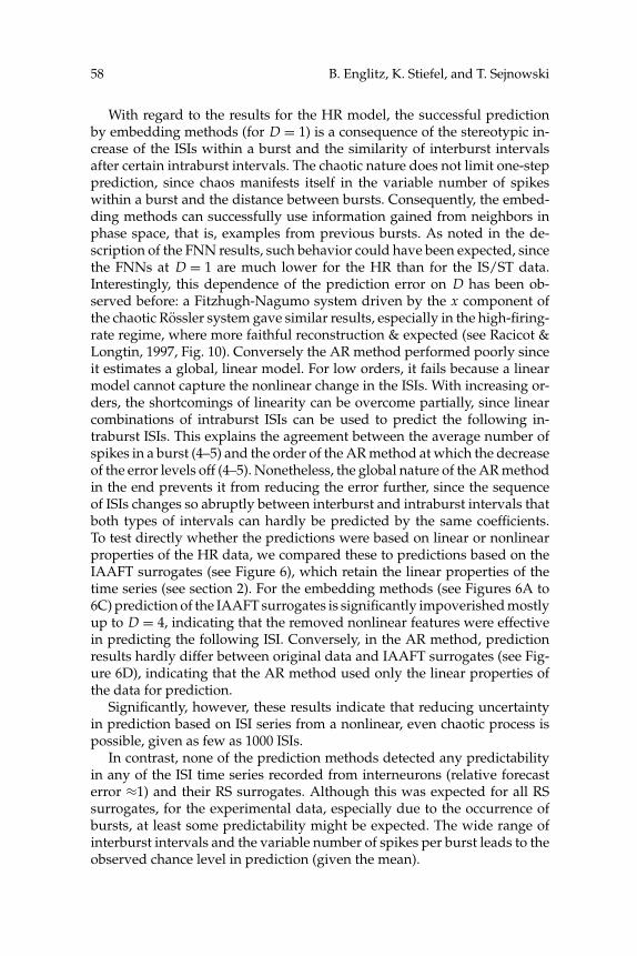
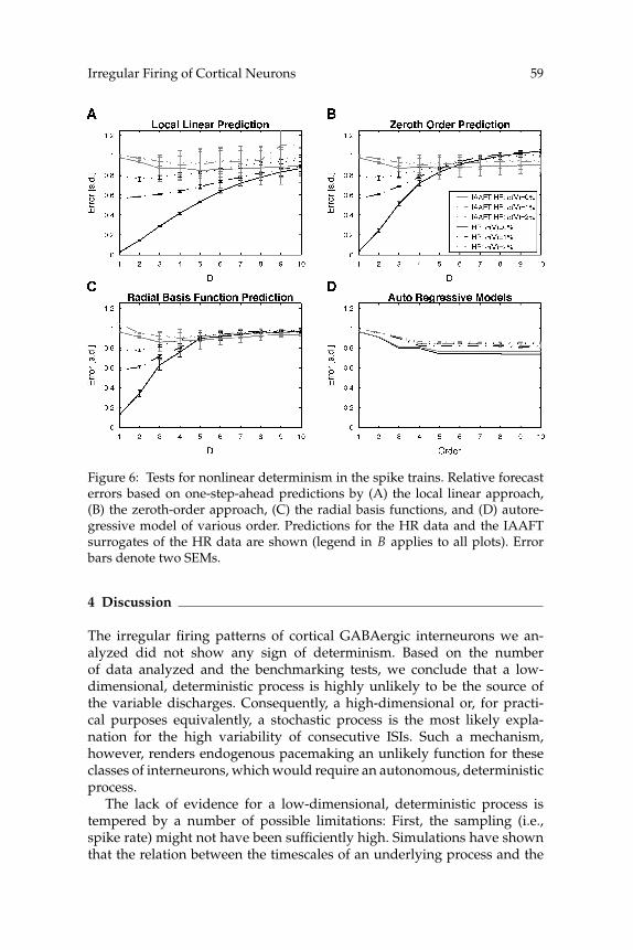
With regard to the results for the HR model, the successful predictionby embedding methods (for D = 1) is a consequence of the stereotypic in-crease of the ISIs within a burst and the similarity of interburst intervalsafter certain intraburst intervals. The chaotic nature does not limit one-stepprediction, since chaos manifests itself in the variable number of spikeswithin a burst and the distance between bursts. Consequently, the embed-ding methods can successfully use information gained from neighbors inphase space, that is, examples from previous bursts. As noted in the de-scription of the FNN results, such behavior could have been expected, sincethe FNNs at D = 1 are much lower for the HR than for the IS/ST data.Interestingly, this dependence of the prediction error on D has been ob-served before: a Fitzhugh-Nagumo system driven by the x component ofthe chaotic Rossler system gave similar results, especially in the high-firing-rate regime, where more faithful reconstruction & expected (see Racicot &Longtin, 1997, Fig. 10). Conversely the AR method performed poorly sinceit estimates a global, linear model. For low orders, it fails because a linearmodel cannot capture the nonlinear change in the ISIs. With increasing or-ders, the shortcomings of linearity can be overcome partially, since linearcombinations of intraburst ISIs can be used to predict the following in-traburst ISIs. This explains the agreement between the average number ofspikes in a burst (4–5) and the order of the AR method at which the decreaseof the error levels off (4–5). Nonetheless, the global nature of the AR methodin the end prevents it from reducing the error further, since the sequenceof ISIs changes so abruptly between interburst and intraburst intervals thatboth types of intervals can hardly be predicted by the same coefficients.To test directly whether the predictions were based on linear or nonlinearproperties of the HR data, we compared these to predictions based on theIAAFT surrogates (see Figure 6), which retain the linear properties of thetime series (see section 2). For the embedding methods (see Figures 6A to6C) prediction of the IAAFT surrogates is significantly impoverished mostlyup to D = 4, indicating that the removed nonlinear features were effectivein predicting the following ISI. Conversely, in the AR method, predictionresults hardly differ between original data and IAAFT surrogates (see Fig-ure 6D), indicating that the AR method used only the linear properties ofthe data for prediction.

Significantly, however, these results indicate that reducing uncertaintyin prediction based on ISI series from a nonlinear, even chaotic process ispossible, given as few as 1000 ISIs.

In contrast, none of the prediction methods detected any predictabilityin any of the ISI time series recorded from interneurons (relative forecasterror ≈1) and their RS surrogates. Although this was expected for all RSsurrogates, for the experimental data, especially due to the occurrence ofbursts, at least some predictability might be expected. The wide range ofinterburst intervals and the variable number of spikes per burst leads to theobserved chance level in prediction (given the mean).


Figure 6: Tests for nonlinear determinism in the spike trains. Relative forecasterrors based on one-step-ahead predictions by (A) the local linear approach,(B) the zeroth-order approach, (C) the radial basis functions, and (D) autore-gressive model of various order. Predictions for the HR data and the IAAFTsurrogates of the HR data are shown (legend in B applies to all plots). Errorbars denote two SEMs.

4 Discussion

The irregular firing patterns of cortical GABAergic interneurons we an-alyzed did not show any sign of determinism. Based on the numberof data analyzed and the benchmarking tests, we conclude that a low-dimensional, deterministic process is highly unlikely to be the source ofthe variable discharges. Consequently, a high-dimensional or, for practi-cal purposes equivalently, a stochastic process is the most likely expla-nation for the high variability of consecutive ISIs. Such a mechanism,however, renders endogenous pacemaking an unlikely function for theseclasses of interneurons, which would require an autonomous, deterministicprocess.

The lack of evidence for a low-dimensional, deterministic process istempered by a number of possible limitations: First, the sampling (i.e.,spike rate) might not have been sufficiently high. Simulations have shownthat the relation between the timescales of an underlying process and the


rate at which the underlying process is sampled is a critical determinantfor successful reconstruction of the original system dynamics (Racicot &Longtin, 1997). Higher sampling rates typically lead to better quality of re-construction, although lower rates also resulted in a considerable reductionin prediction error. Whether the sampling rate, that is, the mean firing rate,was adequate for the (potentially) underlying timescales cannot be knownunless prediction is (at least partially) achieved.

A second possible limitation for the lack of evidence of determinismcould be the existence of a large, slow noise source. If some noise sourceexists, which influences the dynamics rarely but severely, the potentiallydetectable determinism would be seriously disturbed. The footprints of thissource could be hidden at certain spike onsets and thus remain undetectedin the STA.

A final, and probably the most important, limitation of our analysis isthat neither the number of spike trains nor the number of spikes is ad-equate to reach precise conclusions. Unfortunately, obtaining longer, sta-tionary data has proven to be extremely difficult due to the fragile natureof interneurons under the required recording conditions (extended stimu-lation and penetration). In this context, patch clamp recordings had to bepreferred over extracellular recordings in order to stimulate the (otherwisesilent) cells and check for isolation. We attempted to compensate the lowspike counts by the use of appropriate surrogate data and selecting thelongest and most stationary spike trains only. Thus, although it is difficultto reach precise conclusions, the complete lack of predictability for the ex-perimental data is indicative of the lack of a low-dimensional, deterministicprocess. At the same time, it should be emphasized that the rapid decline ofpredictability with increasing D for the HR data indicates that for higher di-mensions, the number of spikes is too low to distinguish determinism fromrandomness.

In the case of a stochastic process, it remains to be explained why thedistribution of the ISIs does not resemble the distribution of the underlyingnoise sources; neither follows a Poisson or a gamma distribution. A specificmechanism needs to exist that transforms the distribution of the underlyingprocess into the observed distribution. It is known that this cell class exhibitsa high responsiveness with respect to certain weak inputs (Wilson et al.,1990), that is, some input fluctuations are gated into eliciting spikes or evenburst sequences.

A plausible general candidate mechanism would be a subcritical Hopfbifurcation, that is, stochastic switching between a stable fixed point (restingpotential) and a stable limit cycle (repetitive spiking) as detailed in Ermen-trout (1998) and Brown, Feerick, and Feng (2001). This mechanism and thereported results are incorporated in our recently proposed model (Stiefel,Englitz, & Sejnowski, 2007) which details how interneurons could trans-form voltage noise into irregular spike times. This Hodgkin-Huxley typemodel (Hodgkin & Huxley, 1952) includes a fast K +-conductance, which


creates a substantial region of bistability in phase space (switching region;Rowat, 2007) between the rest state and continuous spiking. Noise caneasily transfer the neuron between these modes, thus exhibiting stochasticswitching between burst firing, single spikes, and quiescence. For differentparameter ranges, the model resembles the IS and the ST behavior in termsof CV and also ISI distribution.

The observed variability could also arise as a superposition of manydeterministic processes, especially electrically coupled interneurons. Thiswould mean that the observed variability would derive from network ac-tivity rather than single-neuron dynamics. We did not use pharmacologicalblockers of gap junctions as they show limited specificity and thus alsointerfere with other intracellular mechanisms and are therefore inadequatefor studying endogenous dynamics (Rozental, Srinivas, & Spray, 2001).Several factors speak against a contribution of gap junctions to our data.First, we did not observe any potentials that could have originated in otherneurons (spikelets) in any of our recordings. This was true for both near-threshold potentials (used for the time series analysis) and recordings athyperpolarized potentials. The later recording conditions make a detectionof gap-junction-mediated potentials much more likely due to the voltagedifference between coupled cells and the quiescence of the membrane po-tential. Second, gap junctions mostly couple interneurons of the same class(Amitai et al., 2002). Because all recorded cells were not spontaneously ac-tive, other coupled cells are unlikely to be spontaneously active. Thus, wecan be reasonably sure of the absence of gap-junction-mediated potentialsin our recordings.

The main source of noise in isolated neurons is channel noise, generatedby the stochastic opening and closing of individual ion channels (Hille,2001). The existence of irregular activity is indicative of a high sensitivity tonoise and fluctuations, which becomes functionally important in vivo whenmassive barrages of synaptic potentials arrive at the dendrite (Destexhe,Rudolph, & Par, 2003). Interneurons should be strongly driven by this highlyirregular input and may introduce additional variability. This sensitivity ofthe spike initiation dynamics of ST and IS interneurons to voltage noiseis thus likely to preserve or even enhance the discharge variability of allneurons in the cortical network.

Acknowledgments

We thank Lee Campbell for providing data acquisition software,the Deutsche Forschungsgemeinschaft (K.M.S.), the Studienstiftung desdeutschen Volkes (B.E.), the Fulbright Commission (B.E.), and the HowardHughes Medical Institute (T.J.S.) for financial support and EckehardOlbrich, Jean-Marc Fellous, Peter J. Thomas, Jurgen Jost, Charles Stevens,and Nils Bertschinger for helpful discussions. Further, we thank the twoanonymous reviewers for their helpful comments.


References

Abarbanel, H. (1996). Analysis of observed chaotic data. Berlin: Springer.Akaike, H. (1974). A new look at the statistical model identification. IEEE Transactions

on Automatic Control, 19, 716–723.Amitai, Y., Gibson, J. R., Beierlein, M., Patrick, S. L., Ho, A. M., Connors, B. W., &

Golomb, D. (2002). The spatial dimensions of electrically coupled networks ofinterneurons in the neocortex. J. Neurosci., 22(10), 4142–4152.

Bennett, B., Callaway, J., & Wilson, C. (2000). Intrinsic membrane properties under-lying spontaneous tonic firing in neostriatal cholinergic interneurons. J. Neurosci.,20(22), 8493–8503.

Bennett, B., & Wilson, C. (1998). Synaptic regulation of action potential timing inneostriatal cholinergic interneurons. J. Neurosci., 18(20), 8539–8549.

Bennett, B., & Wilson, C. (1999). Spontaneous activity of neostriatal cholinergic in-terneurons in vitro. J. Neurosci., 19(13), 5586–5596.

Brown, D., Feerick, S., & Feng, J. (2001). Significance of random neuronal drive.Neurocomputing, 38–40, 111–119.

Buhl, E., Tams, G., & Fisahn, A. (1998). Cholinergic activation and tonic excitationinduce persistent gamma oscillations in mouse somatosensory cortex in vitro. J.Physiol., 513(Pt. 1), 117–126.

Canavier, C., Clark, J., & Byrne, J. (1990). Routes to chaos in a model of a burstingneuron. Biophys. J., 57(6), 1245–1251.

Canavier, C. C., Perla, S. R., & Shepard, P. D. (2004). Scaling of prediction errordoes not confirm chaotic dynamics underlying irregular firing using interspikeintervals from midbrain dopamine neurons. Neuroscience, 129(2), 491–502.

Castro, R., & Sauer, T. (1997). Correlation dimension of attractors through interspikeintervals. Physical Review E, 55, 287–290.

Cauli, B., Audinat, E., Lambolez, B., Angulo, M. C., Ropert, N., Tsuzuki, K., Hestrin,S., & Rossier, J. (1997). Molecular and physiological diversity of cortical nonpyra-midal cells. J. Neurosci., 17(10), 3894–3906.

Cauli, B., Porter, J. T., Tsuzuki, K., Lambolez, B., Rossier, J., Quenet, B., & Audinat, E.(2000). Classification of fusiform neocortical interneurons based on unsupervisedclustering. Proc. Natl. Acad. Sci. USA, 97(11), 6144–6149.

Chay, T., & Rinzel, J. (1985). Bursting, beating, and chaos in an excitable membranemodel. Biophys. J., 47(3), 357–366.

Destexhe, A., Rudolph, M., & Par, D. (2003). The high-conductance state of neocor-tical neurons in vivo. Nat. Rev. Neurosci., 4(9), 739–751.

Ermentrout, B. (1998). In C. Koch & I. Segev (Eds.), Methods in neuronal modeling(pp. 93–129). Cambridge, MA: MIT Press.

Farmer, J. D., & Sidorowich, J. (1987). Predicting chaotic time series. Physical ReviewLetters, 59, 845.

Fisahn, A., Pike, F., Buhl, E., & Paulsen, O. (1998). Cholinergic induction of networkoscillations at 40 Hz in the hippocampus in vitro. Nature, 394(6689), 186–189.

Gupta, A., Wang, Y., & Markram, H. (2000). Organizing principles for a diversityof GABAergic interneurons and synapses in the neocortex. Science, 287(5451),273–278.


Hayashi, H., Ishizuka, S., & Hirakawa, K. (1983). Transition to chaos via intermittencyin the onchidium pacemaker neuron. Physics Letters, 98a(8, 9), 435–438.

Hayashi, H., Ishizuka, S., & Ohta, M. (1982). Chaotic behavior in the onchidium giantneuron under sinusoidal stimulation. Physics Letters, 88a(8), 435–438.

Hayashi, H., Nakao, M., & Hirakawa, K. (1982). Chaos in the self-sustained oscillationof an excitable biological membrase under sinusoidal stimulation. Physics Letters,88a(5), 265–266.

Hegger, R., & Kantz, H. (1997). Embedding of sequences of time intervals. Europhys.Lett., 38, 267–272.

Hegger, R., Kantz, H., & Schreiber, T. (1999). Practical implementation of nonlineartime series methods: The TISEAN package. CHAOS, 9, 413–435.

Hille, B. (2001). Ion channels of excitable membranes (3rd ed.). Sunderland, MA: SinauerAssociates.

Hindmarsh, J., & Rose, R. (1984). A model of neuronal bursting using three coupledfirst order differential equations. Proc. R. Soc. Lond. B. Biol. Sci., 221(1222), 87–102.

Hodgkin, A. L., & Huxley, A. F. (1952). A quantitative description of membranecurrent and its application to conduction and excitation in nerve. J. Physiol.,117(4), 500–544.

Jeong, J., Kwak, Y., Kim, Y. I., & Lee, K. J. (2005). Dynamical heterogeneity of suprachi-asmatic nucleus neurons based on regularity and determinism. J. Comput. Neu-rosci., 19(1), 87–98.

Kantz, H., & Schreiber, T. (1999). Nonlinear time series analysis. Cambridge: CambridgeUniversity Press.

Kawaguchi, Y. (1993). Groupings of nonpyramidal and pyramidal cells with specificphysiological and morphological characteristics in rat frontal cortex. J. Neuro-physiol., 69(2), 416–431.

Kawaguchi, Y. (1995). Physiological subgroups of nonpyramidal cells with specificmorphological characteristics in layer II/III of rat frontal cortex. J. Neurosci., 15(4),2638–2655.

Kawaguchi, Y., & Kondo, S. (2002). Parvalbumin, somatostatin and cholecystokininas chemical markers for specific GABAergic interneuron types in the rat frontalcortex. J. Neurocytol., 31(3–5), 277–287.

Kawaguchi, Y., & Kubota, Y. (1996). Physiological and morphological identifica-tion of somatostatin- or vasoactive intestinal polypeptide-containing cells amongGABAergic cell subtypes in rat frontal cortex. J. Neurosci., 16(8), 2701–2715.

Kennel, M. B., Brown, R., & Abarbanel, H. D. I. (1992). Determining minimumembedding dimension using a geometrical construction. Physical Review A, 45,3403–3411.

Longtin, A. (1993). Nonlinear forecasting of spike trains from sensory neurons.International Journal of Bifurcation and Chaos, 3, 651–661.

Mainen, Z., & Sejnowski, T. (1995). Reliability of spike timing in neocortical neurons.Science, 268(5216), 1503–1506.

Markram, H., Toledo-Rodriguez, M., Wang, Y., Gupta, A., Silberberg, G., & Wu, C.(2004). Interneurons of the neocortical inhibitory system. Nat. Rev. Neurosci., 5(10),793–807.


Porter, J. T., Cauli, B., Staiger, J. F., Lambolez, B., Rossier, J., & Audinat, E. (1998).Properties of bipolar VIPergic interneurons and their excitation by pyramidalneurons in the rat neocortex. Eur. J. Neurosci., 10(12), 3617–3628.

Racicot, D. M., & Longtin, A. (1997). Interspike interval attractors from chaoticallydriven neuron models. Physica D, 104, 184–204.

Rowat, P. (2007). Interspike interval statistics in the stochastic Hodgkin-Huxleymodel: Coexistence of gamma frequency bursts and highly irregular firing. NeuralComput., 19(5), 1215–1250.

Rozental, R., Srinivas, M., & Spray, D. (2001). How to close a gap junction channel:Efficacies and potencies of uncoupling agents. Methods Mol. Biol., 154, 447–476.

Sauer, T. (1994). Reconstruction of dynamical systems from interspike intervals.Physical Review Letters, 72(24), 3811–3814.

Schreiber, T., & Schmitz, A. (2000). Surrogate time series. Physica D, 142, 346.Schweighofer, N., Doya, K., Fukai, H., Chiron, J. V., Furukawa, T., & Kawato, M.

(2004). Chaos may enhance information transmission in the inferior olive. Proc.Natl. Acad. Sci. USA, 101(13), 4655–4660.

Stiefel, K., Englitz, B., & Sejnowski, T. (2004). Irregular firing of cortical interneurons.Paper presented at the 34th Annual Meeting of the Society for NeuroscienceAbstracts, San Diego, CA.

Stiefel, K., Englitz, B., & Sejnowski, T. (2007). The irregular firing of cortical interneuronsin vitro is due to fast K+-current kinetics. Manuscript submitted for publication.

Takens, F. (1981). Detecting strange attractors in turbulence. In D. A. Rand & L.-S.Young (Eds.), Dynamical systems and turbulence (vol. 898, p. 366). Berlin: Springer.

Theiler, J., Eubank, S., Longtin, A., Galdrikian, B., & Farmer, J. D. (1992). Testing fornonlinearity in time series: The method of surrogate data. Physica D, 58, 77–94.

Toledo-Rodriguez, M., Blumenfeld, B., Wu, C., Luo, J., Attali, B., Goodman, P., &Markram, H. (2004). Correlation maps allow neuronal electrical properties to bepredicted from single-cell gene expression profiles in rat neocortex. Cereb. Cortex,14, 1310–1327.

Wilson, C., Chang, H., & Kitai, S. (1990). Firing patterns and synaptic potentialsof identified giant aspiny interneurons in the rat neostriatum. J. Neurosci., 10(2),508–519.

Received August 16, 2006; accepted April 3, 2007.

Documents

Irregular Firing of Isolated Cortical Interneurons - CNL Publications