Embed Size (px)
Citation preview

1
Chapter 1
Introduction
In this chapter, motivation for the dissertation is first introduced in Section 1.1. A
brief review of the related researches is presented in Section 1.2. Section 1.3 gives an
overview of the dissertation. Finally, the organization of the dissertation is stated in
Section 1.4.
1.1 Motivation
Polynomial-style sharing (PSS) [1] and visual cryptography (VC) [2] are two
well-known sharing approaches to secure an image file for storage and transmission.
In general, the two approaches share a secret or important image among several
extremely noise-like images called shadows (or shares). Combing these shadows can
reconstruct the secret or important image later. Several extended researches of [1] and
[2] about image sharing have been reported. Examples include, but not limit to, Wang
and Su‟s reduction of memory cost for shadows [3]; Lin and Tsai‟s extension of
binary VC to grayscale images [4]; Lin and Lin‟s two-in-one sharing method VCPSS
[5] that combined visual cryptography (VC) and polynomial-style sharing (PSS).
Polynomial-style sharing using polynomials [1, 3, 6-9] is one of the popular
secret sharing approaches to protect secret images. This kind of approach can restore
the secret images without any loss, and the size of each shadow image can even be
several times smaller than that of the given secret image [3, 6]. Therefore,
space-wasting is seldom a problem for sharing using polynomials. However, the
retrieval speed is very slow because of the evaluation of polynomials.

2
On the contrary, a fast approach called visual cryptography (VC) [2, 4, 10-12],
which shares a secret image using several “size-enlarged” transparencies, is often
utilized to deal with images whose brightness are only of a few levels (for example,
black-and-white, 3-levels, or 4-levels). In the recovery phase of VC, a “size-enlarged”
version of the secret image can be visually decoded instantly by human eyes after
“physically stacking” the transparencies; therefore, there is no need to use a computer.
However, as the images‟ gray levels increase from 2 or 4 levels to 256 levels, human
eyes can no longer be utilized in decoding by generating transparencies, unless the
256-level image is first pre-quantized to, saying, a 2-level image by approximation
techniques such as halftone. Therefore, the decoding is not error-free, and it is just an
approximation. Nevertheless, if we use a computer to replace the roles of human eyes
as the decoder for VC, then there is no need to use the error-introduced 256-to-2
pre-quantization, for the computer can handle each bit-plane individually.
Unfortunately, even though the concept of using physical transparencies can be
transformed to the concept of using digital files in a computer or network, each digital
file is several times larger than the secret image file itself [13-15], for each
transparency in VC is already several times larger than the secret image.
Although people can use the digitalized version of an elegant method proposed
in [16] that has no size expansion because of using probabilistic skill; the recovered
secret image is not lossless. In general, size expansion problem is a disadvantage for
VC-based fast approaches: to store digital shadow images in the computer often
requires large storage space.
From the analysis in above two paragraphs, we can see that these two kinds of
sharing approaches are quite different, and each has its own speed-vs.-space
advantage and disadvantage. A question arises naturally: “can a sharing system have
both advantages in speed and space?” In other words, can people have some

3
economical-size shadows which can reconstruct the given secret image in a loss-free
manner after only using a few operations to decode each pixel? The answer is positive.
Wang et al. [17-18] had gracefully provided their answer, to certain level, in their
second scheme [18] which is an (n, n) scheme.
In Chapter 2, we will improve Wang et al.‟s (n, n) scheme in order to have the
“missing-allowable” (k, n)-threshold ability, i.e. in the reconstruction of the secret,
any k out of the n shadows will work. The proposed scheme generates the n desired
shadows for a given color (grayscale/binary) image A, so that each shadow‟s size is
less than two times the size of A. Furthermore, the lossless decoding process only uses
quite a few exclusive-OR (XOR) operations. Hence there is no complex computation.
In above two well-known sharing approaches, i.e. PSS [1] and VC [2], there are
some other extensions which are “applications-oriented”, such as (1) user-friendly
shadows [7, 19] for easier management of shadows, and (2) progressive decoding [9,
19-22] of an image which is moderately sensitive but still need to be processed every
day. For example, among the PSS approaches [7, 9, 20], Thien and Lin [7] firstly
introduced the idea of using “user-friendly” (i.e. visually-recognizable) shadows;
Chen and Lin [9] designed a sharing method for progressive transmission of images;
Hung et al. [20] also proposed a progressive sharing method according to three
pre-specified thresholds. In VC approaches [19, 21-22], Jin et al. [21] developed a
progressive VC technique for grayscale/color images with three types of decryptions
to enable the recovery in varying qualities; Fang reported in [19] a progressive
viewing method which extended Fang and Lin‟s work [22] to utilize user-friendly
shadows and progressive decoding simultaneously.
From the viewpoint of shadows‟ management, to classify or locate a shadow,
attaching a name-tag to each shadow in advance is needed if each shadow looks like
random-noise (most reported methods [9, 20-22] have this kinds of shadows). Another

4
way is to use visually-identifiable shadows. They are also called as user-friendly
shadows (first mentioned in Ref. [7], then in Ref. [19]), for their visually-identifiable
feature (each shadow looks like a visual-quality-reduced version of a given image)
makes the managing job of shadows become easier for database manager. For
example, if there are 100 important images and each creates 2 to 17 shadows of its
own. Then it is easy to visually recognize that a stored shadow is from, saying, House
image, rather than from other 99 images.
Both [7] and [19] can be used in a system consisting of distributed storage
branches, and each branch stores one of the shadow images. When a branch needs the
original image, all other branches can transmit its own shadow to the receiver, and all
other branches may transmit simultaneously in parallel. From the viewpoint of a local
manager (the manager of a branch), noise-like shadow images are difficult to identify
and manage, i.e. they are not user-friendly. Therefore, it is more convenient for a local
manager to manage shadow images that look like visual-quality-reduced versions of
the original images. Hence, user-friendly shadows such as those produced by [7] and
[19] are welcome in distributed storage system. On the other hand, to avoid unfaithful
local manager from selling the shadow stored in his branch, it is suggested that the
image quality of each shadow cannot be too good.
Although Thien and Lin [7] firstly introduced the idea of using “user-friendly”
(visually-recognizable) shadows, their method is not progressive, and the
reconstruction by all shadows is not lossless. These two weaknesses will be avoided
by our method proposed in Chapter 3. So far, only Fang‟s method [19] (which is
lossless when all shadows are collected) simultaneously owns the following two
application-convenient features: 1) user-friendly shadows and 2) progressive decoding.
Unfortunately, its shadows are four times larger than the input image; and thus not
economical in memory space if implemented on computers. To improve it, we

5
propose in Chapter 3 a novel progressive and user-friendly approach based on
modulus operations. Better than Fang‟s method [19], our method possesses extra
advantages: 3) non-expansion in size of shadows; 4) controllable quality of shadow
images. Meanwhile, like Fang‟s method, our method has lossless recovery when all n
shadows are used, and the decoding complexity is O(k) for the reconstruction using k
shadows (kn).
In the above, if a secret image is to be protected by some participants in a team,
then each participant can hold some of the generated shadows after sharing the secret
image. Later in a meeting, when the number of collected shadows from participants
reaches a specified threshold value, then the shared secret image is reconstructed.
However, in real life, a project team often process more than one secret image
simultaneously. Therefore, some researches [23-29] shared multiple images in one
encoding process. For example, the elegant PSS scheme [23] presented by Feng et al.
used Lagrange interpolation to deal with multi-secret images. Their method is an
economical method, for it has a very low O/I size ratio between 1 and 2, i.e. total
input images‟ size is at least 50% of the total output shadows‟ size, and 100% is
possible. But the computational complexity O(log2k) would be needed to reconstruct
each secret pixel by using Lagrange interpolation from k required shadows. To the
contrary, to save computational operations in the retrieval of secret images, Visual
Cryptography (VC) schemes can be used. For example, Shyu et al. used two circular
shadows to design a VC scheme [24] which can share more than two secret images.
Feng et al. also presented a multi-secret VC scheme [25], and their shadows are in
rectangular shape. By stacking the shadows (know as transparencies in VC field),
these VC schemes are very fast in revealing all secret images. The disadvantage of
using VC methods is their high O/I size ratio due to the high pixel-expansion-rate
(per≧2) in generating shadows. (As for the disadvantage of the low-contrast of the

6
images recovered by stacking transparencies; it can be avoided if VC methods are
implemented on computer.) When VC methods are implemented on computer to
reconstruct n original secret images error-freely, the complexity to decode a pixel of a
secret image would be O(n) due to the high per. Besides PSS and VC schemes,
Alvarez et al. also developed a multi-secrets sharing scheme [26] for color images
with different sizes based on modulus operations. Albeit their O/I size ratio is a very
good value (n+1)/n after sharing n secret images by n+1 shadows; their reconstruction
in each secret pixel needs one modulus operation and many mathematical operations
(addition or subtraction) whose computational complexity is O(n).
Among the multi-secrets schemes [23-26], no one can simultaneously own the
two advantages: (1) O/I size ratio is 1, and (2) only constant number of operations is
needed to reconstruct each secret pixel. To achieve these two advantages
simultaneously, we propose in Chapter 4 a novel sharing scheme for multiple images,
by using modulus (MOD) and exclusive-OR (XOR) operations. The proposed method
generates n extremely noise-like shadows for n given binary/grayscale/color secret
images (notably, the n given images all have the same size), and each shadow‟s size is
identical to each given image. When the n shadows replace the n original secret
images in image database; since our O/I size ratio is always 1, we will not need extra
storage space. Furthermore, after gathering all n shadows, our lossless decoding
process only uses one XOR, one MOD, one addition (ADD) and one subtraction
(SUB) operations (symbolized as “⊕”, “Mod”, “+” and “-”) to reconstruct each
pixel‟s 8-bits value of each secret image. This holds for all values of n. Hence, no
matter how many secret images are shared, the CPU time in decoding each secret
image will not increase. In summary, the proposed method is not only economical in
storage space of shadows but also fast in decoding.

7
1.2 Related Studies
1.2.1 Image Sharing Schemes with Small Shadows or Fast Decoding
Shamir‟s polynomial secret sharing [1] is a popular technology to protect secret
images. This technology uses polynomials to divide the secret image into several
shadows, which have the same size as the secret image for perfect security. After an
advanced method proposed by Thien and Lin [6] to improve [1], the size of each
shadow image can even be k times smaller than that of the given secret image by
letting k coefficients in the k-1 degree polynomial be the gray values of k pixels. Then,
Wang and Su proposed a better method in [3] to encode the difference image from the
secret image using Huffman coding scheme and evaluate the arithmetic calculations
of the sharing functions in a power-of-two Galois Field GF(2t). Their experiment
results show that each generated shadow image in their proposed method is about
40% smaller than that of the method in [6]. Obviously, secret image sharing
approaches using polynomials can save much space in storage of shadows, and they
only need less time in transmission of shadows for recovery later. Besides the above
two methods [3, 6], Chang et al. also had a polynomial secret image sharing scheme
[31] in color images using small shadow images.
On the other hand, a faster approach bases on visual cryptography is to use the
digitalized versions of [2, 4, 10-12, 32-36] to share a digital image among several
“size-enlarged” digital images also called shadows. Recently, to improve the
efficiency and speed in sharing digital color images, Lukac and Plataniotis smartly
proposed some implemented-easily methods [13-15, 30] whose decoding use
“OR-like” operations or look up basis matrices. (The rule of OR-like operation is that:
“the reconstructed pixel is black iff at least one of the corresponding sharing pixels is
black; hence, the reconstructed pixel is white iff all corresponding sharing pixels are

8
white.”) Their new methods can recover the original image error-freely in a very fast
speed by looking up basis matrices; although in [13-15] quite often the shadow
images generated in their (k, n)-schemes are still several times larger than the secret
image. (Notably, (k, n)-schemes means that in the reconstruction of the secret, any k
out of the n shadows can get the secret; while less than k shadows cannot.) As for [30],
the size of each shadow images is the same as the secret image size, but [30] is for
k=n=2 only.
Besides “OR-like” operations in VC, Wang et al. also proposed some fast
schemes with the intention of small pixel expansion rate (per) in [17-18] by using
Boolean operations. Their (k, n) scheme in [17] and their first scheme (a (2, n) scheme)
in [18] are both probabilistic (and hence might be lossy in image retrieval). Their
second scheme in [18] is a deterministic (n, n) scheme for grayscale images
(extension to color images is also possible); and hence causes lossless retrieval.
Notably, in their (n, n) scheme [18], it splits a secret image A among n shadows C1,
C2, …, Cn, whose pixel expansion rate is one. After receiving all n shadows, it uses
only n-1 XOR operations to reconstruct a pixel of A. Therefore, their scheme [18]
owns acceptable size in shadows and fast decoding simultaneously.
1.2.2 Image Sharing Schemes with User-friendly Shadows or Progressive
Decoding
User-friendly shadows and progressive decoding are two special extensions in
image sharing. There are only few studies for the two different application purposes in
PSS and VC, for example, user-friendly shadows in [7, 19] are for easier management
of shadows and progressive decoding in [5, 9, 19-22] are for some important images
which are moderately sensitive but still need to be processed every day.
In the aspect of user-friendly shadows, Thien and Lin [7] utilize their fundamental

9
work [6] to present the first user-friendly image-sharing method. In the first method,
every pixels-block is classified as smooth or coarse one. If this block is smooth, the
differences of pixel values in this block will be shared by using their fundamental
polynomial sharing approach [6] and then hide these sharing results in the last pixel
value of previous block. If this block is coarse, the quantized results of pixel values in
this block will be shared and then hide these sharing results in the maximum pixel
value of this block. Because all sharing values are hidden into some pixel values in
input image, every shadow will reveal a visual-quality-reduced version of original
image. Thien and Lin call these images with visual-quality-reduced version of input
image as “user-friendly” shadows due to the easy management. Besides using
polynomial sharing, Fang reported in [19] a new sharing method which extended
Fang and Lin‟s work [22] to have user-friendly shadows and progressive viewing
simultaneously. In this new sharing method, an input image first is expanded into four
times in size by using (2, 2) threshold scheme of VC. And then the expanded version
is shared into several shadows by his proposed mapping table. Because the mapping
table is designed based on the relation between pixel values in expanded version and a
stego image, the shadows will reveal the visual-quality-reduced version of the stego
image. In addition, this new sharing method also owns the progressive decoding effect
due to that it is an extension of the VC progressive scheme [22].
In the aspect of progressive decoding, there are more reported researches than in
user-friendly shadows. For example in VC approaches, except that Fang and Lin use
random distribution of black pixels in (2, 2) threshold VC scheme to propose the
above progressive viewing scheme [22], Jin et al. [21] also developed a progressive
VC technique for grayscale/color images with three types of decryptions to enable the
recovery in varying qualities. In [21], the physical transparency stacking type of
decryption enables the recovery of the traditional VC quality image; an enhanced

10
stacking technique enables the decryption into a halftone quality image; finally, a
computation-based decryption scheme makes the perfect recovery of the original
image possible. Among the polynomial-sharing approaches, Chen and Lin [9]
designed a sharing method for progressive transmission of images by bit plane
scanning method to rearrange the gray value data of original image and different
thresholds to share these rearranged data. Hung et al. [20] also proposed a progressive
sharing method by using three pre-specified thresholds to share the DCT values in low,
middle and high bands of input image. In addition, Lin and Lin‟s two-in-one sharing
method VCPSS [5] has two different qualities in recovered images by combine VC
and PSS both approaches. Besides the above two special extensions, many image
sharing schemes [37-43] had been reported for other kinds of applications, such as
digital image indexing [37], copyright protection [38], authentication [39, 42], etc.
1.2.3 Secret Sharing Schemes for Multiple Images
In order to process more than one secret image in a project for most meetings,
some related researches reported based on the above two well-known approaches
(PSS and VC) are to share multi-secret images in one encoding process. For example
in PSS approach, a polynomial secret sharing scheme [23] presented by Feng et al. by
using Largrange‟s interpolation is for processing multi-secret images in generalized
access structures [44]. Their generated shared data for each qualified set is 1/(k-1)
smaller than the original secret image if the corresponding qualified set has k
participants. Therefore, their method has a maximal O/I size ratio as 2 when every
qualified subgroup separates to each other in the worst case (which needs maximal
additional qualified subgroups inserted to form the minimal sharing circle), and a
minimal O/I size ratio as 1 when no any additional qualified subgroup is needed for
the minimal sharing circle in the best situation. However, a higher computational

11
complexity O(log2k) will be needed to reconstruct each secret pixel due to
Largrange‟s interpolation used in k required shadows. In another aspect, to avoid large
number of computer‟s operations in retrieval of secret images, some VC schemes
[24-25, 27, 45] are reported for this fast-decoding purpose. For example, Wu and
Chang used two circle shadows to share two secret images in their VC scheme [27].
Then Shyu et al. also used two circle shares to design a VC scheme [24] which can
share more than two secret images. To make the two shadows are in rectangular form
rather than circle ones, Feng et al. also presented a multi-secret images VC scheme
[25]. Although the above three VC schemes don‟t need any computation to reveal all
secret images by stacking their transparencies (shadows), each revealed image is very
low in contrast, such as 1/4 times lower contrast in [27], 1/2n times lower contrast in
[24] and 1/3n times lower contrast in [25] as n secret images are shared. If their
methods are implemented in computers to reconstruct original n secret image files
error-freely, their O/I size ratios will be very high (O/I size ratios are 4, 4, 6 in [27],
[24] and [25] respectively) due to high pixel-expansion-rate (per = 4 [27], 2n [24], 3n
[25]) in their shadows. Moreover, their decoding computational complexity would be
O(n), because 2n or 3n OR-like operations are needs to reconstruct each secret pixel
in [24, 27] or [25]. Besides PSS and VC schemes, Alvarez et al. also developed a
multi-secrets sharing scheme [26] for color images with different size based on the
use of bi-dimensional reversible cellular automata [46-47]. After using one modulus
and about 9n addition operations to create each sharing pixel, there are n+1 generated
shadow images to replace input n secret images. One of these generated shadows is
public. So that the O/I size ratio in [26] is a very low value (n+1)/n. Nevertheless,
their reconstruction in each secret pixel needs one modulus operation and many
mathematical operations (addition or subtraction) whose computational complexity is
O(n). Albeit Tsai et al. proposed a multiple secrets sharing scheme [28] for digital

12
images to own simultaneously low O/I size ratio (n+1)/n and constant computational
complexity (one XOR operation) in decoding each secret pixel, their method can not
share one secret image to more than two participants. Besides the above
efficiency-oriented purpose, some secret sharing schemes in multiple images had been
reported for some special application purposes, such as verification [48],
authentication and cross-recovery [49].
1.3 Overview of the Dissertation
In the dissertation, three methods to improve image sharing are proposed for
better efficiency or different kinds of applications. For single secret (important) image,
the first proposed method gets small shadows and fast decoding by using Boolean
operations, and the second method has both user-friendly shadows and progressive
decoding by using modulus operations. For multi-secret images, the third proposed
method uses both Boolean and Modulus operations to achieve a better efficiency for
lower computational complexity in decoding, together with more economical storage
space of shadow images. The framework of the dissertation is depicted in Fig. 1.1,
and a brief overview of three proposed methods is given in the following subsections.

13
Fig. 1.1. The framework of the dissertation.
1.3.1 Single Image Sharing with Small Shadows and Fast Decoding
In Chapter 2, a missing-allowable (k, n) method in secret image sharing is
proposed to be fast in decoding and with a reasonable pixel expansion rate (per) in
shadows. The scheme generates n extremely noise-like shadow images for the given
secret color image A, and any k out of these n shadows can recover A loss-freely. The
method shares every pixel of secret image based on exclusive-OR operations, hence it
has very fast speed in encoding and decoding phrases. In average, to decode a color
(binary/grayscale) pixel of A, the retrieval uses only 3 exclusion-OR operations
among 24-bit (1-bit/8-bit) numbers. In order to have a reasonable per, it‟s encoding
uses two other new tools: the (k, n, m) shadows-assignment matrix, and the {B1, B2}
partition-and-recombination process. Therefore, each final shadow will be at most two
times larger than the secret image A, and its pixel expansion rate is always acceptable
(0<per<2).

14
1.3.2 Single Image Sharing with User-friendly Shadows and Progressive
Decoding
In Chapter 3, we propose a novel user-friendly progressive sharing method based
on modulus operations. The method generates n user-friendly shadows whose image
quality (such as PSNR) is lower than the input image‟s quality; and later, the input
image can be reconstructed with progressively-improved image quality after gathering
k (2kn) shadows. The description of the method is divided into three subsections.
First, a fundamental (n, n) sharing version based on modulus operations is introduced
in Sec. 3.2.1. This simple version is neither user-friendly, nor progressive. Then, the
fundamental version is extended in Sec. 3.2.2 to an intermediate version with
user-friendly shadows, although the intermediate version is still non-progressive.
Finally, Sec. 3.2.3 presents the final version by extending the intermediate
(user-friendly) version further to the one with both progressive decoding and
user-friendly features. A comparison between our progressive and user-friendly
method (Sec. 3.2.3) and Fang‟s method [19] is in Sec. 3.2.4.1, while a stego version of
our method is in Sec 3.2.4.2. According to the experimental results and comparisons
in Sec. 3.3, besides being 1) user-friendly ; 2) progressive; 3) each pixel is
reconstructed by k shadows quickly with about k operations; 4) the recovery is
lossless after collecting all n shadows; the proposed method also owns following
features: 5) the non-stego shadows‟ image quality can be controlled; 6) each shadow
is not expanded in non-stego version (Sec. 3.2.3), and is only at most 1.6 times larger
than original secret image in the stego version (Sec. 3.2.4.2); 7) the stego shadows
have quality much better than Fang‟s shadows.
1.3.3 Multi-Images Sharing with Economical Shadows and Fast Decoding
In Chapter 4, we propose a novel secret sharing scheme for multiple images

15
based on modulus and Boolean operations. The proposed method generates n
extremely noise-like shadows for n given color (binary/grayscale) secret images. To
achieve two advantages mentioned in motivation: (1) lower O/I size ratio and (2)
fewer decoding operations, two basic tools will be used in the proposed method. First
tool is “MOD-based (2, 2) secret sharing tool” in Sec. 4.1.1, which can make our total
size in generated shadows is identical to that in given secret images (our O/I size ratio
is 1). Therefore, our proposed method will not need extra space in images-database to
store the generated shadows instead of original secret images. Another tool is
“XOR-based (n, n) shadows combination tool” in Sec. 4.1.2, which can make our (n,
n)-threshold scheme only need constant operations to decode each pixel in each secret
image whatever the n is. Hence, no matter how many secret images are used in our
proposed method, the lossless decoding process only uses one XOR, one MOD, one
ADD and one SUB operations to reconstruct each pixel‟s 8-bits value of given secret
images after gathering all n shadows.
1.4 Dissertation Organization
In the rest of this dissertation, the proposed missing-allowable (k, n) secret image
sharing method based on Boolean operations to combining benefits of
polynomial-based and fast approaches is introduced in Chapter 2. Next, the proposed
sharing method with all friendly shadows and progressive decoding based on modulus
operations is described in Chapter 3. Then, the proposed multiple secret images
sharing method based on modulus and Boolean operations to have lower O/I size ratio
and fast decoding is presented in Chapter 4. Finally, the conclusions and future works
are in Chapter 5.
16
Chapter 2
Single Image Sharing with Small Shadows and Fast
Decoding
In this chapter, we propose a missing-allowable (k, n) method which is fast and
with a reasonable pixel expansion rate (per). The method uses exclusive-OR (XOR)
operations (symbolized as “⊕” in the dissertation) in encoding and decoding phases,
hence it is fast. In order to have a reasonable per, it‟s encoding uses two other new
tools: the (k, n, m) shadows-assignment matrix, and the {B1, B2}
partition-and-recombination process.
The rest of this chapter is organized as follows. Section 2.1 briefly reviews some
polynomial-style and fast schemes for image sharing. The details of the proposed
method are described in Section 2.2. Experimental results are shown in Section 2.3.
The discussions are in Section 2.4, and the summary is in Section 2.5.
2.1 Related Works
This section first review two kinds of well-known techniques for sharing secret
images: polynomial-style approaches [3, 6-9] are described in Sec. 2.1.1, and VC-like
approaches [13-15, 30] are in Sec. 2.1.2. In addition, Sec. 2.1.3 briefly describes
Wang et al.‟s second scheme in [18] based on Boolean operations.
2.1.1 Polynomial-style Schemes
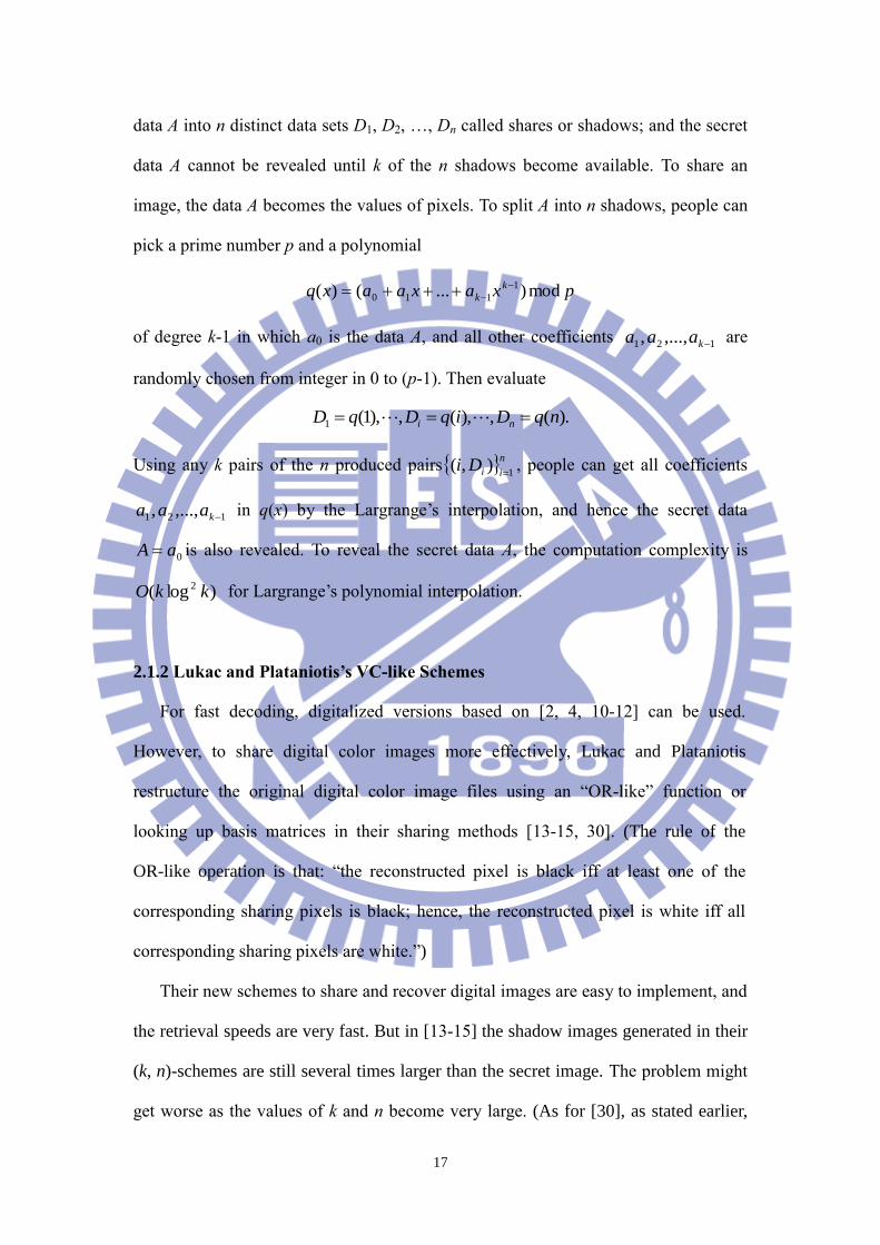
All schemes in [1, 3, 6-9] apply the polynomial interpolation to divide a secret
17
data A into n distinct data sets D1, D2, …, Dn called shares or shadows; and the secret
data A cannot be revealed until k of the n shadows become available. To share an
image, the data A becomes the values of pixels. To split A into n shadows, people can
pick a prime number p and a polynomial
pxaxaaxq k
k mod)...()( 1
110
of degree k-1 in which a0 is the data A, and all other coefficients 121 ,...,, kaaa are
randomly chosen from integer in 0 to (p-1). Then evaluate
).(,),(,),1(1 nqDiqDqD ni
Using any k pairs of the n produced pairs n
iiDi1
),(
, people can get all coefficients
121 ,...,, kaaa in q(x) by the Largrange‟s interpolation, and hence the secret data
0aA is also revealed. To reveal the secret data A, the computation complexity is
)log( 2 kkO for Largrange‟s polynomial interpolation.
2.1.2 Lukac and Plataniotis’s VC-like Schemes
For fast decoding, digitalized versions based on [2, 4, 10-12] can be used.
However, to share digital color images more effectively, Lukac and Plataniotis
restructure the original digital color image files using an “OR-like” function or
looking up basis matrices in their sharing methods [13-15, 30]. (The rule of the
OR-like operation is that: “the reconstructed pixel is black iff at least one of the
corresponding sharing pixels is black; hence, the reconstructed pixel is white iff all
corresponding sharing pixels are white.”)
Their new schemes to share and recover digital images are easy to implement, and
the retrieval speeds are very fast. But in [13-15] the shadow images generated in their
(k, n)-schemes are still several times larger than the secret image. The problem might
get worse as the values of k and n become very large. (As for [30], as stated earlier,

18
the size of each shadow images is the same as the secret image size, but [30] is for
k=n=2 only.) As a result, to store the created digital shadows often need larger storage
space in computer.
2.1.3 Wang et al.’s Fast (n, n) Scheme
Wang et al. also proposed in [17-18] some fast schemes with the intention of
small pixel expansion rate (per). Their (k, n) scheme in [17] and their first scheme (a
(2, n) scheme) in [18] are both probabilistic (and hence might be lossy in image
retrieval). Their second scheme in [18] is a deterministic (n, n) scheme for grayscale
images (extension to color images is also possible); and hence causes lossless
retrieval. Notably, in their (n, n) scheme [18], it splits a secret image A among n
shadows C1, C2, …, Cn, whose pixel expansion rate is one. After receiving all n
shadows, it uses only n-1 XOR operations to reconstruct a pixel of A. Their (n,
n)-scheme algorithm is as follows:
Coding:
Step 1. Input a secret image A.
Step 2. Generate n-1 random images B1, B2, …, Bn-1, each has size of A.
Step 3. Compute the shadows as follows:
C1=B1,
C2=B1⊕B2,
……
Cn-1=Bn-2⊕Bn-1,
Cn=Bn-1⊕A.
Step 4. Output the n shadows C1, C2, …, Cn.
Decoding:

19
Reveal A using the formula A=C1⊕C2⊕…⊕Cn.
In this chapter, in order to extend Wang et al.‟s (n, n) no-threshold scheme to (k, n)
threshold scheme; we introduce a (k, n, m) shadows-assignment matrix H, and a {B1,
B2} partition-and-recombination process. The scheme still holds the two advantages
of [18]: fast decoding speed and small pixel expansion rate. In fact, we only need
three XOR operations in average to reconstruct a pixel; and the ratio of each shadow‟s
size over the secret image‟s size is between 0 and 2, i.e. 0<per<2 (and per =2/n in the
k=n case). The statement is true in all (k, n) cases.
2.2 The Proposed Method
To generate the desired shadows, the two new techniques described in Sec. 2.2.1
and 2.2.2 will be needed in the encoding algorithm of Sec. 2.2.3. To help readers
understand the encoding, a numerical example is also given in Sec. 2.2.4.
Then, Sec. 2.2.5 introduces the decoding algorithm that retrieves the secret. For
easier understanding of the decoding algorithm; a numerical example for decoding is
also given in Sec. 2.2.6.
2.2.1 The (k, n, m) Shadows-assignment Matrix H (which has n rows and m
columns)
To design a threshold (k, n) scheme, we may first directly utilize Wang et al.‟s
non-threshold (m, m) scheme for some carefully chosen parameter
n
kCm 1 .
(The reason why m is chosen as n
kCm 1 will be explained later.) Notably, Wang et

20
al.‟s (m, m) method gives us n
kCm 1 shadows (these are not our final shadows; just
consider them as our temporary shadows). Then, we duplicate each temporary shadow
several times. Then, for the n people participating the sharing game, let each person
get one or no copy from each of the m temporary shadows. Each person can have
copies from more than one temporary shadow. However, no person can get copies
from all m shadows; otherwise, that person alone can unveil the secret.
After this distribution assignment of the copies of the m produced temporary
shadows, we wish that when any k or more people gather together in an
image-recovery meeting, the chairman of the meeting can collect all m temporary
shadows from the attendants of this meeting; and hence, can restore the secret image
according to Wang et al.‟s (m, m) image-recovery scheme. We also require that a
meeting of less than k people together is insufficient to collect all m temporary
shadows; and hence, cannot reveal the secret image. We will call the two requirements
stated above in this paragraph as the “(k, n, m) shadows-assignment requirements”.
From the idea above, we may create a matrix H of n rows and m columns. Its n
rows represent the n persons; and its m columns represent the m (distinct) temporary-
shadows produced by Wang et al.‟s deterministic (m, m) scheme. The element of H is
either 0 or 1. The ith person (row) has a copy of the jth shadow image (column) if and
only if Hij =1. In order to make the matrix meet the expected (k, n, m)
shadows-assignment requirements described above, we let each column of H have
exactly k-1 zeros and n-k+1 ones. More specifically, let H have n
kCm 1 columns, and
each column of H be a permutation of the n-dimensional basic column vector
(000…0011111…111) which has k-1 leading zeros followed by n-k+1 ones.
This obviously guarantees that: i) each temporary shadow Cj will appear at least
once when k out of the n persons attend the image-recovery meeting; ii) at least one

21
temporary shadow Cj will disappear when k-1 or fewer persons attend the recovery
meeting. The proof is as follows:
Proof: Consider the equation
T
mnmnn
m
m
T
n X
X
X
HHH
HHH
HHH
P
P
P
2
1
21
22221
11211
2
1
, (2.1)
where Pi and Hij {0, 1} (i=1, 2, …, n; j=1, 2, …, m.). In this equation, Pi
represents the attendance status of ith person (0 is absence and 1 is attendance);
and H is the created (k, n, m) shadows-assignment matrix. Therefore,
njnjjj HPHPHPX 2211 (2.2)
counts the number of times (copies) that the temporary shadow Cj appear in the
image-recovery meeting. Two observations are:
i) When k persons attend the recovery meeting, then k of the n elements in
(P1,…, Pn) are one, and the remaining n-k elements are zero. Therefore, each
Xj must be at least one, for there is exactly k-1 zeros in every column j of H.
This implies that each temporary shadow Cj will appear at least once in the
recovery meeting.
ii) When only k-1 or fewer persons attend the recovery meeting, then at most k-1
of the n elements in (P1,…, Pn) are one; or equivalently, at least n-k+1 of the n
elements in (P1,…, Pn) are zero. Let Colj = (H1j, H2j, …, Hnj) be a column of H
whose n-k+1 ones happen to appear at the positions where the vector (P1,…,
Pn) got these (at least) n-k+1 zeros. (If (P1,…, Pn) has more than n-k+1 zeros,
then just randomly choose n-k+1 positions from the zero entries of (P1,…, Pn).)
The inner product of the vector (P1,…, Pn) and this special Colj will be zero.
In other words, Xj = 0. Hence the temporary shadow Cj disappears in the

22
recovery meeting.
In the above construction of the matrix H, recall that we let all n
kCm 1
permutations of the n-dim vector (000...001111…11), which has exactly k-1 leading
zeros and n-k+1 ones, be used as the m columns; and thus obtain the expected n-by-m
matrix H. Hereinafter, the matrix H will be called the “(k, n, m) shadows-assignment
matrix”.
Below is an example showing the (k, n, m) shadows-assignment matrix H. Assume
(k, n)=(3, 4), hence 4
136 Cm . Note that each column is just a permutation of the
first column, and the first column is an n=4 dimensional vector which has exactly
k-1=3-1=2 zeros.
H =
001011
010101
100110
111000
4
3
2
1
654321
P
P
P
P
CCCCCC
. (2.3)
As a result, H has four rows (since n=4) and six columns (since 4
136 Cm ). In this
example, the person P1 owns (the copies of the) temporary shadows C4, C5, C6, the
person P2 owns temporary shadows C2, C3, C6, the person P3 owns temporary
shadows C1, C3, C5, and the person P4 owns temporary shadows C1, C2, C4. In this
shadows-assignment process, any k=3 people gather together can guarantee the
appearance of all six temporary shadows C1, C2, C3, C4, C5 and C6; but less than three
persons cannot. In other words, three or more people can recover the secret image
according to Wang et al.‟s deterministic (6, 6) scheme using these six temporary
shadows. Less than three people cannot recover because some Cj disappears.

23
2.2.2 Partition-and-recombination Process of {B1, B2}
In Sec. 2.2.1, after assigning the m temporary shadows to n people according to
the matrix H, each person gets some temporary shadows. Each person i can combine
the temporary shadows that he holds into a single shadow Di specially designed for
him. Then these n final shadows D1, D2, …, Dn owned respectively by these n persons
are the final output of a very simple (k, n)-threshold scheme.
This simplest design is easy (it only needs the idea of using the H mentioned in
Sec. 2.2.1 above, and matrix H itself is easy to construct). However, according to
Wang et al.‟s deterministic (m, m) scheme, all m temporary shadows have the same
size as that of secret image A. This often causes space-and-speed inefficiency problem.
More specifically, as n
kCm 1 becomes larger, this very simple (k, n)-threshold
scheme will have two drawbacks: (1) big-size problem for each Di of the final
shadows {D1, D2, …, Dn}; and (2) many XOR operations in decoding. In order to
avoid these two drawbacks, we do not use Wang et al.‟s output as the m temporary
shadows. Instead, we create our own m temporary shadows. This can be done by the
two-shadows partition-and-recombination preprocess proposed below.
First, create a random image B1 whose size is identical to that of the secret image
A. Then, generate another same-size image B2=B1⊕A using XOR in a bit-by-bit
manner. Notably, according to the inverse property of XOR operation, secret image A
can be recovered by the equation A=B1⊕B2. Then, create m temporary shadows C1,
C2, …, Cm by partitioning and recombining B1 and B2, as follows (see Fig. 2.1 for an
example using (k=3, n=4) ):
Step 1. Randomly generate an image B1 whose size is identical to A‟s. Then partition
B1 into n
kCm 1 non-overlapping blocks C11, C21, …, Cm1. The upper half of
each temporary shadow Ci (1≦i≦m) is the block Ci1 contained in B1.

24
Step 2. Create the security mask C*, which is also a block, by the XOR equation
C*=C11⊕C21⊕ …⊕Cm1.
Step 3. Create an image B2=B1⊕A using XOR in a bit-by-bit manner. (A, B1 and B2
have the same size.) Then partition B2 into m non-overlapping blocks C12,
C22, …, Cm2.
Step 4. For security reason, shift each Ci2 to Ci3 by the formula Ci3= Ci2⊕C*.
Step 5. After physically attaching each Ci3 to Ci1, we obtain the m temporary shadows
C1, C2, …, Cm. (Notably, the upper half of each Ci is Ci1, and the lower half of
each Ci is Ci3.)
As a remark, if B1 and B2 cannot be divided equally into m blocks of the same size,
some redundant pixels can be filled in B1 and B2. In the (k, n)=(3, 4) example, if the
size of A is 512×512, then B1 and B2 need two redundant pixels respectively, because
512×512 is not a full multiple of n
kCm 1 =6.
Fig. 2.1. A flowchart showing the process that transforms {B1, B2} to {C1, C2, …, C6}.

25
In this example, (k, n)=(3, 4); and
n
kCm 1 =6 accordingly.
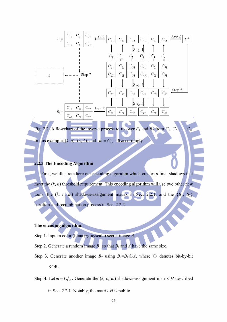
In the inverse process to obtain B1 and B2 from C1, C2, …, Cm , the algorithm is as
follows (see Fig. 2.2 where we still use (k=3, n=4) as an example):
Step 1. Extract m non-overlapping blocks C11, C21, …, Cm1 which are the upper half of
C1, C2, …, Cm , respectively.
Step 2. Recover the security mask C* by the equation C*=C11⊕C21⊕…⊕Cm1.
Step 3. Recover the random image B1 by physically attach C11, C21, …, Cm1 to each
other.
Step 4. Extract the m non-overlapping blocks C13, C23, …, Cm3 which are the lower
half of C1, C2, …, Cm , respectively.
Step 5. Recover the m blocks C12, C22, …, Cm2 using the shift-back equation Ci2= Ci3
⊕C* (where 1≦i≦m).
Step 6. Recover the image B2 by physically attaching C12, C22, …, Cm2 to each other.
Step 7. Recover the secret image A by the equation A=B1⊕B2.
26
Fig. 2.2. A flowchart of the inverse process to recover B1 and B2 from C1, C2, …, Cm.
In this example, (k, n)=(3, 4); and n
kCm 1 =6 accordingly.
2.2.3 The Encoding Algorithm
First, we illustrate here our encoding algorithm which creates n final shadows that
meet the (k, n) threshold requirement. This encoding algorithm will use two other new
tools: the (k, n, m) shadows-assignment matrix in Sec. 2.2.1, and the {B1, B2}
partition-and-recombination process in Sec. 2.2.2.
The encoding algorithm:
Step 1. Input a color (binary/grayscale) secret image A.
Step 2. Generate a random image B1 so that B1 and A have the same size.
Step 3. Generate another image B2 using B2=B1⊕A, where ⊕ denotes bit-by-bit
XOR.
Step 4. Let n
kCm 1 . Generate the (k, n, m) shadows-assignment matrix H described
in Sec. 2.2.1. Notably, the matrix H is public.

27
Step 5. Use the two images B1 and B2 to generate m temporary shadows C1, C2, …, Cm
by using the {B1, B2} partition-and-recombination process (see Sec. 2.2.2 and
Fig. 2.1).
Step 6. Assign the duplicated copies of the m temporary shadows C1, C2, …, Cm to the
n persons according to the shadows-assignment matrix H mentioned in Step 4
(see Sec. 2.2.1 for detail of the assignment). For each person i, the final
shadow Di that he has is exactly the union of those copies assigned to him.
To understand the above encoding algorithm, see the example in Sec. 2.2.4.
Remark: Each participant gets several temporary shadows which are all random
matrixes. Thus, it is better to have a discussion about how to distinguish the
temporary shadows so that the related temporary shadows inside each final shadow
can be distinguished easily later to recover the image.
Option 1. Assume that, according to the shadows-assignment matrix H, there is a
person who owns three temporary shadows {C2, C3, C6}. Let us use this person as an
example. If the size of each temporary shadow is w×h, then, before inserting the
separator, the size of this person‟s final shadow was 3w×h. (The first w rows were C2,
next w rows were C3, final w rows were C6.) Hence the number of rows of the final
shadow was three times larger than that of each temporary shadow, but the columns (h)
were the same. Now, after the first w rows, since we already finish C2, and C3 is to be
attached behind C2, we insert a separator-row of (h/2)+(h/2)=h elements, i.e.
222222222222222222222333333333333333333333, so that people can understand C2
is above this separator-row and C3 is below this separator-row. Then we store the C3
using next w rows. Then, insert another separator-row of h/2+ h/2= h elements, i.e.
3333333333333333333336666666666666666666666, before attaching C6. In

28
summary, if separators are used, the final-shadow has (3w+2) rows rather than 3w
rows, and the (3w+2) rows owned by this {C2, C3, C6} person will be
[C2] (which has w rows, each row has h pixels )
222222222222222222222333333333333333333333
[C3] (which has w rows, each row has h pixels )
3333333333333333333336666666666666666666666
[C6] (which has w rows, each row has h pixels )
Notably, in Step 4 of the encoding algorithm, we already stated that the
shadows-assignment matrix H is public, so the decoder can always read from H to
know the number of temporary shadows owned by each participant. For example, in
the H in Eq. (2.3), each participant gets 1+1+1=3 temporary shadows. Then, in Option
1, the decoder can know that the number of rows in this final shadow is 3w+(3-1)=
(3w+2). Therefore, the decoder can always figure out how many rows are in the final
shadow, and hence, know how many pixels are in each row.
Option 2 (an option using the convention of ascending-order indices.) In fact,
from the viewpoint stated in the final paragraph of Option 1 above, the separator rows
can also be omitted, as explained below. Assume each participant owns certain
shadows. Let the shadow indices be all arranged in the ascending order. For example,
if the matrix H is as shown in Eq. (2.3), then the person P1 owns (copies of the)
temporary shadows C4, C5, C6, the person P2 owns temporary shadows C2, C3, C6, the
person P3 owns C1, C3, C5, and the person P4 owns C1, C2, C4. Notice the indices are
all in ascending order (namely 4<5<6; 2<3<6; 1<3<5; 1<2<4). Therefore, even if we
do not use separators, the decoder can still read the “public” matrix H to know that

29
each participant own 3 temporary shadows; and hence, divide each person‟s final
shadow into 3 parts of equal size; and then use matrix H to identify easily which
temporary shadow is the first one-third of that person‟s final shadow, which
temporary shadow is the middle one-third, and which temporary shadow is the final
one-third.
2.2.4 Numerical Example of Encoding
In the following encoding example, we do it step by step. Without the loss of
generality, assume (k=3, n=4), so n
kCm 1 =6. Also, for easier description, we just
use gray-values rather than color-values in the example.
Step 1. Assume the given secret image is a 2×3 image
20213367
1867655A , which
has six grayscale pixel values.
Step 2. Randomly generate an image B1 whose size is identical to A‟s. For example,
randomly let
3221093
412251491B .
Step 3. Generate another image B2 by applying bit-by-bit XOR to B1 and A, i.e.
2348730
14717316212 ABB where 162=55⊕149, 173=76⊕225, etc.
Step 4. According to the skill in Sec. 2.2.1, generate a (k=3, n=4) threshold
shadows-assignment matrix
001011
010101
100110
111000
H which has n=4 rows and n
kCm 1 = 6 columns.
Note that each column is a permutation of the first column vector 0011.
Step 5. Firstly, use bit-by-bit XOR on the elements of B1 to obtain the security block
242C by the formula ]242[]32[]210[]93[]41[]225[]149[ .
Then, according to Sec. 2.2.2, generate 6 temporary shadows

30
80
1491C ,
95
2252C ,
97
413C ,
236
934C ,
165
2105C ,
24
326C where the six lower halves are the
result of transforming the six lower halves of B2, by doing bit-by-bit XOR
with 242C . For example, 80 =162⊕242, and 95 =173⊕242.
Step 6. According to the assignment matrix H, assign the copies of the m=6 temporary
shadows {C1, C2, …, C6} to the n=4 persons. Hence, our n=4 final shadows,
hold by the n=4 persons respectively, are
24165236
32210931D ,
249795
32412252D ,
1659780
210411493D ,
2369580
932251494D
where D1 and D2 both have a copy of the temporary shadow
24
326C .
2.2.5 The Decoding Algorithm
Given any k final shadows, for example the {D1, D2, …, Dk}, out of the n final
shadows produced in Step 6 of Sec.2.2.3, the secret image A can be restored as
follows:
The decoding algorithm:
Step 1. After referring to the (k, n) shadows-assignment matrix H generated in Step 4
of the encoding algorithm, we can know which temporary shadows in {C1,
C2, …, Cm} are included in each final shadow Di. Therefore, all m temporary
shadows C1, C2, …, Cm can be extracted from these k final shadows. (For the
reason, reader can see the (k, n, m) shadows-assignment requirements in Sec.
2.2.1, and the proof near Eq. (2.2).
Step 2. Use all m temporary shadows C1, C2, …, Cm to generate B1 and B2 by

31
implementing the inverse process of the {B1, B2}-partition-and-recombination
process (see Sec. 2.2.2 and Fig. 2.2).
Step 3. Reveal the secret image A using A=B1⊕B2.
Remark: Step 1 above stated that we can know which temporary shadows in {C1,
C2, …, Cm} are included in each final shadow Di. As for how to distinguish the
temporary shadows in each final shadow Di (so that the related temporary shadows
inside each final shadow Di can be distinguished easily to recover the image), see the
Remark at the end of Sec. 2.2.3.
2.2.6 Numerical Example for Decoding
In the following decoding example, still assume (k=3, n=4). As a result, decoding
needs any 3 of the 4 final shadows. Without the loss of generality, assume D1, D2, D3
are the three available shadows.
Step 1. With the help of the matrix H in Step 4 of encoding process, we extract
all n
kCm 1 = 6 temporary shadows C1, C2, …, C6, which are the same as those
created in Step 5 of encoding process of Sec. 2.2.4.
Step 2. Recover B1 and B2, which are the same as those in Steps 2 and 3 of the
encoding process, by implementing the inverse process of the {B1, B2}
partition-and-recombination process to all six temporary shadows C1, C2, …,
C6 (see Fig. 2.2).
Step 3. Reveal the secret image A by
20213367
186765521 BBA .

32
2.3 Experimental Results
In our experiment, the input color image A is the popular test-image shown in Fig.
2.3(a). For (k, n)=(2, 4) case, the n=4 final shadows D1, D2, D3, D4 generated in Sec.
2.2.3 are shown in Fig. 2.3(b-e), and each has size 2×(n-k+1)/n=2×(4-2+1)/4=3/2
times larger than size of A. Fig. 2.3(f) shows the error-freely recovered A using any
k=2 of the four final shadows.
Other experiments dealing with (k, n)=(3, 4) and (k, n)=(4, 4) cases are shown in
Fig. 2.4 and 2.5 respectively. And their pixel expansion rates are 2×(n-k+1)/n=2×
(4-3+1)/4=1 and 2×(n-k+1)/n=2×(4-4+1)/4=1/2, respectively.
To show our constant decoding-time property, we also record in Figures 2.6 and
2.7 the actual CPU time taken in decoding. The computer used is an IBM laptop with
an Intel Pentium 1.70GHz CPU, and the operating system is Microsoft Window XP
SP2. From Fig. 2.6, which deals with (n, n) system, it can be seen that our decoding
time really does not vary as the value of n varies, but this is not the case for Wang et
al‟s scheme [18]. Notably, for all (k, n) systems, our decoding time still remain
constant as n increases its value. An example showing this is given in Fig. 2.7 in
which k=n/2. Note that Wang et al‟s [18] does not have (k, n) systems unless k is n or
2.
(a)

33
(b) (c)
(d) (e)
(f)
Fig. 2.3. An example of (k=2, n=4). Here, (a) is the given 24-bit-per-pixel color image
A; (b-e) are our final shadows D1, D2, D3, D4; (f) is the recovered error-free A using
any two of the four final shadows.

34
(a) (b)
(c) (d)
(e)
Fig. 2.4. An example of (k=3, n=4). Here, (a-d) are our final shadows D1, D2, D3, D4 ;
(e) is the recovered error-free A using any three of the four final shadows.
(a) (b)

35
(c) (d)
(e)
Fig. 2.5. An example of (k=4, n=4). Here, (a-d) are our final shadows D1, D2, D3, D4 ;
(e) is the recovered error-free A using all four final shadows.
0
20
40
60
80
100
120
140
160
180
200
10 20 30 40 50 60 70 80 90 100
n
millisecond Proposed Scheme
Wang's Scheme [18]
Fig. 2.6. The CPU time (milliseconds) for decoding (n, n) systems.

36
0
20
40
60
80
100
120
140
160
180
200
10 20 30 40 50 60 70 80 90 100
n
millisecond Proposed Scheme
Fig. 2.7. The CPU time (milliseconds) for decoding each (n/2, n) systems by our
scheme. There is no curve for Wang et al‟s scheme [18], for their scheme has no (n/2,
n) system or other (k, n) systems when 2≦k<n.
2.4 Discussions
2.4.1 Recoverability and Security
In general, each (k, n) threshold secret sharing scheme must satisfy both
requirements: the recoverability (any k or more shadows can reveal all information of
A) and the security (any k-1 or fewer shadows cannot reveal the secret image A).
In our scheme, when any k out of the n final shadows are gathered (for example,
D1, D2, …, Dk), the secret image A is revealed by Steps 1-3 of the decoding algorithm.
These steps also explain why our scheme satisfies the recoverability requirement.
Firstly, if k or more final shadows are gathered, then we can extract all m temporary
shadows C1, C2, …, Cm from the k available final shadows according to the (k, n, m)
shadows-assignment requirements of the matrix H. Secondly, after physically dividing
each Ci into upper half Ci1 and lower half Ci3, we can get C* which is defined by

37
C*=C11⊕C21⊕ …⊕Cm1. Then, we can restore C12, C22, …, Cm2 using Ci2= Ci3⊕C*
for each i=1,…,m. Then recover B1={C11, C21, …, Cm1} and B2={C12, C22, …, Cm2}.
Therefore, the secret image A can be revealed using A=B1⊕B2.
Our scheme also satisfies the security requirement. Assume that only k-1 or fewer
final shadows are available. Then, according to the (k, n, m) shadows-assignment
requirements of the matrix H, people cannot obtain all m temporary shadows C1,
C2, …, Cm from these final shadows (see the proof (ii) below Equation (2.2) of Sec.
2.2.1). Assume Cq is missing. As a result, people cannot obtain C* defined by C*=C11
⊕C21⊕ …⊕Cm1 , due to the lack of the Cq1 which is the upper half of Cq. Then,
without C*, people cannot restore C12, C22, …, Cm2 defined by Ci2= Ci3⊕C* (1≦i≦
m). Therefore, people cannot generate B2. As a result, the secret image A=B1⊕B2
cannot be revealed due to absence of B2.
Below we discuss the probability of obtaining the right secret image A through
guessing. Without the loss of generality, assume that a betrayal party of k-1 persons
already gathers m-1 temporary shadows C1, C2, …, Cm-1 without Cm. Notably, A={Ai |
1≦i≦m}, i.e. image A can be divided to m blocks, and the recovery of A can be done
block by block; in other words, since A=B1⊕B2 , we have
Ai= Ci1⊕Ci2= Ci1⊕(Ci3⊕C* )= Ci1⊕Ci3⊕(C11⊕C21⊕…⊕Cm1), 1≦i≦m.
Because of the lack of Cm = [Cm1 | Cm3]T, the betrayal party will have to guess a value
for a pixel in Cm1, then they use this guessing value to get a set of m-1 pixels‟ values
(one value per block in A1, A2, …, Am-1). Then they need to guess the value of a pixel
at the corresponding position of Cm3 (or Am) so that the pixel value at that position of
Am can also be shown. The above is just to recover a pixel (for example, the
top-leftmost pixel) of each block Ai ,1≦i≦m. This value-guessing of two pixels will
repeat bksize times. Here, bksize is the size of each block Ai (1≦i≦m); hence bksize
is m times smaller than image size of A.

38
From the description above, we can evaluate the probability of obtaining the right
color image A with size w×h as follows. (For illustration, still assume (k, n)=(3, 4);
hence n
kCm 1 =6 accordingly.)
2
24
31 )2
1()
pixelscale
1()
pixelscale
1(yProbabilit
m
hw
m
hw
m
hw
bksizebksize ss which is
631304
24241087381)
2
1(3/512512)
2
1(
if the image size is w×h = 512512 . Here,
s=1/224
is the probability to guess successfully a pixel‟s value; bksize1 is the number
of pixels in Cm1; and bksize3 is the number of pixels in Cm3. To improve the security
further, people can use a prime number as a key (a seed) of a random number
generator to rearrange the pixel positions in the secret image A (as Thien and Lin did
in [6]) before encoding.
2.4.2 Time Complexity and Storage Space Needed
In terms of computation complexity, Thien and Lin‟s polynomial sharing scheme
[6] needs O(log2k) mathematical operations to reveal a pixel. Although Wang and Su
[3] reduced 40% in size of Thien and Lin‟s shadow images, their scheme still need
O(log2k) mathematical operations to reveal a pixel. As for the digitalized versions
derived from [4, 10-12], they need O(k×per) OR operations to reveal a pixel. Here, the
value k means the secret-recovery requires k gathered shadows, and the value per
represents pixel expansion rate (per≧2 in [4, 10-12]). Lukac and Plataniotis‟s
methods [13-15] also need O(k×per) “OR-like” operations to restore an original input
pixel in (k, n)-threshold schemes. Lukac and Plataniotis‟s special method [30] needs
only 1 B-bit “OR-like” operation to restore a pixel of B-bit color secret image, but [30]
only deals with the k =2=n scheme. Fang and Lin [50] proposed two other SS (sharing
schemes), i.e. an (n, n) XOR-SS and a (k, n) OR-SS, to reduce the size of shadows in
Lukac and Plataniotis‟s [15]. But the (k, n) OR-SS scheme in [50] still needs many

39
OR operations in decoding, and the complexity is similar to that of Wang et al.‟s (k, n)
colored probabilistic scheme [17]. In Wang et al.‟s (n, n) scheme [18], it only needs
n-1 XOR operations to reconstruct each pixel, which is the same as Fang and Lin‟s (n,
n) XOR-SS scheme [50]. Obviously, the decoding time of most inventions above
increases as the value of k or n increases.
For this concern, our new scheme tries to make the speed of Wang et al.‟s [18]
more stable for any n. In any (k, n) threshold cases, no matter how large the value of n
is, we only needs at most three bit-by-bit XOR operations to restore a pixel. Notably,
each XOR is between a pair of 24-bit values if the image is color.
To see this, assume that the size of secret image A is w×h, then the number of
XOR operations needed to evaluate C*=C11⊕C21⊕ …⊕Cm1 is (m-1)×[(w×h)/m]<w
×h because each Ci1 has size [(w×h)/m]. Then, to get C12, C22, …, Cm2, it needs m×[(w
×h)/m]= w×h XOR operations to evaluate Ci2= Ci3⊕C*, here 1≦i≦m. Finally, to
reveal A, it needs w×h XOR operations to evaluate A=B1⊕B2. Together, it needs [(3×
m-1)/m]×(w×h)<3×(w×h) XOR operations to reveal A from any k final shadows. In
average, since image A has w×h pixels, it needs at most three XOR operations to
restore each pixel. Table 2.1 below shows a comparison with reported schemes.
Obviously, the proposed scheme has the smallest decryption load in average. Notably,
the proposed scheme also needs at most three XOR operations in encoding process to
share each pixel of secret image into the n final shadows D1, D2, …, Dn, because the
decoding process is exactly an inversion of encoding one. Besides Table 2.1, the
readers can also read Figures 2.6 and 2.7 to see that our decoding time does not
increase as n increases its value. Since, besides our method, Wang‟s [18] is one of the
fastest schemes in Table 2.1, we only compare our CPU time with [18] in Fig. 2.6. As
for Fig. 2.7, because [18] has no (k, n) design if 2<k<n, no curve for [18] is drawn
there. (We only use this figure to show that our CPU time is really a constant.)

40
Table 2.1. Time complexity for decoding. (The time to reconstruct a pixel of image
A.)
Schemes (k, n) threshold (n, n) threshold
Thien and Lin‟s
polynomial scheme
[6]
O(log2k) (Math operations
(1)) O(log
2n) (Math operations)
Wang and Sue‟s
polynomial scheme
[3]
O(log2k) (Math operations) O(log
2n) (Math operations)
Digitalized version of
[4, 10-12]
O(k×per (2)) (OR operations) O(n×per) (OR operations)
Lukac and
Plataniotis‟s schemes
([13-15, 30])
O(k×per) (OR-like
operations) for [13-15].
([30] is for (2, 2) case only;
there is no (k, n) case in
[30].)
O(n×per) (OR-like
operations) for [13-15].
([30] is for (2, 2) case only,
and it needs only 2-1=1
OR-like operation.)
Fang & Lin‟s scheme
[50]
O(k×per) (OR operations) n-1 (XOR operations)
Wang et al.‟s scheme
[17-18]
O(k×per) (OR operations) in
Ref. [17].
[18] gave no (k, n) scheme(3)
unless k=2; and its (2, n)
scheme uses only 2-1=1
O(n×per) (OR operations) in
Ref. [17].
n-1 (XOR operations) in Ref.
[18].

41
XOR operation to
reconstruct a pixel of A.
Our scheme 3 (XOR operations) 3 (XOR operations)
(1) Math operations: +, -, ×, ÷.
(2) Note that per means “Pixel expansion rate”. Usually, per is a positive integer at
least two in [4, 10-15, 17, 50].
(3) When k=2, the (2, n) scheme in [18] is a very fast one, for only one XOR operation
is needed. But their decoding is not lossless.
As for the space complexity, Thien and Lin‟s scheme [6] has a pixel expansion
rate per=1/k for the (k, n) threshold cases. Wang and Su proposed the scheme [3] to
reduce 40% of Thien and Lin‟s shadow images size. On the other hand, as the value of
n increases, the per is very large for digital versions of schemes [4, 10-12]. Although
the probabilistic scheme [16] has per=1, the reconstructed secret image is not
error-free. The per in Lukac and Plataniotis‟s schemes [13-15] are at least two. Lukac
and Plataniotis‟s special method [30] has no pixel expansion problem (per=1), but it is
only for (2, 2) scheme. Although Fang and Lin‟s (n, n) and (k, n) schemes [50] have
shadows of size smaller than Lukac and Plataniotis‟s [15], their (k, n) scheme still has
a per larger than one. The per in Wang et al.‟s colored probabilistic (k, n) scheme [17]
is still not less than one (per≧1). As for Wang et al.‟s deterministic (n, n) scheme [18],
the per is one; but [18] does not have (k, n) schemes unless k=2.
In the proposed scheme, our per is between 0 and 2; moreover, close to 0 is
possible. To see this, let the size of secret image A is w×h. Since the size of every
temporary shadow Ci (1≦i≦m) is 2×(w×h)/m, the size of every final shadow Di (1≦i
≦n) is

42
nknhw
CChwCmhw n
k
n
k
n
k
/
//
)1)((2
])(2[])(2[ 1
11
1
1
.
Here, we have used the fact that each final shadow Di contains 1
1
n
kC temporary
shadows. Now, after dividing the above by the size of A, we get our pixel expansion
rate, i.e.
per = 2×(n-k+1)/n < 2, true for any (k, n). (2.4)
Therefore, each final shadow will be at most two times larger than the secret image A.
When n is very large and k is two, the rate converges to its upper bound 2. On the
other hand,
per < 1 if k > 1+n/2. (2.5)
In the special case when k=n, our per is 2/n, and hence,
per= 2/n 0 if k=n∞. (2.6)
Therefore, each shadow will be very small when k=n. (See Fig. 2.5 for example in
which per= 2/n=2/4=0.5 because n was only 4. If we had used a very large n, then the
per would have been much smaller.)
In summary, the proposed scheme does not have a serious pixel expansion
problem or huge storage-space demanding for shadows (see Table 2.2).
Table 2.2. Comparison of the pixel expansion rate (per) when shadows are created.
Schemes (k, n) threshold (n, n) threshold
Thien and Lin‟s
polynomial scheme
([6])
1/k 1/n
Wang and Sue‟s
polynomial scheme
([3])
(1/k)×60% (1/n)×60%

43
Digital versions of [4,
10-12]
per is at least 2. per is at least 2
Lukac and Plataniotis‟s
schemes [13-15, 30]
per is at least 2.
(per =1 in [30], but [30] is
for (2, 2) case only.)
per is at least 2.
(per =1 in [30], but [30] is
for (2, 2) case only.)
Fang & Lin‟s scheme
[50]
m×n/(n+1)
for some integer m≧2.
n/(n+1)
Wang et al.‟s scheme
[17-18]
per≧1 in Ref. [17].
(Ref. [18] gave no (k, n)
scheme unless k=2; and per
= 1 in its (2, n) scheme.)
per≧1 in Ref. [17].
(per =1 in (n, n) scheme Ref.
[18].)
Our scheme 0<per =2×(n-k+1)/n<2 0<per =2/n≦1
2.4.3 Lossless Reconstruction and Core Works in Implementation
Table 2.3 provides the information about lossless reconstruction. Most of
schemes mentioned here are lossless in recovery, including our scheme. Exceptions
are the digitalized versions of [4, 12, 17], and the (2, n) scheme of [18] when 2<n.
Table 2.3. Comparison of the perfect reconstruction ability.
Schemes (k, n) and (n, n)
Thien and Lin‟s
polynomial scheme ([6])
Lossless recovery
Wang and Sue‟s
polynomial scheme ([3])
Lossless recovery
Digitalized versions of [10, 11] are lossless, but [4, 12] are lossy.

44
[4, 10-12]
Lukac and Plataniotis‟s
schemes [13-15, 30]
Lossless recovery
Fang & Lin‟s [50] Lossless recovery
Wang et al.‟s scheme
[17-18]
Recovery might be lossy in [17] if per is close to 1.
The (2, n) scheme of [18] is lossy. ([18] gives no (k, n)
scheme unless k=2.) The (n, n) scheme of [18] is
lossless.
Our scheme Lossless recovery
Finally, Table 2.4 gives the information about the kinds of work to implement
each scheme. In summary, [3, 6-9] evaluated polynomials and the remaining schemes
used OR-like operations, or XOR operations, or Look-Up-Tables.
Table 2.4. The main work being used in coding/decoding for each scheme.
Schemes Encoding Decoding
Thien and Lin‟s
polynomial scheme
([6])
Evaluate a polynomial Use Largrange‟s
interpolation.
Wang and Sue‟s
polynomial scheme
([3])
Evaluate a polynomial Use Largrange‟s
interpolation.
Digitalized versions of
[4, 10-12]
Either look up the basis
matrices or use OR
operations.
Either look up the basis
matrices or use OR
operations.

45
Lukac and
Plataniotis‟s schemes
[13-15, 30]
Either look up the basis
matrices or use OR-like
operations.
Either look up the basis
matrices or use OR-like
operations.
Fang & Lin‟s scheme
[50]
Either look up the basis
matrices or use OR-like
operations.
Use XOR operations.
Wang et al.‟s scheme
[17-18]
[17] either looks up the
basis matrices or uses OR
operations.
[18] uses {AND, XOR}
operations in the first
scheme; uses XOR
operations in the second
scheme.
[17] either looks up the basis
matrices or uses OR
operations.
[18] uses XOR operations
in both first and second
schemes.
Our scheme Use XOR operations. Use XOR operations.
2.5 Summary
In polynomial-based sharing approach, the shadow size is never a problem, but the
decoding speed is very slow due to the polynomial-interpolation evaluation. To the
contrary, storage space for shadows is large for almost all fast methods (the pixel
expansion rate per is usually at least 2 for (k, n)-threshold schemes, and per=1 is
limited to lossy schemes or some (n, n) non-threshold schemes.) In this chapter, we
have designed successfully a scheme so that: 1) the generated shadows are with
reasonable size. The per is between 0 and 2; and close to 0 when k is large and close
to n [see Eq. (2.4-2.6)] (our per=2/n in all (n, n) schemes); 2) the scheme only needs

46
three 24-bit XOR operations per pixel to get a recovery of the given color image; and
3) unlike some probabilistic approaches, our recovered images are lossless; 4) our
scheme is missing-allowable because it is a (k, n)-threshold scheme which requires
only k out of the n shadows appear in the recovery meeting.
We have implemented the cases with (k, n) being, respectively, (2, 2), (2, 3), (3, 3),
(2, 4), (3, 4), (4, 4), etc. The results are satisfactory in terms of the above advantages.
Notably, the method also works for binary or grayscale image because the method is
based on bit-by-bit operation. In fact, the given secret image A can be B-bit per pixel
for any positive integer B (for example, use B=1 for binary image, B=7 or 8 for
grayscale image, B=15 for 5-5-5 pseudo-color image, B=24 for 8-8-8 color image).
47
Chapter 3
Single Image Sharing with User-friendly Shadows
and Progressive Decoding
In this chapter, we propose a novel sharing method with n user-friendly shadows
and progressive decoding based on modulus operations. First, a fundamental (n, n)
sharing version based on modulus operations is introduced. This simple version is
neither user-friendly, nor progressive. Then, the fundamental version is extended to an
intermediate version with user-friendly shadows by using a smaller value m in the
modulus operations, although the intermediate version is still non-progressive. Finally,
the final version is proposed by extending the intermediate (user-friendly) version
further to the one with both progressive decoding and user-friendly features.
The remaining portion of this chapter is organized as follows. Section 3.1 briefly
describes Fang‟s user-friendly progressive sharing method [19]. Section 3.2 presents
the proposed method. Experimental results and some comparisons are shown in
Section 3.3. Finally, the summary is in Section 3.4.
3.1 A Simple Review of Fang‟s Method [19]
This section reviews roughly Fang‟s progressive and user-friendly method [19].
His method is for binary (black or white) images; therefore, bit-plane by bit-plane
processing is required when input image is grayscale or color. His sharing and
recovering algorithms are as follows:

48
Sharing phase: (see Fig. 3.1 for the sharing phase of Fang‟s method [19]):
Step 1. According to the two leftmost columns of Table 3.1, expand every pixel of the
black-or-white input image O to a 2×2 block in the corresponding position of
the expanded image O'. Notably, if the input pixel is black, then all pixels of
the corresponding 2×2 block are black. Conversely, if the input pixel is white,
then the corresponding 2×2 block contains two white and two black pixels (in
this case, the corresponding 2×2 block is randomly selected from the six
possibilities listed in lower part of column O' in Table 3.1).
Step 2. For each 2×2 block of the expanded image O', by checking the pixel value at
the corresponding position of a given stego-image T, Fang randomly picked up
one of the corresponding patterns listed in the rightmost column of Table 3.1
to create the 2×2 sharing block at the corresponding position of first shadow S1.
Similar argument created each of the remaining n-1 shadows.
Fig. 3.1. The sharing phase of Fang‟s method [19].

49
Table 3.1 Fang‟s selection of sharing patterns in [19]. (See Fig. 3.1 to understand O,
O' and T)
Secret pixel
O(x, y)
Expanded
secret O'
Cover pixel
T(x, y)
Possible choices for the related
2-by-2 block of a share Si (1in)
B(1)
(B,B,B,B)
B
(B,B,W,W),(B,W,B,W), (B,W,W,B),
(W,B,B,W), (W,B,W,B), (W,W,B,B)
W
(W,W,W,W),(B,W,W,W),(W,B,W,W),
(W,W,B,W), (W,W,W,B)
W (B,B,W,W) (2)
B (B,B,W,W)
W (W,W,W,W), (B,W,W,W), (W,B,W,W)
(B,W,B,W) B (B,W,B,W)
W (W,W,W,W), (B,W,W,W), (W,W,B,W)
(B,W,W,B) B (B,W,W,B)
W (W,W,W,W), (B,W,W,W), (W,W,W,B)
(W,B,B,W) B (W,B,B,W)
W (W,W,W,W), (W,B,W,W), (W,W,B,W)
(W,B,W,B) B (W,B,W,B)
W (W,W,W,W), (W,B,W,W), (W,W,W,B)
(W,W,B,B) B (W,W,B,B)
W (W,W,W,W), (W,W,B,W), (W,W,W,B)
(1) „B‟ represents black pixel; „W‟ represents white pixel.
(2) Each 2×2 block in the expanded image O' (or in each shadow Si) is represented as
(left-up pixel, right-up pixel, left-bottom pixel, right-bottom pixel).

50
Recovering phase: (see Fig. 3.2 for Fang‟s experimental result)
Assume that k shadows are collected. Then, each pixel j of the black-or-white image
is reconstructed using the k sharing pixels at the same position j of the k shadows. The
reconstruction rule is an OR-like operation: “the reconstructed pixel is black iff at
least one of the k sharing pixels is black.” (Hence, the reconstructed pixel is white iff
all k sharing pixels are white.)
Fig. 3.2. Experimental result of the recovering phase in Fang‟s method: (a) one of the
six (n=6) user-friendly shadows; (b-f) the reconstructed results using 2-6 shadows,
respectively.
Fang‟s method has two disadvantages: i) The size of each shadow Si is four times
larger than the input image O because the sharing patterns in Step 2 of sharing phase
are 2×2 blocks (see the fourth column of Table 3.1); ii) The image quality (such as
PSNR) of shadows is not easy to control. We will improve them in this chapter.
51
3.2 The Proposed Method
This section presents our user-friendly progressive sharing method based on
modulus operations. The method generates n user-friendly shadows whose image
quality (such as PSNR) is lower than the input image‟s quality; and later, the input
image can be reconstructed with progressively-improved image quality after gathering
k (2kn) shadows. The description of the method is divided into three subsections.
First, a fundamental (n, n) sharing version based on modulus operations is introduced
in Sec. 3.2.1. This simple version is neither user-friendly, nor progressive. Then, the
fundamental version is extended in Sec. 3.2.2 to an intermediate version with
user-friendly shadows, although the intermediate version is still non-progressive.
Finally, Sec. 3.2.3 presents the final version by extending the intermediate
(user-friendly) version further to the one with both progressive decoding and
user-friendly features. A comparison between our progressive and user-friendly
method (Sec. 3.2.3) and Fang‟s (Sec. 3.1) is in Sec. 3.2.4. A stego version of our
method is in Sec 3.2.5.
3.2.1 An (n, n) Fundamental Sharing Version Based on Modulus Operations
This sub-section illustrates a fundamental (n, n) sharing version for grayscale
images based on modulus operations. This version splits a grayscale image A among
n extremely noise-like shadows B1, B2, …, Bn whose sizes are all the same as A. The n
noise-like shadows together can reconstruct each pixel of A by using one modulus
operation and n-1 addition. (In this dissertation, “+” and “Mod” denote addition
and modulus operations, respectively.) The sharing and recovering phases of the
fundamental version are listed below.

52
Sharing phase:
Step 1. Input a grayscale secret image A.
Step 2. Generate n-1 random images B1, B2, …, Bn-1 as shadows. Each is as large as
A.
Step 3. Create the nth
shadow Bn by
Bn = {A+(256-[(B1+B2+…+Bn-1)Mod 256])}Mod 256. (3.1)
Step 4. Output the n noise-like (non-friendly) shadows B1, B2, …, Bn.
Recovering phase:
Retrieve A using the formula
A=(B1+B2+…+Bn)Mod 256. (3.2)
Notably, both “+” and “Mod” are pixel-by-pixel operations. This sharing scheme
also can work for binary or color images by using 2(=21) and 16777216(=2
24),
respectively, to replace the constant 256 in the two formulas above. An experimental
result using the grayscale image Lena as image A is shown in Fig. 3.3, with (n, n)=(4,
4).

53
(a)
(b) (c) (d) (e)
(f)
Fig. 3.3. An example of the (n, n) fundamental sharing version introduced in Sec 3.2.1.
Here, (n, n)=(4, 4); (a) is the given grayscale image Lena A; (b-e) are the four
generated “non-friendly” shadows B1, B2, B3, B4; (f) is the recovered error-free Lena
using formula A=(B1+B2+B3+B4)Mod 256.
3.2.2 A User-friendly but Non-progressive (n, n) Version
This sub-section describes how to extend the (n, n) fundamental version in Sec.
3.2.1 to an intermediate version whose n shadows are all user-friendly, i.e. look like
visual-quality-reduced versions of the natural image, so that the management of the n
shadows is easier. What we do is to use a smaller value m to replace the value 256 in
the modulus operations in Sec. 3.2.1. Notably, the version in Sec 3.2.2 here is still

54
non-progressive.
Sharing phase:
Step 1. Input an integer parameter m (2m256) and an 8-bit grayscale image A.
Generate a smaller-range image
A' = (A)Mod m (3.3)
whose size is identical to A, but with pixel value less than m (rather than 256).
Step 2. Generate n-1 “random” images 121 ,,, nBBB whose sizes are all as large as
A; but each pixel is a random value chosen from {0, 1, 2, …, (m-1)}. Then
create
nB = {A'+(m-[( 1B+ 2B+…+ 1nB )Mod m])}Mod m (3.4)
which implies that ( 1B+ 2B+…+ nB )Mod m = A'.
Step 3. Output the n user-friendly shadows {B1, …, Bn} defined by
Bi = (A-A')+iB for i=1,…,n. (3.5)
Recovering phase:
Retrieve A by
A=[Bi-(Bi)Mod m]+[(B1+B2+…+Bn)Mod m]. (3.6)
In Eq. (3.6), it does not matter which one of B1, B2, …, Bn is used as Bi; the result
is the same. Also, if m=256 is used in Eq. (3.3)-(3.6), then this intermediate version is
identical to the (n, n) sharing one in Sec. 3.2.1.
3.2.3 The User-friendly and Progressive Version
The intermediate version (Sec. 3.2.2) is still non-progressive, although

55
user-friendly. Sec. 3.2.3 extends the intermediate version so that progressiveness is
also equipped with. The algorithm is presented here step by step. Because the version
is an extension of Sec. 3.2.2, the modulus-base notation m (2m256) is still used
here in Sec. 3.2.3. The new version can generate n friendly shadows and reconstruct
the input image in a progressive manner, i.e. the reconstructed quality improves as the
number of gathered shadows increases.
Sharing phase:
Step 1. Input an integer parameter m (2m256) and an 8-bit grayscale secret image A
(A can also be one of the three 8-bit color-components of a 24-bit color
image).
Step 2. By a pixel-by-pixel manner, generate a smaller-range image
A' = (A)Mod m (3.7)
whose size is identical to A, but pixel value is at most m-1, rather than 255.
Step 3. Generate n-1 random images R1, R2, …, Rn-1. (Each image Ri is as large as A,
and each pixel of Ri is 8-bit.)
Step 4. Create n images nBBB ,,, 21 in a pixel-by-pixel manner:
If A'=0 then 1B= 0; else 1B= (R1)Mod )1( A . Anyway, define 1A=A'- 1B .
If 1A=0 then 2B =0; else 2B =(R2)Mod )1( 1 A . Anyway, define 2A = 1A- 2B .
...
If 2
nA =0 then 1
nB =0; else 1
nB =(Rn-1)Mod )1( 2
nA . Anyway, define
1nA = 2
nA - 1
nB . Finally, let nB = 1
nA .
Step 5. Output n final shadows B1, B2, …, Bn defined by
Bi = (A-A')+ iB for i=1,…,n. (3.8)
(In Step 4 of the sharing phase above, “ 1B =(R1)Mod )1( A ” means that

56
“ 1B (t)=(R1(t))Mod )1( tA ” at pixel t. Then, after creating 1B (t), we create 1A (t)
by the formula 1A (t)=A'(t)- 1B (t). The explanation for the remaining operations
in Step 4 is likewise.) Notably, as t changes, for random effect, we randomly
switch the order of assigning these computed values to { )(,),(),( 21 tBtBtB n }.
For example, when t=0, assign the computed values to )(,),(),( 21 tBtBtB n as
above, respectively; then, when t=1, assign the computed values to
),(,),(),( 11 tBtBtB nn
respectively; then, when t=2, …. Here, we may use a
random number generator to create the permutation order for this.
Recovering phase:
After gathering any k (2kn) shadows
Bi(1), Bi(2), …, Bi(k) (1i(j)n for 1jk),
which are subset of the n shadows {B1, B2, …, Bn}, retrieve A using the formula
A~
= [Bi(j)-(Bi(j))Mod m]+[(Bi(1)+Bi(2)+…+Bi(k))Mod m]. (3.9)
Here, Bi(j) can be any one of Bi(1), Bi(2), …, Bi(k).
Lemma 1. In Eq. (3.9), anyone in Bi(1), Bi(2), …, Bi(k) can be used as Bi(j) .
Proof. Eq. (3.8) implies
Bi- iB = A-A' for all i=1,…,n, (3.10)
hence we have (Bi(j)- )( jiB )Mod m = (A-A')Mod m for all 1i(j)n for 1jk. However,
(A-A')Mod m=0 because A' =(A)Mod m by Eq. (3.7). Therefore, (Bi(j)- )( jiB )Mod m=0. So
(Bi(j))Mod m = ( )( jiB )Mod m = )( jiB (3.11)
where the last identity is due to the fact that )( jiB <(A'+1) by Step 4 above, and the
range of A' is {0, …, m-1} by Eq. (3.7). We may thus say that

57
Bi(j)-(Bi(j))Mod m = Bi(j)- )( jiB = A-A' (Here, 1i(j)n for 1jk). (3.12)
-END of Proof-
Lemma 2. In Step 4 of the sharing phase above,
A' = 1B+ 2B+…+1nB +
nB . (3.13)
Proof. Because 1A= A'- 1B , we have A' = 1B+ 1A .
Because 2A = 1A- 2B , we have A' = 1B+ 1A= 1B+ 2B+ 2A .
Because 3A = 2A- 3B , we have A' = 1B+ 2B+ 3B+ 3A .
…
Because 1nA =
2nA -
1nB , we have A' = 1B+ 2B+…+
1nB +
1nA .
Finally, because nB = 1nA , we have A' = 1B+ 2B+…+
1nB + nB .
-END of Proof-
Lemma 3. When all n shadows are received, i.e. when k=n, then A can be recovered
losslessly by Eq. (3.9). In other words,
A = [Bi-(Bi)Mod m]+[(B1+B2+…+Bn)Mod m]. (3.14)
(Again, it does not matter which one of {B1, B2, …, Bn } is used as the Bi.)
Proof. Below we show why the recovery image A~
becomes the original image A
when k=n. Since k=n, Equations (3.9), (3.12), and (3.13) imply
A~
= [Bi(j)-(Bi(j))Mod m]+[(Bi(1)+Bi(2)+…+Bi(n))Mod m]
= [Bi-(Bi)Mod m]+[(B1+B2+…+Bn)Mod m]
= [A-A']+[(B1)Mod m+(B2)Mod m+…+(Bn)Mod m]Mod m
= [A-A']+[ 1B+ 2B+…+ nB ]Mod m
= [A-A']+[A']
= A -END of Proof-

58
Step 4 above implies each pixel of nBBB ,,, 21 is non-negative because each
pixel is created by a modulus function. Moreover, in Step 4 above, the pixel values of
A' is distributed randomly among 1B , 2B , …,nB ; and Eq. (3.13) reads
1B+ 2B+…+1nB +
nB = A'
in which all pixel values are non-negative; hence, to estimate the image quality
(PSNR) of shadows B1, B2, …, Bn, we may start from the rough estimation
n
ABi
. (3.15)
Now, the root-mean-square error (RMSE) for each iB (1in), as compared with the
input image A, is defined as
tCount
tBtA
BRMSEtall
i
i
2
. (3.16)
Here, A(t) is a pixel value in A, and tBi is in iB . By Eq. (3.8), iBRMSE is
evaluated as
tCount
tBtAtAtAtall
i 2
, which can be reduced as
tCount
n
ntA
tall
2
)1(
by Eq. (3.15). Because n
n )1( is a given
constant due to the known value of n, the above rough estimation of iBRMSE can
be re-written as
n
n
tCount
tAtall )1(
2
. Although the actual value of
tCount
tAtall
2
depends on the histogram of the image A', we may roughly estimate
tCount
tAtall
2
as
73.1/)1()1/()(
1
0
2
mmdtt
m
(3.17)

59
which is the probabilistic average value considering the fact that
)1(,,1,0 mtA . Therefore, we have
n
nmBRMSE i
73.1
)1()1(. (3.18)
Then, we can get the rough estimation
2
2
102
2
10
73.1
)1()1(
255log10
255log10
n
nmBRMSEBPSNR
i
i . (3.19)
Some experimental results of iBPSNR are shown in Table 3.2, which uses five
nature images in Fig. 3.3(a) and Fig. 3.4. From this table, we can see that the
experimental value of PSNR is close to the estimation given by Eq. (3.19).
In our experiments, for the same value k, all reconstructed images have similar
PSNR values. For example, in each of the three experimental results of Fig. 3.5, 3.6
and 3.7, the four images respectively reconstructed by shadows {B1, B2, B3} (or by
{B1, B2, B4} , or by {B1, B3, B4}, or by {B2, B3, B4}) all have very similar PSNR
values. Likewise, the six images reconstructed by any two shadows of {B1, B2, B3, B4}
also have similar PSNR values. In recovering phase, when more shadows are
gathered (k becomes larger), then the reconstructed image has higher image quality.
In particular, when all n shadows are gathered, then k=n, and the reconstructed image
A is error-free due to Lemma 3.3. In summary, the proposed version has progressive
decoding feature; and it only uses one Subtraction, two Modulus operations and k
Additions to reconstruct a gray value from pixels of k available shadows.
The “+”, “-” and “Mod” in this subsection are all byte-by-byte operations
among gray values. Hence, if input image is color (24-bit per pixel), then A must be
first decomposed into 3 components ( RA , GA and BA ) of 8-bit each. Then the
sharing process above is implemented for each component to generate n shadows.

60
Then, for each index i=1,…,n, combining the three corresponding shadows R
iB , G
iB
and B
iB to get final shadow Bi.
(a) (b) (c) (d)
Fig. 3.4. Other four images {Jet, Baboon, Pepper, Boat} used in Table 3.2.
Table 3.2. The PSNR of shadows when n=4 shadows were generated for each image.
m‟s
value
iBPSNR
in Eq.
(3.19)
PSNR in
Lena‟s
shadows
PSNR in
Jet‟s
shadows
PSNR in
Baboon‟s
shadows
PSNR in
Pepper‟s
shadows
PSNR in
Boat‟s
shadows
m=256 7.26 7.37 7.40 7.16 7.45 7.34
m=128 13.31 13.41 13.74 13.12 13.09 13.50
m=64 19.40 19.02 20.09 18.46 18.75 19.89
m=32 25.56 25.45 25.13 25.36 25.46 25.85
m=16 31.87 31.21 31.21 31.15 31.11 31.97
3.2.4 Advantage over Fang’s Method [19]
Comparing to Fang‟s method [19] reviewed in Sec. 3.1, which is also
user-friendly and progressive, our method in Sec. 3.2.3 has two more advantages:
(i) The size of our each shadow in B1, B2, …, Bn is the same as A (not expanded).
(ii) Our shadows‟ image quality iBPSNR can be roughly controlled by the base

61
parameter m of modulus operations (2m256 is an integer). Just estimate m by
1
)1(10
441
10
n
nm
iBPSNR. (3.20)
Eq. (3.20) is derived from Eq. (3.19), an estimation tool whose validity is checked in
Table 3.2.
3.2.5. The Stego Version of Our Method
In Fang‟s method [19], each shadow is hidden using a cover image T (also known
as host image) so that all shadows (called as stego-shadows) look like T. Our method
in Sec. 3.2.3 can also be modified to have a stego version by using stego-shadows
smaller in size than Fang‟s. Our stego version is as follows:
Sharing phase:
Step 1. Input an integer parameter m (2m64 in stego version; but 16m64 is
suggested to avoid large per); input an 8-bit grayscale cover-image T whose
size ( hw ) is also the size of the 8-bit grayscale secret image A.
Step 2. Let msz 2log/8 . Use pixels-duplication to expand T to a larger image T'
whose size is
)()( hszwsz . (3.21)
Step 3. Generate n-1 random images R1, R2, …, Rn-1 . (Each image Ri is as large as A,
and each pixel of Ri is 8-bit.)
Step 4. Create n images nBBB ,,, 21 according to Step 4 of sharing phase of Sec.
3.2.3, except that here we use A to replace the role of A' in all formulas there.
Step 5. Use a random key r to create an order to permute all pixels in 1B . Each of the
remaining n-1 images nBB ,,2 is also permuted using the random key r.

62
Then use Shamir‟s (2, n)-threshold sharing method [1] to share the key r
among n created numbers r1, r2, …, rn. Then, store ri in iB for each i=1,…,n.
Step 6. Treat each grayscale image iB (1in) as a bit stream (i.e. a very big binary
integer), then partition each iB to )()( hszwsz smaller-range
numbers )(tBi (here, 0 )(tBi
<m and )(0 hwszt ).
Step 7. Then hide each number )(tBi in T'(t) to get a pixel value Bi(t) by the formula
)()()(
)( tBmm
tBtTroundtB i
ii
(3.22)
where the round operator rounds its argument to the nearest integer. Add
(Subtract) m to (from) the result of Eq. (3.22) if Bi (t) <0 or >255.
Step 8. Output n stego shadows B1, B2, …, Bn whose sizes are all identical to T'.
Recovering phase:
Step 1. After gathering any k (2kn) shadows {Bi(1), Bi(2), …, Bi(k)} {B1, B2, …, Bn}
where 1i(j)n for each j=1,…,k, retrieve all )( hwsz smaller-range
numbers )()( tB ji in each stego image Bi(j) by the de-hiding formula
)()( tB ji = [Bi(j)(t)]Mod m for t=0,…, 1)( hwsz . (3.23)
Step 2. Combine the )( hwsz smaller-range numbers )()( tB ji to retrieve each
)( jiB as an 8-bits grayscale image of hw pixels.
Step 3. Recover the random key r by inverse sharing. Then use the key r to restore
original pixels‟ order in image )()2()1( ,...,, kiii BBB .
Step 4. Finally, retrieve A in pixel-by-pixel manner by the formula
A~
= )1(iB + )2(iB +…+ )(kiB . (3.24)

63
In our stego version above, the final stego shadows B1, B2, …, Bn are
mlog/sz 28 times larger than the input secret image A. Hence, the pixel
expansion rate is per= mlog/ 28 8/4=2 if we set the parameter m16. An example
using m=32 is shown in Fig. 3.8 where Jets are stego-shadows utilized to cover (and
progressively recover) the important image Lena. In this (m=32) example, our
stego-version‟s pixel expansion rate is per=8/5=1.6, better than Fang‟s per=4 (shown
in Fig. 3.9(c)). Moreover, our shadows image quality is also better than Fang‟s. For
example, as shown in Fig. 3.8(a-d) or Fig. 3.9(a), our Jet-shadows have image quality
of PSNR=26.66 db (PSNR would be 31.26 db, as shown in Fig. 3.9(b), if we used
m=16 to get the shadows whose size are all 2 times larger than original Jet image.) To
the contrary, after implementing Fang‟s method in each bit-plane of the same
grayscale important image A (Lena) and same cover image T (Jet), each of Fang‟s n=4
quadruple-size stego-shadows has PSNR=10.02 db only (see Fig. 3.9(c)). Our stego
version is still progressive in decoding; lossless when all n shadows are collected; and
have small decoding complexity O(k) when k of the n shadows are used in decoding.
3.3 Experimental Results and Some Comparisons
3.3.1 Experimental Results
In the proposed method in Sec. 3.2.3, the input image A is the grayscale image
Lena in Fig. 3.3(a). Fig. 3.5 shows the experimental result for (n=4) case when
m=256. The image A can be roughly seen in any of the four generated user-friendly
shadows shown in Fig. 3.5(a-d). In Fig. 3.5(e-g), when more shadows are available in
retrieval, the recovered image has better quality.
Other experiments using m=64 and m=16 for (n=4) case are shown in Fig. 3.6 and
3.7 respectively. The shadows in Fig. 3.7 have higher PSNR than those in Fig. 3.5 and
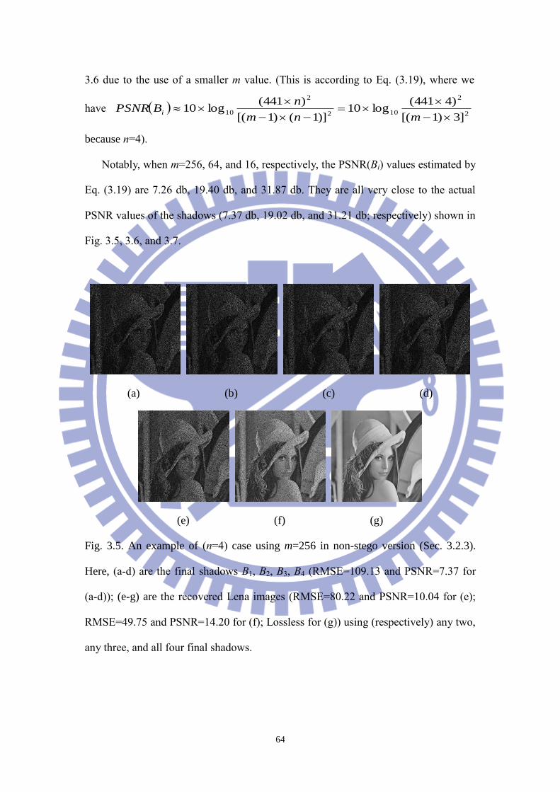
64
3.6 due to the use of a smaller m value. (This is according to Eq. (3.19), where we
have 2
2
102
2
10]3)1[(
)4441(log10
)]1()1[(
)441(log10
mnm
nBPSNR i
because n=4).
Notably, when m=256, 64, and 16, respectively, the PSNR(Bi) values estimated by
Eq. (3.19) are 7.26 db, 19.40 db, and 31.87 db. They are all very close to the actual
PSNR values of the shadows (7.37 db, 19.02 db, and 31.21 db; respectively) shown in
Fig. 3.5, 3.6, and 3.7.
(a) (b) (c) (d)
(e) (f) (g)
Fig. 3.5. An example of (n=4) case using m=256 in non-stego version (Sec. 3.2.3).
Here, (a-d) are the final shadows B1, B2, B3, B4 (RMSE=109.13 and PSNR=7.37 for
(a-d)); (e-g) are the recovered Lena images (RMSE=80.22 and PSNR=10.04 for (e);
RMSE=49.75 and PSNR=14.20 for (f); Lossless for (g)) using (respectively) any two,
any three, and all four final shadows.

65
(a) (b) (c) (d)
(e) (f) (g)
Fig. 3.6. An example of (n=4) case using m=64 in non-stego version (Sec. 3.2.3). Here,
(a-d) are the final shadows B1, B2, B3, B4 (RMSE=28.54 and PSNR=19.02 for (a-d));
(e-g) are the recovered Lena images (RMSE=21.07 and PSNR=21.66 for (e);
RMSE=13.10 and PSNR=25.79 for (f); Lossless for (g)) using (respectively) any two,
any three, and all four final shadows.
(a) (b) (c) (d)
(e) (f) (g)

66
Fig. 3.7. An example of (n=4) case using m=16 in non-stego version (Sec. 3.2.3). Here,
(a-d) are the final shadows B1, B2, B3, B4 (RMSE=7.01 and PSNR=31.21 for (a-d));
(e-g) are the recovered Lena images (RMSE=5.21 and PSNR=33.79 for (e);
RMSE=3.28 and PSNR=37.81 for (f); Lossless for (g)) using (respectively) any two,
any three, and all four final shadows.
(a) (b)
(c) (d)
(e) (f) (g)
Fig. 3.8. An example of (n=4) case using m=32 in stego version (Sec. 3.2.5). Here,
(a-d) are the final stego-shadows B1, B2, B3, and B4; (e-g) are the progressively
recovered Lena images using, respectively, “any” two, “any” three, and all four final

67
shadows. PSNR=26.66 for (a-d); PSNR=10.04 for (e); PSNR=14.21 for (f); and (g) is
lossless.
(a) (b)
(c)
Fig. 3.9. Comparing the stego-shadows in two stego methods for (n=4) case. The
hidden image is Lena (Fig. 3.3(a)) and host image is Jet (Fig. 3.4(a)). Here, (a) is one
of the four stego-shadows with PSNR=26.66 db in our stego version (when m=32); (b)
is one of the four stego-shadows with PSNR=31.26 db in our stego version (when
m=16); (c) is one of the four stego-shadow with PSNR=10.02 in Fang‟s method (Sec.
3.1). Note that our stego size is only 1.6 times (in (a)) or 2 times (in (b)) larger than
original Jet image‟s size, whereas Fang‟s stego size is 4 times larger than original Jet.

68
3.3.2 Comparisons
This sub-section gives a comparison with related researches of other people [3-7, 9,
18-22, 51]. From Table 3.3, we can see that the proposed method owns all these four
advantages: user-friendly, progressive, economical-size, and lossless reconstruction
(when all n shadows are available).
Table 3.3 Comparisons with reported image sharing methods [3-7, 9, 18-22, 51].
Methods Friendly
shadows
Progressive
decoding
Non-expansion in
size of shadows
(n, n) lossless
recovery(1)
Wang and Su [3] x(2)
x yes (3)
yes
Wang et al. [18] x x yes yes
Lin and Tsai [4] x x x yes
Lin and Lin [5] x yes x x
Thien and Lin [7]
yes
(uncontrollable
quality)
x yes x
Fang [19]
yes
(uncontrollable
quality)
yes x yes
Chen and Lin [9] x yes yes yes
Hung et al. [20] x yes yes x
Jin et al. [21] x yes x yes
Fang and Lin [22] x yes x yes
Thien and Lin [6] x x yes yes
Fang and Lin [51] x x x yes
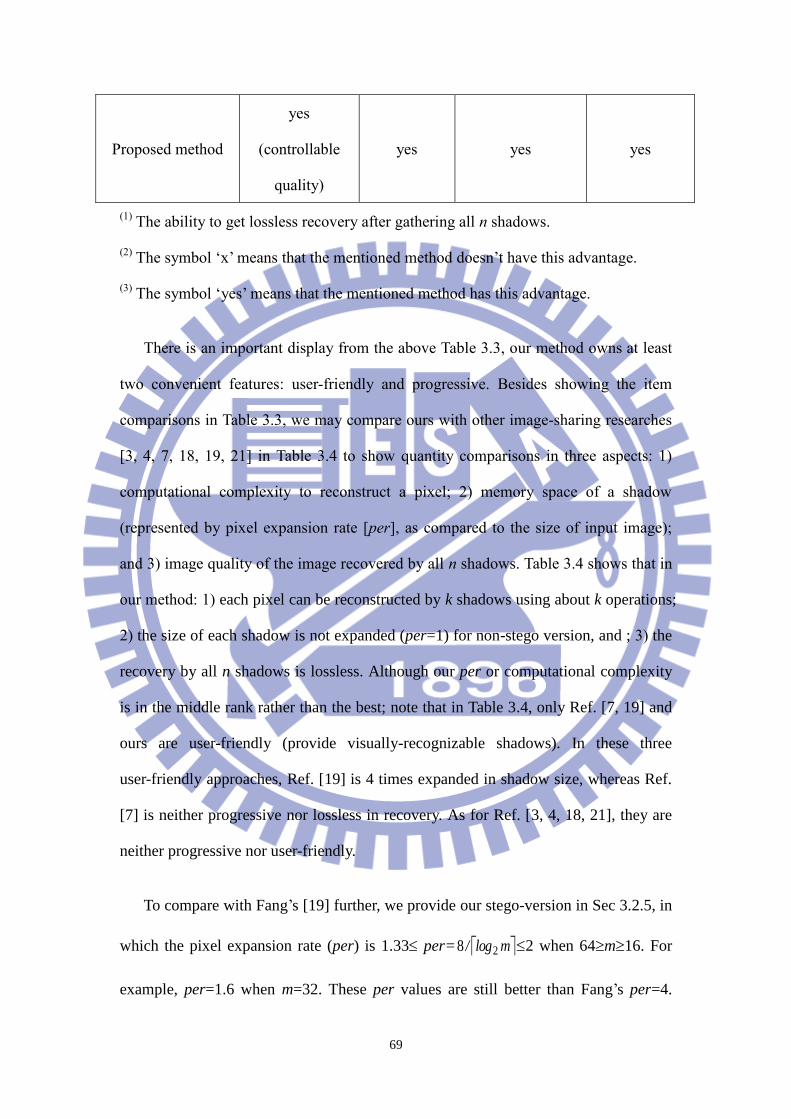
69
Proposed method
yes
(controllable
quality)
yes yes yes
(1) The ability to get lossless recovery after gathering all n shadows.
(2) The symbol „x‟ means that the mentioned method doesn‟t have this advantage.
(3) The symbol „yes‟ means that the mentioned method has this advantage.
There is an important display from the above Table 3.3, our method owns at least
two convenient features: user-friendly and progressive. Besides showing the item
comparisons in Table 3.3, we may compare ours with other image-sharing researches
[3, 4, 7, 18, 19, 21] in Table 3.4 to show quantity comparisons in three aspects: 1)
computational complexity to reconstruct a pixel; 2) memory space of a shadow
(represented by pixel expansion rate [per], as compared to the size of input image);
and 3) image quality of the image recovered by all n shadows. Table 3.4 shows that in
our method: 1) each pixel can be reconstructed by k shadows using about k operations;
2) the size of each shadow is not expanded (per=1) for non-stego version, and ; 3) the
recovery by all n shadows is lossless. Although our per or computational complexity
is in the middle rank rather than the best; note that in Table 3.4, only Ref. [7, 19] and
ours are user-friendly (provide visually-recognizable shadows). In these three
user-friendly approaches, Ref. [19] is 4 times expanded in shadow size, whereas Ref.
[7] is neither progressive nor lossless in recovery. As for Ref. [3, 4, 18, 21], they are
neither progressive nor user-friendly.
To compare with Fang‟s [19] further, we provide our stego-version in Sec 3.2.5, in
which the pixel expansion rate (per) is 1.33 per= mlog/ 28 2 when 64m16. For
example, per=1.6 when m=32. These per values are still better than Fang‟s per=4.

70
(Hence, no matter it is stego version or not, our per is better than Fang‟s.) Moreover,
our stego shadow‟s image quality is also better than Fang‟s (see Fig. 3.9, our
Jet-stego-shadows are with PSNR=26.66 db for m=32 and 31.26 db for m=16, both
are better than Fang‟s 10.02 db).
Table 3.4. Quantity comparisons with reported image sharing methods [3, 4, 7, 18, 19,
21].
Methods Computational
complexity(1)
Memory
size(2)
for
each shadow
Recovered
quality(3)
Wang and Su [3] O(log
2k) (Math
operations(4)
)
per (1/k)×
60% (1/n)×
60%
Lossless
Wang et al. [18] k1 (XOR
operations) per = 1 Lossless
Lin and Tsai [4] O(k×per) (OR-like
operations)
per ≧ 2 Lossless
Thien and Lin
[7] (visually
recognizable
shadows)
O(log2k) (Math
operations)
per 1/k
1/n
Lena‟s PSNR = 37.98
Jet‟s PSNR = 39.93
Baboon‟s PSNR = 35.33
Fang [19]
(visually
recognizable
shadows and
4×(k1) (OR-like
operations) per = 4 Lossless

71
progressive)
Jin et al. [21]
(progressive)
4×(k1) (XOR
operations) per = 4 Lossless
Our Sec 3.2.3
(visually
recognizable
shadows and
progressive)
k additions; 2 Mod
operations; 1
subtraction
per = 1 Lossless
Our stego
version Sec 3.2.5
(visually
recognizable
shadows and
progressive)
(k1) additions; 2
Mod operations; 1
attaching of a short
binary number to the
other to get an 8-bit
number
1.33 per=
mlog/ 28 2
when
64m16
Lossless
(1) Operations needed to recover one secret pixel by k shadows in (k, n) system.
(2) The pixel expansion rate (per) of each shadow, as compared to the input secret
image.
(3) The secret image recovered by all shadows.
(4) Math operations: +,-,×,÷.
3.4 Summary
Many researches in image sharing had been reported, usually traditional
approaches: polynomial sharing or visual cryptography. In this chapter, based on
modulus operations, we successfully designed a novel image sharing method with
user-friendly shadows and progressive decoding. According to the experimental

72
results and comparisons in Sec. 3.3, besides being 1) user-friendly ; 2) progressive; 3)
each pixel is reconstructed by k shadows quickly with about k operations; 4) the
recovery is lossless after collecting all n shadows; the proposed method also owns
following features: 5) the non-stego shadows‟ image quality can be controlled by the
parameter value m using Eq. (3.20); 6) each shadow is not expanded in non-stego
version (Sec. 3.2.3), and is only 1.33per= mlog/ 28 1.6 times larger than original
secret image if we restrict 64m32 in the stego version (Sec. 3.2.5); 7) the stego
shadows have quality much better than Fang‟s shadows (Fig. 3.9).

73
Chapter 4
Multi-Images Sharing with Economical Shadows
and Fast Decoding
In this chapter, we proposed a novel secret sharing scheme for multiple images
based on modulus (MOD) and exclusive-OR (XOR) operations to simultaneously
achieve these two advantages: (1) O/I size ratio is very close to 1, and (2) only
constant computational operations are needed to reconstruct each secret pixel. Notably,
when multiple input images are shared by a scheme, the “O/I size ratio” in this
dissertation denotes the ratio of total size of output shadows divided by total size of
input images. The proposed method generates n extremely noise-like shadows for n
given grayscale (binary/color) secret images (notably, all n given images have the
same size), so that each shadow‟s size is identical to the given images‟. In other words,
our O/I size ratio is 1; therefore, our method will not need extra space in
images-database, when we use the generated shadows to replace original secret
images. Furthermore, after gathering all n shadows, the lossless decoding process only
uses one XOR, one MOD, one addition (ADD) and one subtraction (SUB) operations
(symbolized as “⊕”, “Mod”, “+” and “-” in this dissertation) to reconstruct each
pixel‟s 8-bits value of given secret images, whatever the value of n is. Therefore, no
matter how many secret images are used in our method, the CPU time in decoding
each secret image will not increase as the number of secret images increase. Hence,
the proposed method is not only economical in storage space of shadows but also fast
in decoding of secret images.

74
The remaining portion of the chapter is organized as follows. Section 4.1
describes two basic tools based on MOD and XOR operations respectively; and these
tools will be used in the proposed method. Section 4.2 presents the proposed method.
Section 4.3 gives security analysis. Experimental result and comparisons are in
Section 4.4. Finally, the summary is in Section 4.5.
4.1 Two Basic Tools Used in the Proposed Scheme
To achieve the two advantages (lower O/I size ratio and fewer decoding
operations) mentioned in Sec. 1.1, two basic tools will be used in the proposed
method. The first is the “MOD-based (2, 2) secret sharing tool” in Sec. 4.1.1, which
can make our O/I size ratio be 1. The other is the “XOR-based (n, n) shadows
combination tool” in Sec. 4.1.2, which can make our (n, n) scheme only need constant
operations to decode each secret pixel, no matter how large the value of n is.
4.1.1 MOD-based (2, 2) secret sharing tool
Thien and Lin proposed a modified version [6] of Shamir‟s (k, n)-threshold PSS
approach [1] to reduce the size of shadows. They use polynomials to share a secret
image A among n shadows nBBB ,...,, 21; and each of them is k times smaller than A in
size. A cannot be revealed unless k of the n shadows are gathered. In their encoding,
to transform a sector { 110 ,...,, kaaa } formed of k secret pixel values of A into n
shadow pixel values {nbbb ,...,, 21
} (where each biBi), they use a prime number
p=251 to create a polynomial
)...()( 1
110
k
k xaxaaxq Mod p (4.1)
of degree k-1. Then evaluate ).(,),2(),1( 21 nqbqbqb n Later, using any k of

75
the n produced pairs n
iibi1
),(
, people can recover all k coefficients 110 ,...,, kaaa in
q(x) by constructing the interpolation polynomial.
To let our method have shadows with small size, we apply [6]. More specifically,
apply [6] in a special manner (k=2, n=2). We call this (2, 2) scheme as “MOD-based
(2, 2) secret sharing tool”. The tool is described as follows:
Sharing Phase: (see “(2, 2)-MOD-SS” in left-top part of Fig. 4.1)
Step 1. Use a prime number key to generate a permutation sequence to permute all
pixels‟ positions of the given grayscale image A. Then attach the key in the
permuted image A~
.
Step 2. Sequentially read in gray values {pi} of A~
and then store in array E
according to the rules:
Step 2.1. If pi<250, then store pi in E.
Step 2.2. If pi≧250, then split pi into two values 250 and (pi-250). Store
these two values in E (first 250, then pi-250).
Step 3. Sequentially grab two not-shared-yet elements 0a and 1a of E. Use the
grabbed (0a , 1a ) to evaluate
)()1( 101 aaqb Mod 251 , (4.2)
)2()2( 102 aaqb Mod 251. (4.3)
Then attach 1b to shadow B1, and attach 2b to shadow B2.
Step 4. Repeat Step 3 until all elements of the array E are processed.
Notably, Step 2.2 is to handle the gray values larger than 250 (see [6]), which
seldom happens for most natural images. Therefore, the size of E, which equals to the
total size of B1 and B2, is very close to size of A. In other words, each of the created B1

76
and B2 is about two times smaller than A in size.
Reveal Phase: (see “Reveal of (2, 2)-MOD-SS” in bottom part of Fig. 4.2)
Step 1. Take the first non-used pixel from each of the two shadows B1 and B2. Call the
two values as ( 1b , 2b ).
Step 2. Use these two values ( 1b , 2b ) to recover the two coefficients (0a , 1a ) in Eq.
(4.2-4.3) by
)251( 121 bba Mod 251, (4.4)
)251( 110 aba Mod 251. (4.5)
The recovered (0a , 1a ) are the two corresponding values in E.
Step 3. Repeat Steps 1-2 until all values of the two shadows B1 and B2 are processed.
Step 4. Sequentially grab an element pi of E, then do:
Sub-step 4.1. If pi<250, then store pi in A~
. Now, delete pi from E because the
information contained in pi has been used.
Sub-step 4.2. If pi=250, then read in pi+1 immediately. Then store the single
value (250+pi+1) in A~
. Now, delete both pi and pi+1 from E because the
information in pi and pi+1 have both been used.
Step 5. Extract the prime number key from A~
and apply the inverse-permutation
operation to the permuted image A~
to get back to the secret image A.
In the reveal algorithm above, only three operations (one SUB, one ADD and one
MOD) are needed in Eq. (4.4) or Eq. (4.5) to reconstruct each secret pixel of A~
.
Because usually there are only a few pixels in A (and hence, in A~
) whose gray values
are above 250, the ADD operation in Sub-step 4.2 seldom occurs. Also, for each pixel,
Step 5 uses one mapping operation (indexing) rather than computational operation.

77
4.1.2 XOR-based (n, n) shadows combination tool
Once all given n secret images nAAA ,...,, 21 are processed by MOD-based (2, 2)
secret sharing tool described in Sec. 4.1.1, each secret image iA ( ni 1 )
generates two half-size temporary shadows 1,iB and 2,iB . To avoid any secret
leaking when collecting less than n final shadows, we use the following steps of
Combination Phase to form the final shadowiC .
Combination Phase: (see right-top and bottom parts of Fig. 4.1)
Step 1. (Size-synchronization.) If some shadows jiB , ( ni 1 and 21 j ) have
distinct size due to the existence of pixels whose gray values are in 251-255 in
some images iA , then add suitable number of dummy pixels in all shadows to
make all shadows jiB , have the same size as the one with the largest size.
Step 2. (Stacking.) Take the first not-yet-processed pixel 1,ib from each shadow 1,iB
( ni 1 ). Then evaluate the corresponding pixel *b for a new image *B
by
1,1,21,1* nbbbb . (4.6)
After all pixels of all 1,iB are processed, the generation of image *B is done,
and its size is the same as 1,iB (and 2,iB , too).
Step 3. (Shifting 2,iB to 3,iB .) Take next not-yet-processed pixel 2,ib from each
shadow 2,iB ( ni 1 ), and, at the same pixel position, take the
corresponding pixel *b *B . Then create the corresponding pixel value 3,ib

78
of a new image 3,iB by
*2,3, bbb ii ( ni 1 ). (4.7)
After all pixels in all 2,iB are processed, all n images 3,iB are generated.
Notably, each 3,iB is as large as each 2,iB .
Step 4. (Physically gluing.) For ni 1 , physically combine each pair of 1,iB and
3,iB to generate their final shadowiC =( 1,iB ; 3,iB ) . Because 1,iB and 3,iB are
both about two times smaller thaniA , each
iC is about as large asiA .
When all n final shadows nCCC ,...,, 21 are gathered, we can reconstruct all 1,iB
and 2,iB ( ni 1 ) by using the following steps of Decomposing Phase whose
computation is very low.
Decomposition Phase: (see top part of Fig. 4.2)
Step 1. For ni 1 , physically separate each iC =( 1,iB ; 3,iB ) into two halves to
get 1,iB (front half) and 3,iB (rear half).
Step 2. Take next not-yet-processed pixel 1,ib from each 1,iB ( ni 1 ). Then
evaluate the corresponding pixel *b in the image *B by Eq. (4.6). After all
pixels of all 1,iB are processed, the image *B is generated.
Step 3. Take next not-yet-processed pixel 3,ib from each 3,iB ( ni 1 ), and, at the
same pixel position, take the corresponding pixel *b from *B . Then
evaluate the corresponding pixel 2,ib for each image 2,iB by
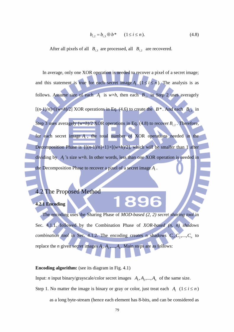
79
*3,2, bbb ii ( ni 1 ). (4.8)
After all pixels of all 3,iB are processed, all 2,iB are recovered.
In average, only one XOR operation is needed to recover a pixel of a secret image;
and this statement is true for each secret imageiA ( ni 1 ). The analysis is as
follows. Assume size of each iA is w×h, then each 1,iB in Step 2 uses averagely
[(n-1)/n]×[(w×h)/2] XOR operations in Eq. (4.6) to create the *B . And each 3,iB in
Step 3 uses averagely (w×h)/2 XOR operations in Eq. (4.8) to recover 2,iB . Therefore,
for each secret imageiA , the total number of XOR operations needed in the
Decomposition Phase is {[(n-1)/n]+1}×[(w×h)/2], which will be smaller than 1 after
dividing by iA ‟s size w×h. In other words, less than one XOR operation is needed in
the Decomposition Phase to recover a pixel of a secret imageiA .
4.2 The Proposed Method
4.2.1 Encoding
The encoding uses the Sharing Phase of MOD-based (2, 2) secret sharing tool in
Sec. 4.1.1, followed by the Combination Phase of XOR-based (n, n) shadows
combination tool in Sec. 4.1.2. The encoding creates n shadows nCCC ,...,, 21 to
replace the n given secret images nAAA ,...,, 21 . Main steps are as follows:
Encoding algorithm: (see its diagram in Fig. 4.1)
Input: n input binary/grayscale/color secret images nAAA ,...,, 21 of the same size.
Step 1. No matter the image is binary or gray or color, just treat each iA ( ni 1 )
as a long byte-stream (hence each element has 8-bits, and can be considered as
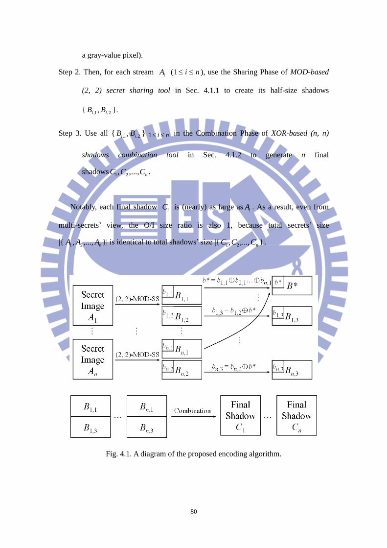
80
a gray-value pixel).
Step 2. Then, for each stream iA ( ni 1 ), use the Sharing Phase of MOD-based
(2, 2) secret sharing tool in Sec. 4.1.1 to create its half-size shadows
{ 1,iB , 2,iB }.
Step 3. Use all { 1,iB , 2,iB } ni 1 in the Combination Phase of XOR-based (n, n)
shadows combination tool in Sec. 4.1.2 to generate n final
shadowsnCCC ,...,, 21.
Notably, each final shadow iC is (nearly) as large as
iA . As a result, even from
multi-secrets‟ view, the O/I size ratio is also 1, because total secrets‟ size
|{ nAAA ,...,, 21}| is identical to total shadows‟ size |{
nCCC ,...,, 21}|.
Fig. 4.1. A diagram of the proposed encoding algorithm.

81
4.2.2 Decoding
To recover the n secret images nAAA ,...,, 21
from the n final shadows
nCCC ,...,, 21, the decoding uses the Decomposition Phase of the XOR-based (n, n)
shadows combination tool in Sec. 4.1.2, followed by the Reveal Phase of the
MOD-based (2, 2) secret sharing tool in Sec. 4.1.1. Main steps are as follows:
Decoding algorithm: (see its diagram in Fig. 4.2)
Step 1. Use the Decomposition Phase of the XOR-based (n, n) shadows combination
tool in Sec. 4.1.2 to reconstruct the half-size images { 1,iB ; 2,iB } ni 1 from
the n final shadows {nCCC ,...,, 21}.
Step 2. For each pair { 1,iB ; 2,iB }, where ni 1 , use the Reveal Phase of MOD-based
(2, 2) secret sharing tool in Sec. 4.1.1 to recover the secret image iA from
{ 1,iB ; 2,iB }.
Step 3. If the original secret images are not gray-valued, then transform all n 8-bits
images nAAA ,...,, 21 to their binary/color equivalent.
In average, the decoding only needs one XOR, one MOD, one ADD and one SUB
operations (all are between bytes) to reconstruct each 1-byte (8-bits) pixel value of a
secret image. More specifically, in Step 1 of decoding, one XOR operation is needed
to recover a 1-byte pixel value of 2,iB for the Decomposition Phase of the
XOR-based (n, n) shadows combination tool. In Step 2, one MOD, one ADD and one
SUB operations are needed to recover a 1-byte pixel value of iA in the Reveal Phase
of the MOD-based (2, 2) secret sharing tool.

82
Fig. 4.2. A diagram of the proposed decoding algorithm.
4.3 Security Analysis
Assume that only n-1 final shadows are available, and a shadow jC is missing.
Then, people cannot obtain *B created by 1,1,21,1* nbbbb in Eq. (4.6),
due to the lack of the 1,jb which is in the front half of jC . Without *B , people
cannot reconstruct 2,2,22,1 ,...,, nBBB defined by *3,2, bbb ii ( ni 1 ) in Eq.
(4.8). As a result, no secret image iA can be recovered (see the Reveal Phase of
MOD-based (2, 2) secret sharing tool in Sec. 4.1.1) due to absence of all 2,iB
( ni 1 ).
Below we discuss the probability of obtaining some right secret images iA
through guessing. Without the loss of generality, assume that a betrayal party of n-1
participants gathers their n-1 final shadows 121 ,...,, nCCC , and try to recover some of
the n secret images, without the cooperation of the missing shadow nC . From Eq. (4.6)

83
and (4.8) , we have
1,1,21,13,3,2, * niii bbbbbbb ( ni 1 ). (4.9)
Because of the lack of nC =[ 1,nB ; 3,nB ], for each pixel 1,nb in 1,nB , the betrayal party
will have to guess a value, and then they use this guessing value to get a set of n-1
pixels‟ values 2,12,22,1 ,...,, nbbb in 2,12,22,1 ,...,, nBBB respectively at the same pixel
position (there is no 2,nb value in 2,nB due to the lack of 3,nb ). Then the 2×(n-1)
secret pixels in 121 ,...,, nAAA can be reconstructed by using 1,ib and 2,ib
( 11 ni ) in the Reveal Phase of MOD-based (2, 2) secret sharing tool in Sec.
4.1.1. The above is just to reconstruct two pixels in each iA ( 11 ni ). This
value-guessing of one pixel, like 1,nb , will repeat (w×h)/2 times if the size of each iA
is w×h (then, size of 1,nB is 0.5×w×h).
From the description above, we can evaluate the probability of obtaining some
right grayscale images iA of size w×h as follows:
22 )251
1()
range values
1(yProbabilit
hwhw
which is 31453010131072)251
1(2/512512)
251
1(
if each image size is 512512 .
Here, 251
1
range values
1 is the probability to guess successfully a pixel‟s value
whose range is from 0 to 250; 2
hw is the number of pixels in 1,nB . In fact, for each
secret image iA ( ni 1 ) in the encoding process (as we did in Step 1 of the
Sharing Phase of MOD-based (2, 2) secret sharing tool in Sec. 4.1.1), we already use
a prime number as a key (a seed) of a random number generator to rearrange all
pixels‟ positions of iA . Even if many pixels‟ values in 1,nB are guessed successfully,

84
in Step 4 of Reveal Phase of MOD-based (2, 2) secret sharing tool in Sec. 4.1.1, the
recovered imagesiA
~ ( 11 ni ) are still extremely noise-like. Therefore, the
security guardian is of double levels.
4.4 Experimental Result and Comparisons
4.4.1 Experimental Result
In the experiment here, n=5 and the n input images {521 ,...,, AAA } are the
512512 grayscale images {Jet, Lena, Pepper, Scene and Baboon} shown in Fig.
4.3(a-e). The n=5 final shadows {521 ,...,, CCC } generated in Sec. 4.2.1 are shown in
Fig. 4.4(a-e), and each shadow is as large as each input image. Fig. 4.5(a-e) shows
five error-free recovered images 521 ,...,, AAA (Jet, Lena, Pepper, Scene and Baboon)
in Sec. 4.2.2 using all n=5 final shadows521 ,...,, CCC . If we only get four shadows,
saying, the 421 ,...,, CCC in Fig. 4.4(a-d); and then guess the pixel values of images
1,5B and 2,5B ; then the five recovered images of 521 ,...,, AAA are the extremely
noise-like images shown in Fig. 4.6. In addition, to show our constant decoding-time
property in the retrieval, we also record in Fig. 4.7 the actual CPU time taken in
decoding. The computer used is an IBM laptop with an Intel Pentium 1.70GHz CPU.
From Fig. 4.7, which deals with n images for 102 n , it can be seen that our
decoding time for each one of the n secret image really does not vary as the value of n
varies.

85
(a) (b)
(c) (d) (e)
Fig. 4.3. The five input grayscale images in the n=5 case.
(a) (b)

86
(c) (d) (e)
Fig. 4.4. The five generated noise-like shadows {521 ,...,, CCC } in the n=5 case.
(a) (b)
(c) (d) (e)
Fig. 4.5. The five error-free images recovered by using all five shadows (Fig. 4.4) in
the n=5 case.

87
(a) (b)
(c) (d) (e)
Fig. 4.6. The n=5 images54321 ,,,, AAAAA recovered by using only four shadows
4321 ,,, CCCC (Fig. 4.4 (a-d)) and two guessed images 1,5B and 2,5B in the n=5
case.
0
10
20
30
2 3 4 5 6 7 8 9 10
n
millisecond
n 2 3 4 5 6 7 8 9 10
millisecond 15 ms 15 ms 15 ms 15 ms 15 ms 15 ms 15 ms 15 ms 15 ms

88
Fig. 4.7. The CPU time (milliseconds) for decoding 512×512 pixels of one image in
our (n, n) systems. (So the CPU time for decoding 512×512 pixels of all n images are
15n milliseconds.)
4.4.2 Comparisons
Table 4.1 compares between our method and other multi-secrets schemes [23-26]
in terms of two quantifiable measures: 1) O/I size ratio and 2) decoding computational
complexity. For comparison, the same conditions hold for each scheme; they are: (1)
there are n secret images; (2) every recovered image must be lossless; (3) The
computer versions of VC schemes [24, 25] are implemented using OR-like operation
to simulate the stacking action of transparencies. From Table 4.1, we can see that our
method not only keeps O/I size ratio as small as 1, but also needs only constant
decoding operations to reconstruct a secret pixel. Other schemes either have O/I size
ratio larger than 1, or need non-constant decoding complexity to reconstruct a secret
pixel.
Table 4.1. O/I size ratio and decoding complexity.
Schemes O/I size ratio(1)
(smaller is better)
Decoding complexity(2)
(smaller is better)
Feng et al. [23] 1 ~ 2 O(log2k) (Math operations)
(3)
Shyu et al. [24] 4 2×n (OR-like operations)
Feng et al. [25] 6 3×n (OR-like operations)
Alvarez et al. [26] (n+1)/n 1 (MOD operation) and
O(n) (Math operations(4)
)

89
Our scheme 1 1 XOR, 1 MOD, 1 ADD
, and 1 SUB operations
(1) Total size of shadows divided by total size of input images.
(2) Complexity to decode a pixel of a secret image.
(3) k is a user-specified threshold value, it can depend on n or not; e.g. k=0.5n or k=3.
(4) Math operations: +, -, ×, ÷.
4.5 Summary
In this chapter, a novel lossless sharing scheme for multiple secret images is
designed using MOD and XOR operations. Our advantages are: i) the total size of the
n given secret images are the same as the total size of the n final shadows (hence our
O/I size ratio is 1); ii) we only needs one XOR, one MOD, one ADD and one SUB
(all are byte-to-byte) operations to get a lossless recovery of each secret pixel‟s 8-bits
value for the given binary/grayscale/color images (hence our decoding computational
complexity for each pixel is a constant and independent of n).

90
Chapter 5
Conclusions and Future Works
5.1 Conclusions
In this dissertation, we have proposed three methods to improve and extend
image sharing techniques. The first is a Boolean-based missing-allowable (k, n)
scheme which is fast and with reasonable size of shadows. The second is a
modulus-operations-based sharing scheme equipped with user-friendly shadows and
progressive decoding simultaneously. The last is a scheme that shares multiple images
by using both Boolean and modulus operations; it is with economical shadow size and
low decoding computational load.
In order to improve secret sharing for single image in storage space and
computational complexity, we have designed successfully an economical and fast
scheme based on Boolean (XOR) operations in Chapter 2. In that method, the pixel
expansion rate (per) of the generated shadows is between 0 and 2, hence the storage
space of shadows is reasonable. Moreover, it is close to 0 when the value if k is large
and close to the value of n in a (k, n) scheme, e.g. per=2/n in all (n, n) schemes. In
computational complexity, the scheme only uses three 1-bit/8-bit/24-bit XOR
operations per secret pixel to recover the given binary/grayscale/color image. Besides,
unlike some probabilistic approaches, our recovered image is lossless. Our scheme is
missing-allowable because it is a (k, n)-threshold scheme, which requires only k out of
the n shadows appear in the recovery meeting.
In Chapter 3, besides being with user-friendly shadows and progressive decoding,
our method also owns other advantages: (1) the non-stego shadows‟ image quality can

91
be controlled by a parameter value; (2) each shadow is not expanded in the non-stego
version (Sec. 3.2.3), and it is at most only 1.6 times larger than original secret image
in the stego version (Sec. 3.2.5); (3) each pixel can be reconstructed by k shadows
quickly with linear computational complexity O(k); and (4) the recovery is lossless
after collecting all n shadows.
In order to deal with multiple images, based on Boolean (XOR) and modulus
operations, we have designed successfully a multi-images scheme in Chapter 4 that
saves storage space of shadows and reduces decoding computational complexity. In
the proposed method, the total size of the generated shadows is identical to that of the
given secret images. Therefore, our method will not need extra space in
images-database to store the generated shadows that replaces the original secret
images. Furthermore, after gathering all n shadows, the lossless decoding process only
uses constant operations to reconstruct each pixel of each given secret image,
whatever the n is. Hence no matter how many secret images are used in our method,
the CPU time in decoding each secret image will not increase as the number of secret
images increases.
5.2 Future Works
In Chapters 2 and 3, the two proposed methods only work for single image: they
can not deal with two or more images simultaneously in one sharing process.
However, simultaneous dealing with multiple images is very common in today‟s
business. Several studies in sharing of multiple images had been reported [23-29].
Unfortunately, these reported methods either have big-size shadow images [24-25, 27]
or huge stego images [23, 29]) or need an extra shadow image called public shadow
[26]. Moreover, for decoding, the amount of operations linearly increases as the

92
number of secret images [26] or gathered shadows [23] increases. In Chapter 4, we
had successfully designed an improved multiple-images method, emphasizing the
reduction of both storage space and computational complexity. Our multi-images
scheme can share n given secret images and generate n non-expanded shadow images.
This novel scheme only needs a few computational operations in the recovery of each
secret pixel; whatever the value of n is.
Although our method is better than other multi-images schemes in O/I size ratio
and decoding time; the multi-images schemes [23-26] have advantages of their own: 1)
Feng et al.‟s [23] uses generalized access structures to achieve higher flexibility; 2) if
the shadows are printed in transparencies, then the VC schemes [24-25] can also
reveal images by doing physical stacking of transparencies (although true-color
images will be very hard for VC to retrieve error-freely by stacking transparencies); 3)
Alvarez et al.‟s method [26] can process n given secret images of non-equal sizes.
To improve our multi-images sharing scheme in the future, the above three
advantages of [23-26] will be the main guideline of ours. Also, besides the space and
time efficiency that we already achieved herein; in the future, we hope to add to our
multi-images scheme some other features, such as the missing-allowable property,
user-friendly shadows, and progressive decoding.

93
References
[1] A. Shamir, “How to share a secret,” Communications of the ACM, Vol. 22, No. 11,
pp. 612613, 1979.
[2] M. Naor and A. Shamir, “Visual cryptography,” Advances in Cryptography -
EUROCRYPT’94; Lecture Notes in Computer Science, Vol. 950, pp. 112, 1995.
[3] R. Z. Wang and C. H. Su, “Secret image sharing with smaller shadow images,”
Pattern Recognition Letters, Vol. 27, pp. 551-555, 2006.
[4] C. C. Lin and W. H. Tsai, “Visual cryptography for gray-level images by dithering
techniques,” Pattern Recognition Letters, Vol. 24, pp. 349-358, 2003.
[5] S. J. Lin and J. C. Lin, “VCPSS: A two-in-one two-decoding-options image
sharing method combining visual cryptography (VC) and polynomial-style
sharing (PSS) approaches,” Pattern Recognition, Vol. 40, pp. 3652-3666, 2007.
[6] C. C. Thien and J. C. Lin, “Secret image sharing,” Computers and Graphics, Vol.
26, No. 5, pp. 765-770, 2002.
[7] C. C. Thien and J. C. Lin, “An image-sharing method with user-friendly shadow
images,” IEEE Trans. Circuits & Systems for Video Technol., Vol. 13, No. 12, pp.
1161-1169, 2003.
[8] Y. S. Wu, C. C. Thien and J. C. Lin, “Sharing and hiding secret images with size
constraint,” Pattern Recognition, Vol. 37, pp. 1377-1385, 2004.
[9] S. K. Chen and J. C. Lin, “Fault-tolerant and progressive transmission of images,”
Pattern Recognition, Vol. 38, pp. 2466-2471, 2005.
[10] C. N. Yang and T. S. Chen, “Aspect ratio invariant visual secret sharing schemes
with minimum pixel expansion,” Pattern Recognition Letters, Vol. 26, pp.
193-206, 2005.
[11] C. N. Yang and T. S. Chen, “Extended visual secret sharing schemes: improving

94
the shadow image quality,” International Journal of Pattern Recognition and
Artificial Intelligence, Vol. 21, pp. 879-898, 2007.
[12] Y. C. Hou, “Visual cryptography for color images,” Pattern Recognition, Vol. 36,
pp. 1619-1629, 2003.
[13] R. Lukac and K. N. Plataniotis, “A color image secret sharing scheme satisfying
the perfect reconstruction property,” IEEE 6th
Workshop on Multimedia signal
Processing, Siena, Italy, September 29-October 1, 2004 (pp. 351-354).
[14] R. Lukac and K. N. Plataniotis, “Color image secret sharing,” IEE Electronics
Letters, Vol. 40, pp. 529-531, 2004.
[15] R. Lukac and K. N. Plataniotis, “Bit-level based secret sharing for image
encryption,” Pattern Recognition, Vol. 38, pp. 767-772, 2005.
[16] C. N. Yang, “New visual secret sharing schemes using probabilistic method,”
Pattern Recognition Letters, Vol. 25, pp. 481-494, 2004.
[17] F. Yi, D. Wang, X. Li and Y. Dai, “Colored probabilistic visual cryptography
scheme with reversing,” Security and Management, pp. 138-141, 2007.
[18] D. Wang, L. Zhang, N. Ma and X. Li, “Two secret sharing schemes based on
Boolean operations,” Pattern Recognition, Vol. 40, pp. 2776-2785, 2007.
[19] W. P. Fang, “Friendly progressive visual secret sharing,” Pattern Recognition,
Vol. 41, pp. 1410-1414, 2008.
[20] K. H. Hung, Y. J. Chang, and J. C. Lin, “Progressive sharing of an image,”
Optical Engineering, Vol. 47, No. 4, pp. 047006-1-047006-14, 2008.
[21] D. Jin, W. Q. Yan, and M. S. Kankanhalli, “Progressive color visual
cryptography,” Journal of Electronic Imaging, Vol. 14, No. 3, pp.
033019-1-033019-13, 2005.
[22] W. P. Fang and J. C. Lin, “Progressive viewing and sharing of sensitive images,”
Pattern Recognition and Image Analysis, Vol. 16, No. 4, pp. 632-636, 2006.

95
[23] J. B. Feng, H. C. Wu, C. S. Tsai and Y. P. Chu, “A new multi-secret images
sharing scheme using Largrange‟s interpolation,” The Journal of Systems and
Software, Vol. 76, pp. 327-339, 2005.
[24] S. J. Shyu, S. Y. Huang, Y. K. Lee, R. Z. Wang and K. Chen, “Sharing multiple
secrets in visual cryptography,” Pattern Recognition, Vol. 40, pp. 3633-3651,
2007.
[25] J. B. Feng, H. C. Wu, C. S. Tsai, Y. F. Chang and Y. P. Chu, “Visual secret
sharing for multiple secrets,” Pattern Recognition, Vol. 41, pp. 3572-3581, 2008.
[26] G. Alvarez, L. H. Encinas and A. M. del Rey, “A multisecret sharing scheme for
color images based on cellular automata,” Information Sciences, Vol. 178, pp.
4382-4395, 2008.
[27] H. C. Wu and C. C. Chang, “Sharing visual multi-secrets using circle shares,”
Computer Standards & Interfaces, Vol. 28, pp. 123-135, 2005.
[28] C. S. Tsai, C. C. Chang and T. S. Chen, “Sharing multiple secrets in digital
images,” The Journal of Systems and Software, Vol. 64, pp. 163-170, 2002.
[29] W. P. Fang and J. C. Lin, “Universal share for the sharing of multiple images,”
Journal of the Chinese Institute of Engineers, Vol. 30, No. 4, pp. 753-757, 2007.
[30] R. Lukac and K. N. Plataniotis, “A cost-effective encryption scheme for color
images,” Real-Time Imaging, Vol. 11, pp. 454-464, 2005.
[31] C. C. Chang, C. C. Lin, C. H. Lin and Y. H. Chen, “A novel secret image sharing
scheme in color images using small shadow images,” Information Sciences, Vol.
178, pp. 2433-2447, 2008.
[32] C. Blundo and A. D. Santis, “Visual cryptography schemes with perfect
reconstruction of black pixels,” Computers and Graphics, Vol. 22, No. 4, pp.
449-455, 1998.
[33] S. J. Shyu, “Efficient visual secret sharing scheme for color images,” Pattern

96
Recognition, Vol. 39, pp. 866-880, 2006.
[34] C. N. Yang and T. S. Chen, “Reduce shadow size in aspect ratio invariant visual
secret sharing schemes using a square block-wise operation,” Pattern Recognition,
Vol. 39, pp. 1300-1314, 2006.
[35] C. Blundo, S. Cimato and A. D. Santis, “Visual cryptography schemes with
optimal pixel expansion,” Theoretical Computer Science, Vol. 369, pp. 169-182,
2006.
[36] Z. Zhou, G. R. Arce and G. D. Crescenzo, “Halftone visual cryptography,” IEEE
Transactions on Image Processing, Vol. 15, No. 8, pp. 2441-2453, 2006.
[37] R. Lukac and K. N. Plataniotis, “Digital image indexing using secret sharing
schemes: a unified framework for single-sensor consumer electronics,” IEEE
Transactions on Consumer Electronics, Vol. 51, No. 3, pp. 908-916, 2005.
[38] D. C. Lou, H. K. Tso and J. L. Liu, “A copyright protection scheme for digital
images using visual cryptography technique,” Computer Standards and Interfaces,
Vol. 29, pp. 125-131, 2007.
[39] C. N. Yang, T. S. Chen, K. H. Yu and C. C. Wang, “Improvements of image
sharing with steganography and authentication,” The Journal of Systems and
Software, Vol. 80, pp. 1070-1076, 2007.
[40] R. Z. Wang and S. J. Shyu, “Scalable secret image sharing,” Signal Processing:
Image Communication, vol. 22. pp. 363-373, 2007.
[41] C. M. Hu and W. G. Tzeng, “Cheating Prevention in Visual Cryptography,” IEEE
Transactions on Image Processing, Vol. 16, No. 1, pp. , 36-45, 2007.
[42] C. C. Chang, Y. P. Hsieh and C. H. Lin, “Sharing secrets in stego images with
authentication,” Pattern Recognition, Vol. 41, pp. 3130-3137, 2008.
[43] C. C. Chang, C. C. Lin, T. H. N. Le and H. B. Le, “Sharing a verifiable secret
image using two shadows,” Pattern Recognition, Vol. 42, pp. 3097-3114, 2009.

97
[44] G. Ateniese, C. Blundo, A. D. Santis and D. R. Stinson, “Visual cryptography for
general access structures,” Information and Computation, Vol. 129, pp. 86-106,
1996.
[45] Y. F. Chen, Y. K. Chan, C. C. Huang, M. H. Tsai and Y. P. Chu, “A multiple-level
visual secret-sharing scheme without image size expansion,” Information Sciences,
Vol. 177, pp. 4696-4710, 2007.
[46] A. M. del Rey, J. P. Mateus and G. R. Sanchez, “A secret sharing scheme based
on cellular automata,” Applied Mathematics and Computation, vol. 170, pp.
1356-1364, 2005.
[47] Z. Eslami, S. H. Razzaghi and J. Z. Ahmadabadi, “Secret image sharing based on
cellular automata and steganography,” Pattern Recognition, Vol. 43, pp. 397-404,
2010.
[48] M. H. Dehkordi and S. Mashhadi, “An efficient threshold verifiable multi-secret
sharing,” Computer Standards and Interfaces, vol. 30, pp. 187-190, 2008.
[49] Y. J. Chang, S. J. Lin and J. C. Lin, “Authentication and cross-recovery for
multiple images,” Journal of Electronic Imaging, Vol. 17, No. 4, pp.
043007-1-043007-12, 2008.
[50] W. P. Fang and J. C. Lin, “Multi-channel secret image transmission with fast
decoding: by using bit-level sharing and economic-size shares,” IJCSNS -
International Journal of Computer Science and Network Security, Vol. 6, No. 5B,
pp. 228-234, 2006.
[51] W. P. Fang and J. C. Lin, “Visual cryptography with extra ability of hiding
confidential data,” Journal of Electronic Imaging, Vol. 15, No. 2, pp.
023020-1-023020-7, 2006.

98
Vita
Kun-Yuan Chao received his B.S. degree in Computer and Information Science
in 1996 from National Chiao Tung University, Taiwan. Then he received his M.S.
degree in Computer Science and Information Engineering in 1999 from National
Taiwan University, Taiwan. He is currently a Ph.D. candidate of the Computer and
Information Science Department, National Chiao Tung University, Taiwan. His recent
research interests include secret image sharing, visual cryptography and image
processing.

99
Publication List of Kun-Yuan Chao
A. Journal papers
Published:
1. Kun-Yuan Chao and Ja-Chin Lin, “Secret Image Sharing: a
Boolean-operations-based Approach Combining Benefits of Polynomial-based
and Fast Approaches,” International Journal of Pattern Recognition and Artificial
Intelligence, Vol. 23, No. 2, pp. 263-285, March 2009. (SCI)
2. Kun-Yuan Chao and Ja-Chin Lin, “User-friendly Image Sharing: a Progressive
Approach Based on Modulus Operations,” Journal of Electronic Imaging, Vol. 18,
No. 3, pp. 033008-1-033008-9, July-September 2009. (SCI)
3. Kun-Yuan Chao, and Ja-Chin Lin, “Fault-tolerant and Non-expanded Visual
Cryptography for Color Images,” WSEAS Trans. on Information Science &
Applications, Issue 11, Vol. 3, pp. 2184-2191, November 2006.
Revised:
4. Kun-Yuan Chao, and Ja-Chin Lin, “Sharing of Multiple Images: an Economic-Size
and Fast-Decoding Approach based on Modulus and Boolean Operations,”
Optical Engineering, November 2009. (SCI)
B. Conference papers
Published:
5. Kun-Yuan Chao, and Ja-Chin Lin, “(2, 3)-threshold Visual Cryptography for Color

100
Images,” Proc. of the 6th WSEAS International Conference on Signal Processing,
Computational Geometry & Artificial Vision, Elounda, Greece, August 21-23,
2006 (pp. 89-94).
6. Kun-Yuan Chao, “A Progressive Visual Sharing Scheme with Multiple Thresholds",
The 21th IPPR Conference on Computer Vision, Graphics and Image Processing
(CVGIP2008), Yilan, Taiwan, R.O.C., August 24-26, 2008 (pp. 129).


![Chapter 1 Introduction - ir.nctu.edu.tw · 2-2-2 Electron Capture and Emission in RTNs Actually, RTN is formed through a series multi-phonon mechanism. Fig 2.3 [1] shows the detailed](https://img.pdfslide.us/doc/110x75/5e8a2645abc8a2101b0a2adc/chapter-1-introduction-irnctuedutw-2-2-2-electron-capture-and-emission-in-rtns.jpg)
![Chapter 1 Introduction - ir.nctu.edu.tw file1960s[1.2], people generally thought that the time of using vacuum tubes was over. Gradually, vacuum tubes were replaced by solid state](https://img.pdfslide.us/doc/110x75/5e1134bf115cee20ee479a74/chapter-1-introduction-irnctuedutw-12-people-generally-thought-that-the.jpg)
![Chapter 1 Introduction - ir.nctu.edu.tw · [TCC 02] and [FWTC 05] should use computer to extracting the secret images. Although the method in [TCC 02] and [FWTC 05] is very convenient](https://img.pdfslide.us/doc/110x75/5f13799b0f3864417347c243/chapter-1-introduction-irnctuedutw-tcc-02-and-fwtc-05-should-use-computer.jpg)