Embed Size (px)
Citation preview
इरिसट IRISET
TB 6 MEASURING INSTRUMENTS
TB 6
MEASURING INSTRUMENTS
INDIAN RAILWAY INSTITUTE OF SIGNAL ENGINEERING & TELECOMMUNICATION,
SECUNDERABAD - 500007
April 2020
The Material Presented in this IRISET Notes is for
guidance only. It does not over rule or alter any of the
Provisions contained in Manuals or Railway Board’s
directives
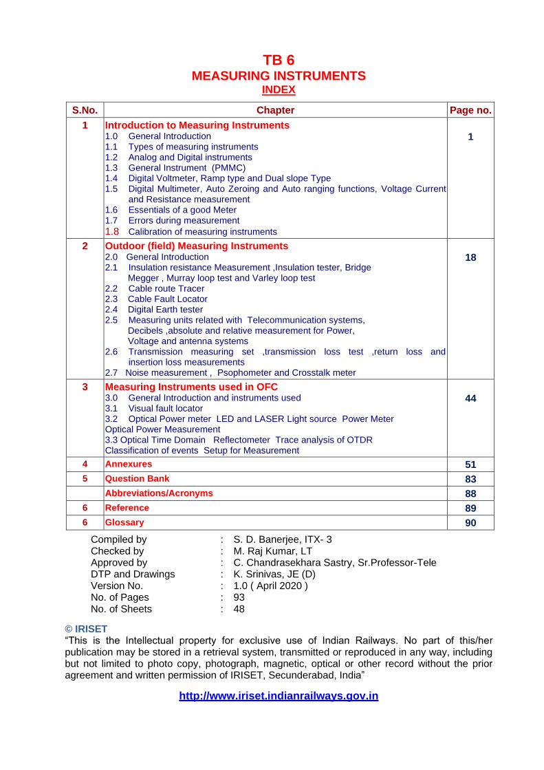
TB 6 MEASURING INSTRUMENTS
INDEX
S.No. Chapter Page no.
1 Introduction to Measuring Instruments 1.0 General Introduction 1.1 Types of measuring instruments 1.2 Analog and Digital instruments 1.3 General Instrument (PMMC) 1.4 Digital Voltmeter, Ramp type and Dual slope Type 1.5 Digital Multimeter, Auto Zeroing and Auto ranging functions, Voltage Current
and Resistance measurement 1.6 Essentials of a good Meter 1.7 Errors during measurement
1.8 Calibration of measuring instruments
1
2 Outdoor (field) Measuring Instruments 2.0 General Introduction 2.1 Insulation resistance Measurement ,Insulation tester, Bridge Megger , Murray loop test and Varley loop test 2.2 Cable route Tracer 2.3 Cable Fault Locator 2.4 Digital Earth tester 2.5 Measuring units related with Telecommunication systems, Decibels ,absolute and relative measurement for Power, Voltage and antenna systems 2.6 Transmission measuring set ,transmission loss test ,return loss and
insertion loss measurements 2.7 Noise measurement , Psophometer and Crosstalk meter
18
3 Measuring Instruments used in OFC 3.0 General Introduction and instruments used 3.1 Visual fault locator 3.2 Optical Power meter LED and LASER Light source Power Meter Optical Power Measurement 3.3 Optical Time Domain Reflectometer Trace analysis of OTDR Classification of events Setup for Measurement
44
4 Annexures 51
5 Question Bank 83
Abbreviations/Acronyms 88
6 Reference 89
6 Glossary 90
Compiled by : S. D. Banerjee, ITX- 3 Checked by : M. Raj Kumar, LT Approved by : C. Chandrasekhara Sastry, Sr.Professor-Tele DTP and Drawings : K. Srinivas, JE (D) Version No. : 1.0 ( April 2020 ) No. of Pages : 93 No. of Sheets : 48
© IRISET “This is the Intellectual property for exclusive use of Indian Railways. No part of this/her publication may be stored in a retrieval system, transmitted or reproduced in any way, including but not limited to photo copy, photograph, magnetic, optical or other record without the prior agreement and written permission of IRISET, Secunderabad, India”
http://www.iriset.indianrailways.gov.in
IRISET 1 TB6 - Measuring instruments
CHAPTER-1
INTRODUCTION TO MEASURING INSTRUMENTS 1.0 GENERAL
The term measuring instrument is commonly used to describe a measurement system, whether
it contains only one or many elements. A measuring system exists to provide information about
the physical value of some variable being measured. In simple cases, the system can consist of
only a single unit that gives an output reading or signal according to the magnitude of the
unknown variable applied to it.
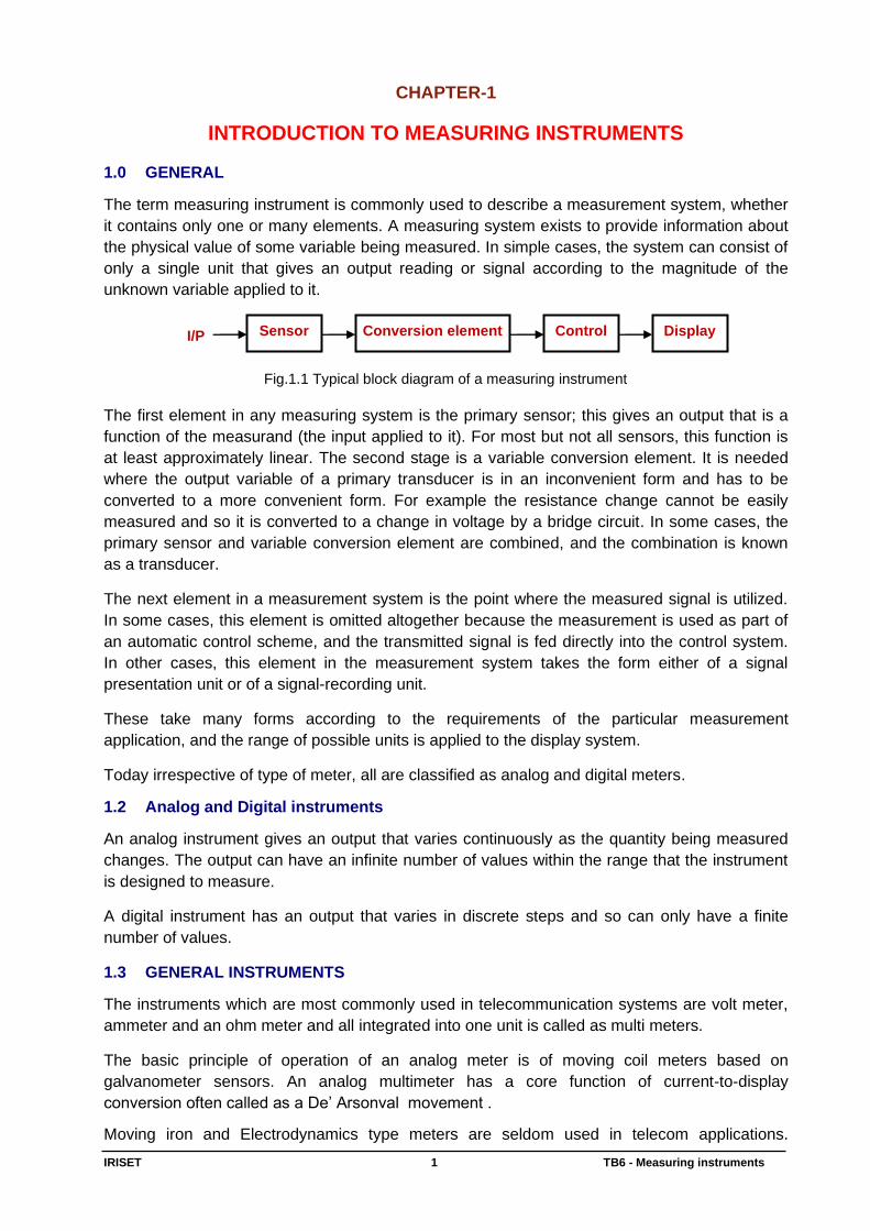
Fig.1.1 Typical block diagram of a measuring instrument
The first element in any measuring system is the primary sensor; this gives an output that is a
function of the measurand (the input applied to it). For most but not all sensors, this function is
at least approximately linear. The second stage is a variable conversion element. It is needed
where the output variable of a primary transducer is in an inconvenient form and has to be
converted to a more convenient form. For example the resistance change cannot be easily
measured and so it is converted to a change in voltage by a bridge circuit. In some cases, the
primary sensor and variable conversion element are combined, and the combination is known
as a transducer.
The next element in a measurement system is the point where the measured signal is utilized.
In some cases, this element is omitted altogether because the measurement is used as part of
an automatic control scheme, and the transmitted signal is fed directly into the control system.
In other cases, this element in the measurement system takes the form either of a signal
presentation unit or of a signal-recording unit.
These take many forms according to the requirements of the particular measurement
application, and the range of possible units is applied to the display system.
Today irrespective of type of meter, all are classified as analog and digital meters.
1.2 Analog and Digital instruments
An analog instrument gives an output that varies continuously as the quantity being measured
changes. The output can have an infinite number of values within the range that the instrument
is designed to measure.
A digital instrument has an output that varies in discrete steps and so can only have a finite
number of values.
1.3 GENERAL INSTRUMENTS
The instruments which are most commonly used in telecommunication systems are volt meter,
ammeter and an ohm meter and all integrated into one unit is called as multi meters.
The basic principle of operation of an analog meter is of moving coil meters based on
galvanometer sensors. An analog multimeter has a core function of current-to-display
conversion often called as a De’ Arsonval movement .
Moving iron and Electrodynamics type meters are seldom used in telecom applications.
Sensor Conversion element Control Display I/P
Introduction to Measuring Instruments
IRISET 2 TB6 - Measuring instruments
1.3.1 Permanent Magnet Moving Coil: Principle of Working
Construction
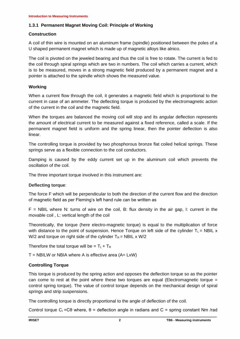
A coil of thin wire is mounted on an aluminum frame (spindle) positioned between the poles of a
U shaped permanent magnet which is made up of magnetic alloys like alnico.
The coil is pivoted on the jeweled bearing and thus the coil is free to rotate. The current is fed to
the coil through spiral springs which are two in numbers. The coil which carries a current, which
is to be measured, moves in a strong magnetic field produced by a permanent magnet and a
pointer is attached to the spindle which shows the measured value.
Working
When a current flow through the coil, it generates a magnetic field which is proportional to the
current in case of an ammeter. The deflecting torque is produced by the electromagnetic action
of the current in the coil and the magnetic field.
When the torques are balanced the moving coil will stop and its angular deflection represents
the amount of electrical current to be measured against a fixed reference, called a scale. If the
permanent magnet field is uniform and the spring linear, then the pointer deflection is also
linear.
The controlling torque is provided by two phosphorous bronze flat coiled helical springs. These
springs serve as a flexible connection to the coil conductors.
Damping is caused by the eddy current set up in the aluminum coil which prevents the
oscillation of the coil.
The three important torque involved in this instrument are: Deflecting torque:
The force F which will be perpendicular to both the direction of the current flow and the direction
of magnetic field as per Fleming’s left hand rule can be written as
F = NBIL where N: turns of wire on the coil, B: flux density in the air gap, I: current in the
movable coil , L: vertical length of the coil
Theoretically, the torque (here electro-magnetic torque) is equal to the multiplication of force
with distance to the point of suspension. Hence Torque on left side of the cylinder TL = NBIL x
W/2 and torque on right side of the cylinder TR = NBIL x W/2
Therefore the total torque will be = TL + TR
T = NBILW or NBIA where A is effective area (A= LxW) Controlling Torque
This torque is produced by the spring action and opposes the deflection torque so as the pointer
can come to rest at the point where these two torques are equal (Electromagnetic torque =
control spring torque). The value of control torque depends on the mechanical design of spiral
springs and strip suspensions.
The controlling torque is directly proportional to the angle of deflection of the coil.
Control torque Ct =Cθ where, θ = deflection angle in radians and C = spring constant Nm /rad
Introduction to Measuring Instruments
IRISET 3 TB6 - Measuring instruments
Fig 1,2 PMMC Construction
Damping torque This torque ensures the pointer comes to an equilibrium position i.e. at rest in the scale without
oscillating to give an accurate reading. In PMMC as the coil moves in the magnetic field, eddy
current sets up in a metal former or core on which the coil is wound or in the circuit of the coil
itself which opposes the motion of the coil resulting in the slow swing of a pointer and then
come to rest quickly with very little oscillation.
Applications The PMMC can be used as: 1) Ammeter: When PMMC is used as an ammeter, except for a very small current range, the moving coil is
connected across a suitable low resistance shunt, so that only small part of the main current
flows through the coil.
The shunt consists of a number of thin plates made up of alloy metal, which is usually magnetic
and has a low-temperature coefficient of resistance, fixed between two massive blocks of
copper. A resistor of the same alloy is also placed in series with the coil to reduce errors due to
temperature variation.
2) Voltmeter: When PMMC is used as a voltmeter, the coil is connected in series with a high resistance. Rest
of the function is same as above. The same moving coil can be used as an ammeter or
voltmeter with an interchange of above arrangement
Introduction to Measuring Instruments
IRISET 4 TB6 - Measuring instruments
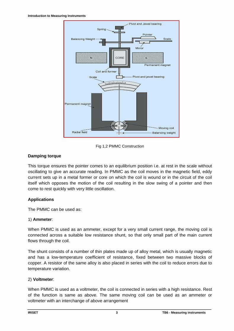
Fig 1.3
3) Ohm Meter: The ohm meter is used to measure the resistance of the electric circuit by applying a voltage to
a resistance with the help of battery. A galvanometer is used to determine the flow of current
through the resistance. The galvanometer scale is marked in ohms and as the resistance varies
since the voltage is fixed, the current through the meter will also vary.
4) Galvanometer: The galvanometer is used to measure a small value of current along with its direction and
strength. It is mainly used onboard to detect and compare different circuits in a system.
Advantages • The PMMC consumes less power and has great accuracy.
• It has a uniformly divided scale and can cover an arc of 270 degrees.
• The PMMC has a high torque to weight ratio.
• It can be modified as ammeter or voltmeter with suitable resistance.
• It has efficient damping characteristics and is not affected by stray magnetic field.
• It produces no losses due to hysteresis.
Disadvantage • The moving coil instrument can only be used on D.C supply as the reversal of current
produces a reversal of torque on the coil.
• It’s very delicate and sometimes uses AC circuit with a rectifier.
• It’s costly as compared to moving coil iron instruments.
• It may show an error due to loss of magnetism of permanent magnet.
Introduction to Measuring Instruments
IRISET 5 TB6 - Measuring instruments
What are the different reasons that cause an error in PMMC?
Temperature effect: Error in the reading of the PMMC may cause due to change in the
temperature which will affect the resistance of the moving coil. The temperature coefficients
of the value of the coefficient of copper wire in moving coil are 0.04 per degree Celsius rise
in temperature. Since the coil has a lower temperature coefficient, it will have a faster rate
of temperature rises which will result in increase in the resistance causing an error
Spring material and age: The other factor which may lead to error in the PMMC reading is
the quality and contortion of the spring. Old aging spring will not allow the pointer to show
the correct reading making an error.
Ageing of Magnet: Along with the age, the effect of heat and vibration will reduce the
magnetic effect of the permanent magnet which will produce an error in the reading.
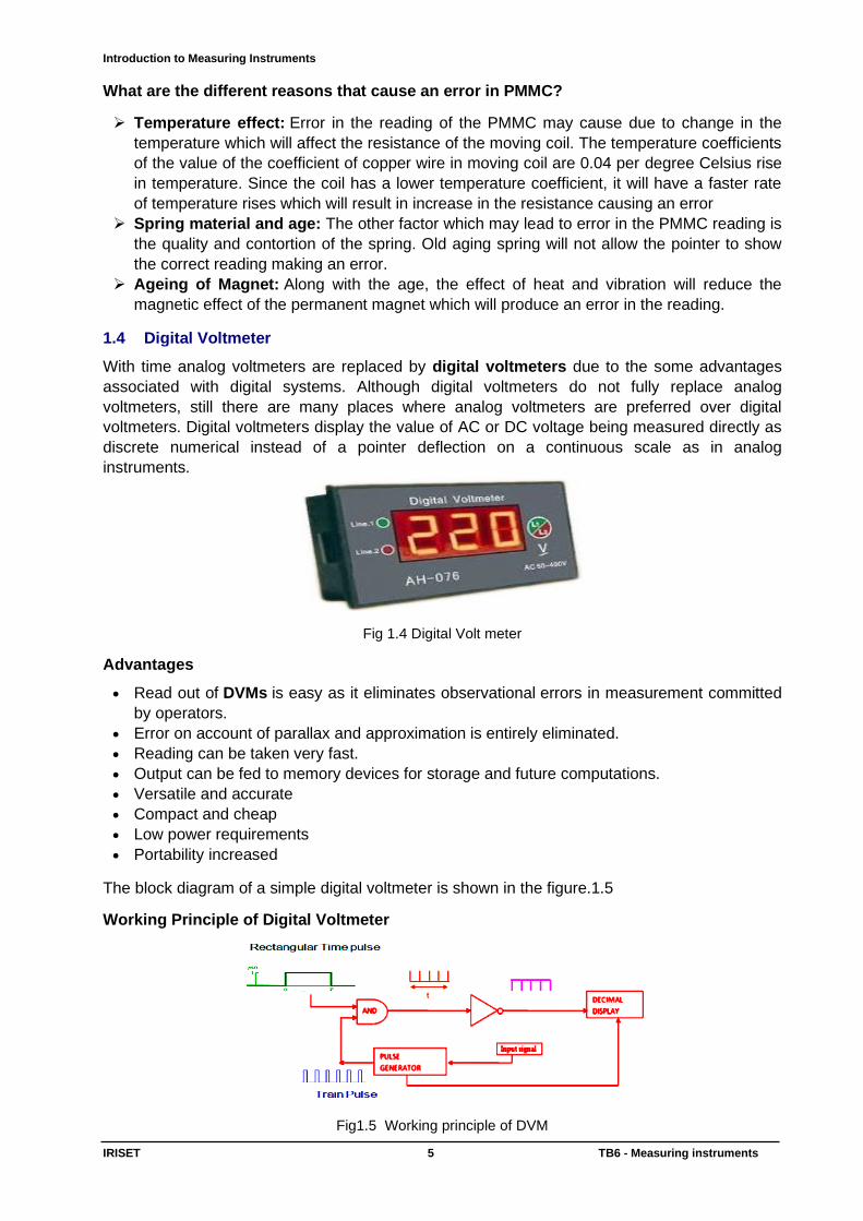
1.4 Digital Voltmeter
With time analog voltmeters are replaced by digital voltmeters due to the some advantages
associated with digital systems. Although digital voltmeters do not fully replace analog
voltmeters, still there are many places where analog voltmeters are preferred over digital
voltmeters. Digital voltmeters display the value of AC or DC voltage being measured directly as
discrete numerical instead of a pointer deflection on a continuous scale as in analog
instruments.
Fig 1.4 Digital Volt meter
Advantages
• Read out of DVMs is easy as it eliminates observational errors in measurement committed
by operators.
• Error on account of parallax and approximation is entirely eliminated.
• Reading can be taken very fast.
• Output can be fed to memory devices for storage and future computations.
• Versatile and accurate
• Compact and cheap
• Low power requirements
• Portability increased
The block diagram of a simple digital voltmeter is shown in the figure.1.5
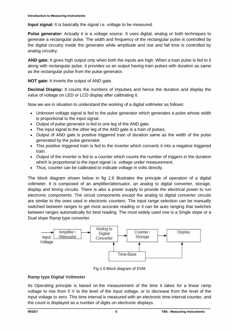
Working Principle of Digital Voltmeter
Fig1.5 Working principle of DVM
Introduction to Measuring Instruments
IRISET 6 TB6 - Measuring instruments
Input signal: It is basically the signal i.e. voltage to be measured.
Pulse generator: Actually it is a voltage source. It uses digital, analog or both techniques to
generate a rectangular pulse. The width and frequency of the rectangular pulse is controlled by
the digital circuitry inside the generator while amplitude and rise and fall time is controlled by
analog circuitry.
AND gate: It gives high output only when both the inputs are high. When a train pulse is fed to it
along with rectangular pulse, it provides us an output having train pulses with duration as same
as the rectangular pulse from the pulse generator.
NOT gate: It inverts the output of AND gate.
Decimal Display: It counts the numbers of impulses and hence the duration and display the
value of voltage on LED or LCD display after calibrating it.
Now we are in situation to understand the working of a digital voltmeter as follows:
• Unknown voltage signal is fed to the pulse generator which generates a pulse whose width
is proportional to the input signal.
• Output of pulse generator is fed to one leg of the AND gate.
• The input signal to the other leg of the AND gate is a train of pulses.
• Output of AND gate is positive triggered train of duration same as the width of the pulse
generated by the pulse generator.
• This positive triggered train is fed to the inverter which converts it into a negative triggered
train.
• Output of the inverter is fed to a counter which counts the number of triggers in the duration
which is proportional to the input signal i.e. voltage under measurement.
• Thus, counter can be calibrated to indicate voltage in volts directly.
The block diagram shown below in fig 1.6 illustrates the principle of operation of a digital
voltmeter. It is composed of an amplifier/attenuator, an analog to digital converter, storage,
display and timing circuits. There is also a power supply to provide the electrical power to run
electronic components. The circuit components except the analog to digital converter circuits
are similar to the ones used in electronic counters. The input range selection can be manually
switched between ranges to get most accurate reading or it can be auto ranging that switches
between ranges automatically for best reading. The most widely used one is a Single slope or a
Dual slope Ramp type converter.
Fig 1.6 Block diagram of DVM
Ramp type Digital Voltmeter
Its Operating principle is based on the measurement of the time it takes for a linear ramp
voltage to rise from 0 V to the level of the input voltage, or to decrease from the level of the
input voltage to zero. This time interval is measured with an electronic time-interval counter, and
the count is displayed as a number of digits on electronic displays.
Introduction to Measuring Instruments
IRISET 7 TB6 - Measuring instruments
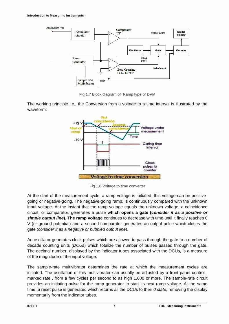
Fig 1.7 Block diagram of Ramp type of DVM
The working principle i.e., the Conversion from a voltage to a time interval is illustrated by the
waveform:
Fig 1.8 Voltage to time converter
At the start of the measurement cycle, a ramp voltage is initiated; this voltage can be positive-
going or negative-going. The negative-going ramp, is continuously compared with the unknown
input voltage. At the instant that the ramp voltage equals the unknown voltage, a coincidence
circuit, or comparator, generates a pulse which opens a gate (consider it as a positive or
simple output line). The ramp voltage continues to decrease with time until it finally reaches 0
V (or ground potential) and a second comparator generates an output pulse which closes the
gate (consider it as a negative or bubbled output line).
An oscillator generates clock pulses which are allowed to pass through the gate to a number of
decade counting units (DCUs) which totalize the number of pulses passed through the gate.
The decimal number, displayed by the indicator tubes associated with the DCUs, is a measure
of the magnitude of the input voltage.
The sample-rate multivibrator determines the rate at which the measurement cycles are
initiated. The oscillation of this multivibrator can usually be adjusted by a front-panel control ,
marked rate , from a few cycles per second to as high 1,000 or more. The sample-rate circuit
provides an initiating pulse for the ramp generator to start its next ramp voltage. At the same
time, a reset pulse is generated which returns all the DCUs to their 0 state, removing the display
momentarily from the indicator tubes.
Introduction to Measuring Instruments
IRISET 8 TB6 - Measuring instruments
Dual slope integrating type Digital Voltmeter The ramp type DVM (single slope) is very simple yet has several drawbacks. The major
limitation is the sensitivity of the output to system components and clock. The dual slope
techniques eliminate the sensitivities and hence the mostly implemented approach in DVMs.
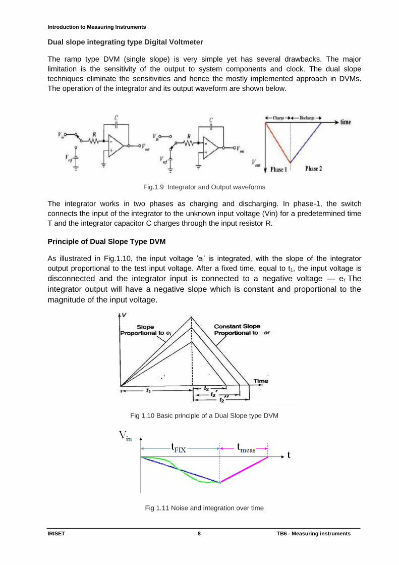
The operation of the integrator and its output waveform are shown below.
Fig.1.9 Integrator and Output waveforms
The integrator works in two phases as charging and discharging. In phase-1, the switch
connects the input of the integrator to the unknown input voltage (Vin) for a predetermined time
T and the integrator capacitor C charges through the input resistor R.
Principle of Dual Slope Type DVM As illustrated in Fig.1.10, the input voltage ’ei’ is integrated, with the slope of the integrator
output proportional to the test input voltage. After a fixed time, equal to t1, the input voltage is
disconnected and the integrator input is connected to a negative voltage — er The
integrator output will have a negative slope which is constant and proportional to the
magnitude of the input voltage.
Fig 1.10 Basic principle of a Dual Slope type DVM
Fig 1.11 Noise and integration over time
Introduction to Measuring Instruments
IRISET 9 TB6 - Measuring instruments
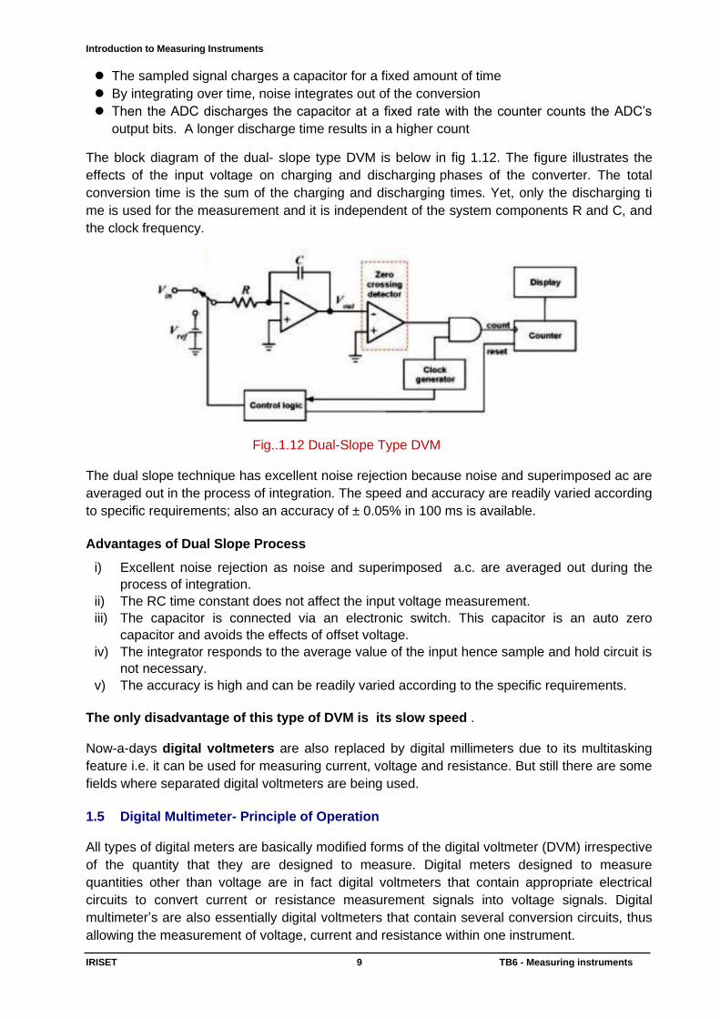
The sampled signal charges a capacitor for a fixed amount of time
By integrating over time, noise integrates out of the conversion
Then the ADC discharges the capacitor at a fixed rate with the counter counts the ADC’s
output bits. A longer discharge time results in a higher count
The block diagram of the dual- slope type DVM is below in fig 1.12. The figure illustrates the
effects of the input voltage on charging and discharging phases of the converter. The total
conversion time is the sum of the charging and discharging times. Yet, only the discharging ti
me is used for the measurement and it is independent of the system components R and C, and
the clock frequency.
Fig..1.12 Dual-Slope Type DVM The dual slope technique has excellent noise rejection because noise and superimposed ac are
averaged out in the process of integration. The speed and accuracy are readily varied according
to specific requirements; also an accuracy of ± 0.05% in 100 ms is available.
Advantages of Dual Slope Process
i) Excellent noise rejection as noise and superimposed a.c. are averaged out during the
process of integration.
ii) The RC time constant does not affect the input voltage measurement.
iii) The capacitor is connected via an electronic switch. This capacitor is an auto zero
capacitor and avoids the effects of offset voltage.
iv) The integrator responds to the average value of the input hence sample and hold circuit is
not necessary.
v) The accuracy is high and can be readily varied according to the specific requirements.
The only disadvantage of this type of DVM is its slow speed . Now-a-days digital voltmeters are also replaced by digital millimeters due to its multitasking
feature i.e. it can be used for measuring current, voltage and resistance. But still there are some
fields where separated digital voltmeters are being used.
1.5 Digital Multimeter- Principle of Operation All types of digital meters are basically modified forms of the digital voltmeter (DVM) irrespective
of the quantity that they are designed to measure. Digital meters designed to measure
quantities other than voltage are in fact digital voltmeters that contain appropriate electrical
circuits to convert current or resistance measurement signals into voltage signals. Digital
multimeter’s are also essentially digital voltmeters that contain several conversion circuits, thus
allowing the measurement of voltage, current and resistance within one instrument.
Introduction to Measuring Instruments
IRISET 10 TB6 - Measuring instruments
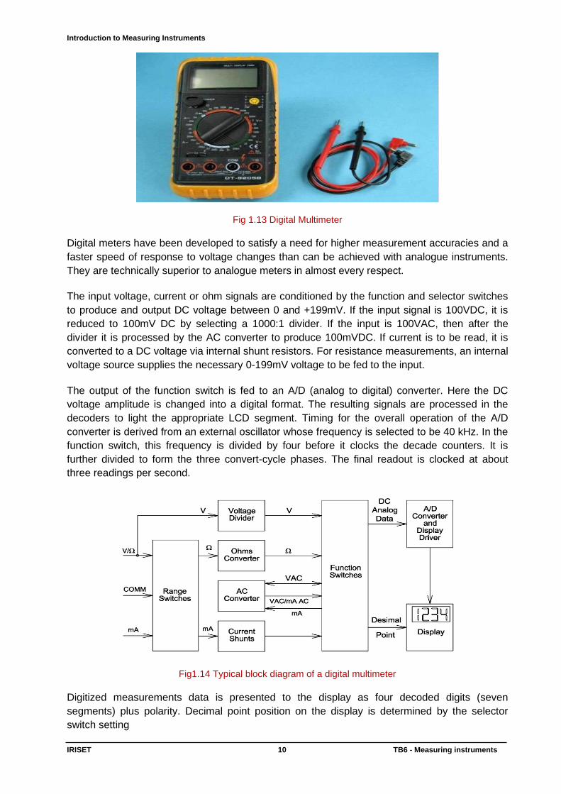
Fig 1.13 Digital Multimeter
Digital meters have been developed to satisfy a need for higher measurement accuracies and a
faster speed of response to voltage changes than can be achieved with analogue instruments.
They are technically superior to analogue meters in almost every respect.
The input voltage, current or ohm signals are conditioned by the function and selector switches
to produce and output DC voltage between 0 and +199mV. If the input signal is 100VDC, it is
reduced to 100mV DC by selecting a 1000:1 divider. If the input is 100VAC, then after the
divider it is processed by the AC converter to produce 100mVDC. If current is to be read, it is
converted to a DC voltage via internal shunt resistors. For resistance measurements, an internal
voltage source supplies the necessary 0-199mV voltage to be fed to the input.
The output of the function switch is fed to an A/D (analog to digital) converter. Here the DC
voltage amplitude is changed into a digital format. The resulting signals are processed in the
decoders to light the appropriate LCD segment. Timing for the overall operation of the A/D
converter is derived from an external oscillator whose frequency is selected to be 40 kHz. In the
function switch, this frequency is divided by four before it clocks the decade counters. It is
further divided to form the three convert-cycle phases. The final readout is clocked at about
three readings per second.
Fig1.14 Typical block diagram of a digital multimeter
Digitized measurements data is presented to the display as four decoded digits (seven
segments) plus polarity. Decimal point position on the display is determined by the selector
switch setting
Introduction to Measuring Instruments
IRISET 11 TB6 - Measuring instruments
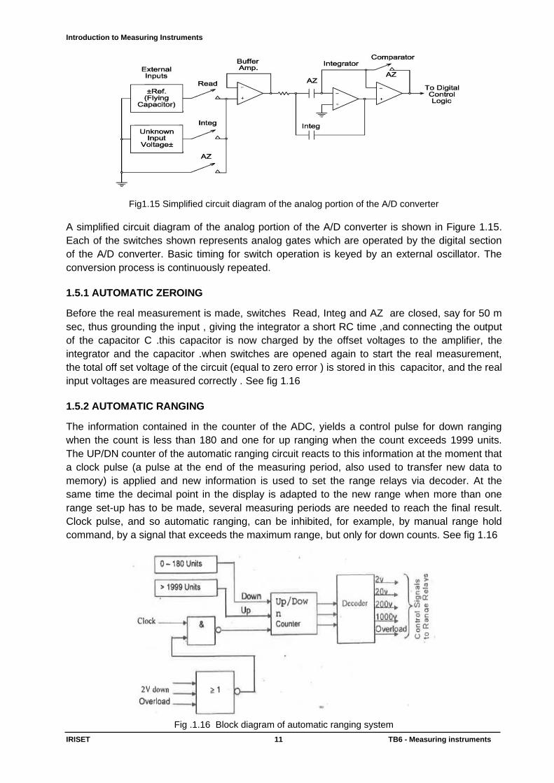
Fig1.15 Simplified circuit diagram of the analog portion of the A/D converter
A simplified circuit diagram of the analog portion of the A/D converter is shown in Figure 1.15.
Each of the switches shown represents analog gates which are operated by the digital section
of the A/D converter. Basic timing for switch operation is keyed by an external oscillator. The
conversion process is continuously repeated.
1.5.1 AUTOMATIC ZEROING
Before the real measurement is made, switches Read, Integ and AZ are closed, say for 50 m
sec, thus grounding the input , giving the integrator a short RC time ,and connecting the output
of the capacitor C .this capacitor is now charged by the offset voltages to the amplifier, the
integrator and the capacitor .when switches are opened again to start the real measurement,
the total off set voltage of the circuit (equal to zero error ) is stored in this capacitor, and the real
input voltages are measured correctly . See fig 1.16
1.5.2 AUTOMATIC RANGING
The information contained in the counter of the ADC, yields a control pulse for down ranging
when the count is less than 180 and one for up ranging when the count exceeds 1999 units.
The UP/DN counter of the automatic ranging circuit reacts to this information at the moment that
a clock pulse (a pulse at the end of the measuring period, also used to transfer new data to
memory) is applied and new information is used to set the range relays via decoder. At the
same time the decimal point in the display is adapted to the new range when more than one
range set-up has to be made, several measuring periods are needed to reach the final result.
Clock pulse, and so automatic ranging, can be inhibited, for example, by manual range hold
command, by a signal that exceeds the maximum range, but only for down counts. See fig 1.16
Fig .1.16 Block diagram of automatic ranging system

Introduction to Measuring Instruments
IRISET 12 TB6 - Measuring instruments
Any given measurement cycle performed by the A/D converter can be divided into three
consecutive time periods: Auto zero (AZ), integrate (INTEG) and READ. Both auto zero and
integrate are fixed time periods. A counter determines the length of both time periods by
providing an overflow at the end of every 1,000 clock pulses. The read period is a variable time,
which is proportional to the unknown input voltage. The value of the voltage is determined by
counting the number of clock pulses that occur during the read period.
Fig 1.17 Measurement period
Note that there are 3- and 4-digit (and more) DMMs, plus 3-1/2, 3-3/4, 4-1/2, etc. A 3-1/2 digit
meter reads 000-999 plus 1000 to 1999. Since this is twice as high as a 3-digit meter can read,
it is arbitrarily called a 3-1/2 digit. A seven-segment display for this only needs the two segments
that make up a "1" to perform this function. A 3-3/4 digit meter reads 000-3999, doubling the
range again, but saving only one segment compared to a full 4-digit display. One could define a
3-7/8 digit meter as extending to 7999, and use a regular 4-digit display, but this is not normally
done, since you are practically at the next level but probably have to charge less for it.
1.5.3 VOLTAGE MEASUREMENT
Fig1.18 Simplified Voltage Measurement Diagram
The input divider resistors add up 10MΩ with each step being a division of 10. The divider
output should be within –0.199 to +0.199V or the overload indicator will function. If the AC
function is selected, the divider output is AC coupled to a full wave rectifier and the DC output is
calibrated to equal the rms level of the AC input.
1.5.4 CURRENT MEASUREMENT
Figure 1.19 shows a simplified diagram of the current measurement positions. Internal shunt
resistors convert the current to between –0.199 to and 0.199V which is then processed in the IC
to light the appropriate LCD segments. If the current is AC in nature, the AC converter changes
it to the equivalent DC value.
Introduction to Measuring Instruments
IRISET 13 TB6 - Measuring instruments
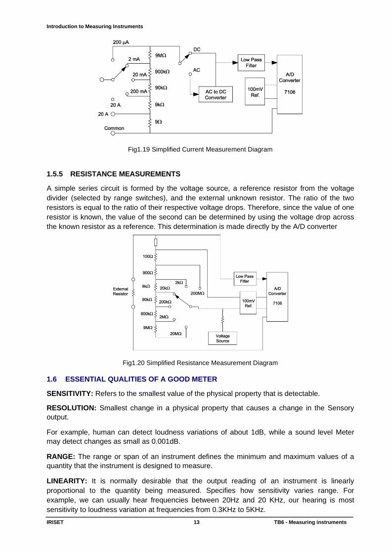
Fig1.19 Simplified Current Measurement Diagram
1.5.5 RESISTANCE MEASUREMENTS
A simple series circuit is formed by the voltage source, a reference resistor from the voltage
divider (selected by range switches), and the external unknown resistor. The ratio of the two
resistors is equal to the ratio of their respective voltage drops. Therefore, since the value of one
resistor is known, the value of the second can be determined by using the voltage drop across
the known resistor as a reference. This determination is made directly by the A/D converter
Fig1.20 Simplified Resistance Measurement Diagram
1.6 ESSENTIAL QUALITIES OF A GOOD METER
SENSITIVITY: Refers to the smallest value of the physical property that is detectable.
RESOLUTION: Smallest change in a physical property that causes a change in the Sensory
output.
For example, human can detect loudness variations of about 1dB, while a sound level Meter
may detect changes as small as 0.001dB.
RANGE: The range or span of an instrument defines the minimum and maximum values of a
quantity that the instrument is designed to measure.
LINEARITY: It is normally desirable that the output reading of an instrument is linearly
proportional to the quantity being measured. Specifies how sensitivity varies range. For
example, we can usually hear frequencies between 20Hz and 20 KHz, our hearing is most
sensitivity to loudness variation at frequencies from 0.3KHz to 5KHz.
Introduction to Measuring Instruments
IRISET 14 TB6 - Measuring instruments
PRECISION: Refers to the reproducibility or repeatability of an observation. The terms repeatability and reproducibility mean approximately the same but are applied in
different contexts as given below.
Repeatability describes the closeness of output readings when the same input is applied
repetitively over a short period of time, with the same measurement conditions, same instrument
and observer, same location and same conditions of use maintained throughout.
Reproducibility describes the closeness of output readings for the same input when there are
changes in the method of measurement, observer, measuring instrument, location, conditions of
use and time of measurement.
Both terms thus describe the spread of output readings for the same input. This spread is
referred to as repeatability if the measurement conditions are constant and as reproducibility if
the measurement conditions vary.
LAG AND SETTING TIME: Refers to the amount of time that lapses between the initiation of an
observation and the final output of information.
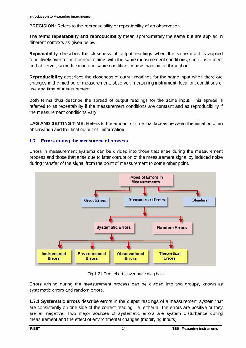
1.7 Errors during the measurement process Errors in measurement systems can be divided into those that arise during the measurement
process and those that arise due to later corruption of the measurement signal by induced noise
during transfer of the signal from the point of measurement to some other point.
Fig 1.21 Error chart cover page diag back
Errors arising during the measurement process can be divided into two groups, known as
systematic errors and random errors.
1.7.1 Systematic errors describe errors in the output readings of a measurement system that
are consistently on one side of the correct reading, i.e. either all the errors are positive or they
are all negative. Two major sources of systematic errors are system disturbance during
measurement and the effect of environmental changes (modifying inputs)
Introduction to Measuring Instruments
IRISET 15 TB6 - Measuring instruments
Sources of systematic error Systematic errors in the output of many instruments are due
to factors inherent in the manufacture of the instrument arising out of tolerances in the
components of the instrument. They can also arise due to wear in instrument components
over a period of time. In other cases, systematic errors are introduced either by the effect of
environmental disturbances or through the disturbance of the measured system by the act
of measurement. Disturbance of the measured system by the act of measurement is a
common source of systematic error.
System disturbance due to measurement Disturbance of the measured system by the act of measurement is a common source of
systematic error.
1.7.2 Random errors are perturbations (disturbance) of the measurement either side of the
true value caused by random and unpredictable effects, such that positive errors and negative
errors occur in approximately equal numbers for a series of measurements made of the same
quantity. Such perturbations are mainly small, but large perturbations occur from time to time
unpredictably. Random errors often arise when measurements are taken by human observation
of an analogue meter, especially where this involves interpolation between scale points.
Electrical noise can also be a source of random errors. To a large extent, random errors can be
overcome by taking the same measurement a number of times and extracting a value by
averaging or other statistical techniques. However, any quantification of the measurement value
and statement of error bounds remains a statistical quantity.
Finally, a word must be said about the distinction between systematic and random errors. Error
sources in the measurement system must be examined carefully to determine what type of error
is present, systematic or random, and to apply the appropriate treatment.
1.8 Calibration of measuring instruments 1.8.1 Principles of calibration Calibration consists of comparing the output of the instrument or sensor under test against the
output of an instrument of known accuracy when the same input (the measured quantity) is
applied to both instruments. This procedure is carried out for a range of inputs covering the
whole measurement range of the instrument or sensor.
Calibration ensures that the measuring accuracy of all instruments and sensors used in a
measurement system is known over the whole measurement range, provided that the calibrated
instruments and sensors are used in environmental conditions that are the same as those under
which they were calibrated
All instruments suffer drift in their characteristics, and the rate at which this happens depends on
many factors, such as the environmental conditions in which instruments are used and the
frequency of their use. Thus, errors due to instruments being out of calibration can usually be
rectified by increasing the frequency of recalibration.
1.8.2 Calibration chain and traceability The calibration facilities provided within the instrumentation department of a company provide
the first link in the calibration chain. Instruments used for calibration at this level are known as
working standards. As such working standard instruments are kept by the instrumentation
Introduction to Measuring Instruments
IRISET 16 TB6 - Measuring instruments
department of a company solely for calibration duties, and for no other purpose, then it can be
assumed that they will maintain their accuracy over a reasonable period of time because use-
related deterioration in accuracy is largely eliminated
The instrument used for calibrating working standard instruments is known as a secondary
reference standard. This must obviously be a very well-engineered instrument that gives high
accuracy and is stabilized against drift in its performance with time. When the working standard
instrument has been calibrated by an authorized standards laboratory, a calibration certificate
will be issued. This will contain at least the following information.
• the identification of the equipment calibrated
• the calibration results obtained
• the measurement uncertainty
• any use limitations on the equipment calibrated
• the date of calibration
• the authority under which the certificate is issued.
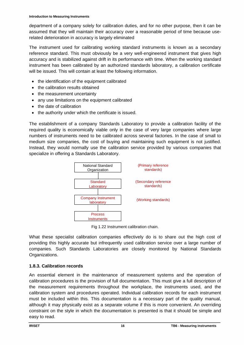
The establishment of a company Standards Laboratory to provide a calibration facility of the
required quality is economically viable only in the case of very large companies where large
numbers of instruments need to be calibrated across several factories. In the case of small to
medium size companies, the cost of buying and maintaining such equipment is not justified.
Instead, they would normally use the calibration service provided by various companies that
specialize in offering a Standards Laboratory.
Fig 1.22 Instrument calibration chain.
What these specialist calibration companies effectively do is to share out the high cost of
providing this highly accurate but infrequently used calibration service over a large number of
companies. Such Standards Laboratories are closely monitored by National Standards
Organizations.
1.8.3. Calibration records
An essential element in the maintenance of measurement systems and the operation of
calibration procedures is the provision of full documentation. This must give a full description of
the measurement requirements throughout the workplace, the instruments used, and the
calibration system and procedures operated. Individual calibration records for each instrument
must be included within this. This documentation is a necessary part of the quality manual,
although it may physically exist as a separate volume if this is more convenient. An overriding
constraint on the style in which the documentation is presented is that it should be simple and
easy to read.
National Standard Organization
Standard
Laboratory
Company Instrument laboratory
Process
Instruments
(Primary reference standards)
(Secondary reference standards)
(Working standards)
Introduction to Measuring Instruments
IRISET 17 TB6 - Measuring instruments
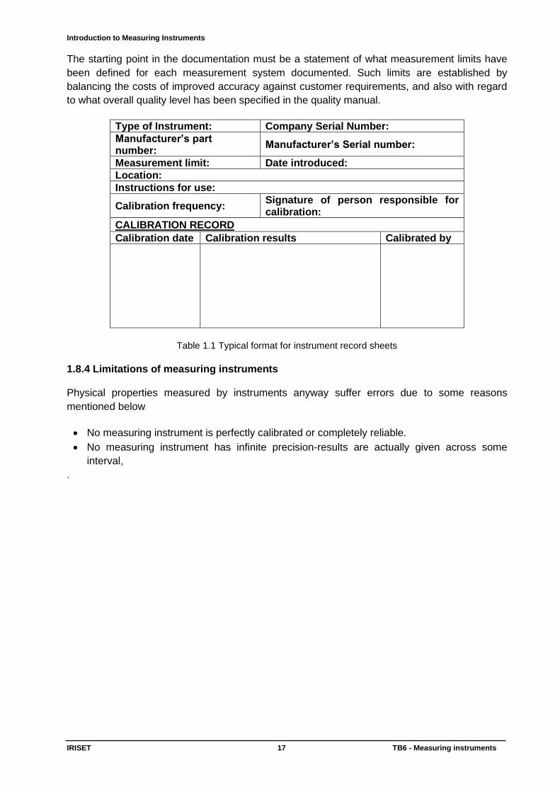
The starting point in the documentation must be a statement of what measurement limits have
been defined for each measurement system documented. Such limits are established by
balancing the costs of improved accuracy against customer requirements, and also with regard
to what overall quality level has been specified in the quality manual.
Type of Instrument: Company Serial Number:
Manufacturer’s part number:
Manufacturer’s Serial number:
Measurement limit: Date introduced:
Location:
Instructions for use:
Calibration frequency: Signature of person responsible for calibration:
CALIBRATION RECORD
Calibration date Calibration results Calibrated by
Table 1.1 Typical format for instrument record sheets
1.8.4 Limitations of measuring instruments Physical properties measured by instruments anyway suffer errors due to some reasons
mentioned below
• No measuring instrument is perfectly calibrated or completely reliable.
• No measuring instrument has infinite precision-results are actually given across some
interval,
.
Outdoor (Field) Measuring Instruments
IRISET 18 TB6 - Measuring instruments
CHAPTER-2
OUTDOOR (FIELD) MEASURING INSTRUMENTS 2.0 GENERAL
The outdoor (field) measuring instruments used in telecommunication systems are generally on
underground copper cables of various types, overhead (ACSR) lines and systems. The general
types of faults found on transmission lines are following:-
1. Earth fault: When the insulation between the earth and the conductor in the cable becomes
very low.
2. Low insulation fault.: When the insulation between conductors in the cable or between the
pairs or between pair and earth falls below a prescribed limit (normally 0.5 meg ohm) This
may be due to entry of moisture or due to failure of wire insulation.
3. Disconnection Fault: When the Conductor is cut then the fault is called break fault or is
called High Resistance fault when High Resistance is introduced in the circuit.
4. Short Circuit Fault: When the resistance between the wires or between the conductors
becomes very low even without any loop in the circuit on the pairs. This is also called
contact fault.
5. Foreign potential :The existence of potential, even when the circuit is idle or isolated from
the potential of exchange
6. Noise: Highly objectionable on voice circuits arising from several intrinsic and extrinsic
reasons.
Various types of measurements taken periodically on transmission lines , during installation and
maintenance are classified as-
Insulation resistance
Route tracing
Fault locating
Earth resistance
Transmission losses
Measurement of Noise
For the above said measurements, the measuring instruments used are megger, cable route
tracer, cable fault locator, earth tester and transmission measuring set respectively.
2.1. INSULATION RESISTANCE MEASUREMENT
The purpose to check insulation resistance of underground cables: The insulation is used
to separate the conductors bunched in a unit to prevent short circuit between two conductors in
a pair or between conductors of one pair with the conductor any other pair in the unit or core in
the cable. The insulation is used as SHEATH to separate the insulated conductors from being
corroded or eroded in soil. The insulation is being used for marking / identifying the pair or
conductor in the unit and in the cable as a whole for that matter. The insulating material is used
for preventing the grounding or earthing of the conductors and also used for preventing the
corrosion of armoring.
2.1.1 INSULATION TESTER ( MEGGER )
Megger working principle is based on the working principle of moving coil instruments, which
states that when a current carrying conductor is placed in a magnetic field, a mechanical force is
experienced by it.
Outdoor (Field) Measuring Instruments
IRISET 19 TB6 - Measuring instruments
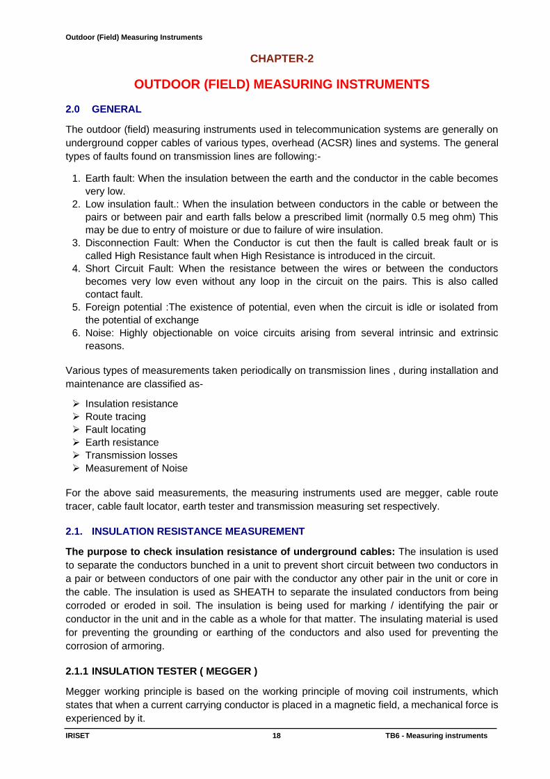
The magnitude and direction of this force depend upon the strength and direction of
the current and magnetic field. . Face panel of a Megger is shown in fig.2.1
Fig 2.1 Face panel of a Megger
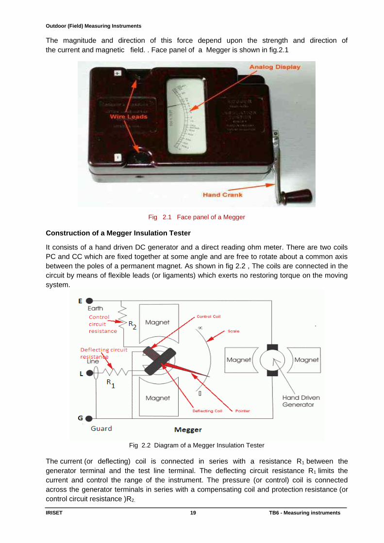
Construction of a Megger Insulation Tester
It consists of a hand driven DC generator and a direct reading ohm meter. There are two coils
PC and CC which are fixed together at some angle and are free to rotate about a common axis
between the poles of a permanent magnet. As shown in fig 2.2 , The coils are connected in the
circuit by means of flexible leads (or ligaments) which exerts no restoring torque on the moving
system.
Fig 2.2 Diagram of a Megger Insulation Tester
The current (or deflecting) coil is connected in series with a resistance R1 between the
generator terminal and the test line terminal. The deflecting circuit resistance R1 limits the
current and control the range of the instrument. The pressure (or control) coil is connected
across the generator terminals in series with a compensating coil and protection resistance (or
control circuit resistance )R2.
Outdoor (Field) Measuring Instruments
IRISET 20 TB6 - Measuring instruments
Compensating coil is connected to obtain better scale proportions. A guard ring is provided to
shunt leakage current over the test terminals or within the instrument itself. The terminal ‘G’
known as guard terminal is provided by means of which the guard ring can be connected to a
guard wire on the insulation under test. The test voltage generated by the generator is usually
500 or 1000 volts.
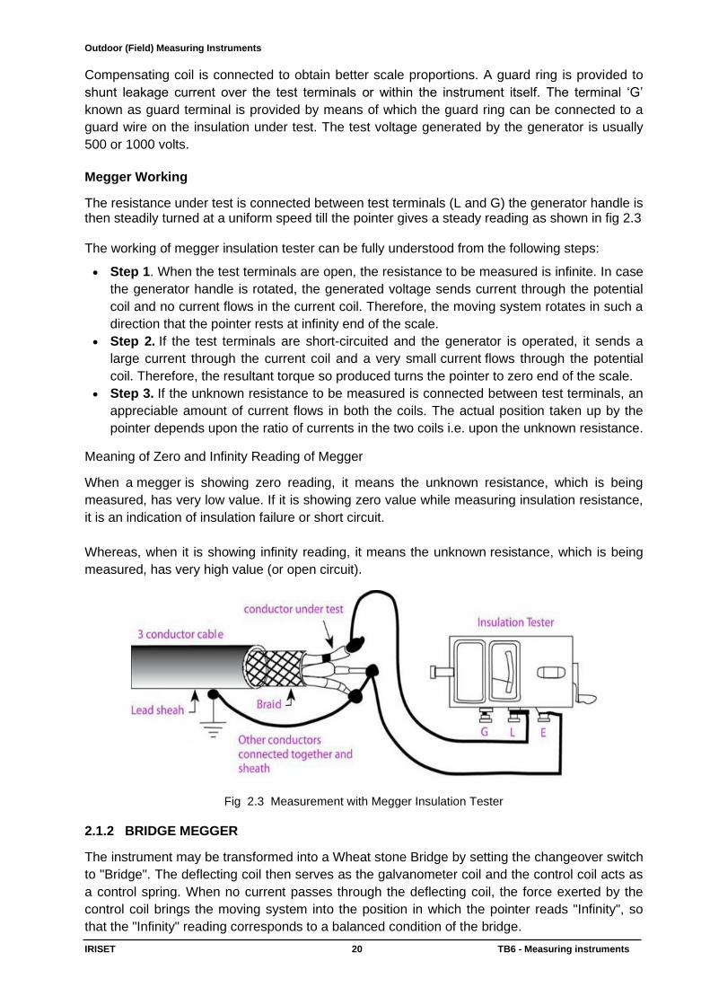
Megger Working
The resistance under test is connected between test terminals (L and G) the generator handle is then steadily turned at a uniform speed till the pointer gives a steady reading as shown in fig 2.3 The working of megger insulation tester can be fully understood from the following steps:
• Step 1. When the test terminals are open, the resistance to be measured is infinite. In case
the generator handle is rotated, the generated voltage sends current through the potential
coil and no current flows in the current coil. Therefore, the moving system rotates in such a
direction that the pointer rests at infinity end of the scale.
• Step 2. If the test terminals are short-circuited and the generator is operated, it sends a
large current through the current coil and a very small current flows through the potential
coil. Therefore, the resultant torque so produced turns the pointer to zero end of the scale.
• Step 3. If the unknown resistance to be measured is connected between test terminals, an
appreciable amount of current flows in both the coils. The actual position taken up by the
pointer depends upon the ratio of currents in the two coils i.e. upon the unknown resistance.
Meaning of Zero and Infinity Reading of Megger
When a megger is showing zero reading, it means the unknown resistance, which is being
measured, has very low value. If it is showing zero value while measuring insulation resistance,
it is an indication of insulation failure or short circuit.
Whereas, when it is showing infinity reading, it means the unknown resistance, which is being
measured, has very high value (or open circuit).
Fig 2.3 Measurement with Megger Insulation Tester
2.1.2 BRIDGE MEGGER
The instrument may be transformed into a Wheat stone Bridge by setting the changeover switch
to "Bridge". The deflecting coil then serves as the galvanometer coil and the control coil acts as
a control spring. When no current passes through the deflecting coil, the force exerted by the
control coil brings the moving system into the position in which the pointer reads "Infinity", so
that the "Infinity" reading corresponds to a balanced condition of the bridge.
Outdoor (Field) Measuring Instruments
IRISET 21 TB6 - Measuring instruments
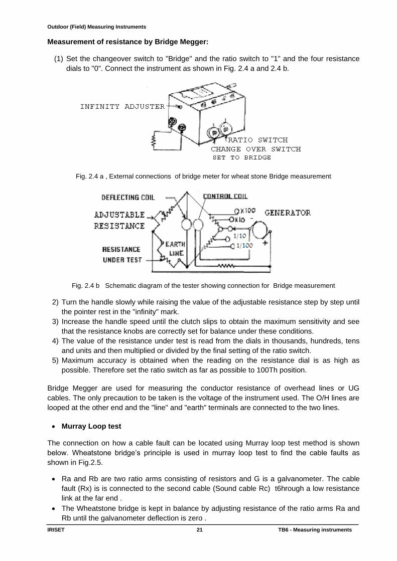
Measurement of resistance by Bridge Megger:
(1) Set the changeover switch to "Bridge" and the ratio switch to "1" and the four resistance
dials to "0". Connect the instrument as shown in Fig. 2.4 a and 2.4 b.
Fig. 2.4 a , External connections of bridge meter for wheat stone Bridge measurement
Fig. 2.4 b Schematic diagram of the tester showing connection for Bridge measurement
2) Turn the handle slowly while raising the value of the adjustable resistance step by step until
the pointer rest in the "infinity" mark.
3) Increase the handle speed until the clutch slips to obtain the maximum sensitivity and see
that the resistance knobs are correctly set for balance under these conditions.
4) The value of the resistance under test is read from the dials in thousands, hundreds, tens
and units and then multiplied or divided by the final setting of the ratio switch.
5) Maximum accuracy is obtained when the reading on the resistance dial is as high as
possible. Therefore set the ratio switch as far as possible to 100Th position.
Bridge Megger are used for measuring the conductor resistance of overhead lines or UG
cables. The only precaution to be taken is the voltage of the instrument used. The O/H lines are
looped at the other end and the "line" and "earth" terminals are connected to the two lines.
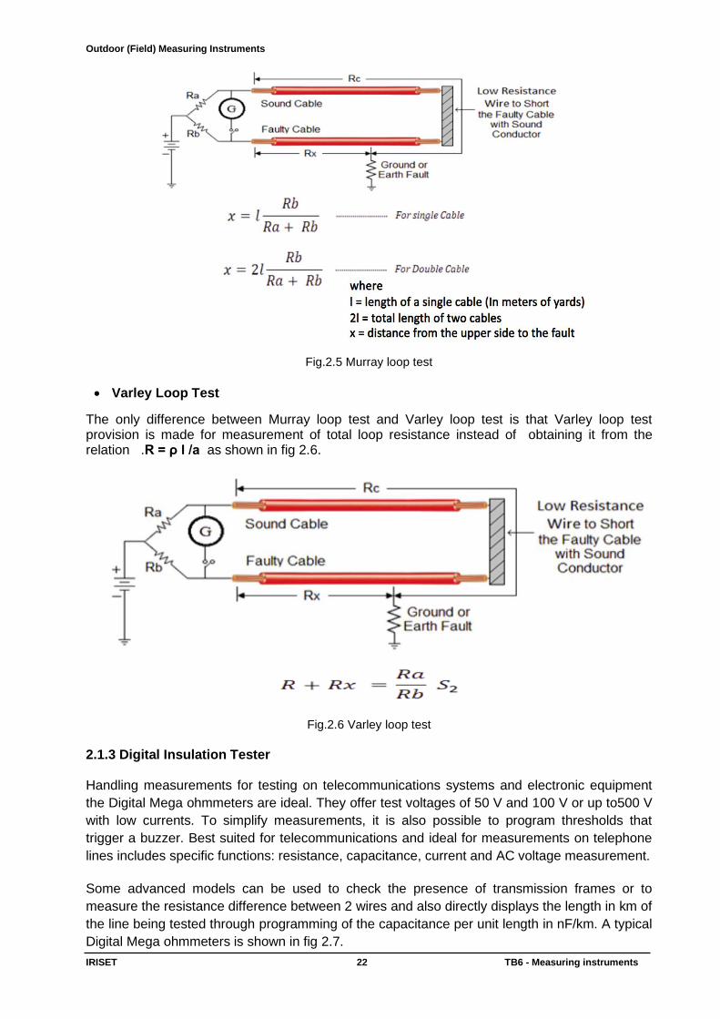
• Murray Loop test The connection on how a cable fault can be located using Murray loop test method is shown
below. Wheatstone bridge’s principle is used in murray loop test to find the cable faults as
shown in Fig.2.5.
• Ra and Rb are two ratio arms consisting of resistors and G is a galvanometer. The cable
fault (Rx) is is connected to the second cable (Sound cable Rc) t6hrough a low resistance
link at the far end .
• The Wheatstone bridge is kept in balance by adjusting resistance of the ratio arms Ra and
Rb until the galvanometer deflection is zero .
Outdoor (Field) Measuring Instruments
IRISET 22 TB6 - Measuring instruments
Fig.2.5 Murray loop test
• Varley Loop Test
The only difference between Murray loop test and Varley loop test is that Varley loop test provision is made for measurement of total loop resistance instead of obtaining it from the relation .R = ρ l /a as shown in fig 2.6.
Fig.2.6 Varley loop test
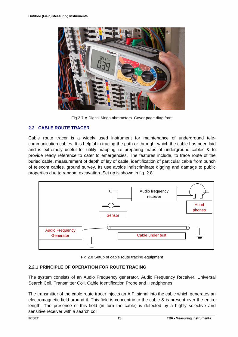
2.1.3 Digital Insulation Tester Handling measurements for testing on telecommunications systems and electronic equipment
the Digital Mega ohmmeters are ideal. They offer test voltages of 50 V and 100 V or up to500 V
with low currents. To simplify measurements, it is also possible to program thresholds that
trigger a buzzer. Best suited for telecommunications and ideal for measurements on telephone
lines includes specific functions: resistance, capacitance, current and AC voltage measurement.
Some advanced models can be used to check the presence of transmission frames or to
measure the resistance difference between 2 wires and also directly displays the length in km of
the line being tested through programming of the capacitance per unit length in nF/km. A typical
Digital Mega ohmmeters is shown in fig 2.7.
Outdoor (Field) Measuring Instruments
IRISET 23 TB6 - Measuring instruments
Fig 2.7 A Digital Mega ohmmeters Cover page diag front
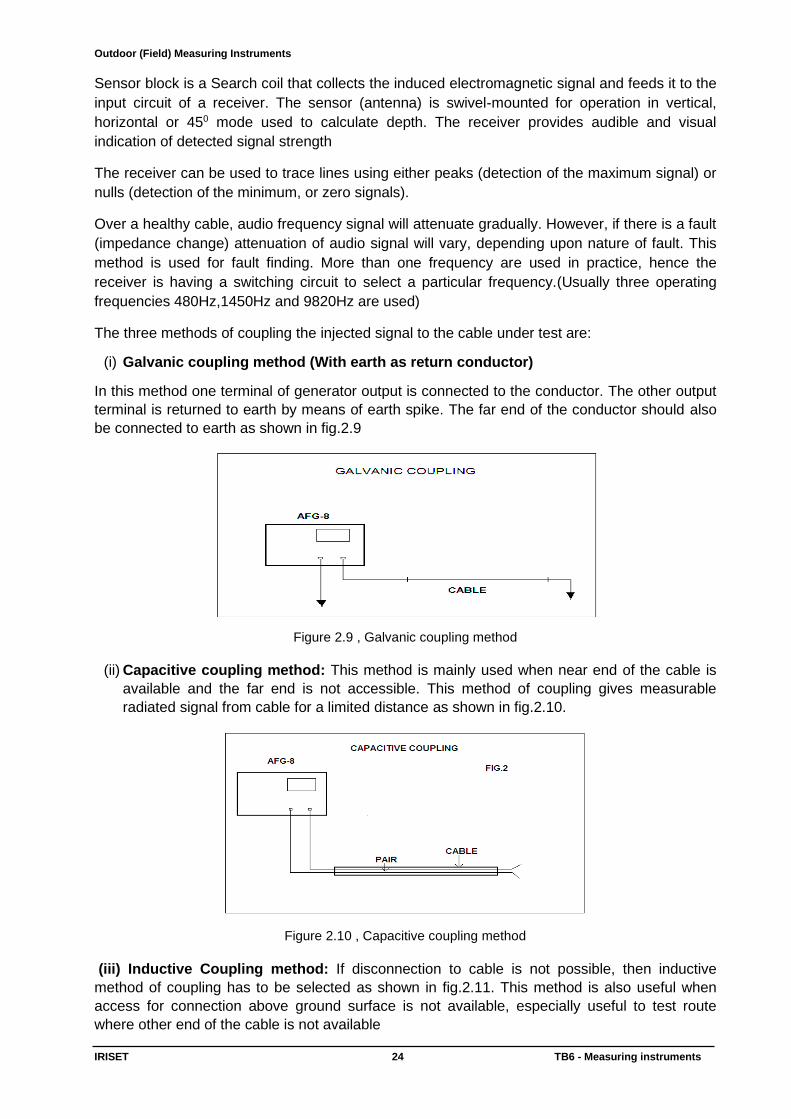
2.2 CABLE ROUTE TRACER Cable route tracer is a widely used instrument for maintenance of underground tele-
communication cables. It is helpful in tracing the path or through which the cable has been laid
and is extremely useful for utility mapping i.e preparing maps of underground cables & to
provide ready reference to cater to emergencies. The features include, to trace route of the
buried cable, measurement of depth of lay of cable, identification of particular cable from bunch
of telecom cables, ground survey. Its use avoids indiscriminate digging and damage to public
properties due to random excavation Set up is shown in fig. 2.8
Fig.2.8 Setup of cable route tracing equipment
2.2.1 PRINCIPLE OF OPERATION FOR ROUTE TRACING The system consists of an Audio Frequency generator, Audio Frequency Receiver, Universal
Search Coil, Transmitter Coil, Cable Identification Probe and Headphones
The transmitter of the cable route tracer injects an A.F. signal into the cable which generates an
electromagnetic field around it. This field is concentric to the cable & is present over the entire
length. The presence of this field (in turn the cable) is detected by a highly selective and
sensitive receiver with a search coil.
Audio Frequency
Generator
Audio frequency
receiver
Sensor
Cable under test
Head
phones
Outdoor (Field) Measuring Instruments
IRISET 24 TB6 - Measuring instruments
Sensor block is a Search coil that collects the induced electromagnetic signal and feeds it to the
input circuit of a receiver. The sensor (antenna) is swivel-mounted for operation in vertical,
horizontal or 450 mode used to calculate depth. The receiver provides audible and visual
indication of detected signal strength
The receiver can be used to trace lines using either peaks (detection of the maximum signal) or
nulls (detection of the minimum, or zero signals).
Over a healthy cable, audio frequency signal will attenuate gradually. However, if there is a fault
(impedance change) attenuation of audio signal will vary, depending upon nature of fault. This
method is used for fault finding. More than one frequency are used in practice, hence the
receiver is having a switching circuit to select a particular frequency.(Usually three operating
frequencies 480Hz,1450Hz and 9820Hz are used)
The three methods of coupling the injected signal to the cable under test are:
(i) Galvanic coupling method (With earth as return conductor)
In this method one terminal of generator output is connected to the conductor. The other output
terminal is returned to earth by means of earth spike. The far end of the conductor should also
be connected to earth as shown in fig.2.9
Figure 2.9 , Galvanic coupling method
(ii) Capacitive coupling method: This method is mainly used when near end of the cable is
available and the far end is not accessible. This method of coupling gives measurable
radiated signal from cable for a limited distance as shown in fig.2.10.
Figure 2.10 , Capacitive coupling method
(iii) Inductive Coupling method: If disconnection to cable is not possible, then inductive
method of coupling has to be selected as shown in fig.2.11. This method is also useful when
access for connection above ground surface is not available, especially useful to test route
where other end of the cable is not available
Outdoor (Field) Measuring Instruments
IRISET 25 TB6 - Measuring instruments
..
Figure 2.11 , Inductive Coupling method
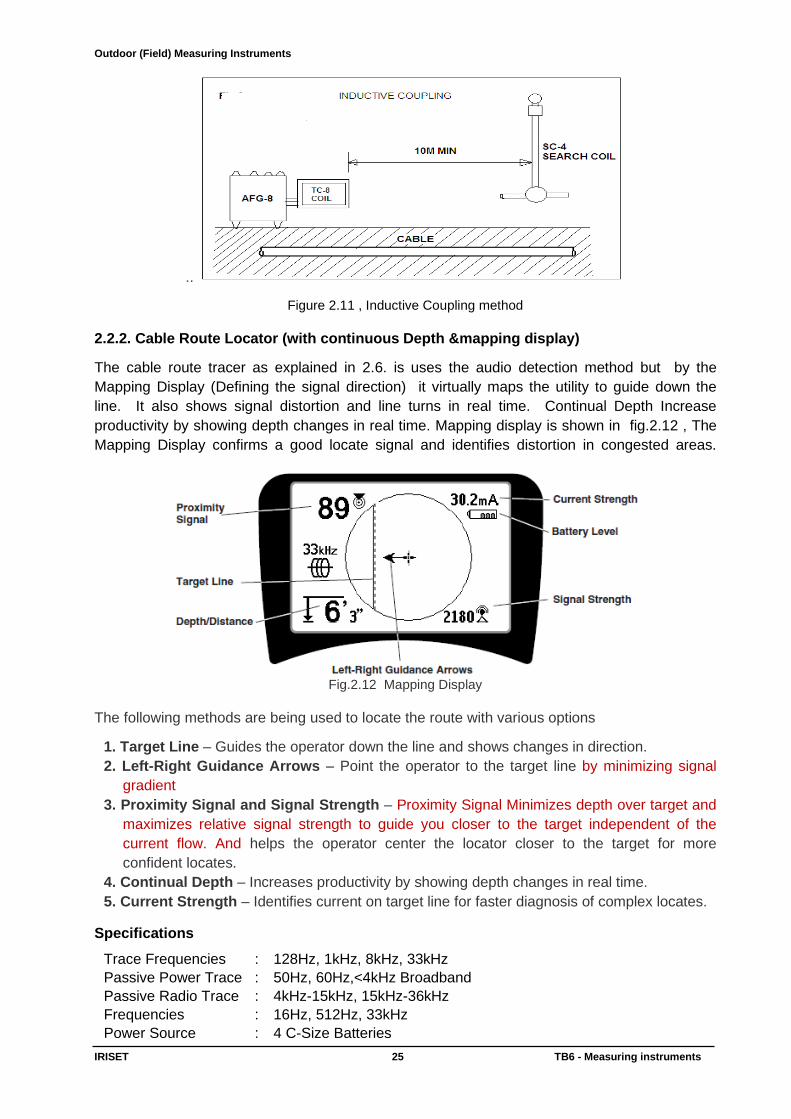
2.2.2. Cable Route Locator (with continuous Depth &mapping display)
The cable route tracer as explained in 2.6. is uses the audio detection method but by the
Mapping Display (Defining the signal direction) it virtually maps the utility to guide down the
line. It also shows signal distortion and line turns in real time. Continual Depth Increase
productivity by showing depth changes in real time. Mapping display is shown in fig.2.12 , The
Mapping Display confirms a good locate signal and identifies distortion in congested areas.
Fig.2.12 Mapping Display
The following methods are being used to locate the route with various options
1. Target Line – Guides the operator down the line and shows changes in direction.
2. Left-Right Guidance Arrows – Point the operator to the target line by minimizing signal
gradient
3. Proximity Signal and Signal Strength – Proximity Signal Minimizes depth over target and
maximizes relative signal strength to guide you closer to the target independent of the
current flow. And helps the operator center the locator closer to the target for more
confident locates.
4. Continual Depth – Increases productivity by showing depth changes in real time.
5. Current Strength – Identifies current on target line for faster diagnosis of complex locates.
Specifications
Trace Frequencies : 128Hz, 1kHz, 8kHz, 33kHz
Passive Power Trace : 50Hz, 60Hz,<4kHz Broadband
Passive Radio Trace : 4kHz-15kHz, 15kHz-36kHz
Frequencies : 16Hz, 512Hz, 33kHz
Power Source : 4 C-Size Batteries
Outdoor (Field) Measuring Instruments
IRISET 26 TB6 - Measuring instruments
2.3 CABLE FAULT LOCATOR A cable fault locator is used to mainly locate low insulation and contact faults in UG cables. This
instrument can also be used to measure distance to fault in case of clear open faults using
pulse reflection principles.
Cable Fault Locators are commonly used for in-place testing of very long cable runs, where it is
impractical to dig up or remove cable. They are indispensable for preventive maintenance of
telecommunication lines, as they can reveal growing resistance levels on joints and connectors
as they corrode, and increasing insulation leakage as it degrades and absorbs moisture long
before either leads to catastrophic failures. Using a cable fault locator, it is possible to pinpoint a
fault.
The different types of measurements used by a cable fault locator in U/G telecom cables are
following –
• To locate low insulation faults
• To detect open and short faults (distance of fault)
• For measuring insulation resistance
• For measuring foreign voltage on cables Cable Fault Locators are operated in two methods
1. Pulse Echo Method
2. Time Domain Reflectometer (TDR) 2.3.1 Pulse Echo Method: In this method, a low voltage short duration pulse is injected in the
cable and time taken by the pulse to travel to the point, where changes in insulation occur, and
the reflected back energy is measured. Limitation of this method is, only short circuit faults can
be located. It is essentially a high frequency AC pulsed signal generator that is used as a
source, and for fault localization pulse echo techniques is used. A defined pulse is transmitted
on the cable pair under test. The pulse travels along the pair length at a fixed velocity of
propagation depending on the dielectric of the cable. A part of the pulse energy reflects back
from the point where the characteristics impedance of cable changes due to fault occurrences.
The time taken by the pulse to reach the faulty location and return to the source multiplied by
the velocity of propagation gives twice the distance to fault. This is computed internally and
distance to fault is displayed directly in meters. The typical timing pulses are 80ns.250ns, 800ns
and 1800ns respectively for 0.3 KM, 1 KM, 3 KM and 10KM.
The faulty distance can be calculated by the formula- D= (V/2)T Where D= Distance to fault in meters
V= velocity of propagation
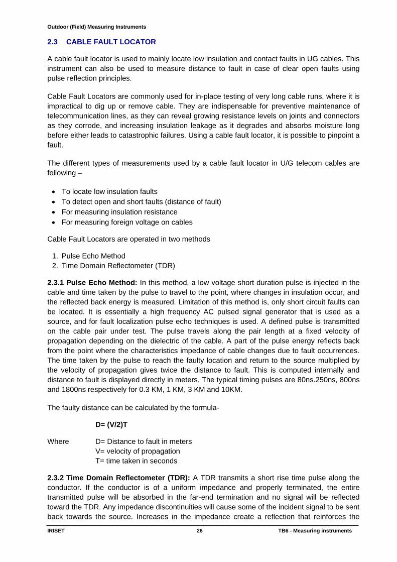
T= time taken in seconds 2.3.2 Time Domain Reflectometer (TDR): A TDR transmits a short rise time pulse along the
conductor. If the conductor is of a uniform impedance and properly terminated, the entire
transmitted pulse will be absorbed in the far-end termination and no signal will be reflected
toward the TDR. Any impedance discontinuities will cause some of the incident signal to be sent
back towards the source. Increases in the impedance create a reflection that reinforces the
Outdoor (Field) Measuring Instruments
IRISET 27 TB6 - Measuring instruments
original pulse whilst decreases in the impedance create a reflection that opposes the original
pulse. The resulting reflected pulse that is measured at the output/input to the TDR is displayed
or plotted as a function of time and, because the speed of signal propagation is almost constant
for a given transmission medium, can be read as a function of cable length. Because of this
sensitivity to impedance variations, a TDR may be used to verify cable impedance
characteristics .A typical Time Domain Reflectometer is shown in fig 2.13 .
Fig. 2,13, Time Domain Reflectometer
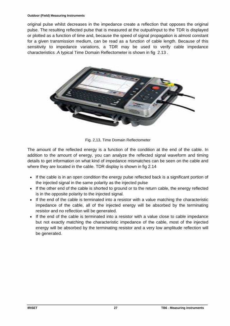
The amount of the reflected energy is a function of the condition at the end of the cable. In
addition to the amount of energy, you can analyze the reflected signal waveform and timing
details to get information on what kind of impedance mismatches can be seen on the cable and
where they are located in the cable. TDR display is shown in fig 2.14
• If the cable is in an open condition the energy pulse reflected back is a significant portion of
the injected signal in the same polarity as the injected pulse
• If the other end of the cable is shorted to ground or to the return cable, the energy reflected
is in the opposite polarity to the injected signal.
• If the end of the cable is terminated into a resistor with a value matching the characteristic
impedance of the cable, all of the injected energy will be absorbed by the terminating
resistor and no reflection will be generated.
• If the end of the cable is terminated into a resistor with a value close to cable impedance
but not exactly matching the characteristic impedance of the cable, most of the injected
energy will be absorbed by the terminating resistor and a very low amplitude reflection will
be generated.
Outdoor (Field) Measuring Instruments
IRISET 28 TB6 - Measuring instruments
Fig. 2.14 , TDR Display
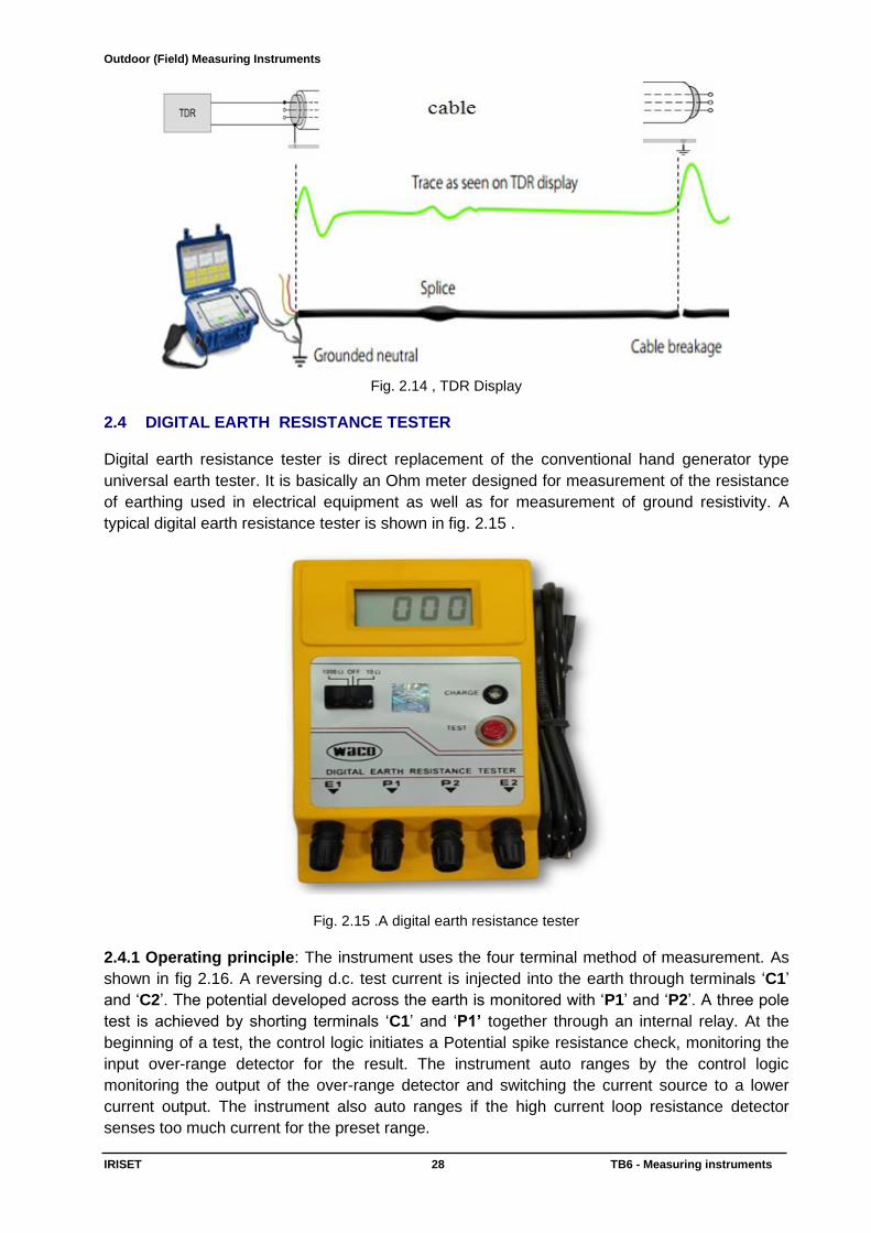
2.4 DIGITAL EARTH RESISTANCE TESTER Digital earth resistance tester is direct replacement of the conventional hand generator type
universal earth tester. It is basically an Ohm meter designed for measurement of the resistance
of earthing used in electrical equipment as well as for measurement of ground resistivity. A
typical digital earth resistance tester is shown in fig. 2.15 .
Fig. 2.15 .A digital earth resistance tester
2.4.1 Operating principle: The instrument uses the four terminal method of measurement. As
shown in fig 2.16. A reversing d.c. test current is injected into the earth through terminals ‘C1’
and ‘C2’. The potential developed across the earth is monitored with ‘P1’ and ‘P2’. A three pole
test is achieved by shorting terminals ‘C1’ and ‘P1’ together through an internal relay. At the
beginning of a test, the control logic initiates a Potential spike resistance check, monitoring the
input over-range detector for the result. The instrument auto ranges by the control logic
monitoring the output of the over-range detector and switching the current source to a lower
current output. The instrument also auto ranges if the high current loop resistance detector
senses too much current for the preset range.

Outdoor (Field) Measuring Instruments
IRISET 29 TB6 - Measuring instruments
C1
P2
C B
P1
D
M
A
C2
Fig 2.16 , Typical Block diagram of digital earth tester
The instrument measuring circuitry is connected to terminals ‘P1’ and ‘P2’. The voltage limiter
and input buffer prevent damage to the instrument and loading of the resistance under test.
Synchronous filtering and detection are used to recover the test signal from noisy environments
followed by filtering and conversion to a reading by the digital panel meter. The test signal
frequency is produced by dividing the frequency of a crystal oscillator. This is then passed
through logic circuitry to produce the waveforms for synchronous filtering and detection.
Four electrodes ABCD are rods driven in the earth, the resistance of which is to be tested at a
distance of 20m from each other as shown in fig.2.17
Fig.2.17 , Measuring of earth resistance using 4- electrode method
Outdoor (Field) Measuring Instruments
IRISET 30 TB6 - Measuring instruments
AC signal is applied to electrodes A and D and voltage developed across electrodes B and C
due to flow of current through the earth is measured by ammeter M. If the current is constant the
voltage measured will be directly proportional to the earth resistance.
To eliminate the error due to other signals, the meter reading will be sampled at the same
frequency as that of the applied signal. Accordingly the frequency selected is of an odd value
around 72Hz thus eliminating any chances of errors due to harmonics of 50Hz.
The sampling is done by having an FET across the meter and switching the FET at the selected
frequency only. The metering is also isolated from DC source.
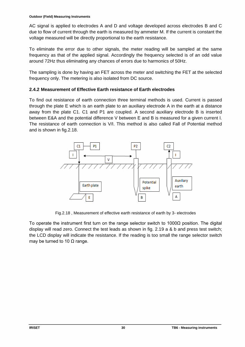
2.4.2 Measurement of Effective Earth resistance of Earth electrodes To find out resistance of earth connection three terminal methods is used. Current is passed
through the plate E which is an earth plate to an auxiliary electrode A in the earth at a distance
away from the plate C1. C1 and P1 are coupled. A second auxiliary electrode B is inserted
between E&A and the potential difference V between E and B is measured for a given current I.
The resistance of earth connection is V/I. This method is also called Fall of Potential method
and is shown in fig.2.18.
Fig.2.18 , Measurement of effective earth resistance of earth by 3- electrodes
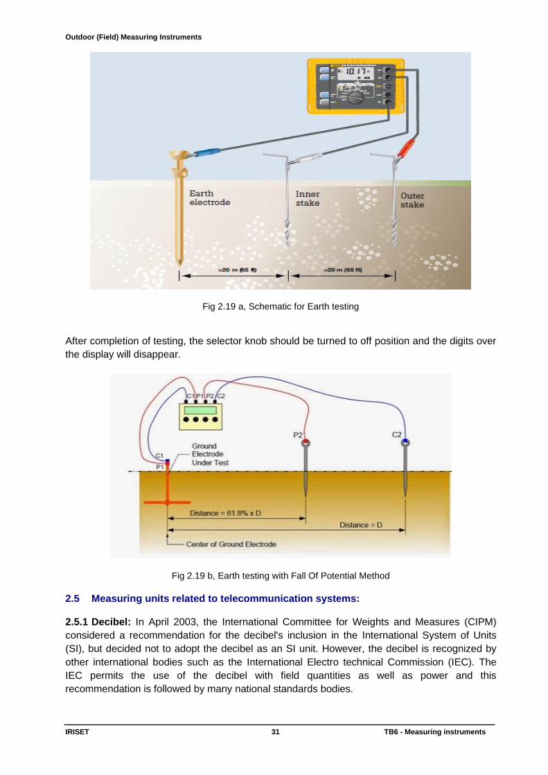
To operate the instrument first turn on the range selector switch to 1000Ω position. The digital
display will read zero. Connect the test leads as shown in fig. 2.19 a & b and press test switch;
the LCD display will indicate the resistance. If the reading is too small the range selector switch
may be turned to 10 Ω range.
Outdoor (Field) Measuring Instruments
IRISET 31 TB6 - Measuring instruments
Fig 2.19 a, Schematic for Earth testing
After completion of testing, the selector knob should be turned to off position and the digits over
the display will disappear.
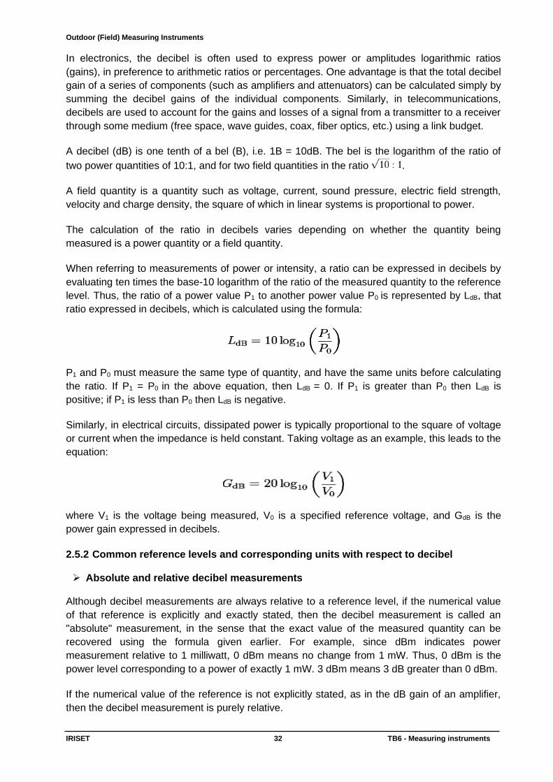
Fig 2.19 b, Earth testing with Fall Of Potential Method
2.5 Measuring units related to telecommunication systems: 2.5.1 Decibel: In April 2003, the International Committee for Weights and Measures (CIPM)
considered a recommendation for the decibel's inclusion in the International System of Units
(SI), but decided not to adopt the decibel as an SI unit. However, the decibel is recognized by
other international bodies such as the International Electro technical Commission (IEC). The
IEC permits the use of the decibel with field quantities as well as power and this
recommendation is followed by many national standards bodies.
Outdoor (Field) Measuring Instruments
IRISET 32 TB6 - Measuring instruments
In electronics, the decibel is often used to express power or amplitudes logarithmic ratios
(gains), in preference to arithmetic ratios or percentages. One advantage is that the total decibel
gain of a series of components (such as amplifiers and attenuators) can be calculated simply by
summing the decibel gains of the individual components. Similarly, in telecommunications,
decibels are used to account for the gains and losses of a signal from a transmitter to a receiver
through some medium (free space, wave guides, coax, fiber optics, etc.) using a link budget.
A decibel (dB) is one tenth of a bel (B), i.e. 1B = 10dB. The bel is the logarithm of the ratio of
two power quantities of 10:1, and for two field quantities in the ratio .
A field quantity is a quantity such as voltage, current, sound pressure, electric field strength,
velocity and charge density, the square of which in linear systems is proportional to power.
The calculation of the ratio in decibels varies depending on whether the quantity being
measured is a power quantity or a field quantity.
When referring to measurements of power or intensity, a ratio can be expressed in decibels by
evaluating ten times the base-10 logarithm of the ratio of the measured quantity to the reference
level. Thus, the ratio of a power value P1 to another power value P0 is represented by LdB, that
ratio expressed in decibels, which is calculated using the formula:
P1 and P0 must measure the same type of quantity, and have the same units before calculating
the ratio. If P1 = P0 in the above equation, then LdB = 0. If P1 is greater than P0 then LdB is
positive; if P1 is less than P0 then LdB is negative.
Similarly, in electrical circuits, dissipated power is typically proportional to the square of voltage
or current when the impedance is held constant. Taking voltage as an example, this leads to the
equation:
where V1 is the voltage being measured, V0 is a specified reference voltage, and GdB is the
power gain expressed in decibels.
2.5.2 Common reference levels and corresponding units with respect to decibel Absolute and relative decibel measurements
Although decibel measurements are always relative to a reference level, if the numerical value
of that reference is explicitly and exactly stated, then the decibel measurement is called an
"absolute" measurement, in the sense that the exact value of the measured quantity can be
recovered using the formula given earlier. For example, since dBm indicates power
measurement relative to 1 milliwatt, 0 dBm means no change from 1 mW. Thus, 0 dBm is the
power level corresponding to a power of exactly 1 mW. 3 dBm means 3 dB greater than 0 dBm.
If the numerical value of the reference is not explicitly stated, as in the dB gain of an amplifier,
then the decibel measurement is purely relative.
Outdoor (Field) Measuring Instruments
IRISET 33 TB6 - Measuring instruments
Absolute measurements Power dBm or dBmW: dB(1 mW) – power measurement relative to 1 milliwatt. X dBm = X dBW + 30. dBW: dB(1 W) – similar to dBm, except the reference level is 1 watt.
0 dBW = +30 dBm;
−30 dBW = 0 dBm;
XdBW = XdBm − 30. Voltage: Since the decibel is defined with respect to power not amplitude, conversions of
voltage ratios to decibels must square the amplitude
dBV: dB(1 VRMS) – voltage relative to 1 volt, regardless of impedance. dBu or dBv: dB(0.775 VRMS) – voltage relative to 0.775 volts. Originally dBv, it was changed
to dBu to avoid confusion with dBV. The "v" comes from "volt", while "u" comes from
"unloaded". dBu can be used regardless of impedance, but is derived from a 600 Ω load
dissipating 0 dBm (1 mW).
dBmV: dB(1 mVRMS) – voltage relative to 1 millivolt. Widely used in cable television networks,
where the nominal strength of a single TV signal at the receiver terminals is about 0 dBmV.
Cable TV uses 75 Ω coaxial cable, so 0 dBmV corresponds to −78.75 dBW (−48.75 dBm) or
~13 nW.
dBμV or dBuV: dB(1 μVRMS) – voltage relative to 1 microvolt. Widely used in television and
aerial amplifier specifications. 60 dBμV = 0 dBmV.
Radio power, energy and field strength dBc: relative to carrier—in telecommunications, this indicates the relative levels of noise or
sideband peak power, compared with the carrier power.
dB(J) – energy relative to 1 joule. 1 joule = 1 watt per hertz, so power spectral density can be
expressed in dBJ.
Antenna measurements dBi: dB(isotropic) – the forward gain of an antenna compared with the hypothetical isotropic
antenna, which uniformly distributes energy in all directions. Linear polarization of the EM field is
assumed unless noted otherwise.
dBd: dB(dipole) – the forward gain of an antenna compared with a half-wave dipole antenna. 0
dBd = 2.15 dBi
dBiC: dB(isotropic circular) – the forward gain of an antenna compared to a circularly polarized
isotropic antenna. There is no fixed conversion rule between dBiC and dBi, as it depends on the
receiving antenna and the field polarization.
dBq: dB(quarter wave) – the forward gain of an antenna compared to a quarter wavelength
whip. Rarely used, except in some marketing material. 0 dBq = −0.85 dBi
Outdoor (Field) Measuring Instruments
IRISET 34 TB6 - Measuring instruments
dBFS or dBfs: dB(full scale) – the amplitude of a signal (usually audio) compared with the
maximum which a device can handle before clipping occurs. In digital systems, 0 dBFS (peak)
would equal the highest level (number) the processor is capable of representing. Measured
values are always negative or zero, since they are less than the maximum or full-scale. Full-
scale is typically defined as the power level of a full-scale sinusoid, though some systems will
have extra headroom for peaks above the nominal full scale.
dB-Hz: dB(hertz) – bandwidth relative to 1 Hz. E.g., 20 dB-Hz corresponds to a bandwidth of
100 Hz. Commonly used in link budget calculations. Also used in carrier-to-noise-density ratio
(not to be confused with carrier-to-noise ratio, in dB).
dBov or dBO: dB(overload) – the amplitude of a signal (usually audio) compared with the
maximum which a device can handle before clipping occurs. Similar to dBFS, but also
applicable to analog systems.
dBr: dB(relative) – simply a relative difference from something else, which is made apparent in
context. The difference of a filter's response to nominal levels, for instance.
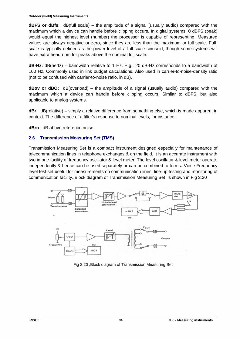
dBrn : dB above reference noise. 2.6 Transmission Measuring Set (TMS) Transmission Measuring Set is a compact instrument designed especially for maintenance of
telecommunication lines in telephone exchanges & on the field. It is an accurate instrument with
two in one facility of frequency oscillator & level meter. The level oscillator & level meter operate
independently & hence can be used separately or can be combined to form a Voice Frequency
level test set useful for measurements on communication lines, line-up testing and monitoring of
communication facility.,Block diagram of Transmission Measuring Set is shown in Fig 2.20
Fig 2.20 ,Block diagram of Transmission Measuring Set
Outdoor (Field) Measuring Instruments
IRISET 35 TB6 - Measuring instruments
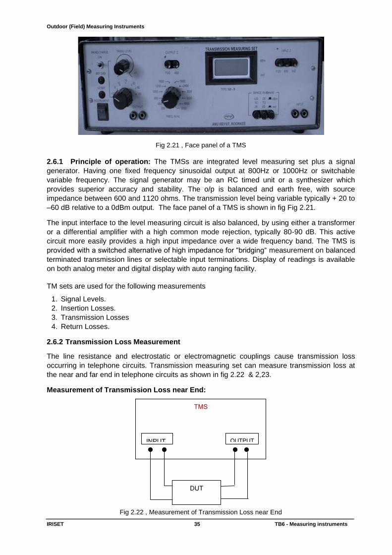
Fig 2.21 , Face panel of a TMS
2.6.1 Principle of operation: The TMSs are integrated level measuring set plus a signal
generator. Having one fixed frequency sinusoidal output at 800Hz or 1000Hz or switchable
variable frequency. The signal generator may be an RC timed unit or a synthesizer which
provides superior accuracy and stability. The o/p is balanced and earth free, with source
impedance between 600 and 1120 ohms. The transmission level being variable typically + 20 to
–60 dB relative to a 0dBm output. The face panel of a TMS is shown in fig Fig 2.21.
The input interface to the level measuring circuit is also balanced, by using either a transformer
or a differential amplifier with a high common mode rejection, typically 80-90 dB. This active
circuit more easily provides a high input impedance over a wide frequency band. The TMS is
provided with a switched alternative of high impedance for “bridging“ measurement on balanced
terminated transmission lines or selectable input terminations. Display of readings is available
on both analog meter and digital display with auto ranging facility.
TM sets are used for the following measurements
1. Signal Levels.
2. Insertion Losses.
3. Transmission Losses
4. Return Losses.
2.6.2 Transmission Loss Measurement
The line resistance and electrostatic or electromagnetic couplings cause transmission loss
occurring in telephone circuits. Transmission measuring set can measure transmission loss at
the near and far end in telephone circuits as shown in fig 2.22 & 2,23.
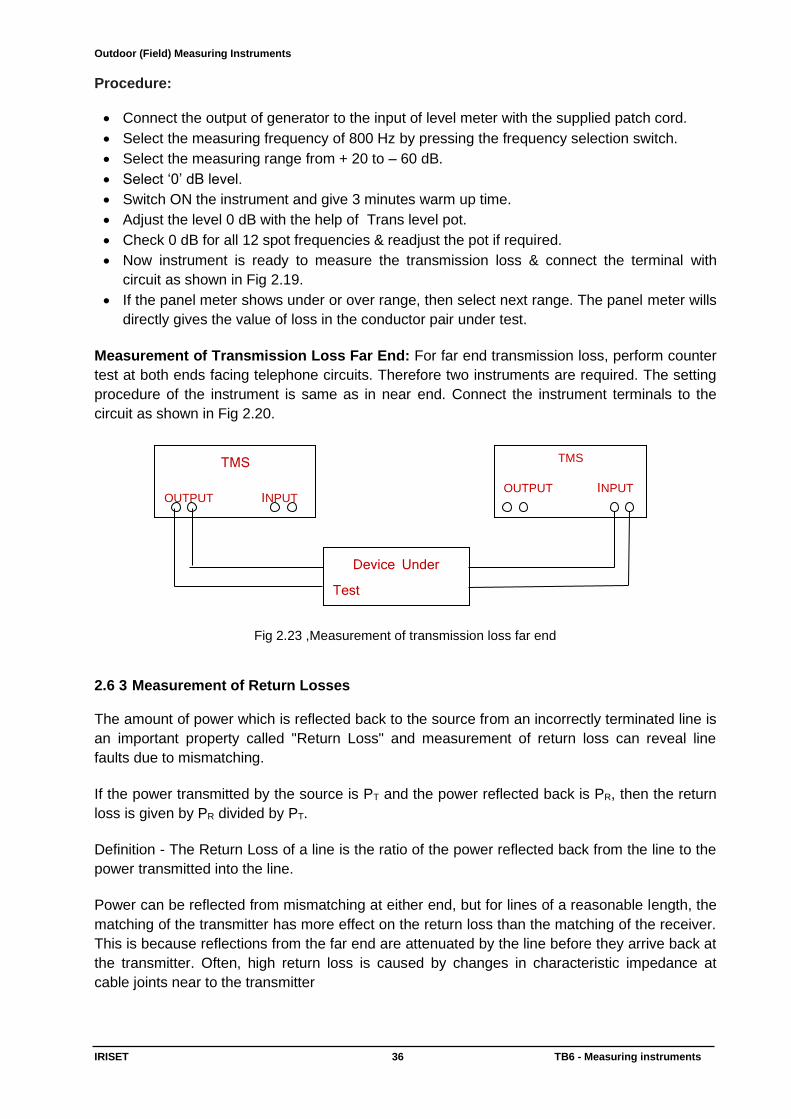
Measurement of Transmission Loss near End:
Fig 2.22 , Measurement of Transmission Loss near End
TMS
DUT
INPUT OUTPUT
Outdoor (Field) Measuring Instruments
IRISET 36 TB6 - Measuring instruments
Procedure:
• Connect the output of generator to the input of level meter with the supplied patch cord.
• Select the measuring frequency of 800 Hz by pressing the frequency selection switch.
• Select the measuring range from + 20 to – 60 dB.
• Select ‘0’ dB level.
• Switch ON the instrument and give 3 minutes warm up time.
• Adjust the level 0 dB with the help of Trans level pot.
• Check 0 dB for all 12 spot frequencies & readjust the pot if required.
• Now instrument is ready to measure the transmission loss & connect the terminal with
circuit as shown in Fig 2.19.
• If the panel meter shows under or over range, then select next range. The panel meter wills
directly gives the value of loss in the conductor pair under test.
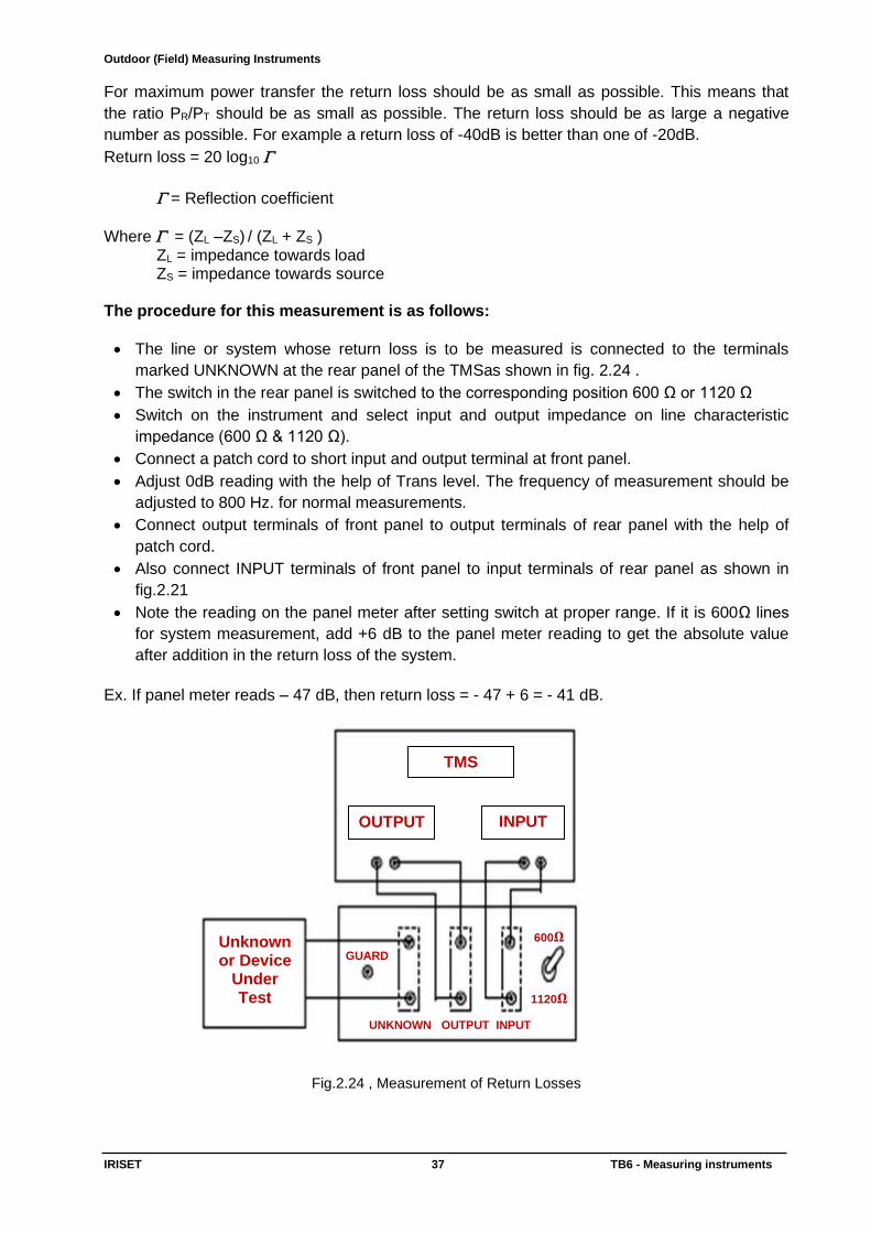
Measurement of Transmission Loss Far End: For far end transmission loss, perform counter
test at both ends facing telephone circuits. Therefore two instruments are required. The setting
procedure of the instrument is same as in near end. Connect the instrument terminals to the
circuit as shown in Fig 2.20.
Fig 2.23 ,Measurement of transmission loss far end
2.6 3 Measurement of Return Losses The amount of power which is reflected back to the source from an incorrectly terminated line is
an important property called "Return Loss" and measurement of return loss can reveal line
faults due to mismatching.
If the power transmitted by the source is PT and the power reflected back is PR, then the return
loss is given by PR divided by PT.
Definition - The Return Loss of a line is the ratio of the power reflected back from the line to the
power transmitted into the line.
Power can be reflected from mismatching at either end, but for lines of a reasonable length, the
matching of the transmitter has more effect on the return loss than the matching of the receiver.
This is because reflections from the far end are attenuated by the line before they arrive back at
the transmitter. Often, high return loss is caused by changes in characteristic impedance at
cable joints near to the transmitter
TMS
OUTPUT INPUT
TMS
OUTPUT INPUT
Device Under Test (DUT)
Outdoor (Field) Measuring Instruments
IRISET 37 TB6 - Measuring instruments
For maximum power transfer the return loss should be as small as possible. This means that
the ratio PR/PT should be as small as possible. The return loss should be as large a negative
number as possible. For example a return loss of -40dB is better than one of -20dB.
Return loss = 20 log10
= Reflection coefficient
Where = (ZL –ZS) / (ZL + ZS ) ZL = impedance towards load ZS = impedance towards source The procedure for this measurement is as follows:
• The line or system whose return loss is to be measured is connected to the terminals
marked UNKNOWN at the rear panel of the TMSas shown in fig. 2.24 .
• The switch in the rear panel is switched to the corresponding position 600 Ω or 1120 Ω
• Switch on the instrument and select input and output impedance on line characteristic
impedance (600 Ω & 1120 Ω).
• Connect a patch cord to short input and output terminal at front panel.
• Adjust 0dB reading with the help of Trans level. The frequency of measurement should be
adjusted to 800 Hz. for normal measurements.
• Connect output terminals of front panel to output terminals of rear panel with the help of
patch cord.
• Also connect INPUT terminals of front panel to input terminals of rear panel as shown in
fig.2.21
• Note the reading on the panel meter after setting switch at proper range. If it is 600Ω lines
for system measurement, add +6 dB to the panel meter reading to get the absolute value
after addition in the return loss of the system.
Ex. If panel meter reads – 47 dB, then return loss = - 47 + 6 = - 41 dB.
Fig.2.24 , Measurement of Return Losses
TMS
OUTPUT INPUT
Unknown or Device
Under Test
GUARD
600𝛀
1120𝛀
UNKNOWN OUTPUT INPUT
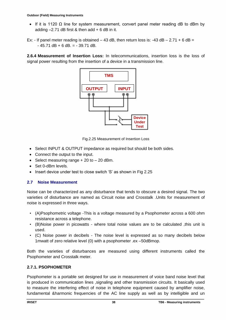
Outdoor (Field) Measuring Instruments
IRISET 38 TB6 - Measuring instruments
• If it is 1120 Ω line for system measurement, convert panel meter reading dB to dBm by
adding –2.71 dB first & then add + 6 dB in it.
Ex: - If panel meter reading is obtained – 43 dB, then return loss is: -43 dB – 2.71 + 6 dB =
- 45.71 dB + 6 dB. = - 39.71 dB.
2.6.4 Measurement of Insertion Loss: In telecommunications, insertion loss is the loss of
signal power resulting from the insertion of a device in a transmission line.
Fig.2.25 Measurement of Insertion Loss
• Select INPUT & OUTPUT impedance as required but should be both sides.
• Connect the output to the input.
• Select measuring range + 20 to – 20 dBm.
• Set 0-dBm levels.
• Insert device under test to close switch ‘S’ as shown in Fig 2.25
2.7 Noise Measurement Noise can be characterized as any disturbance that tends to obscure a desired signal. The two
varieties of disturbance are named as Circuit noise and Crosstalk .Units for measurement of
noise is expressed in three ways.
• (A)Psophometric voltage -This is a voltage measured by a Psophometer across a 600 ohm
resistance across a telephone.
• (B)Noise power in picowatts - where total noise values are to be calculated ,this unit is
used.
• (C) Noise power in decibels - The noise level is expressed as so many decibels below
1mwatt of zero relative level (0) with a psophometer .ex –50dBmop.
Both the varieties of disturbances are measured using different instruments called the
Psophometer and Crosstalk meter.
2.7.1. PSOPHOMETER Psophometer is a portable set designed for use in measurement of voice band noise level that
is produced in communication lines ,signaling and other transmission circuits. It basically used
to measure the interfering effect of noise in telephone equipment caused by amplifier noise,
fundamental &harmonic frequencies of the AC line supply as well as by intelligible and un
TMS
OUTPUT INPUT
Device Under Test
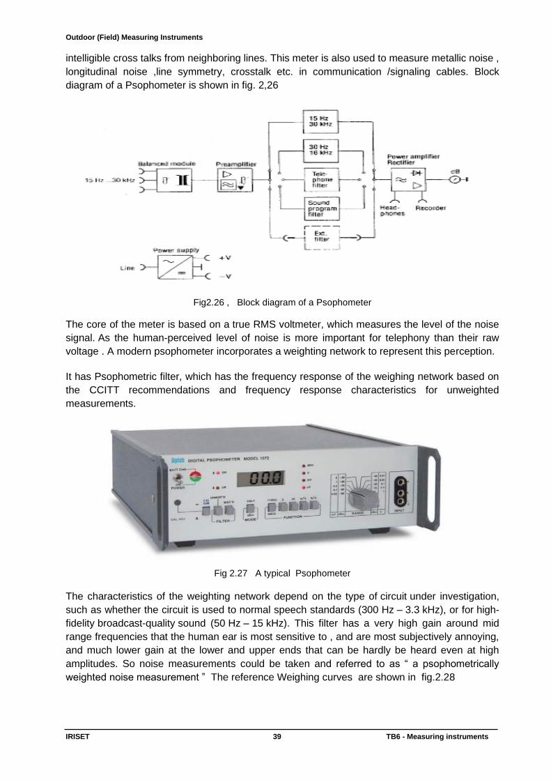
Outdoor (Field) Measuring Instruments
IRISET 39 TB6 - Measuring instruments
intelligible cross talks from neighboring lines. This meter is also used to measure metallic noise ,
longitudinal noise ,line symmetry, crosstalk etc. in communication /signaling cables. Block
diagram of a Psophometer is shown in fig. 2,26
Fig2.26 , Block diagram of a Psophometer
The core of the meter is based on a true RMS voltmeter, which measures the level of the noise
signal. As the human-perceived level of noise is more important for telephony than their raw
voltage . A modern psophometer incorporates a weighting network to represent this perception.
It has Psophometric filter, which has the frequency response of the weighing network based on
the CCITT recommendations and frequency response characteristics for unweighted
measurements.
Fig 2.27 A typical Psophometer
The characteristics of the weighting network depend on the type of circuit under investigation,
such as whether the circuit is used to normal speech standards (300 Hz – 3.3 kHz), or for high-
fidelity broadcast-quality sound (50 Hz – 15 kHz). This filter has a very high gain around mid
range frequencies that the human ear is most sensitive to , and are most subjectively annoying,
and much lower gain at the lower and upper ends that can be hardly be heard even at high
amplitudes. So noise measurements could be taken and referred to as “ a psophometrically
weighted noise measurement ” The reference Weighing curves are shown in fig.2.28
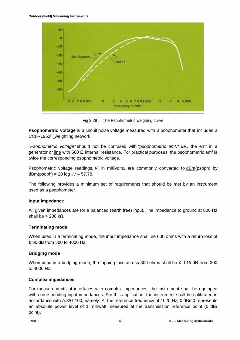
Outdoor (Field) Measuring Instruments
IRISET 40 TB6 - Measuring instruments
Fig 2.28 , The Psophometric weighing curve
Psophometric voltage is a circuit noise voltage measured with a psophometer that includes a
CCIF-1951[1] weighting network.
"Psophometric voltage" should not be confused with "psophometric emf," i.e., the emf in a
generator or line with 600 Ω internal resistance. For practical purposes, the psophometric emf is
twice the corresponding psophometric voltage.
Psophometric voltage readings, V, in millivolts, are commonly converted to dBm(psoph) by
dBm(psoph) = 20 log10V – 57.78.
The following provides a minimum set of requirements that should be met by an instrument
used as a psophometer.
Input impedance
All given impedances are for a balanced (earth free) input. The impedance to ground at 800 Hz
shall be > 200 kΩ.
Terminating mode
When used in a terminating mode, the input impedance shall be 600 ohms with a return loss of
≥ 30 dB from 300 to 4000 Hz.
Bridging mode
When used in a bridging mode, the tapping loss across 300 ohms shall be ≤ 0.15 dB from 300
to 4000 Hz.
Complex impedances
For measurements at interfaces with complex impedances, the instrument shall be equipped
with corresponding input impedances. For this application, the instrument shall be calibrated in
accordance with A.3/G.100, namely: At the reference frequency of 1020 Hz, 0 dBm0 represents
an absolute power level of 1 milliwatt measured at the transmission reference point (0 dBr
point).

Outdoor (Field) Measuring Instruments
IRISET 41 TB6 - Measuring instruments
Measuring range The usable measuring range of the instrument shall be –90 to 0 dBm. Calibration accuracy at 800 Hz The output indication shall be 0 dBm • 0.2 dB with an input signal of 0 dBm at 800 Hz. Relative gain versus frequency (frequency weighting) The required frequency weighting coefficients and accuracy limits at various frequencies are
given in the following technical specification .
Procedure for measuring noise: In general metallic noise measurements are made by connecting the circuit under test to input
terminals. Select the proper filter on filter switch operate the range from 0dBm level to down
wards till on scale meter indication is observed. The metallic noise level is the algebraic sum of
the indication of the dbm meter scale and the dbm range switch setting. One of the primary
function of the set is to measure weighted noise produced in telephone circuits such as metallic
noise and noise to ground i.e longitudinal noise .The weighted filter in this set designed to
match the characteristic by the CCITT recommendations. Following steps are shown in fig. 2.29.
1. Connect the telephone circuit under test to input terminals of the meter
2. Set the function switch to 600 ohms impedance
3. Set filter switch to WGT’D(weighted)
4. Operate the range switch from 0 dBm to minus levels till meter indication is observed.
5. Record the noise indicated on the meter in units either in dBm or mV.
Fig. 2.29 ,Measurement of Noise with a Psophometer
2.7.2. CROSSTALK METER
Crosstalk (XT) is a phenomenon by which a signal transmitted on one circuit or channel of a
transmission system creates an undesired effect in another circuit or channel.In other words
Cross talk is the bleeding or leakage of any signal or circuit, unintentionally effecting another
signal or circuit.
In structured cabling, crosstalk can refer to electromagnetic interference from one unshielded
twisted pair to another twisted pair, normally running in parallel .Crosstalk is usually caused by
undesired capacitive, inductive, or conductive coupling from one circuit, part of a circuit, or
channel, to another finally capacitive and inductive coupling are the reasons for generating
crosstalk. The front view and simplified circuit of a crosstalk meter is given in fig . 2.30 and
2.31

Outdoor (Field) Measuring Instruments
IRISET 42 TB6 - Measuring instruments
FIG.2.30 , Front view of Crosstalk meter
Fig2.31,.Simplified circuit of a crosstalk meter.
Near end crosstalk (NEXT)
Interference between two pairs in a cable measured at the same end of the cable as the
interfering transmitter.
Far end crosstalk (FEXT)
Interference between two pairs of a cable measured at the other end of the cable with respect to
the interfering transmitter.
Cross talk measuring set is a portable instrument which is capable of measuring cross talk in
the audio frequency range with a built-in AF generator and measuring detector. As the
measuring range starts from zero dB it can be conveniently used as a transmission measuring
set. With a measuring range from +10 to -80 dB is suitable for 470/600/1120 Ώ impedance.
A standard interrupted "tone" was formerly used as a source, but now a special warble oscillator
is employed. The signal is impressed on the disturbing circuit, and the amount transferred by
magnetic and electric coupling (and also by leakage) is detected in the receiver connected to
the disturbed circuit. This received amount is then compared with the original signal by the
switching arrangement shown. When the calibrated shunt is so adjusted that the sound heard
through the shunt and that heard over the disturbed line are equally loud, then the setting of the
shunt gives the crosstalk. One unit of crosstalk exists between two circuits when the current
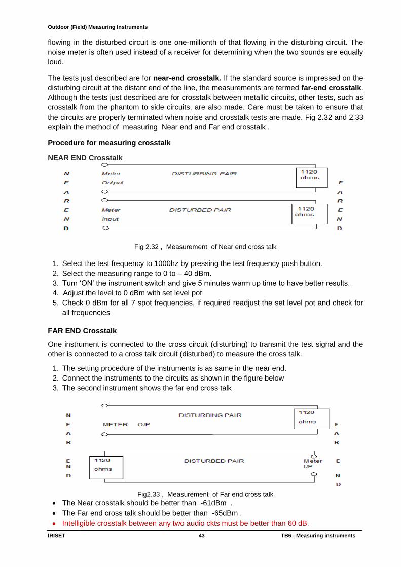
Outdoor (Field) Measuring Instruments
IRISET 43 TB6 - Measuring instruments
flowing in the disturbed circuit is one one-millionth of that flowing in the disturbing circuit. The
noise meter is often used instead of a receiver for determining when the two sounds are equally
loud.
The tests just described are for near-end crosstalk. If the standard source is impressed on the
disturbing circuit at the distant end of the line, the measurements are termed far-end crosstalk.
Although the tests just described are for crosstalk between metallic circuits, other tests, such as
crosstalk from the phantom to side circuits, are also made. Care must be taken to ensure that
the circuits are properly terminated when noise and crosstalk tests are made. Fig 2.32 and 2.33
explain the method of measuring Near end and Far end crosstalk .
Procedure for measuring crosstalk
NEAR END Crosstalk
Fig 2.32 , Measurement of Near end cross talk
1. Select the test frequency to 1000hz by pressing the test frequency push button.
2. Select the measuring range to 0 to – 40 dBm.
3. Turn ‘ON’ the instrument switch and give 5 minutes warm up time to have better results.
4. Adjust the level to 0 dBm with set level pot
5. Check 0 dBm for all 7 spot frequencies, if required readjust the set level pot and check for
all frequencies
FAR END Crosstalk
One instrument is connected to the cross circuit (disturbing) to transmit the test signal and the
other is connected to a cross talk circuit (disturbed) to measure the cross talk.
1. The setting procedure of the instruments is as same in the near end.
2. Connect the instruments to the circuits as shown in the figure below
3. The second instrument shows the far end cross talk
Fig2.33 , Measurement of Far end cross talk
• The Near crosstalk should be better than -61dBm .
• The Far end cross talk should be better than -65dBm .
• Intelligible crosstalk between any two audio ckts must be better than 60 dB.
Measuring Instruments used in OFC
IRISET 44 TB6 - Measuring instruments
CHAPTER-3
MEASURING INSTRUMENTS USED IN OFC 3.0 General Introduction Why and where we have to use OFC measurements?
• Link Certification
– Insertion loss
– Length
• Troubleshooting
– Equipment output power
– Link insertion loss
– Link continuity
– Link fault-locating The instruments which are mostly used in the field of OFC are
1. Visual Fault Locator
2. Optical power meter
3. OTDR 3.1 Visual Fault Locator Visual fault locator (also called laser fault locator) is a handheld device using 650nm or 635nm
visible laser source that emits a bright beam of laser light into a fiber, allowing the user to
visually detect a fiber fault for up to 5 km.
With these fault locators you can easily isolate high losses and faults in optical fiber cables. The
bright beam of 650nm or 635nm red light in a fiber allows you to see a break as a glowing or
blinking red light
They can operate on multimode or single mode fibers independent of the transmission
wavelength.
VFLs are designed to locate faults visually in single mode optical fiber cable
1. To locate breaks
2. To locate macro bends
3. To locate fault in connectors
4. To find end to end identification. These devices typically couple 1mW of 650nm Laser light into the fiber core, allowing for instant
identification of fiber breaks, micro or tight macro bending, even through tight buffered or un
buffered.
Two versions are available: one with a universal port for 2.5mm ferrule connectors and one
which includes an adapter that allows use with 1.25mm ferrule connectors
Applications include LAN, WAN, fiber data links, telephone and CATV.
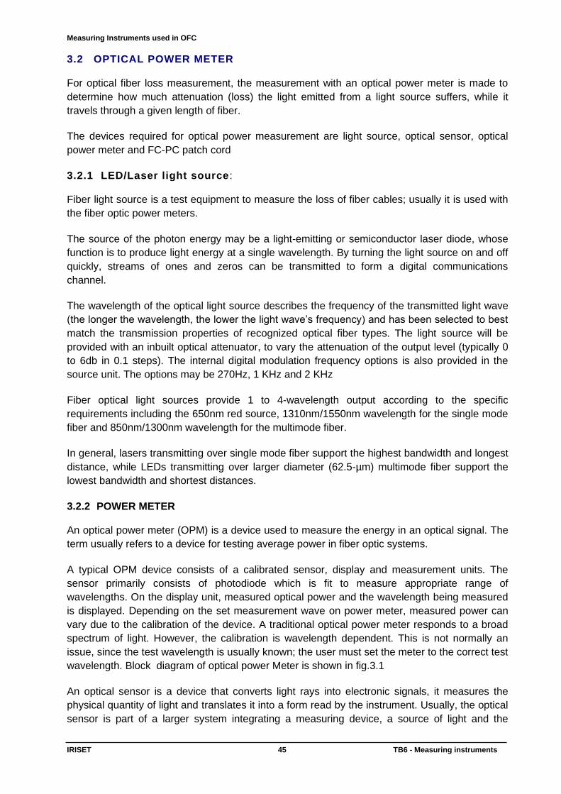
Measuring Instruments used in OFC
IRISET 45 TB6 - Measuring instruments
3.2 OPTICAL POWER METER For optical fiber loss measurement, the measurement with an optical power meter is made to
determine how much attenuation (loss) the light emitted from a light source suffers, while it
travels through a given length of fiber.
The devices required for optical power measurement are light source, optical sensor, optical
power meter and FC-PC patch cord
3.2.1 LED/Laser light source : Fiber light source is a test equipment to measure the loss of fiber cables; usually it is used with
the fiber optic power meters.
The source of the photon energy may be a light-emitting or semiconductor laser diode, whose
function is to produce light energy at a single wavelength. By turning the light source on and off
quickly, streams of ones and zeros can be transmitted to form a digital communications
channel.
The wavelength of the optical light source describes the frequency of the transmitted light wave
(the longer the wavelength, the lower the light wave’s frequency) and has been selected to best
match the transmission properties of recognized optical fiber types. The light source will be
provided with an inbuilt optical attenuator, to vary the attenuation of the output level (typically 0
to 6db in 0.1 steps). The internal digital modulation frequency options is also provided in the
source unit. The options may be 270Hz, 1 KHz and 2 KHz
Fiber optical light sources provide 1 to 4-wavelength output according to the specific
requirements including the 650nm red source, 1310nm/1550nm wavelength for the single mode
fiber and 850nm/1300nm wavelength for the multimode fiber.
In general, lasers transmitting over single mode fiber support the highest bandwidth and longest
distance, while LEDs transmitting over larger diameter (62.5-µm) multimode fiber support the
lowest bandwidth and shortest distances.
3.2.2 POWER METER An optical power meter (OPM) is a device used to measure the energy in an optical signal. The
term usually refers to a device for testing average power in fiber optic systems.
A typical OPM device consists of a calibrated sensor, display and measurement units. The
sensor primarily consists of photodiode which is fit to measure appropriate range of
wavelengths. On the display unit, measured optical power and the wavelength being measured
is displayed. Depending on the set measurement wave on power meter, measured power can
vary due to the calibration of the device. A traditional optical power meter responds to a broad
spectrum of light. However, the calibration is wavelength dependent. This is not normally an
issue, since the test wavelength is usually known; the user must set the meter to the correct test
wavelength. Block diagram of optical power Meter is shown in fig.3.1
An optical sensor is a device that converts light rays into electronic signals, it measures the
physical quantity of light and translates it into a form read by the instrument. Usually, the optical
sensor is part of a larger system integrating a measuring device, a source of light and the
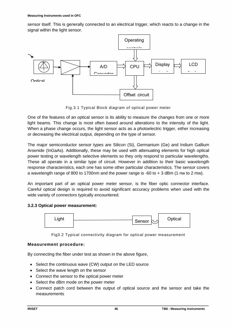
Measuring Instruments used in OFC
IRISET 46 TB6 - Measuring instruments
sensor itself. This is generally connected to an electrical trigger, which reacts to a change in the
signal within the light sensor.
Fig.3.1 Typical Block diagram of optical power meter
One of the features of an optical sensor is its ability to measure the changes from one or more
light beams. This change is most often based around alterations to the intensity of the light.
When a phase change occurs, the light sensor acts as a photoelectric trigger, either increasing
or decreasing the electrical output, depending on the type of sensor.
The major semiconductor sensor types are Silicon (Si), Germanium (Ge) and Indium Gallium
Arsenide (InGaAs). Additionally, these may be used with attenuating elements for high optical
power testing or wavelength selective elements so they only respond to particular wavelengths.
These all operate in a similar type of circuit. However in addition to their basic wavelength
response characteristics, each one has some other particular characteristics. The sensor covers
a wavelength range of 800 to 1700nm and the power range is -60 to + 3 dBm (1 nw to 2 mw).
An important part of an optical power meter sensor, is the fiber optic connector interface.
Careful optical design is required to avoid significant accuracy problems when used with the
wide variety of connectors typically encountered.
3.2.3 Optical power measurement:
Fig3.2 Typical connectivity diagram for optical power measurement
Measurement procedure: By connecting the fiber under test as shown in the above figure,
• Select the continuous wave (CW) output on the LED source
• Select the wave length on the sensor
• Connect the sensor to the optical power meter
• Select the dBm mode on the power meter
• Connect patch cord between the output of optical source and the sensor and take the
measurements
Sensor Optical power meter
Light source
under test
Operating controls
Offset circuit
A/D Converter
Display circuit
CPU LCD display
Optical sensor

Measuring Instruments used in OFC
IRISET 47 TB6 - Measuring instruments
3.3 OPTICAL TIME DOMAIN REFLECTOMETER (OTDR)
OTDR (Optical Time Domain Reflectometer) is a measuring instrument for identifying optic fiber
transmission features. The instrument is mainly used to measure attenuation of a whole optic
fiber chain and provide attenuation details relating to length namely to detect, locate and
measure any event in optic fiber chain (events refer to faults caused by splicing, connectors,
and bending whose transmission change can be measured). Its non-destructive one-end
connection and rapid measurement has made the OTDR an indispensable tool for manufacture,
construction, and maintenance of optic fiber.
Information relating to distance is obtained through time information (that’s the reason why there
is “time Domain” in the name of OTDR). Fresnel reflection occurs at the boundary between two
media of different (IOR) Index Of Refraction (for example, connections of faults, connectors, or
optic fiber end). This reflection is used to locate the discontinuous points on optic fiber. The
magnitude of reflection depends on the difference between IOR and the smoothness of
boundary.
The OTDR measures the time difference between the outgoing pulse and the incoming back
scattered pulses. An OTDR sends short pulses of light into a fiber. Light scattering occurs in the
fiber due to discontinuities such as connectors, splices, bends and faults. An OTDR then
detects and analyzes the backscattered signals. The signal strength is measured for specific
intervals of time and is used to characterize events. This way OTDR can be characterized
similar to optical radar. Block diagram of a OTDR is shown in fig. 3.3 .
An OTDR uses the effects of Rayleigh scattering and Fresnel reflection to measure the fiber
condition, but the Fresnel reflection is tens of thousands of times greater in power level than the
backscatter.
Rayleigh scattering occurs when a pulse travels down the fiber and small variations in the
material, such as variations and discontinuities in the index of refraction, cause light to be
scattered in all directions. However, the phenomenon of small amounts of light being reflected
directly back toward the transmitter is called backscattering.
Fresnel reflections occur when the light traveling down the fiber encounters abrupt changes in
material density that may occur at connections or breaks where an air gap exists. A very large
quantity of light is reflected, as compared with the Rayleigh scattering. The strength of the
reflection depends on the degree of change in the index of refraction. Fresnel reflections are
only point events.
Fig.3.3 Typical block diagram of an OTDR
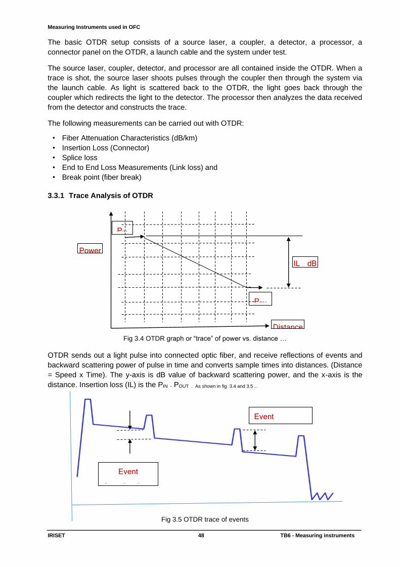
Measuring Instruments used in OFC
IRISET 48 TB6 - Measuring instruments
The basic OTDR setup consists of a source laser, a coupler, a detector, a processor, a
connector panel on the OTDR, a launch cable and the system under test.
The source laser, coupler, detector, and processor are all contained inside the OTDR. When a
trace is shot, the source laser shoots pulses through the coupler then through the system via
the launch cable. As light is scattered back to the OTDR, the light goes back through the
coupler which redirects the light to the detector. The processor then analyzes the data received
from the detector and constructs the trace.
The following measurements can be carried out with OTDR:
• Fiber Attenuation Characteristics (dB/km)
• Insertion Loss (Connector)
• Splice loss
• End to End Loss Measurements (Link loss) and
• Break point (fiber break)
3.3.1 Trace Analysis of OTDR
Fig 3.4 OTDR graph or “trace” of power vs. distance …
OTDR sends out a light pulse into connected optic fiber, and receive reflections of events and
backward scattering power of pulse in time and converts sample times into distances. (Distance
= Speed x Time). The y-axis is dB value of backward scattering power, and the x-axis is the
distance. Insertion loss (IL) is the PIN - POUT . As shown in fig 3.4 and 3.5 ..
Fig 3.5 OTDR trace of events
PIN
POU
T
IL dB
Distance
Power
Event insertion loss
Event reflectance
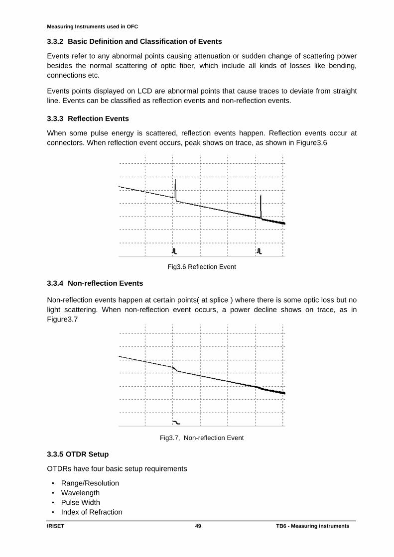
Measuring Instruments used in OFC
IRISET 49 TB6 - Measuring instruments
3.3.2 Basic Definition and Classification of Events
Events refer to any abnormal points causing attenuation or sudden change of scattering power
besides the normal scattering of optic fiber, which include all kinds of losses like bending,
connections etc.
Events points displayed on LCD are abnormal points that cause traces to deviate from straight
line. Events can be classified as reflection events and non-reflection events.
3.3.3 Reflection Events
When some pulse energy is scattered, reflection events happen. Reflection events occur at
connectors. When reflection event occurs, peak shows on trace, as shown in Figure3.6
Fig3.6 Reflection Event
3.3.4 Non-reflection Events Non-reflection events happen at certain points( at splice ) where there is some optic loss but no
light scattering. When non-reflection event occurs, a power decline shows on trace, as in
Figure3.7
Fig3.7, Non-reflection Event
3.3.5 OTDR Setup
OTDRs have four basic setup requirements
• Range/Resolution
• Wavelength
• Pulse Width
• Index of Refraction
Measuring Instruments used in OFC
IRISET 50 TB6 - Measuring instruments
Range is the selection of distance of fiber to be tested. Distance range will be typically 18, 36,
72,144 Km. In the horizontal axis (X- axis ) of the trace will be Km/full scale.
Wavelength selection is depending upon requirement as 1310 nm or 1550nm. The selected
wave length will be displayed on LCD.
Pulse Width is the width of the optical pulse from the OTDR reflected in a time frame. Long
pulse widths are suitable for long distance measurements but then the dead zone will become
wider and the connector for short intervals will disappear. On the other hand, short pulse widths
can identify connectors of short intervals but it cannot make long distance measurements as the
optical power will decrease. Pulse width will be expressed in µ seconds.
Index of Refraction enables the refractive index of the optical fiber to be set. The index range
will be 1.4000 to 1.5999 in 0.0001 steps.
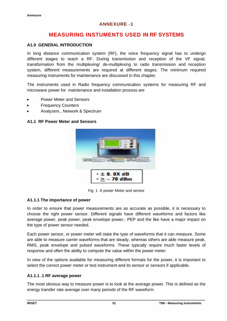
Annexure
IRISET 51 TB6 - Measuring instruments
ANNEXURE -1
MEASURING INSTUMENTS USED IN RF SYSTEMS A1.0 GENERAL INTRODUCTION
In long distance communication system (RF), the voice frequency signal has to undergo
different stages to reach a RF. During transmission and reception of the VF signal,
transformation from the multiplexing/ de-multiplexing to radio transmission and reception
system, different measurements are required at different stages. The minimum required
measuring instruments for maintenance are discussed in this chapter.
The instruments used in Radio frequency communication systems for measuring RF and
microwave power for maintenance and installation process are
• Power Meter and Sensors
• Frequency Counters
• Analyzers , Network & Spectrum
A1.1 RF Power Meter and Sensors
Fig 1 A power Meter and sensor
A1.1.1 The importance of power
In order to ensure that power measurements are as accurate as possible, it is necessary to
choose the right power sensor. Different signals have different waveforms and factors like
average power, peak power, peak envelope power,- PEP and the like have a major impact on
the type of power sensor needed.
Each power sensor, or power meter will state the type of waveforms that it can measure. Some
are able to measure carrier waveforms that are steady, whereas others are able measure peak,
RMS, peak envelope and pulsed waveforms. These typically require much faster levels of
response and often the ability to compute the value within the power meter.
In view of the options available for measuring different formats for the power, it is important to
select the correct power meter or test instrument and its sensor or sensors if applicable.
A1.1.1 .1 RF average power
The most obvious way to measure power is to look at the average power. This is defined as the
energy transfer rate average over many periods of the RF waveform.
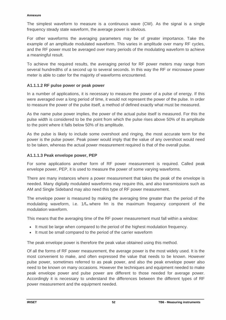
Annexure
IRISET 52 TB6 - Measuring instruments
The simplest waveform to measure is a continuous wave (CW). As the signal is a single
frequency steady state waveform, the average power is obvious.
For other waveforms the averaging parameters may be of greater importance. Take the
example of an amplitude modulated waveform. This varies in amplitude over many RF cycles,
and the RF power must be averaged over many periods of the modulating waveform to achieve
a meaningful result.
To achieve the required results, the averaging period for RF power meters may range from
several hundredths of a second up to several seconds. In this way the RF or microwave power
meter is able to cater for the majority of waveforms encountered.
A1.1.1.2 RF pulse power or peak power
In a number of applications, it is necessary to measure the power of a pulse of energy. If this
were averaged over a long period of time, it would not represent the power of the pulse. In order
to measure the power of the pulse itself, a method of defined exactly what must be measured.
As the name pulse power implies, the power of the actual pulse itself is measured. For this the
pulse width is considered to be the point from which the pulse rises above 50% of its amplitude
to the point where it falls below 50% of its amplitude.
As the pulse is likely to include some overshoot and ringing, the most accurate term for the
power is the pulse power. Peak power would imply that the value of any overshoot would need
to be taken, whereas the actual power measurement required is that of the overall pulse.
A1.1.1.3 Peak envelope power, PEP
For some applications another form of RF power measurement is required. Called peak
envelope power, PEP, it is used to measure the power of some varying waveforms.
There are many instances where a power measurement that takes the peak of the envelope is
needed. Many digitally modulated waveforms may require this, and also transmissions such as
AM and Single Sideband may also need this type of RF power measurement.
The envelope power is measured by making the averaging time greater than the period of the
modulating waveform, i.e. 1/fm where fm is the maximum frequency component of the
modulation waveform.
This means that the averaging time of the RF power measurement must fall within a window:
• It must be large when compared to the period of the highest modulation frequency.
• It must be small compared to the period of the carrier waveform
The peak envelope power is therefore the peak value obtained using this method.
Of all the forms of RF power measurement, the average power is the most widely used. It is the
most convenient to make, and often expressed the value that needs to be known. However
pulse power, sometimes referred to as peak power, and also the peak envelope power also
need to be known on many occasions. However the techniques and equipment needed to make
peak envelope power and pulse power are different to those needed for average power.
Accordingly it is necessary to understand the differences between the different types of RF
power measurement and the equipment needed.
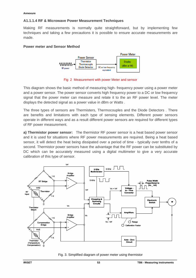
Annexure
IRISET 53 TB6 - Measuring instruments
A1.1.1.4 RF & Microwave Power Measurement Techniques
Making RF measurements is normally quite straightforward, but by implementing few
techniques and taking a few precautions it is possible to ensure accurate measurements are
made.
Power meter and Sensor Method
Fig 2 Measurement with power Meter and sensor
This diagram shows the basic method of measuring high- frequency power using a power meter
and a power sensor. The power sensor converts high frequency power to a DC or low frequency
signal that the power meter can measure and relate it to the an RF power level. The meter
displays the detected signal as a power value in dBm or Watts .
The three types of sensors are Thermisters, Thermocouples and the Diode Detectors . There
are benefits and limitations with each type of sensing elements. Different power sensors
operate in different ways and as a result different power sensors are required for different types
of RF power measurement.
a) Thermistor power sensor: The thermistor RF power sensor is a heat based power sensor
and it is used for situations where RF power measurements are required. Being a heat based
sensor, it will detect the heat being dissipated over a period of time - typically over tenths of a
second. Thermistor power sensors have the advantage that the RF power can be substituted by
DC which can be accurately measured using a digital multimeter to give a very accurate
calibration of this type of sensor.
Fig. 3. Simplified diagram of power meter using thermistor
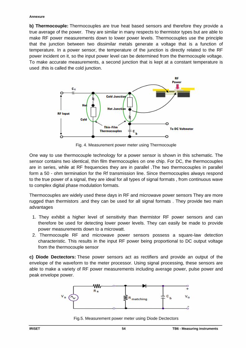
Annexure
IRISET 54 TB6 - Measuring instruments
b) Thermocouple: Thermocouples are true heat based sensors and therefore they provide a
true average of the power. They are similar in many respects to thermistor types but are able to
make RF power measurements down to lower power levels. Thermocouples use the principle
that the junction between two dissimilar metals generate a voltage that is a function of
temperature. In a power sensor, the temperature of the junction is directly related to the RF
power incident on it, so the input power level can be determined from the thermocouple voltage.
To make accurate measurements, a second junction that is kept at a constant temperature is
used .this is called the cold junction.
Fig. 4. Measurement power meter using Thermocouple
One way to use thermocouple technology for a power sensor is shown in this schematic. The
sensor contains two identical, thin film thermocouples on one chip. For DC, the thermocouples
are in series, while at RF frequencies they are in parallel .The two thermocouples in parallel
form a 50 - ohm termination for the Rf transmission line. Since thermocouples always respond
to the true power of a signal, they are ideal for all types of signal formats , from continuous wave
to complex digital phase modulation formats.
Thermocouples are widely used these days in RF and microwave power sensors They are more
rugged than thermistors .and they can be used for all signal formats . They provide two main
advantages
1. They exhibit a higher level of sensitivity than thermistor RF power sensors and can
therefore be used for detecting lower power levels. They can easily be made to provide
power measurements down to a microwatt.
2. Thermocouple RF and microwave power sensors possess a square-law detection
characteristic. This results in the input RF power being proportional to DC output voltage
from the thermocouple sensor
c) Diode Dectectors: These power sensors act as rectifiers and provide an output of the
envelope of the waveform to the meter processor. Using signal processing, these sensors are
able to make a variety of RF power measurements including average power, pulse power and
peak envelope power.
Fig.5. Measurement power meter using Diode Dectectors
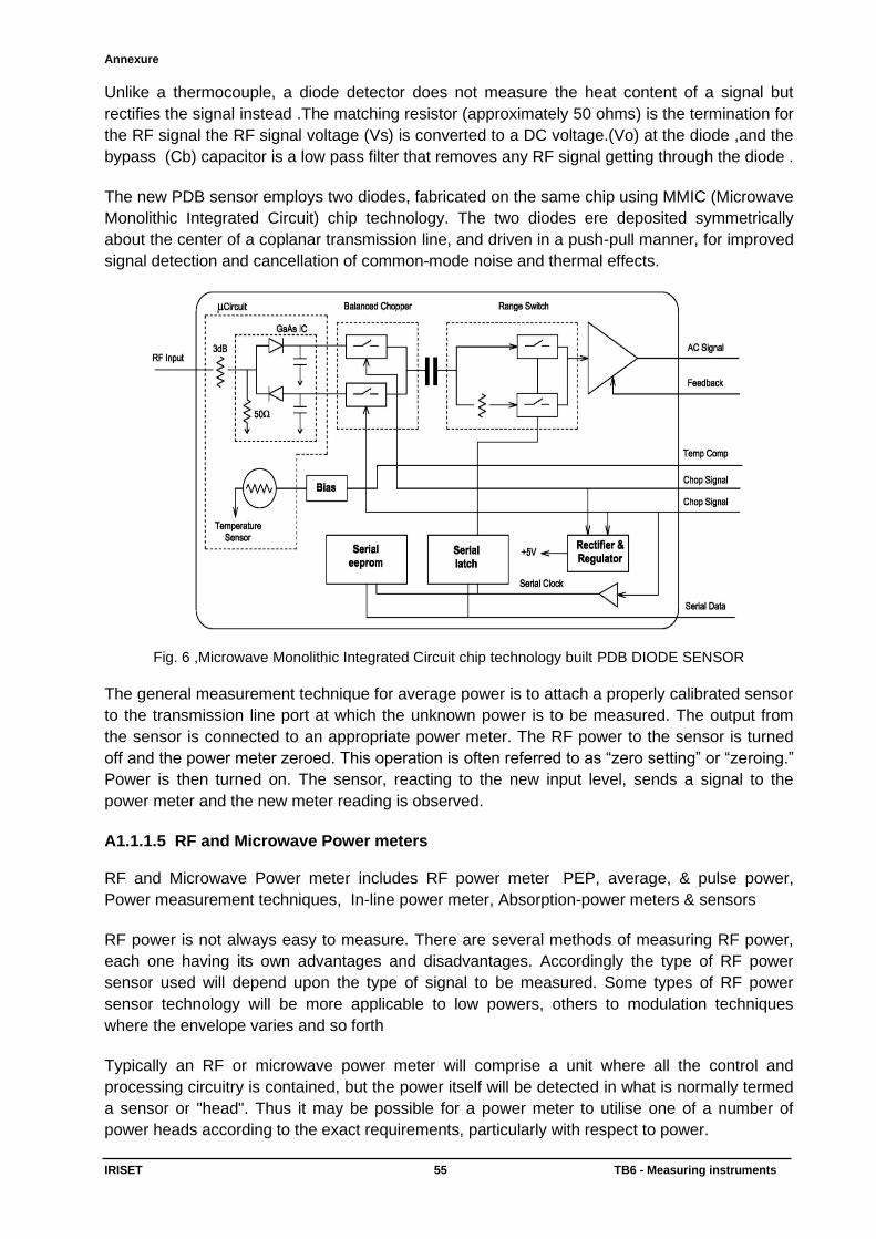
Annexure
IRISET 55 TB6 - Measuring instruments
Unlike a thermocouple, a diode detector does not measure the heat content of a signal but
rectifies the signal instead .The matching resistor (approximately 50 ohms) is the termination for
the RF signal the RF signal voltage (Vs) is converted to a DC voltage.(Vo) at the diode ,and the
bypass (Cb) capacitor is a low pass filter that removes any RF signal getting through the diode .
The new PDB sensor employs two diodes, fabricated on the same chip using MMIC (Microwave
Monolithic Integrated Circuit) chip technology. The two diodes ere deposited symmetrically
about the center of a coplanar transmission line, and driven in a push-pull manner, for improved
signal detection and cancellation of common-mode noise and thermal effects.
Fig. 6 ,Microwave Monolithic Integrated Circuit chip technology built PDB DIODE SENSOR
The general measurement technique for average power is to attach a properly calibrated sensor
to the transmission line port at which the unknown power is to be measured. The output from
the sensor is connected to an appropriate power meter. The RF power to the sensor is turned
off and the power meter zeroed. This operation is often referred to as “zero setting” or “zeroing.”
Power is then turned on. The sensor, reacting to the new input level, sends a signal to the
power meter and the new meter reading is observed.
A1.1.1.5 RF and Microwave Power meters RF and Microwave Power meter includes RF power meter PEP, average, & pulse power,
Power measurement techniques, In-line power meter, Absorption-power meters & sensors
RF power is not always easy to measure. There are several methods of measuring RF power,
each one having its own advantages and disadvantages. Accordingly the type of RF power
sensor used will depend upon the type of signal to be measured. Some types of RF power
sensor technology will be more applicable to low powers, others to modulation techniques
where the envelope varies and so forth
Typically an RF or microwave power meter will comprise a unit where all the control and
processing circuitry is contained, but the power itself will be detected in what is normally termed
a sensor or "head". Thus it may be possible for a power meter to utilise one of a number of
power heads according to the exact requirements, particularly with respect to power.
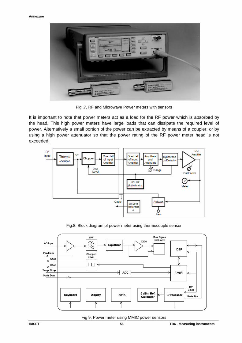
Annexure
IRISET 56 TB6 - Measuring instruments
Fig .7, RF and Microwave Power meters with sensors
It is important to note that power meters act as a load for the RF power which is absorbed by
the head. This high power meters have large loads that can dissipate the required level of
power. Alternatively a small portion of the power can be extracted by means of a coupler, or by
using a high power attenuator so that the power rating of the RF power meter head is not
exceeded.
Fig.8. Block diagram of power meter using thermocouple sensor
Fig 9, Power meter using MMIC power sensors
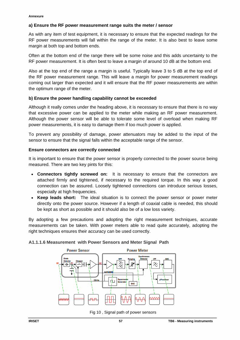
Annexure
IRISET 57 TB6 - Measuring instruments
a) Ensure the RF power measurement range suits the meter / sensor
As with any item of test equipment, it is necessary to ensure that the expected readings for the
RF power measurements will fall within the range of the meter. It is also best to leave some
margin at both top and bottom ends.
Often at the bottom end of the range there will be some noise and this adds uncertainty to the
RF power measurement. It is often best to leave a margin of around 10 dB at the bottom end.
Also at the top end of the range a margin is useful. Typically leave 3 to 5 dB at the top end of
the RF power measurement range. This will leave a margin for power measurement readings
coming out larger than expected and it will ensure that the RF power measurements are within
the optimum range of the meter.
b) Ensure the power handling capability cannot be exceeded
Although it really comes under the heading above, it is necessary to ensure that there is no way
that excessive power can be applied to the meter while making an RF power measurement.
Although the power sensor will be able to tolerate some level of overload when making RF
power measurements, it is easy to damage them if too much power is applied.
To prevent any possibility of damage, power attenuators may be added to the input of the
sensor to ensure that the signal falls within the acceptable range of the sensor.
Ensure connectors are correctly connected
It is important to ensure that the power sensor is properly connected to the power source being
measured. There are two key pints for this:
• Connectors tightly screwed on: It is necessary to ensure that the connectors are
attached firmly and tightened, if necessary to the required torque. In this way a good
connection can be assured. Loosely tightened connections can introduce serious losses,
especially at high frequencies.
• Keep leads short: The ideal situation is to connect the power sensor or power meter
directly onto the power source. However if a length of coaxial cable is needed, this should
be kept as short as possible and it should also be of a low loss variety.
By adopting a few precautions and adopting the right measurement techniques, accurate
measurements can be taken. With power meters able to read quite accurately, adopting the
right techniques ensures their accuracy can be used correctly.
A1.1.1.6 Measurement with Power Sensors and Meter Signal Path
Fig 10 , Signal path of power sensors
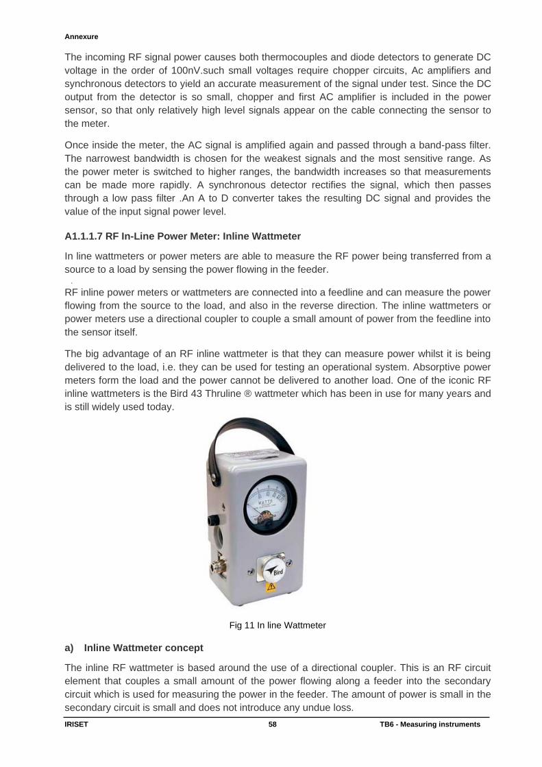
Annexure
IRISET 58 TB6 - Measuring instruments
The incoming RF signal power causes both thermocouples and diode detectors to generate DC
voltage in the order of 100nV.such small voltages require chopper circuits, Ac amplifiers and
synchronous detectors to yield an accurate measurement of the signal under test. Since the DC
output from the detector is so small, chopper and first AC amplifier is included in the power
sensor, so that only relatively high level signals appear on the cable connecting the sensor to
the meter.
Once inside the meter, the AC signal is amplified again and passed through a band-pass filter.
The narrowest bandwidth is chosen for the weakest signals and the most sensitive range. As
the power meter is switched to higher ranges, the bandwidth increases so that measurements
can be made more rapidly. A synchronous detector rectifies the signal, which then passes
through a low pass filter .An A to D converter takes the resulting DC signal and provides the
value of the input signal power level.
A1.1.1.7 RF In-Line Power Meter: Inline Wattmeter
In line wattmeters or power meters are able to measure the RF power being transferred from a
source to a load by sensing the power flowing in the feeder. .
RF inline power meters or wattmeters are connected into a feedline and can measure the power
flowing from the source to the load, and also in the reverse direction. The inline wattmeters or
power meters use a directional coupler to couple a small amount of power from the feedline into
the sensor itself.
The big advantage of an RF inline wattmeter is that they can measure power whilst it is being
delivered to the load, i.e. they can be used for testing an operational system. Absorptive power
meters form the load and the power cannot be delivered to another load. One of the iconic RF
inline wattmeters is the Bird 43 Thruline ® wattmeter which has been in use for many years and
is still widely used today.
Fig 11 In line Wattmeter
a) Inline Wattmeter concept
The inline RF wattmeter is based around the use of a directional coupler. This is an RF circuit
element that couples a small amount of the power flowing along a feeder into the secondary
circuit which is used for measuring the power in the feeder. The amount of power is small in the
secondary circuit is small and does not introduce any undue loss.
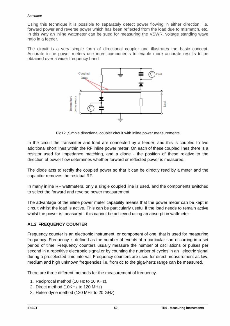
Annexure
IRISET 59 TB6 - Measuring instruments
Using this technique it is possible to separately detect power flowing in either direction, i.e. forward power and reverse power which has been reflected from the load due to mismatch, etc. In this way an inline wattmeter can be sued for measuring the VSWR, voltage standing wave ratio in a feeder. The circuit is a very simple form of directional coupler and illustrates the basic concept. Accurate inline power meters use more components to enable more accurate results to be obtained over a wider frequency band
Fig12 ,Simple directional coupler circuit with inline power measurements
In the circuit the transmitter and load are connected by a feeder, and this is coupled to two
additional short lines within the RF inline power meter. On each of these coupled lines there is a
resistor used for impedance matching, and a diode - the position of these relative to the
direction of power flow determines whether forward or reflected power is measured.
The diode acts to rectify the coupled power so that it can be directly read by a meter and the
capacitor removes the residual RF.
In many inline RF wattmeters, only a single coupled line is used, and the components switched
to select the forward and reverse power measurement.
The advantage of the inline power meter capability means that the power meter can be kept in
circuit whilst the load is active. This can be particularly useful if the load needs to remain active
whilst the power is measured - this cannot be achieved using an absorption wattmeter
A1.2 FREQUENCY COUNTER Frequency counter is an electronic instrument, or component of one, that is used for measuring
frequency. Frequency is defined as the number of events of a particular sort occurring in a set
period of time. Frequency counters usually measure the number of oscillations or pulses per
second in a repetitive electronic signal or by counting the number of cycles in an electric signal
during a preselected time interval. Frequency counters are used for direct measurement as low,
medium and high unknown frequencies i.e. from dc to the giga-hertz range can be measured.
There are three different methods for the measurement of frequency.
1. Reciprocal method (10 Hz to 10 KHz).
2. Direct method (10KHz to 120 MHz)
3. Heterodyne method (120 MHz to 20 GHz)
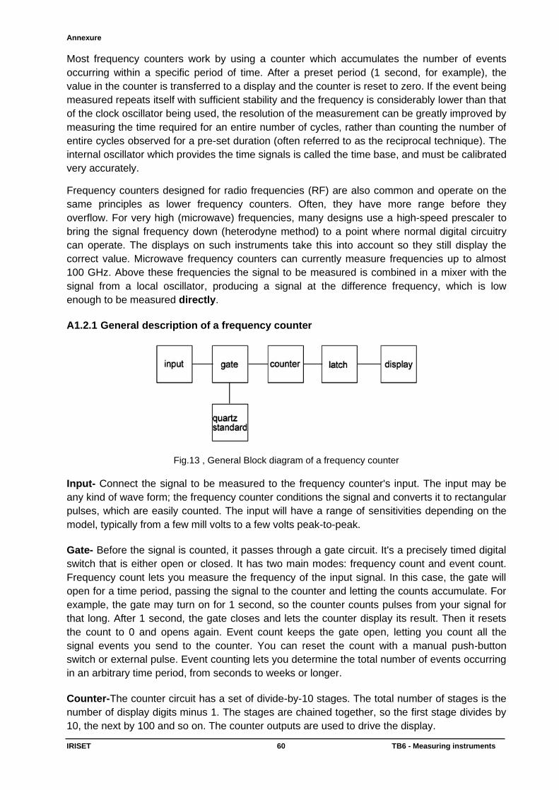
Annexure
IRISET 60 TB6 - Measuring instruments
Most frequency counters work by using a counter which accumulates the number of events
occurring within a specific period of time. After a preset period (1 second, for example), the
value in the counter is transferred to a display and the counter is reset to zero. If the event being
measured repeats itself with sufficient stability and the frequency is considerably lower than that
of the clock oscillator being used, the resolution of the measurement can be greatly improved by
measuring the time required for an entire number of cycles, rather than counting the number of
entire cycles observed for a pre-set duration (often referred to as the reciprocal technique). The
internal oscillator which provides the time signals is called the time base, and must be calibrated
very accurately.
Frequency counters designed for radio frequencies (RF) are also common and operate on the
same principles as lower frequency counters. Often, they have more range before they
overflow. For very high (microwave) frequencies, many designs use a high-speed prescaler to
bring the signal frequency down (heterodyne method) to a point where normal digital circuitry
can operate. The displays on such instruments take this into account so they still display the
correct value. Microwave frequency counters can currently measure frequencies up to almost
100 GHz. Above these frequencies the signal to be measured is combined in a mixer with the
signal from a local oscillator, producing a signal at the difference frequency, which is low
enough to be measured directly.
A1.2.1 General description of a frequency counter
Fig.13 , General Block diagram of a frequency counter
Input- Connect the signal to be measured to the frequency counter's input. The input may be
any kind of wave form; the frequency counter conditions the signal and converts it to rectangular
pulses, which are easily counted. The input will have a range of sensitivities depending on the
model, typically from a few mill volts to a few volts peak-to-peak.
Gate- Before the signal is counted, it passes through a gate circuit. It's a precisely timed digital
switch that is either open or closed. It has two main modes: frequency count and event count.
Frequency count lets you measure the frequency of the input signal. In this case, the gate will
open for a time period, passing the signal to the counter and letting the counts accumulate. For
example, the gate may turn on for 1 second, so the counter counts pulses from your signal for
that long. After 1 second, the gate closes and lets the counter display its result. Then it resets
the count to 0 and opens again. Event count keeps the gate open, letting you count all the
signal events you send to the counter. You can reset the count with a manual push-button
switch or external pulse. Event counting lets you determine the total number of events occurring
in an arbitrary time period, from seconds to weeks or longer.
Counter-The counter circuit has a set of divide-by-10 stages. The total number of stages is the
number of display digits minus 1. The stages are chained together, so the first stage divides by
10, the next by 100 and so on. The counter outputs are used to drive the display.
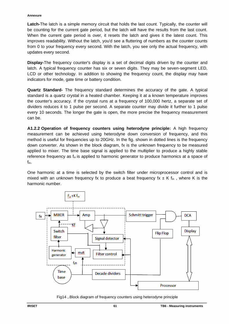
Annexure
IRISET 61 TB6 - Measuring instruments
Latch-The latch is a simple memory circuit that holds the last count. Typically, the counter will
be counting for the current gate period, but the latch will have the results from the last count.
When the current gate period is over, it resets the latch and gives it the latest count. This
improves readability. Without the latch, you'd see a fluttering of numbers as the counter counts
from 0 to your frequency every second. With the latch, you see only the actual frequency, with
updates every second.
Display-The frequency counter's display is a set of decimal digits driven by the counter and
latch. A typical frequency counter has six or seven digits. They may be seven-segment LED,
LCD or other technology. In addition to showing the frequency count, the display may have
indicators for mode, gate time or battery condition.
Quartz Standard- The frequency standard determines the accuracy of the gate. A typical
standard is a quartz crystal in a heated chamber. Keeping it at a known temperature improves
the counter's accuracy. If the crystal runs at a frequency of 100,000 hertz, a separate set of
dividers reduces it to 1 pulse per second. A separate counter may divide it further to 1 pulse
every 10 seconds. The longer the gate is open, the more precise the frequency measurement
can be.
A1.2.2 Operation of frequency counters using heterodyne principle: A high frequency
measurement can be achieved using heterodyne down conversion of frequency, and this
method is useful for frequencies up to 20GHz. In the fig. shown in dotted lines is the frequency
down converter. As shown in the block diagram, fx is the unknown frequency to be measured
applied to mixer. The time base signal is applied to the multiplier to produce a highly stable
reference frequency as fin is applied to harmonic generator to produce harmonics at a space of
fin.
One harmonic at a time is selected by the switch filter under microprocessor control and is
mixed with an unknown frequency fx to produce a beat frequency fx ± K fin , where K is the
harmonic number.
Fig14 ,.Block diagram of frequency counters using heterodyne principle
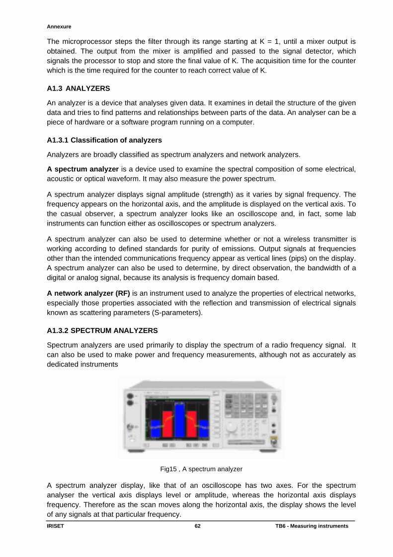
Annexure
IRISET 62 TB6 - Measuring instruments
The microprocessor steps the filter through its range starting at K = 1, until a mixer output is
obtained. The output from the mixer is amplified and passed to the signal detector, which
signals the processor to stop and store the final value of K. The acquisition time for the counter
which is the time required for the counter to reach correct value of K.
A1.3 ANALYZERS
An analyzer is a device that analyses given data. It examines in detail the structure of the given
data and tries to find patterns and relationships between parts of the data. An analyser can be a
piece of hardware or a software program running on a computer.
A1.3.1 Classification of analyzers
Analyzers are broadly classified as spectrum analyzers and network analyzers.
A spectrum analyzer is a device used to examine the spectral composition of some electrical,
acoustic or optical waveform. It may also measure the power spectrum.
A spectrum analyzer displays signal amplitude (strength) as it varies by signal frequency. The
frequency appears on the horizontal axis, and the amplitude is displayed on the vertical axis. To
the casual observer, a spectrum analyzer looks like an oscilloscope and, in fact, some lab
instruments can function either as oscilloscopes or spectrum analyzers.
A spectrum analyzer can also be used to determine whether or not a wireless transmitter is
working according to defined standards for purity of emissions. Output signals at frequencies
other than the intended communications frequency appear as vertical lines (pips) on the display.
A spectrum analyzer can also be used to determine, by direct observation, the bandwidth of a
digital or analog signal, because its analysis is frequency domain based.
A network analyzer (RF) is an instrument used to analyze the properties of electrical networks,
especially those properties associated with the reflection and transmission of electrical signals
known as scattering parameters (S-parameters).
A1.3.2 SPECTRUM ANALYZERS
Spectrum analyzers are used primarily to display the spectrum of a radio frequency signal. It
can also be used to make power and frequency measurements, although not as accurately as
dedicated instruments
Fig15 , A spectrum analyzer
A spectrum analyzer display, like that of an oscilloscope has two axes. For the spectrum
analyser the vertical axis displays level or amplitude, whereas the horizontal axis displays
frequency. Therefore as the scan moves along the horizontal axis, the display shows the level
of any signals at that particular frequency.

Annexure
IRISET 63 TB6 - Measuring instruments
This means that the spectrum analyser, as the name indicates analyses the spectrum of a
signal. It shows the relative levels of signals on different frequencies within the range of the
particular sweep or scan. In view of the very large variations in signal level that are expected.
These are calibrated in dB in line with many other measurements that made for signal
amplitudes. The horizontal scale conversely is normally linear. This can be adjusted to cover the
required range. The term span is used to give the complete calibrated range across the screen.
Fig 16 General format of the display on a spectrum analyzer
A1.3.2.1 Types of spectrum analyser Just as in the case of other instruments, there are a number of types of spectrum analyzer that
can be seen in the manufacturers catalogues.
• Swept or super heterodyne spectrum analysers: The operation of the swept frequency
spectrum analyzer is based on the use of the super heterodyne principle, sweeping the
frequency that is analysed across the required band to produce a view of the signals with
their relative strengths. This may be considered as the more traditional form of spectrum
analyser, and it is the type that is most widely used.
• Fast Fourier Transform, FFT analysers: These spectrum analyzers use a form of
Fourier transform known as a Fast Fourier Transform (FFT) converting the signals into a
digital format for analysis digitally. These analysers are more expensive and often more
specialised.
A1.3.2.1a Swept or super heterodyne spectrum analyser Super heterodyne spectrum analyzer technology also referred to as sweep or swept frequency
spectrum analyzer technology is widely used within analyzers to make RF measurements.
Super heterodyne or sweep analyzers offer very high levels of performance, especially when
compared to what was available a few years ago. Typically today they make widespread use of
digital signal processing techniques, the signals being converted into a digital format after the IF
stage. This enables very flexible filtering to be offered along with a host of other useful facilities
that would not be possible if only analogue techniques were employed
The swept spectrum analyser uses the same super heterodyne principle used in many radio
receivers as the underlying principle on which its operation depends. The super heterodyne
principle uses a mixer and a second, locally generated local oscillator signal to translate the
frequency.
Frequency
Signals
Noise
Am
plitu
de
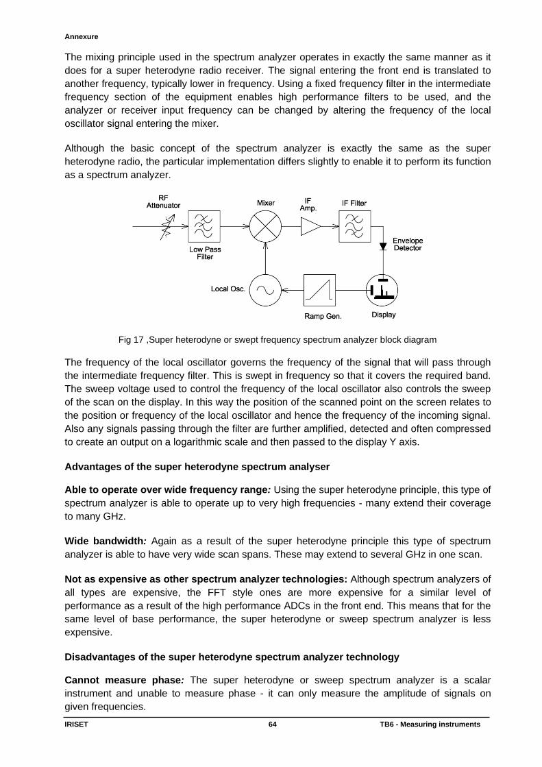
Annexure
IRISET 64 TB6 - Measuring instruments
The mixing principle used in the spectrum analyzer operates in exactly the same manner as it
does for a super heterodyne radio receiver. The signal entering the front end is translated to
another frequency, typically lower in frequency. Using a fixed frequency filter in the intermediate
frequency section of the equipment enables high performance filters to be used, and the
analyzer or receiver input frequency can be changed by altering the frequency of the local
oscillator signal entering the mixer.
Although the basic concept of the spectrum analyzer is exactly the same as the super
heterodyne radio, the particular implementation differs slightly to enable it to perform its function
as a spectrum analyzer.
Fig 17 ,Super heterodyne or swept frequency spectrum analyzer block diagram
The frequency of the local oscillator governs the frequency of the signal that will pass through
the intermediate frequency filter. This is swept in frequency so that it covers the required band.
The sweep voltage used to control the frequency of the local oscillator also controls the sweep
of the scan on the display. In this way the position of the scanned point on the screen relates to
the position or frequency of the local oscillator and hence the frequency of the incoming signal.
Also any signals passing through the filter are further amplified, detected and often compressed
to create an output on a logarithmic scale and then passed to the display Y axis.
Advantages of the super heterodyne spectrum analyser Able to operate over wide frequency range: Using the super heterodyne principle, this type of
spectrum analyzer is able to operate up to very high frequencies - many extend their coverage
to many GHz.
Wide bandwidth: Again as a result of the super heterodyne principle this type of spectrum
analyzer is able to have very wide scan spans. These may extend to several GHz in one scan.
Not as expensive as other spectrum analyzer technologies: Although spectrum analyzers of
all types are expensive, the FFT style ones are more expensive for a similar level of
performance as a result of the high performance ADCs in the front end. This means that for the
same level of base performance, the super heterodyne or sweep spectrum analyzer is less
expensive.
Disadvantages of the super heterodyne spectrum analyzer technology Cannot measure phase: The super heterodyne or sweep spectrum analyzer is a scalar
instrument and unable to measure phase - it can only measure the amplitude of signals on
given frequencies.
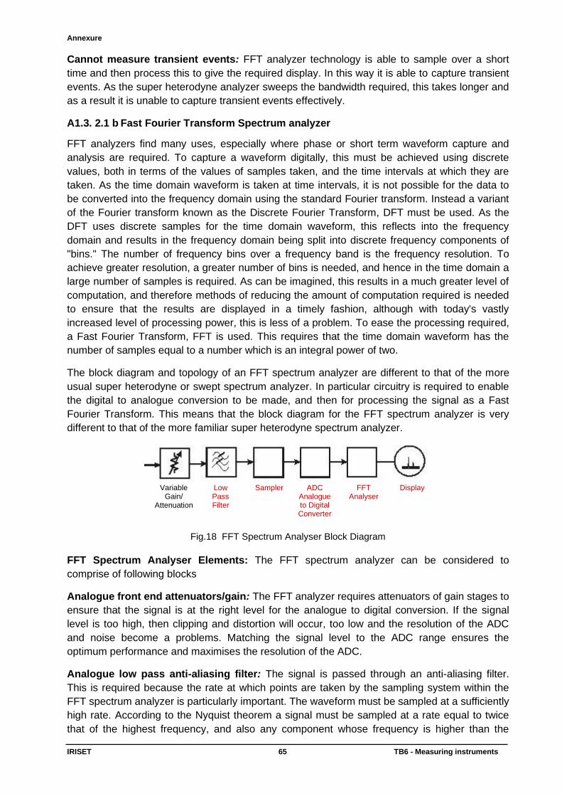
Annexure
IRISET 65 TB6 - Measuring instruments
Cannot measure transient events: FFT analyzer technology is able to sample over a short
time and then process this to give the required display. In this way it is able to capture transient
events. As the super heterodyne analyzer sweeps the bandwidth required, this takes longer and
as a result it is unable to capture transient events effectively.
A1.3. 2.1 b Fast Fourier Transform Spectrum analyzer
FFT analyzers find many uses, especially where phase or short term waveform capture and
analysis are required. To capture a waveform digitally, this must be achieved using discrete
values, both in terms of the values of samples taken, and the time intervals at which they are
taken. As the time domain waveform is taken at time intervals, it is not possible for the data to
be converted into the frequency domain using the standard Fourier transform. Instead a variant
of the Fourier transform known as the Discrete Fourier Transform, DFT must be used. As the
DFT uses discrete samples for the time domain waveform, this reflects into the frequency
domain and results in the frequency domain being split into discrete frequency components of
"bins." The number of frequency bins over a frequency band is the frequency resolution. To
achieve greater resolution, a greater number of bins is needed, and hence in the time domain a
large number of samples is required. As can be imagined, this results in a much greater level of
computation, and therefore methods of reducing the amount of computation required is needed
to ensure that the results are displayed in a timely fashion, although with today's vastly
increased level of processing power, this is less of a problem. To ease the processing required,
a Fast Fourier Transform, FFT is used. This requires that the time domain waveform has the
number of samples equal to a number which is an integral power of two.
The block diagram and topology of an FFT spectrum analyzer are different to that of the more
usual super heterodyne or swept spectrum analyzer. In particular circuitry is required to enable
the digital to analogue conversion to be made, and then for processing the signal as a Fast
Fourier Transform. This means that the block diagram for the FFT spectrum analyzer is very
different to that of the more familiar super heterodyne spectrum analyzer.
Fig.18 FFT Spectrum Analyser Block Diagram
FFT Spectrum Analyser Elements: The FFT spectrum analyzer can be considered to
comprise of following blocks
Analogue front end attenuators/gain: The FFT analyzer requires attenuators of gain stages to
ensure that the signal is at the right level for the analogue to digital conversion. If the signal
level is too high, then clipping and distortion will occur, too low and the resolution of the ADC
and noise become a problems. Matching the signal level to the ADC range ensures the
optimum performance and maximises the resolution of the ADC.
Analogue low pass anti-aliasing filter: The signal is passed through an anti-aliasing filter.
This is required because the rate at which points are taken by the sampling system within the
FFT spectrum analyzer is particularly important. The waveform must be sampled at a sufficiently
high rate. According to the Nyquist theorem a signal must be sampled at a rate equal to twice
that of the highest frequency, and also any component whose frequency is higher than the
Variable Gain/
Attenuation
Low Pass Filter
Sampler ADC Analogue to Digital Converter
FFT Analyser
Display

Annexure
IRISET 66 TB6 - Measuring instruments
Nyquist rate will appear in the measurement as a lower frequency component - a factor known
as "aliasing". This results from, where the actual values of the higher rate fall when the samples
are taken. To avoid aliasing a low pass filter is placed ahead of the sampler to remove any
unwanted high frequency elements. This filter must have a cut-off frequency which is less than
half the sampling rate, although typically to provide some margin, the low pass filter cut-off
frequency is at highest 2.5 times less than the sampling rate of the FFT spectrum analyzer. In
turn this determines the maximum frequency of operation of the FFT spectrum analyzer.
Sampling and analogue to digital conversion: In order to perform the analogue to digital
conversion, two elements are required. The first is a sampler which takes samples at discrete
time intervals - the sampling rate. The importance of this rate has been discussed above. The
samples are then passed to an analogue to digital converter which produces the digital format
for the samples that is required for the FFT analysis.
FFT analyzer: With the data from the sampler, which is in the time domain, this is then
converted into the frequency domain by the FFT analyzer. This is then able to further process
the data using digital signal processing techniques to analyze the data in the format required.
Display: With the power of processing it is possible to present the information for display in a
variety of ways. Today's displays are very flexible and enable the information to be presented in
formats that are easy to comprehend and reveal a variety of facets of the signal. The display
elements of the FFT spectrum analyzer are therefore very important so that the information
captured and processed can be suitably presented for the user.
Advantages of FFT spectrum analyzer technology
Fast capture of waveform: In view of the fact that the waveform is analysed digitally, the
waveform can be captured in a relatively short time, and subsequently analysed. This short
capture time can have many advantages.
Able to capture non-repetitive events: The short capture time means that the FFT analyzer
can capture non-repetitive waveforms, giving them a capability not possible with other spectrum
analyzers.
Able to analyse signal phase: As part of the signal capture process, data is gained which can
be processed to reveal the phase of signals.
Disadvantages of the FFT spectrum analyzer technology
Frequency limitations: The main limit of the frequency and bandwidth of FFT spectrum
analyzers is the analogue to digital converter, ADC that is used to convert the analogue signal
into a digital format. While technology is improving this component still places a major limitation
on the upper frequency limits or the bandwidth if a down-conversion stage is used.
Cost: The high level of performance required by the ADC means that this item is a very high
cost item. In addition to all the other processing and display circuitry required, this results in the
costs rising for these items.
A1.3. 3 Network analyser: Network analyzers are used mostly at high frequencies; operating in
the range 9 kHz to 110 GHz. Special types of network analyzers can also cover lower frequency
ranges down to 1 Hz. These network analyzers can be used for example for the stability
analysis of open loops or for the measurement of audio and ultrasonic components. RF network
analyser is used to measure the properties of RF devices.
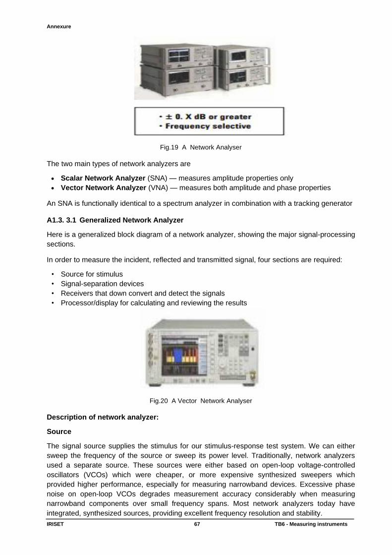
Annexure
IRISET 67 TB6 - Measuring instruments
Fig.19 A Network Analyser
The two main types of network analyzers are
• Scalar Network Analyzer (SNA) — measures amplitude properties only
• Vector Network Analyzer (VNA) — measures both amplitude and phase properties
An SNA is functionally identical to a spectrum analyzer in combination with a tracking generator A1.3. 3.1 Generalized Network Analyzer
Here is a generalized block diagram of a network analyzer, showing the major signal-processing
sections.
In order to measure the incident, reflected and transmitted signal, four sections are required:
• Source for stimulus
• Signal-separation devices
• Receivers that down convert and detect the signals
• Processor/display for calculating and reviewing the results
Fig.20 A Vector Network Analyser
Description of network analyzer:
Source
The signal source supplies the stimulus for our stimulus-response test system. We can either
sweep the frequency of the source or sweep its power level. Traditionally, network analyzers
used a separate source. These sources were either based on open-loop voltage-controlled
oscillators (VCOs) which were cheaper, or more expensive synthesized sweepers which
provided higher performance, especially for measuring narrowband devices. Excessive phase
noise on open-loop VCOs degrades measurement accuracy considerably when measuring
narrowband components over small frequency spans. Most network analyzers today have
integrated, synthesized sources, providing excellent frequency resolution and stability.
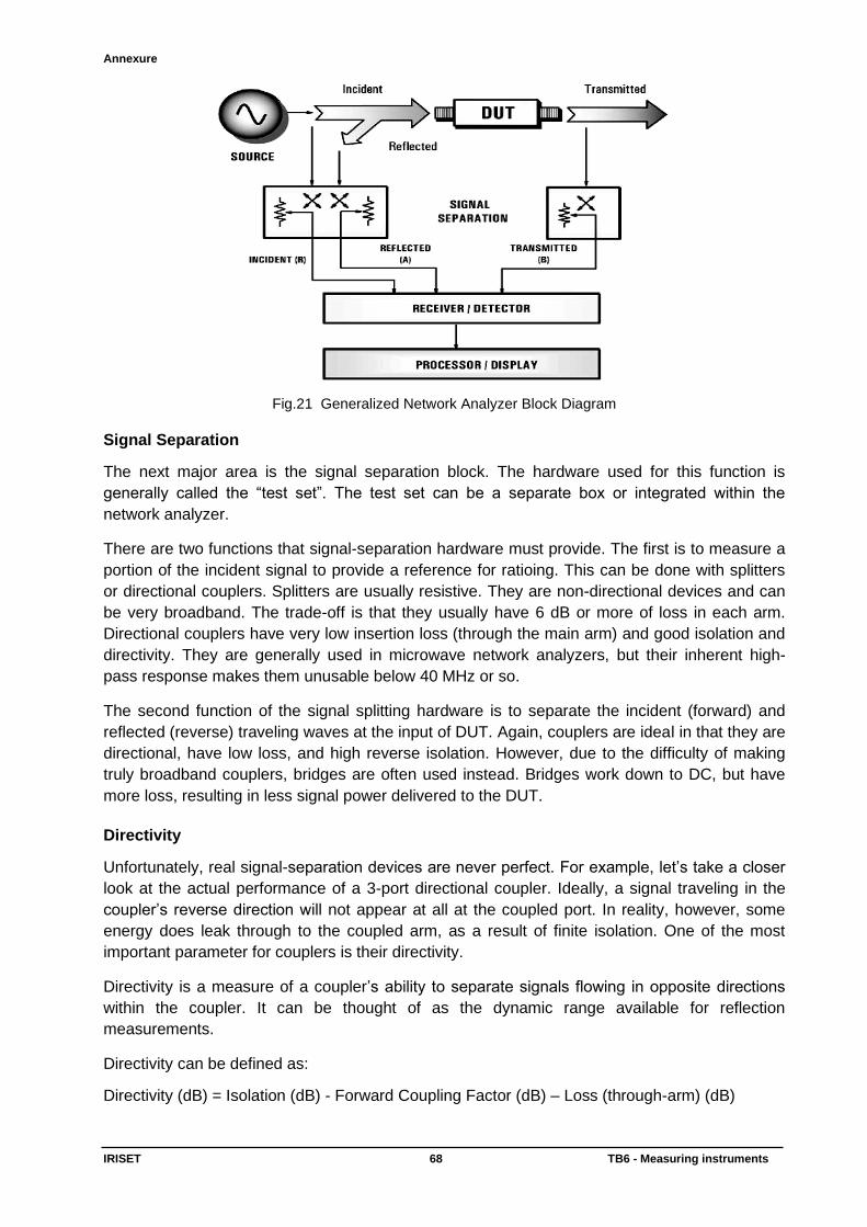
Annexure
IRISET 68 TB6 - Measuring instruments
Fig.21 Generalized Network Analyzer Block Diagram
Signal Separation
The next major area is the signal separation block. The hardware used for this function is
generally called the “test set”. The test set can be a separate box or integrated within the
network analyzer.
There are two functions that signal-separation hardware must provide. The first is to measure a
portion of the incident signal to provide a reference for ratioing. This can be done with splitters
or directional couplers. Splitters are usually resistive. They are non-directional devices and can
be very broadband. The trade-off is that they usually have 6 dB or more of loss in each arm.
Directional couplers have very low insertion loss (through the main arm) and good isolation and
directivity. They are generally used in microwave network analyzers, but their inherent high-
pass response makes them unusable below 40 MHz or so.
The second function of the signal splitting hardware is to separate the incident (forward) and
reflected (reverse) traveling waves at the input of DUT. Again, couplers are ideal in that they are
directional, have low loss, and high reverse isolation. However, due to the difficulty of making
truly broadband couplers, bridges are often used instead. Bridges work down to DC, but have
more loss, resulting in less signal power delivered to the DUT.
Directivity
Unfortunately, real signal-separation devices are never perfect. For example, let’s take a closer
look at the actual performance of a 3-port directional coupler. Ideally, a signal traveling in the
coupler’s reverse direction will not appear at all at the coupled port. In reality, however, some
energy does leak through to the coupled arm, as a result of finite isolation. One of the most
important parameter for couplers is their directivity.
Directivity is a measure of a coupler’s ability to separate signals flowing in opposite directions
within the coupler. It can be thought of as the dynamic range available for reflection
measurements.
Directivity can be defined as:
Directivity (dB) = Isolation (dB) - Forward Coupling Factor (dB) – Loss (through-arm) (dB)
Annexure
IRISET 69 TB6 - Measuring instruments
Detector Types The next portion of the network analyzer is the signal detection block. There are two basic ways
of providing signal detection in network analyzers. Diode detectors convert the RF signal level to
a proportional DC level. If the stimulus signal is amplitude modulated, the diode strips the RF
carrier from the modulation (this is called AC detection). Diode detection is inherently scalar, as
phase information of the RF carrier is lost. The tuned receiver uses a local oscillator (LO) to mix
the RF down to a lower “intermediate” frequency (IF). The LO is either locked to the RF or the IF
signal so that the receivers in the network analyzer are always tuned to the RF signal present at
the input. The IF signal is band pass filtered, which narrows the receiver bandwidth and greatly
improves sensitivity and dynamic range. Modern analyzers use an analog-to-digital converter
(ADC) and digital-signal processing (DSP) to extract magnitude and phase information from the
IF signal. The tuned-receiver approach is used in vector network analyzers and spectrum
analyzers.
Processor/Display The last major block of hardware in the network analyzer is the display/processor section. This
is where the reflection and transmission data is formatted in ways that make it easy to interpret
the measurement results. Most network analyzers have similar features such as linear and
logarithmic sweeps, linear and log formats, polar plots, Smith charts, etc. Other common
features are trace markers, limit lines and pass/fail testing.
A1.3.3.2 What is the Difference between Network and Spectrum Analyzers? Now that we have seen some of the measurements that are commonly done with network and
spectrum analyzers, it might be helpful to review the main differences between these
instruments. Although they often both contain tuned receivers operating over similar frequency
ranges, they are optimized for very different measurement applications. Network analyzers are
used to measure components, devices, circuits and sub-assemblies. They contain both a
source and multiple receivers, and generally display ratioed amplitude and phase information
(frequency or power sweeps). A network analyzer is always looking at a known signal (in terms
of frequency), since it is a stimulus response system. With network analyzers, it is harder to get
an accurate trace on the display, but very easy to interpret the results. With vector-error
correction, network analyzers provide much higher measurement accuracy than spectrum
analyzers. Spectrum analyzers are most often used to measure signal characteristics such as
carrier level, sidebands, harmonics, phase noise etc. on unknown signals. They are most
commonly configured as a single channel receiver, without a source. Because of the flexibility
needed to analyze signals, spectrum analyzers generally have a much wider range of IF
bandwidths available than most network analyzers. Spectrum analyzers are often used with
external sources for nonlinear stimulus/response testing. When combined with a tracking
generator, spectrum analyzers can be used for scalar component testing (magnitude versus
frequency, but no phase measurements). With spectrum analyzers, it is easy to get a trace on
the display, but interpreting the results can be much more difficult than with a network analyzer.
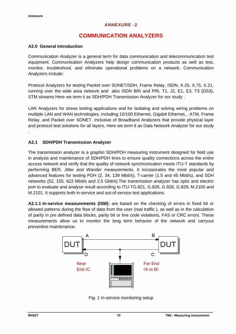
Annexure
IRISET 70 TB6 - Measuring instruments
ANNEXURE -2
COMMUNICATION ANALYZERS A2.0 General Introduction Communication Analyzer is a general term for data communication and telecommunication test
equipment. Communication Analyzers help design communication products as well as test,
monitor, troubleshoot, and eliminate operational problems on a network. Communication
Analyzers include:
Protocol Analyzers for testing Packet over SONET/SDH, Frame Relay, ISDN, X.25, X.75, X.21,
running over the wide area network and also ISDN BRI and PRI, T1, J2, E1, E3, T3 (DS3),
STM streams Here we term it as SDH/PDH Transmission Analyzer for our study .
LAN Analyzers for stress testing applications and for isolating and solving wiring problems on
multiple LAN and WAN technologies, including 10/100 Ethernet, Gigabit Ethernet, , ATM, Frame
Relay, and Packet over SONET. Inclusive of Broadband Analyzers that provide physical layer
and protocol test solutions for all layers, Here we term it as Data Network Analyzer for our study
.
A2.1 SDH/PDH Transmission Analyzer The transmission analyzer is a graphic SDH/PDH measuring instrument designed for field use
in analysis and maintenance of SDH/PDH lines to ensure quality connections across the entire
access network and verify that the quality of network synchronization meets ITU-T standards by
performing BER, Jitter and Wander measurements. It incorporates the most popular and
advanced features for testing PDH (2, 34, 139 Mbit/s), T-carrier (1.5 and 45 Mbit/s), and SDH
networks (52, 155, 622 Mbit/s and 2.5 Gbit/s).The transmission analyzer has optic and electric
port to evaluate and analyse result according to ITU-TG.821, G.826, G.828, G.829, M.2100 and
M.2101. It supports both in-service and out-of-service test applications.
A2.1.1 In-service measurements (ISM): are based on the checking of errors in fixed bit or
allowed patterns during the flow of data from the user (real traffic ), as well as in the calculation
of parity in pre defined data blocks, parity bit or line code violations, FAS or CRC errors. These
measurements allow us to monitor the long term behavior of the network and carryout
preventive maintenance.
Fig. 1 In-service monitoring setup
Near
End (C
to D)
Far End
(A to B)
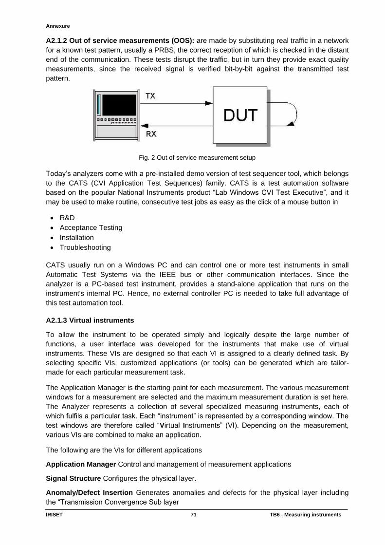
Annexure
IRISET 71 TB6 - Measuring instruments
A2.1.2 Out of service measurements (OOS): are made by substituting real traffic in a network
for a known test pattern, usually a PRBS, the correct reception of which is checked in the distant
end of the communication. These tests disrupt the traffic, but in turn they provide exact quality
measurements, since the received signal is verified bit-by-bit against the transmitted test
pattern.
Fig. 2 Out of service measurement setup
Today’s analyzers come with a pre-installed demo version of test sequencer tool, which belongs
to the CATS (CVI Application Test Sequences) family. CATS is a test automation software
based on the popular National Instruments product “Lab Windows CVI Test Executive”, and it
may be used to make routine, consecutive test jobs as easy as the click of a mouse button in
• R&D
• Acceptance Testing
• Installation
• Troubleshooting
CATS usually run on a Windows PC and can control one or more test instruments in small
Automatic Test Systems via the IEEE bus or other communication interfaces. Since the
analyzer is a PC-based test instrument, provides a stand-alone application that runs on the
instrument's internal PC. Hence, no external controller PC is needed to take full advantage of
this test automation tool.
A2.1.3 Virtual instruments
To allow the instrument to be operated simply and logically despite the large number of
functions, a user interface was developed for the instruments that make use of virtual
instruments. These VIs are designed so that each VI is assigned to a clearly defined task. By
selecting specific VIs, customized applications (or tools) can be generated which are tailor-
made for each particular measurement task.
The Application Manager is the starting point for each measurement. The various measurement
windows for a measurement are selected and the maximum measurement duration is set here.
The Analyzer represents a collection of several specialized measuring instruments, each of
which fulfils a particular task. Each “instrument” is represented by a corresponding window. The
test windows are therefore called “Virtual Instruments” (VI). Depending on the measurement,
various VIs are combined to make an application.
The following are the VIs for different applications
Application Manager Control and management of measurement applications
Signal Structure Configures the physical layer.
Anomaly/Defect Insertion Generates anomalies and defects for the physical layer including
the “Transmission Convergence Sub layer
Annexure
IRISET 72 TB6 - Measuring instruments
Anomaly/Defect Analyzer Analyzes anomalies and defects for the physical layer including the
“Transmission Convergence Sub layer”.
Overhead Generator Edit physical frame overhead information. Used with SDH, SONET and
PDH/ATM frames to G.832 (34 Mbit/s and 140 Mbit/s).
Overhead Analyzer Analyzes physical frame overhead information. Used with SDH, SONET
and PDH/ATM frames to G.832 (34 Mbit/s and 140 Mbit/s).
Pointer Generator / Analyzer Generates and Analyzes SDH/SONET pointers.
PDH Generator/Analyzer Set and display physical frame overhead. Used with PDH frames.
Performance Analysis Performance analysis to G.821, G.826, M.2100, M.2101 and Bell
core/ANSI.
These VIs have overall control of
· Measurement applications
· Measurement results generated using the applications
· Measurement sequence.
A2.1.4 Performance Analysis by using SDH/PDH Transmission Analyzer:
Performance Analysis: These measurements are performed in order to determine the quality
of a transmission path. The measurements are based on the corresponding ITU-T
Recommendations of G.821, G.826, G.828, G.829, M.2100 and M.2101.
ITU-T G.826 evaluation: The G.826 analysis is separated into ISM (in-service measurement)
and OOS (out of service measurement). OOS is mainly used for aligning newly set-up
communications equipment. Unframed test signals are measured and block errors are
evaluated. ISM, as the name implies, allows measurement while the system is operational.
This Recommendation defines error performance parameters and objectives for international
digital paths which operate at or above the primary rate. The objectives given are independent
of the physical network supporting the path. These paths may be based on a Plesiochronous
Digital Hierarchy, Synchronous Digital Hierarchy or some other transport network such as cell-
based This Recommendation is based upon a block-based measurement concept using error
detection codes inherent to the path under test.
Anomalies: In-service anomaly conditions are used to determine the error performance of a
PDH path when the path is not in a defect state. The two following categories of anomalies
related to the incoming signal are defined:
a1 an errored frame alignment signal;
a2 an EB as indicated by an EDC
Defects: In-service defect conditions are used in the G.730 to G.750 series of
Recommendations relevant to PDH multiplex equipment to determine the change of
performance state which may occur on a path.
The three following categories of defects related to the incoming signal are defined:
d1 loss of signal;
d2 alarm indication signal;
d3 loss of frame alignment.
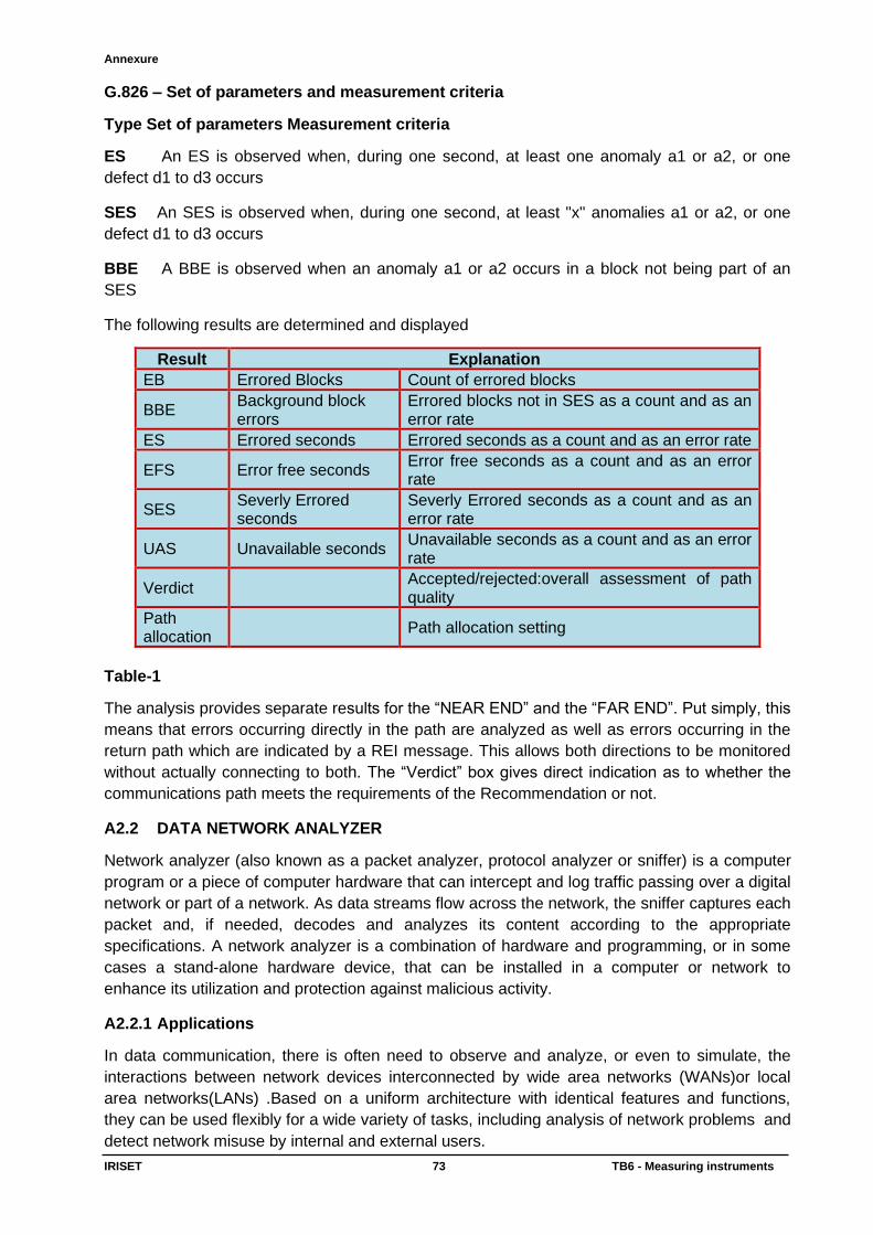
Annexure
IRISET 73 TB6 - Measuring instruments
G.826 – Set of parameters and measurement criteria
Type Set of parameters Measurement criteria
ES An ES is observed when, during one second, at least one anomaly a1 or a2, or one
defect d1 to d3 occurs
SES An SES is observed when, during one second, at least "x" anomalies a1 or a2, or one
defect d1 to d3 occurs
BBE A BBE is observed when an anomaly a1 or a2 occurs in a block not being part of an
SES
The following results are determined and displayed
Result Explanation
EB Errored Blocks Count of errored blocks
BBE Background block errors
Errored blocks not in SES as a count and as an error rate
ES Errored seconds Errored seconds as a count and as an error rate
EFS Error free seconds Error free seconds as a count and as an error rate
SES Severly Errored seconds
Severly Errored seconds as a count and as an error rate
UAS Unavailable seconds Unavailable seconds as a count and as an error rate
Verdict Accepted/rejected:overall assessment of path quality
Path allocation
Path allocation setting
Table-1
The analysis provides separate results for the “NEAR END” and the “FAR END”. Put simply, this
means that errors occurring directly in the path are analyzed as well as errors occurring in the
return path which are indicated by a REI message. This allows both directions to be monitored
without actually connecting to both. The “Verdict” box gives direct indication as to whether the
communications path meets the requirements of the Recommendation or not.
A2.2 DATA NETWORK ANALYZER
Network analyzer (also known as a packet analyzer, protocol analyzer or sniffer) is a computer
program or a piece of computer hardware that can intercept and log traffic passing over a digital
network or part of a network. As data streams flow across the network, the sniffer captures each
packet and, if needed, decodes and analyzes its content according to the appropriate
specifications. A network analyzer is a combination of hardware and programming, or in some
cases a stand-alone hardware device, that can be installed in a computer or network to
enhance its utilization and protection against malicious activity.
A2.2.1 Applications
In data communication, there is often need to observe and analyze, or even to simulate, the
interactions between network devices interconnected by wide area networks (WANs)or local
area networks(LANs) .Based on a uniform architecture with identical features and functions,
they can be used flexibly for a wide variety of tasks, including analysis of network problems and
detect network misuse by internal and external users.
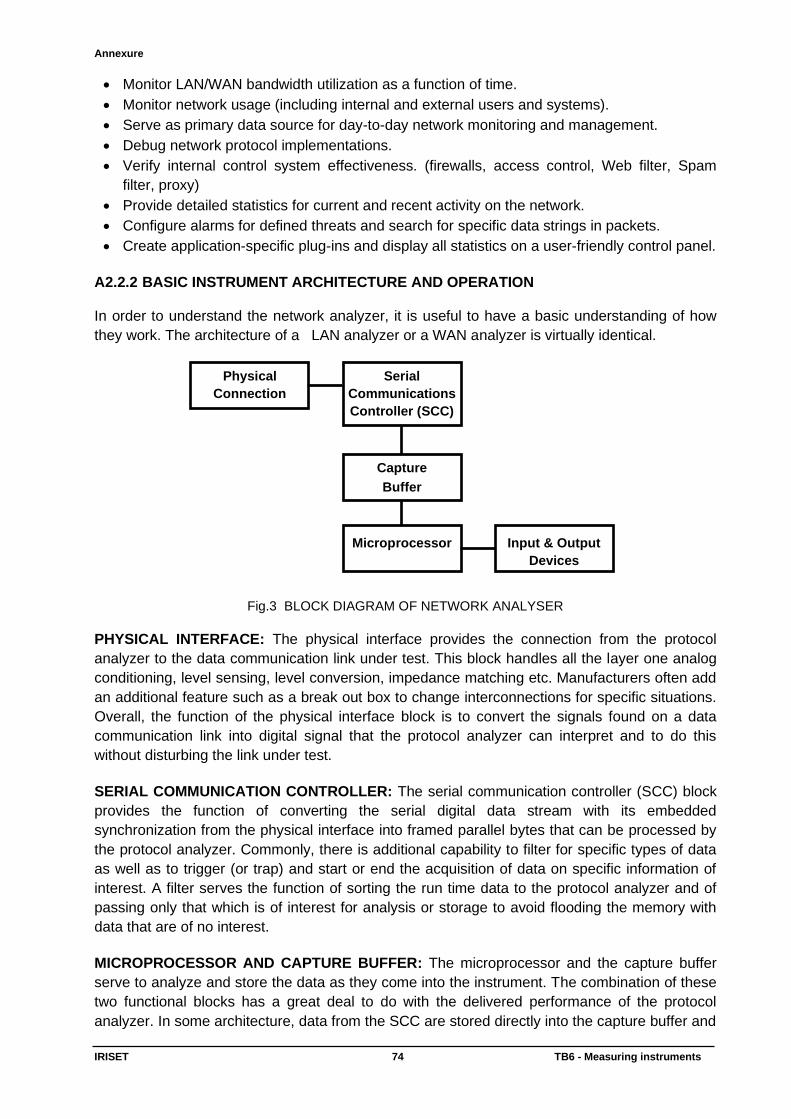
Annexure
IRISET 74 TB6 - Measuring instruments
• Monitor LAN/WAN bandwidth utilization as a function of time.
• Monitor network usage (including internal and external users and systems).
• Serve as primary data source for day-to-day network monitoring and management.
• Debug network protocol implementations.
• Verify internal control system effectiveness. (firewalls, access control, Web filter, Spam
filter, proxy)
• Provide detailed statistics for current and recent activity on the network.
• Configure alarms for defined threats and search for specific data strings in packets.
• Create application-specific plug-ins and display all statistics on a user-friendly control panel.
A2.2.2 BASIC INSTRUMENT ARCHITECTURE AND OPERATION In order to understand the network analyzer, it is useful to have a basic understanding of how
they work. The architecture of a LAN analyzer or a WAN analyzer is virtually identical.
Fig.3 BLOCK DIAGRAM OF NETWORK ANALYSER
PHYSICAL INTERFACE: The physical interface provides the connection from the protocol
analyzer to the data communication link under test. This block handles all the layer one analog
conditioning, level sensing, level conversion, impedance matching etc. Manufacturers often add
an additional feature such as a break out box to change interconnections for specific situations.
Overall, the function of the physical interface block is to convert the signals found on a data
communication link into digital signal that the protocol analyzer can interpret and to do this
without disturbing the link under test.
SERIAL COMMUNICATION CONTROLLER: The serial communication controller (SCC) block
provides the function of converting the serial digital data stream with its embedded
synchronization from the physical interface into framed parallel bytes that can be processed by
the protocol analyzer. Commonly, there is additional capability to filter for specific types of data
as well as to trigger (or trap) and start or end the acquisition of data on specific information of
interest. A filter serves the function of sorting the run time data to the protocol analyzer and of
passing only that which is of interest for analysis or storage to avoid flooding the memory with
data that are of no interest.
MICROPROCESSOR AND CAPTURE BUFFER: The microprocessor and the capture buffer
serve to analyze and store the data as they come into the instrument. The combination of these
two functional blocks has a great deal to do with the delivered performance of the protocol
analyzer. In some architecture, data from the SCC are stored directly into the capture buffer and
Physical
Connection
Serial
Communications
Controller (SCC)
Microprocessor Input & Output
Devices
Capture
Buffer
Annexure
IRISET 75 TB6 - Measuring instruments
the processor then operates on the data to provide analysis. This method is appropriate for
applications where the user needs to acquire limited amounts of high-speed data and keep the
cost of the instrument’s hardware low. The architecture tends to consume memory very quickly,
resulting in a shallow effective capture size. On the other hand, if the processor first formats and
adds information to the data before storing it into the buffer memory, it could be overrun by the
speed of data.
INPUT AND OUTPUT DEVICE: The input and output block in the block diagram is simply the
display, keyboard and local mass storage for the instrument. Presentation through the user
interface is an important dimension for consideration. The tradeoff with this part of the
instrument is usually one of simplicity of operation versus the versatility and flexibility afforded
by it. Soft key assistance, use of graphic user interface and inclusion of a programming
language to control the instrument are common implementations each with its own special
value.
A2.2.3 SET UP On wired broadcast LANs, depending on the network structure (hub or switch), one can capture
traffic on all or just parts of the network from a single machine within the network; however,
there are some methods to avoid traffic narrowing by switches to gain access to traffic from
other systems on the network (e.g. ARP spoofing). For network monitoring purposes it may also
be desirable to monitor all data packets in a LAN by using a network switch with a so-called
monitoring port, whose purpose is to mirror all packets passing through all ports of the switch
when systems (computers) are connected to a switch port.
On wireless LANs, one can capture traffic on a particular channel. On wired broadcast and
wireless LANs, to capture traffic other than uni cast traffic sent to the machine running the
sniffer software, multicast traffic sent to a multicast group to which that machine is listening, and
broadcast traffic, the network adapter being used to capture the traffic must be put into
promiscuous mode; some sniffers support this, others don't. On wireless LANs, even if the
adapter is in promiscuous mode, packets not for the service set for which the adapter is
configured will usually be ignored. To see those packets, the adapter must be in monitor mode .
Promiscuous mode is a configuration of a network card that makes the card pass all traffic it
receives to the central processing unit rather than just frames addressed to it — a feature
normally used for packet sniffing, and bridged networking for hardware virtualization
The captured information is decoded from raw digital form into a human-readable format that
permits users of the protocol analyzer to easily review the exchanged information. Protocol
analyzers vary in their abilities to display data in multiple views, automatically detect errors,
determine the root causes of errors, generate timing diagrams etc.
Some protocol analyzers can also generate traffic and thus act as the reference device; these
can act as protocol testers. Such testers generate protocol-correct traffic for functional testing,
and may also have the ability to deliberately introduce errors to test for the DUT's ability to deal
with error conditions. Network analyzers are not intended to replace firewalls, anti-virus
programs, or spy ware detection programs. However, the use of a network analyzer in addition
to other countermeasures can minimize the probability that an attack will occur, and can
facilitate rapid response in the event an attack begins.
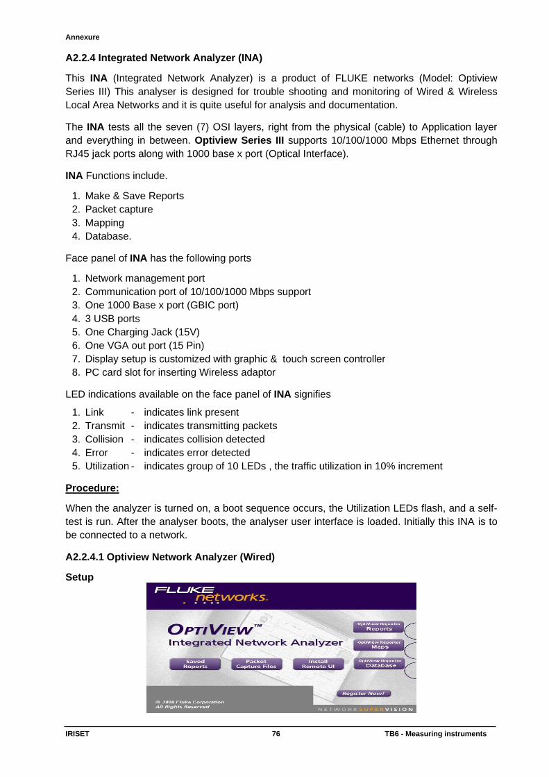
Annexure
IRISET 76 TB6 - Measuring instruments
A2.2.4 Integrated Network Analyzer (INA)
This INA (Integrated Network Analyzer) is a product of FLUKE networks (Model: Optiview
Series III) This analyser is designed for trouble shooting and monitoring of Wired & Wireless
Local Area Networks and it is quite useful for analysis and documentation.
The INA tests all the seven (7) OSI layers, right from the physical (cable) to Application layer
and everything in between. Optiview Series III supports 10/100/1000 Mbps Ethernet through
RJ45 jack ports along with 1000 base x port (Optical Interface).
INA Functions include.
1. Make & Save Reports
2. Packet capture
3. Mapping
4. Database.
Face panel of INA has the following ports
1. Network management port
2. Communication port of 10/100/1000 Mbps support
3. One 1000 Base x port (GBIC port)
4. 3 USB ports
5. One Charging Jack (15V)
6. One VGA out port (15 Pin)
7. Display setup is customized with graphic & touch screen controller
8. PC card slot for inserting Wireless adaptor
LED indications available on the face panel of INA signifies
1. Link - indicates link present
2. Transmit - indicates transmitting packets
3. Collision - indicates collision detected
4. Error - indicates error detected
5. Utilization - indicates group of 10 LEDs , the traffic utilization in 10% increment
Procedure:
When the analyzer is turned on, a boot sequence occurs, the Utilization LEDs flash, and a self-
test is run. After the analyser boots, the analyser user interface is loaded. Initially this INA is to
be connected to a network.
A2.2.4.1 Optiview Network Analyzer (Wired)
Setup
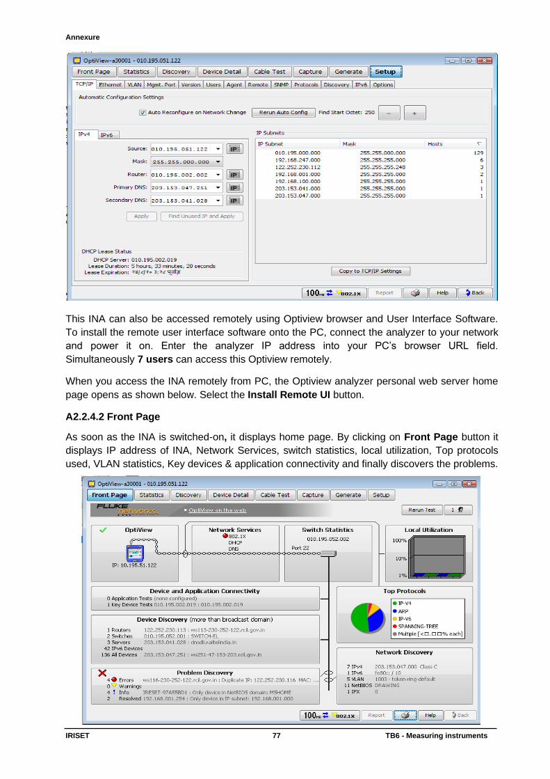
Annexure
IRISET 77 TB6 - Measuring instruments
This INA can also be accessed remotely using Optiview browser and User Interface Software.
To install the remote user interface software onto the PC, connect the analyzer to your network
and power it on. Enter the analyzer IP address into your PC’s browser URL field.
Simultaneously 7 users can access this Optiview remotely.
When you access the INA remotely from PC, the Optiview analyzer personal web server home
page opens as shown below. Select the Install Remote UI button.
A2.2.4.2 Front Page
As soon as the INA is switched-on, it displays home page. By clicking on Front Page button it
displays IP address of INA, Network Services, switch statistics, local utilization, Top protocols
used, VLAN statistics, Key devices & application connectivity and finally discovers the problems.
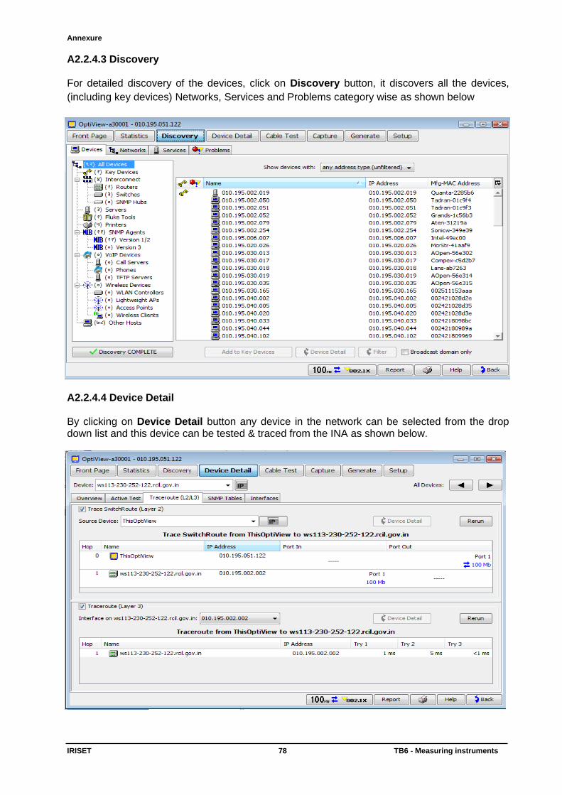
Annexure
IRISET 78 TB6 - Measuring instruments
A2.2.4.3 Discovery For detailed discovery of the devices, click on Discovery button, it discovers all the devices,
(including key devices) Networks, Services and Problems category wise as shown below
A2.2.4.4 Device Detail By clicking on Device Detail button any device in the network can be selected from the drop down list and this device can be tested & traced from the INA as shown below.
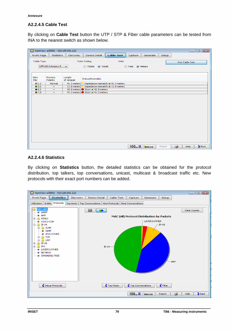
Annexure
IRISET 79 TB6 - Measuring instruments
A2.2.4.5 Cable Test By clicking on Cable Test button the UTP / STP & Fiber cable parameters can be tested from
INA to the nearest switch as shown below.
A2.2.4.6 Statistics By clicking on Statistics button, the detailed statistics can be obtained for the protocol
distribution, top talkers, top conversations, unicast, multicast & broadcast traffic etc. New
protocols with their exact port numbers can be added.
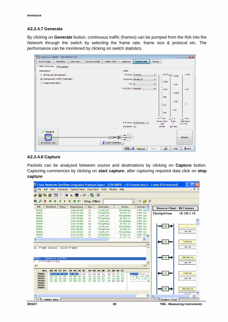
Annexure
IRISET 80 TB6 - Measuring instruments
A2.2.4.7 Generate
By clicking on Generate button, continuous traffic (frames) can be pumped from the INA into the
Network through the switch by selecting the frame rate, frame size & protocol etc. The
performance can be monitored by clicking on switch statistics.
A2.2.4.8 Capture
Packets can be analyzed between source and destinations by clicking on Capture button.
Capturing commences by clicking on start capture, after capturing required data click on stop
capture
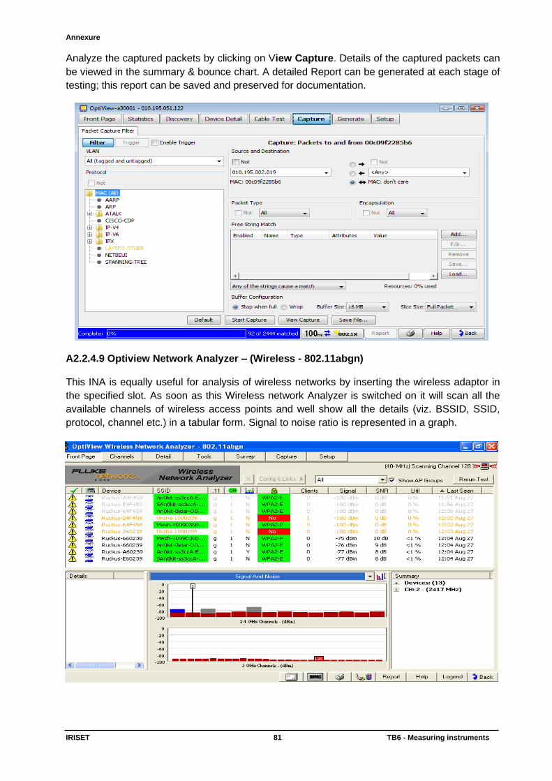
Annexure
IRISET 81 TB6 - Measuring instruments
Analyze the captured packets by clicking on View Capture. Details of the captured packets can
be viewed in the summary & bounce chart. A detailed Report can be generated at each stage of
testing; this report can be saved and preserved for documentation.
A2.2.4.9 Optiview Network Analyzer – (Wireless - 802.11abgn) This INA is equally useful for analysis of wireless networks by inserting the wireless adaptor in
the specified slot. As soon as this Wireless network Analyzer is switched on it will scan all the
available channels of wireless access points and well show all the details (viz. BSSID, SSID,
protocol, channel etc.) in a tabular form. Signal to noise ratio is represented in a graph.
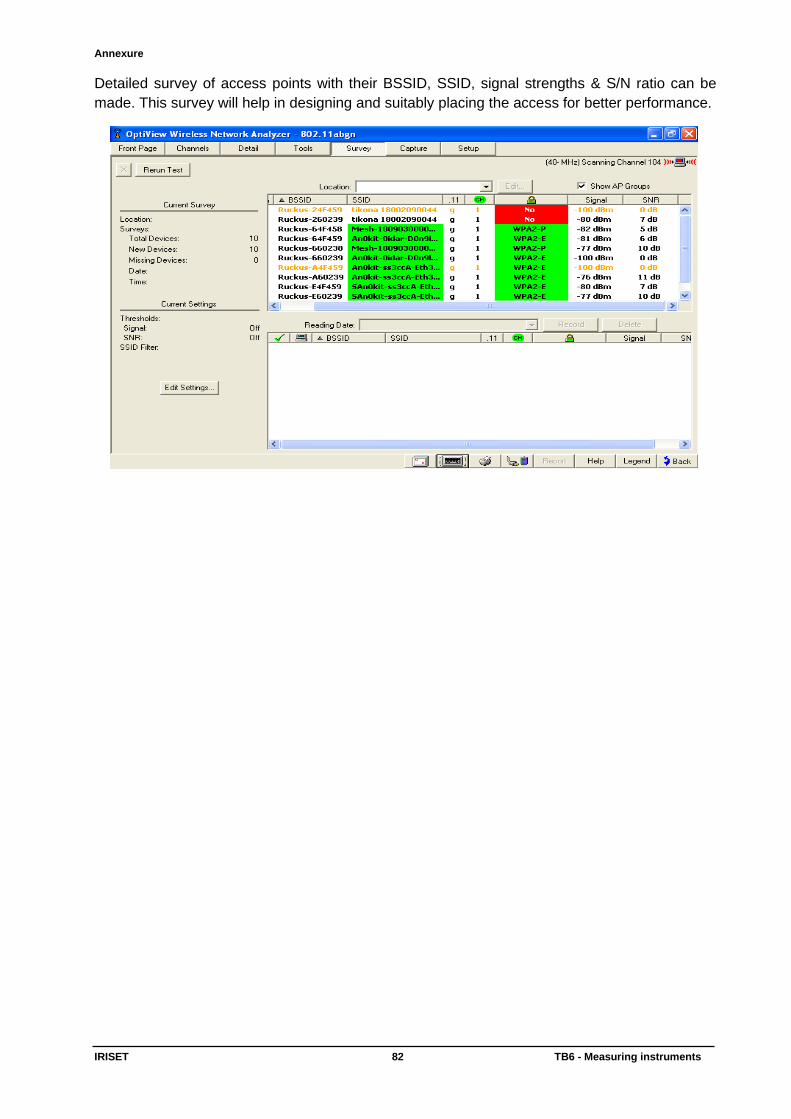
Annexure
IRISET 82 TB6 - Measuring instruments
Detailed survey of access points with their BSSID, SSID, signal strengths & S/N ratio can be
made. This survey will help in designing and suitably placing the access for better performance.
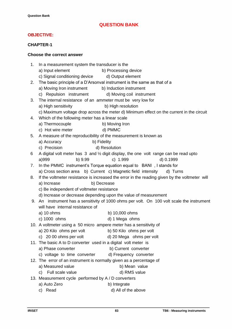
Question Bank
IRISET 83 TB6 - Measuring instruments
QUESTION BANK OBJECTIVE: CHAPTER-1 Choose the correct answer
1. In a measurement system the transducer is the
a) Input element b) Processing device
c) Signal conditioning device d) Output element
2. The basic principle of a D’Arsonval instrument is the same as that of a
a) Moving Iron instrument b) Induction instrument
c) Repulsion instrument d) Moving coil instrument
3. The internal resistance of an ammeter must be very low for
a) High sensitivity b) High resolution
c) Maximum voltage drop across the meter d) Minimum effect on the current in the circuit
4. Which of the following meter has a linear scale
a) Thermocouple b) Moving Iron
c) Hot wire meter d) PMMC
5. A measure of the reproducibility of the measurement is known as
a) Accuracy b) Fidelity
c) Precision d) Resolution
6 A digital volt meter has 3 and ½ digit display, the one volt range can be read upto
a)999 b) 9.99 c) 1.999 d) 0.1999
7. In the PMMC instrument’s Torque equation equal to BANI , I stands for
a) Cross section area b) Current c) Magnetic field intensity d) Turns
8. If the voltmeter resistance is increased the error in the reading given by the voltmeter will
a) Increase b) Decrease
c) Be independent of voltmeter resistance
d) Increase or decrease depending upon the value of measurement
9. An instrument has a sensitivity of 1000 ohms per volt. On 100 volt scale the instrument
will have internal resistance of
a) 10 ohms b) 10,000 ohms
c) 1000 ohms d) 1 Mega ohms
10. A voltmeter using a 50 micro ampere meter has a sensitivity of
a) 20 Kilo ohms per volt b) 50 Kilo ohms per volt
c) 20 00 ohms per volt d) 20 Mega ohms per volt
11. The basic A to D converter used in a digital volt meter is
a) Phase converter b) Current converter
c) voltage to time converter d) Frequency converter
12. The error of an instrument is normally given as a percentage of
a) Measured value b) Mean value
c) Full scale value d) RMS value
13. Measurement cycle performed by A / D converters
a) Auto Zero b) Integrate
c) Read d) All of the above
Question Bank
IRISET 84 TB6 - Measuring instruments
Write True or false-
14. Decibal measurement of power is a purely absolute value and dBm measurement is
a relative value……………………………………………………….. (False)
15. Dual slope integration meters are capable of rejecting noise and their accuracy is
independent of clock and time constant…………………………………………… (True)
16. The resolution of a DVM with four digits is 1 % …………………………………….. (False)
17. Moving coil instruments can be used for both AC and DC applications. …. (False)
18. Calibration of the work standard instruments are done with instruments having Primary
reference standard . …………………………………………………………………. (False)
19. Integrated circuit no. 7106 belongs to the family of A / D converters… (True)
20. A shunt in an ammeter is a resistance connected across the meter to decrease the range.
(False)
CHAPTER-2
Choose the correct answer
1. The unit of absolute power in logarithmic value of an electrical signal is –
a) dBm b) dBr c) dB d) dBrnc
2. The power output of a amplifier is +30dBm, if the power output is made double, the value
of the output power is –
a) +33dBm b)+27dBm c)+60dBm d) -30 dBm
3. If the power input of an amplifier is 1nW and the gain of the amplifier +60dB, the output
power of the amplifier is given -
a) +33dBm b)+27dBm c)+60dBm d) 0dBm
4. The Return Loss of a line is the ratio of the power reflected back from the line to the power
transmitted into the line This is due to –
a) Impedance Miss match between source and cable
b) Impedance Miss match between cable and load
c) Impedance Miss match among source and load
d) Impedance mismatch, due to changes in characteristic impedance of cable at joints
5. Bridge megger is used for -
a) Identification of low insulation fault in the cable.
b) Finding loop resistance of cable pair.
c) Contact faults within the cable pairs.
d) All of the above
6. Ac voltage is required for earth testing because of ---------------------nature of earth.
a) Resistive b) Electrolytic c) capacitive d) inductive
7. Psophometric.voltage is a …………….. measurement of noise present on a
transmission line across a telephone in mili volts.
a) lograthamic b) Linear c) Indirect d) Reverse
8. The deflection In Megger meter is determined by the ………………of current in Current
and Potential coils.
a) lAddition b) Product c) Ratio d) Reverse
State True or False
9. The loop resistance of a faulty cable reads 600 on a bridge megger at bridge position
and 400 at Varley position. The loop resistance of the cable pair is 56 / Km. The
distance of fault is calculated at 3.57km from testing point. (True)
Question Bank
IRISET 85 TB6 - Measuring instruments
10. When the reference power is one mill watt and impedance of transmission line is 600
Ohms, the equivalent reference voltage is 0.775V. (True )
11. Near end cross talk is much weaker than the far end cross talk. (False)
12. Crosstalk is the result of resistive coupling between parallel running conductors of the
cable . (False)
13. Time Domain Reflectometers are sensitivity to impedance variations, (True)
14. In the case of open or break fault in the cable, the reflection pulse in pulse echo meter will
be indicated by downward kink or negative reflection. (True)
15. In pulse echo meter, the accuracy of distance to fault depends upon the accuracy of V/2
values. (True )
16. For maximum power transfer the return loss should be as small as possible. (True)
CHAPTER-3
Choose the correct answer
1. Visual fault locator allows ____________ identification of fiber cable faults as breaks,
micro or macro bending.
a) Detailed b) Differed c) Instant d) delayed
2. VFL uses a bright ___________ colour light beam of 650nm or 635nm to inject into
the .fiber that allows to see a break as a glowing or blinking light
a) Yellow b) UV c) RED d) Blue
3. OTDR can be characterized similar to optical ____________ .
a) Radar b) Sonar c) Detector d) Amplifier
4. ………………………reflection is tens of thousands of times greater in power level than the
backscatter.
a) Internal b) Fresnel c) Total d) External
5. Pulse width is the width of the optical pulse from the OTDR that is …………………..in a
time frame.
a) scattered b) refracted c) Reflected d) generated
6. Optical Light Source provides with an inbuilt optical attenuator, to vary the attenuation of
the output level typically …………………………………..in 0.1 steps.
a) -3 to -6dB b) 0dB c) 0-6 dB d) 6-10 db
7. Optical time domain reflectometry is also called as backscatter measurement method. State whether the given statement is true or false. …………………….. 8. Which pulse width do I use to troubleshoot a long fiber run on an OTDR ? a)Longest b)Unchanged c) Medium d)Shortest
9. Are “Echo” or “Ghost” event on an OTDR trace the same . State true or false. 10. Device used to test a fiber optics splice loss is
a). Spectrum analyzer b). Oscilloscope c). Optical power meter d). Field strength meter
SUBJECTIVE:
CHAPTER-1
1. What are the elements that constitute a measuring instrument?
2. Why “ d “Arsonval movement is important for analog voltmeters ?

Question Bank
IRISET 86 TB6 - Measuring instruments
3. Define Sensitivity. How is FSD related to it?
4. Explain the advantage of using high input impedance meters?
5. Draw and explain with blocks a Digital Multi meter.
6. Explain the significance of Analog to Digital converter in a digital instrument.
7. What are the essential qualities of a good instrument?
8. Explain the importance of calibration of measuring instruments.
9. Which are the most used measuring units in telecommunication systems? Mention any
five absolute and relative measuring units
10. Write advantage and disadvantage of moving coil meter.
11. What is the difference between sensitivity and resolution of a measuring meter?
12. What is the difference between single slope digital voltmeter and dual slope digital
voltmeter?
13. How the unknown resistance value is measured with a digital multimeter? Explain with a
diagram .
CHAPTER-2
1. What are the different tests done on UG telecommunication cables?
2. What are the different faults on UG telecommunication cables, and how is Megger useful
in testing them?
3. State the principle of Cable route tracing?
4. Explain how cable fault location can be done through Time Domain Reflectrometer
method?
5. State the principle of Digital earth resistance tester?
6. Describe the method of measurement of earth resistance.
7. Explain how Transmission measuring sets are useful for testing voice frequency
telephone systems? State different tests.
8. Differentiate between Return loss and Insertion loss.
9. Describe the principle of SLM, What are the tests that can be done with a SLM?
10. What are the functions of pulse echo meter? Write down the procedure of finding the
cable faults with the pulse echo meter.
11. What is the functional difference between pulse echo meter and bridge megger?
12. What is the utility of guarding the terminals in megger? Explain with the few lines.
13. What are the basic differences between the insulation test megger and earth test megger?
Explain briefly.
14. Can you use a simple ammeter and a voltmeter with a DC voltage source to measure
earth resistance of an installed earth electrode? If not what meter you like to use and
why?
15. Explain the procedure of testing the earth resistance of a earthed electrode of a
installation with the null balance earth test megger.
16. What is near-end cross talk and far-end cross talk in the cable? Explain with a block
diagram. .
17. What is the difference between the wide band and selection band of the selective level
meter? Mention the frequency range of wide band and selection band.
18. Why calibration is required when measuring any signal level and how the calibration is
done before any measurement?.
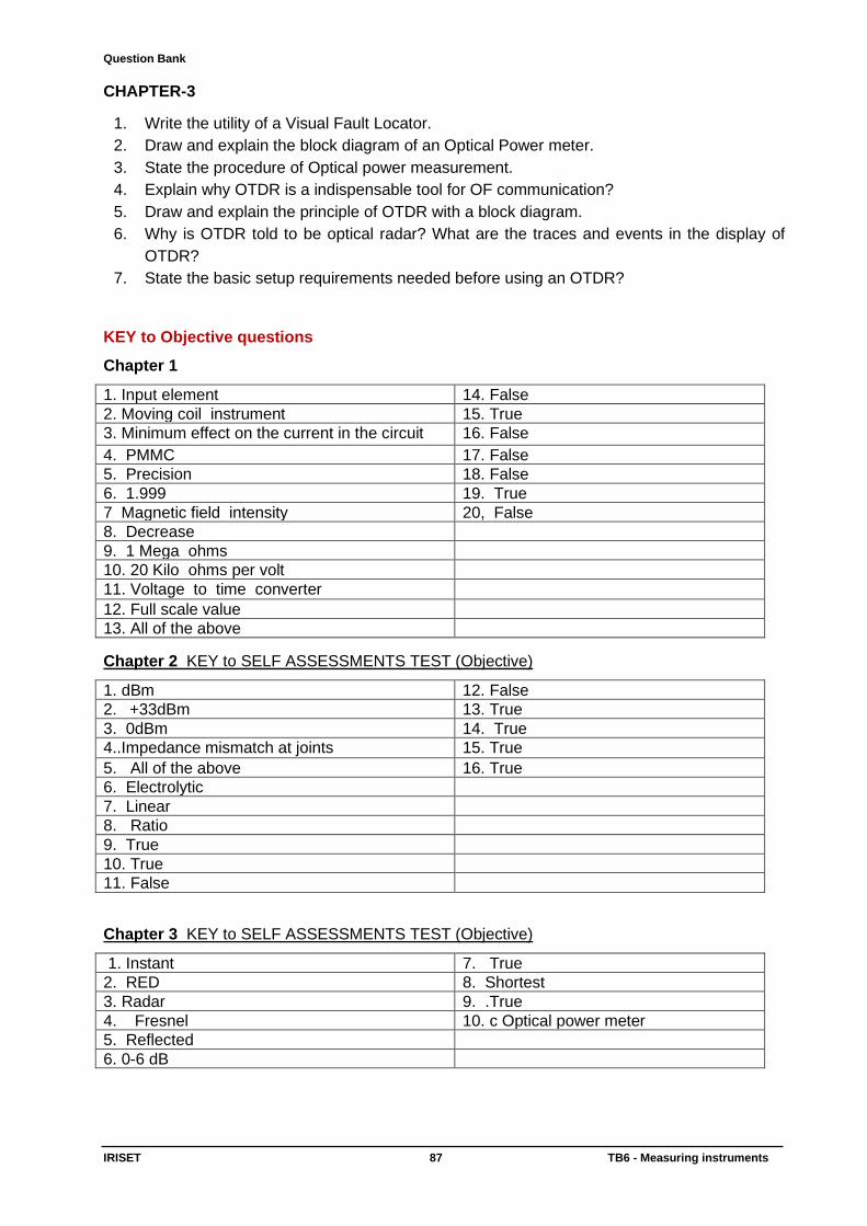
Question Bank
IRISET 87 TB6 - Measuring instruments
CHAPTER-3
1. Write the utility of a Visual Fault Locator.
2. Draw and explain the block diagram of an Optical Power meter.
3. State the procedure of Optical power measurement.
4. Explain why OTDR is a indispensable tool for OF communication?
5. Draw and explain the principle of OTDR with a block diagram.
6. Why is OTDR told to be optical radar? What are the traces and events in the display of
OTDR?
7. State the basic setup requirements needed before using an OTDR?
KEY to Objective questions
Chapter 1
1. Input element 14. False
2. Moving coil instrument 15. True
3. Minimum effect on the current in the circuit 16. False
4. PMMC 17. False
5. Precision 18. False
6. 1.999 19. True
7 Magnetic field intensity 20, False
8. Decrease
9. 1 Mega ohms
10. 20 Kilo ohms per volt
11. Voltage to time converter
12. Full scale value
13. All of the above
Chapter 2 KEY to SELF ASSESSMENTS TEST (Objective)
1. dBm 12. False
2. +33dBm 13. True
3. 0dBm 14. True
4..Impedance mismatch at joints 15. True
5. All of the above 16. True
6. Electrolytic
7. Linear
8. Ratio
9. True
10. True
11. False
Chapter 3 KEY to SELF ASSESSMENTS TEST (Objective)
1. Instant 7. True
2. RED 8. Shortest
3. Radar 9. .True
4. Fresnel 10. c Optical power meter
5. Reflected
6. 0-6 dB
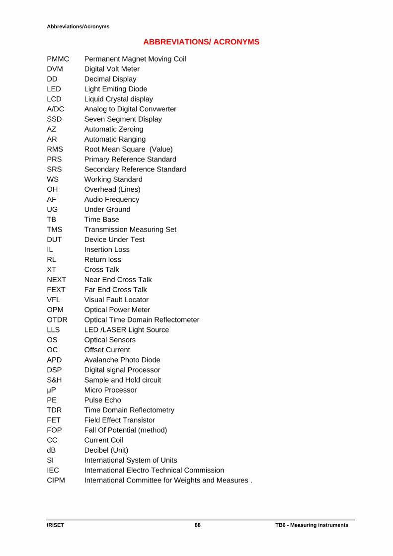
Abbreviations/Acronyms
IRISET 88 TB6 - Measuring instruments
ABBREVIATIONS/ ACRONYMS PMMC Permanent Magnet Moving Coil
DVM Digital Volt Meter
DD Decimal Display
LED Light Emiting Diode
LCD Liquid Crystal display
A/DC Analog to Digital Convwerter
SSD Seven Segment Display
AZ Automatic Zeroing
AR Automatic Ranging
RMS Root Mean Square (Value)
PRS Primary Reference Standard
SRS Secondary Reference Standard
WS Working Standard
OH Overhead (Lines)
AF Audio Frequency
UG Under Ground
TB Time Base
TMS Transmission Measuring Set
DUT Device Under Test
IL Insertion Loss
RL Return loss
XT Cross Talk
NEXT Near End Cross Talk
FEXT Far End Cross Talk
VFL Visual Fault Locator
OPM Optical Power Meter
OTDR Optical Time Domain Reflectometer
LLS LED /LASER Light Source
OS Optical Sensors
OC Offset Current
APD Avalanche Photo Diode
DSP Digital signal Processor
S&H Sample and Hold circuit
μP Micro Processor
PE Pulse Echo
TDR Time Domain Reflectometry
FET Field Effect Transistor
FOP Fall Of Potential (method)
CC Current Coil
dB Decibel (Unit)
SI International System of Units
IEC International Electro Technical Commission
CIPM International Committee for Weights and Measures .
Reference
IRISET 89 TB6 - Measuring instruments
REFERENCE
1. Electronic Instrumentation and measurement techniques By COOPER
2. Data sheet of MEGGER (Insulation Tester)
3. Data sheet of Digital Megaohmmeter
4. Data sheet of Network Analyzers AGILENT
5. Data Sheet of RF Power Meters HEWLET PACKERD
6. Data sheet of ANT-20 ,JDSU (ACTERNA)
7. WIKIPEDIA
Glossary
IRISET 90 TB6 - Measuring instruments
GLOSSARY
A Analog 4 Automotive control 5. Aluminium frame (Spindle)5. Angular deflection 5, Alloy Metals 6, A/D converter 10,13 Automatic Zeroing 13 Automatic Ranging 14,15 Audio freq.generator26 Audio freq.receiver 26 Absolute measurement34 Antenna measurement35 B Buffer Amplifier 13 Bridge Megger 22 C Conversion element 4 Control System 4 Controlling torque 5, Continuous scale 7 Clock Pulse 14 Calibration 19 Calibration chain20 Calibration record20 Compensating Coil 22 Cable route locator 28 Capacitive coupling 27 Cable fault locator Characteristic impedance29 31 Crystal Oscillator32 Crosstalk Meter 44 D Display system 4 Digital 4 Discrete steps 4 De’ Arsonval movement 4 Damping torque 5 , 6 Dual Slope Ramp type converter 9 , 12 Decade counting unit 10 13 Drift in characteristics 19 Disconnection fault 21 DC generator22 Deflecting Coil 23 Digital Insulation tester 25 Digital earth Tester 31 Decibel 34 E Electro dynamics 4, Electro magnetic 5, Eddy currents 5,
Errors during measurement 17 Environmental changes18 Earth fault 21 F Finite numbers 4 flux density 6, Flying capacitor 12 Foreign potential fault 21 Foreign voltage 29 Fall off potential method 33 FEXT 46 G Galvanometer 4 ,5 7 Galvanometer sensor4 Galvanometer deflection 24 Galvanic coupling 27 Guidance Arrow27 H Hysteresis 7, Highly sensitive and selective Receiver 26 I Infinite 4 Integrator 10, Insulation resistance 21 Indiscriminate digging 25 Inductive coupling 27 Impedance Disturbance 30 Insertion loss 36 J Jewelled Bearing 5 L LCD seven segment 13, Linearity 17 Lag Set Timings17 Limitation of measuring instruments 20 low insulation Fault21 LED/LASER light Source 49 M Measuring instruments 4, Measuring Systems 4 Moving Coil 4 Moving iron 4 Multitasking 143 Measurement (AZ/INTEG/READ/AZ ) cycle 15 Measurement period 15 Megger 22 Murray loop test 24 Mapping display 27
Glossary
IRISET 91 TB6 - Measuring instruments
N Noise and integration over Time 11 National Standard Organization 20 Noise 21 Noise Measurement 40 Noise power in decibels 41 NEXT 46 Non Reflection events43 O Observational errors 8 Ohm meter 31 Optical Power Meter 48 OTDR 50 OTDR setup 51 P Permanent magnet 5, Portability 7. Pulse generator 9 Precision17 Protection resistance 22 Proximity signal 27 Pulse reflection Principle 28 Pulse echo method 28 Psophometric voltage41 Psophometer 41 Psophometrically weighted noise 42 R Resistance Shunt 6, Rectangular pulse 9 Rise and Fall 9, Ramp generator 9 10 RC Time constant12 Resolution 17 Range17 Repeatability 17 Reproducibility Random Errors 18 Random excavation 25 Return loss 36 Reflection Coefficient 39 Reflection events 42 S Sensor 4 Signal Recording unit 4 ,5 Single Slope Ramp type converter 10 Sample rate Multivibrator 10 Sample and Hold 12 Sensitivity 16, System Disturbance 18 Short Circuit fault 21 Search coil 26 Sensor 26, Synchronous Filtering 32
T Tele Communication systems 4, Trigger (+/=) 9 Train Pulses 9 Transducers 5, Temperature Coefficients 6, Time base 10 Time Interval Counter 10 Time domain Reflectometry 28 , 30 Terminating resistance 30 Transmission measuring set 36 Transmission Loss Measurement 37 Trace analysis of OTDR 41 U Up down converter 14 Universal earth tester 31 V Versatility and accurate 7 Varley Loop Test 25 Velocity of propagation 29 Visual Fault Locator 46 W Wheat stone bridge 24
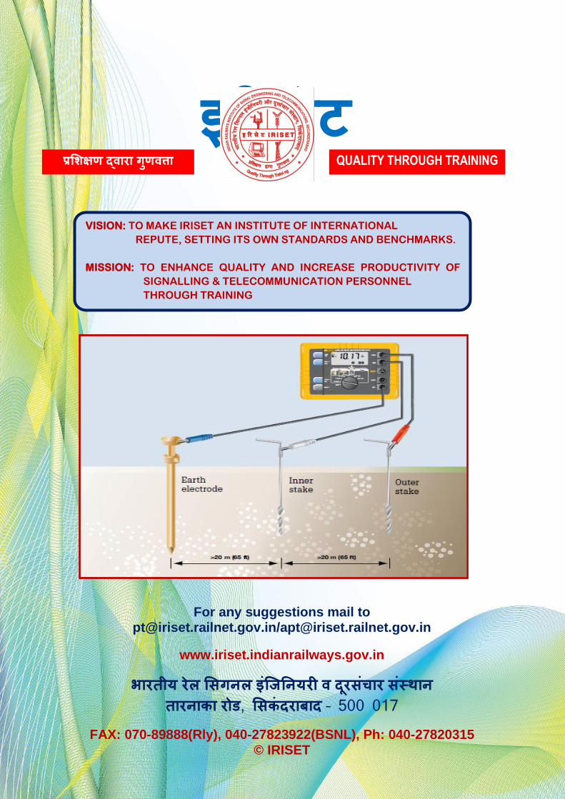
इरिसट IRISET
VISION: TO MAKE IRISET AN INSTITUTE OF INTERNATIONAL
REPUTE, SETTING ITS OWN STANDARDS AND BENCHMARKS.
MISSION: TO ENHANCE QUALITY AND INCREASE PRODUCTIVITY OF
SIGNALLING & TELECOMMUNICATION PERSONNEL
THROUGH TRAINING
For any suggestions mail to [email protected]/[email protected]
www.iriset.indianrailways.gov.in
भाितीय िल ससगनल इजिननयिी व दिसचाि ससथान तािनाका िोड, ससकदिाबाद – 500 017
FAX: 070-89888(Rly), 040-27823922(BSNL), Ph: 040-27820315
© IRISET
QUALITY THROUGH TRAINING परसिकषण दवािा गणवतता


![INDEX [122.252.230.113]122.252.230.113/content/notes/sig/S24.pdf · 2018. 3. 7. · SL.NO CHAPTER PAGE NO 1. Intermediate Block Signalling 1 2. Axle Counter Block working 20 3. Block](https://img.pdfslide.us/doc/110x75/6103ea46fa925019910f8672/index-122252230113122252230113contentnotessigs24pdf-2018-3-7.jpg)


![WELCOME [122.252.230.113]122.252.230.113/content/ppt/tele/TB_1hl.pdfQuality improvement through training. 2. Practical Approach of Learning. 3. Signalling and Telecommunication Safety](https://img.pdfslide.us/doc/110x75/613e1d8c59df64284616537d/welcome-122252230113122252230113contentpptteletb1hlpdf-quality-improvement.jpg)


![INDEX [122.252.230.113]](https://img.pdfslide.us/doc/110x75/61e333495ac58c138b538d23/index-122252230113.jpg)