649

internal

report

Ranger Trial Landform:

Hydrology – Standard

Operating Procedures

for Erosion Plot Data

Management

J Boyden, M Saynor and

M Rudge

October 2016

Release status – unrestricted

Project number – RES-2009-011

The Department acknowledges the traditional owners of country throughout Australia and their continuing

connection to land, sea and community. We pay our respects to them and their cultures and to their elders

both past and present.

Ranger Trial Landform: Hydrology – Standard Operating Procedures for Erosion Plot Data

ManagementJames Boyden, Mike Saynor and Mitch Rudge

Supervising ScientistGPO Box 461, Darwin NT 0801

October 2016

Release status – unrestricted

How to cite this report:

Boyden J, Saynor M & Rudge M 2016. Ranger Trial Landform: Hydrology – Standard Operating Procedures for Erosion Plot Data Management. Internal Report 649, October, Supervising Scientist, Darwin.

Project number: RES-2009-011

Authors of this report:

James Boyden –Supervising Scientist, GPO Box 461, Darwin NT 0801, AustraliaMike Saynor –Supervising Scientist, GPO Box 461, Darwin NT 0801, AustraliaMitch Rudge –Supervising Scientist, GPO Box 461, Darwin NT 0801, Australia

The Supervising Scientist is a branch of the Australian Government Department of the Environment and Energy.Supervising ScientistDepartment of the Environment and EnergyGPO Box 461, Darwin NT 0801 Australiaenvironment.gov.au/science/supervising-scientist/publications

© Commonwealth of Australia 2016

IR649 is licensed by the Commonwealth of Australia for use under a Creative Commons By Attribution 3.0 Australia licence with the exception of the Coat of Arms of the Commonwealth of Australia, the logo of the agency responsible for publishing the report, content supplied by third parties, and any images depicting people. For licence conditions see: http://creativecommons.org/licenses/by/3.0/au/ DisclaimerThe views and opinions expressed in this publication are those of the authors and do not necessarily reflect those of the Australian Government or the Minister for the Environment and Energy.While reasonable efforts have been made to ensure that the contents of this publication are factually correct, the Commonwealth does not accept responsibility for the accuracy or completeness of the contents, and shall not be liable for any loss or damage that may be occasioned directly or indirectly through the use of, or reliance on, the contents of this publication.

ContentsExecutive summary v

List of figures vi

List of tables vii

1 Introduction 1

2 Data management methods 52.1 Data editing 12.2 Data quality codes 3

3 Rainfall data correction methods 5

4 Shaft encoder stage trace correction Part I: general methods 74.1 Calibration of stage trace to CTF 74.2 Data labels and comments added to selected data points 24.3 Consistency checks 34.4 Infilling of missing stage height data 44.5 Rainfall vs runoff summary reporting 5

5 Shaft encoder stage trace correction Part II: site-specific issues 75.1 Boundary overflow 7

5.1.1 Comparing different site stage traces to correct for overflow 7

5.1.2 Estimated contribution of ‘overflow’ to runoff measured from EP1 9

5.2 Evaluating accuracy of shaft encoder measurements at high flows 9

6 References 11

Appendix 1 – Data reporting methods 12A1.1 Generating standardised comments reports 12A1.2 Summarise discharge for individual events using a standardised

spreadsheet template 13A1.2.1 Run HYCRSUM to convert stage height (100.01) to total volume

(153.01) in Litres. 15

A1.2.2 Calculate runoff volume for discrete events over one wet season 18

A1.3 Apply HYEXTREM to check number of discrete events in spreadsheet summary 23

iii

Executive summaryThis report outlines the Standard Operating Procedures (SOPs) for management, quality assessment and corrections applied to the hydrology data gathered from Erosion Plots (EP) of the Ranger Trial Landform. These time-series datasets are to be used in conjunction with other measured variables to: a) determine physical erosion rates in relation to rainfall and surface water discharge; b) provide calibration input data for predictive geomorphic computer modelling of proposed landform designs (Lowry et al 2015); and c) determine contaminant loads, pathways, and sedimentation sinks. The SOPs cover data collection and management methods, general checking and correction methods, shaft encoder stage trace correction and data reporting methods. As such, the SOPs provide a basis to attain consistent standards in data quality that are suitable for intended purposes of the data. The SOPs also support a series of reports on the corrected trial landform hydrology datasets that are written, as required, for selected plots and periods; for example, see Saynor et al. (2016) and Boyden et al. (2016).

List of figuresFigure 1 The location of Ranger uranium mine in the Alligator

Rivers Region..............................................................................1Figure 2 Aerial view of the completed trial landform with 30 x 30

m Erosion Plots (EP1 to EP4)......................................................2Figure 3 Erosion Plot (EP1) showing the boundary pipe, stilling

basin, flume and downstream basin drain. The adjacent roadside drain of EP1 (top left) is also shown. Photo taken December 2009...........................................................................3

Figure 4 Screenshot from the Hydstra Data Managers workbench with data editing workflow for TLF1 overlayed..........................1

Figure 5 Example of how a comment is added to a selected point at end of an edited data series from the “edit data point” window of Hydstra DMWB..........................................................3

Figure 6 Example of screenshot report of cumulative rainfall for the 2009–2010 wet season (total 1533 mm) from EP1..............6

Figure 7 A labelled screenshot from the Hydstra editing window showing the water level of the primary trace (variable 100.01, blue line) and a standardised series of comment tags (italics) for two types of events (Basin fill only and runoff over flume). The Hydstra ‘©’ label indicates point records with comments entered during editing. The CTF calibration line in this example is for EP1.......................................................................1

Figure 8 Example of access to standardised comments via the “add standard comment” button of the Hydstra MWB ‘Edit data point’ window..............................................................................2

Figure 9 Example of how a time-offset correction for EP1 was determined by comparing difference in rainfall traces for all sites.............................................................................................4

Figure 10 Evidence and correction of roadside drain overflow event where: a) overflow is indicated by a 2nd peak in the EP1 trace after a brief yet intense 31 mm rain event on the 21st December 2011; and b) correction applied to abnormal records by manual editing (orange line)..................................................8

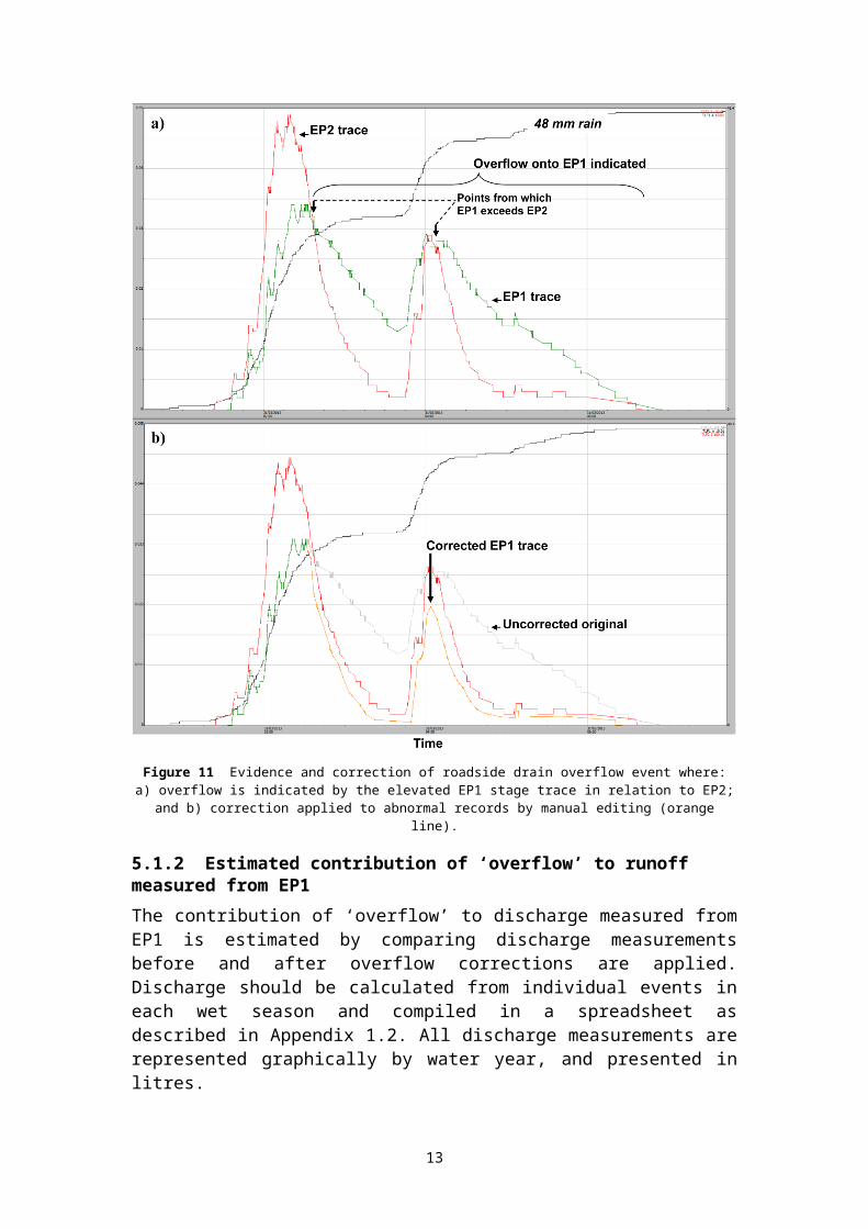
Figure 11 Evidence and correction of roadside drain overflow event where: a) overflow is indicated by the elevated EP1 stage trace in relation to EP2; and b) correction applied to abnormal records by manual editing (orange line).....................................9

Figure 12 Example of water-level disturbance in the upstream stilling basin at EP2 during the peak of a high-flow event. This turbulence is expected to cause the shaft encoder to underestimate water level.........................................................10

List of tablesTable 1 List of pre-season checks to be undertaken at each

erosion plot site before commencement of wet season monitoring...................................................................................1

Table 2 General description of runoff and rainfall related variables names as stored in Hydstra.........................................................2

Table 3 Data quality codes used to described rainfall and runoff data records.................................................................................4

Table 4 Example of rainfall report of corrected wet season rainfall totals for an erosion plot site (EP1).............................................6

Table 5 Example of missing data report for erosion plots and how these data gaps were infilled.......................................................5

1 IntroductionThe Ranger uranium mine (Figure 1) is located in the Alligator Rivers Region in the wet-dry monsoonal tropics, approximately 250 km east of Darwin, Northern Territory. A collaborative research program involving the Supervising Scientist Branch and mine operator Energy Resources of Australia (ERA), has been underway to measure, from a trial rehabilitation landform, long-term (five to ten year), rates of erosion and contaminant transport under different surface treatments and vegetation establishment regimes. The trial landform of approximately 200 m by 400 m (8 ha) was constructed during late 2008 and early 2009 by ERA, adjacent to the north-western wall of the tailings storage facility at the Ranger Mine (Figures 1 & 2). To support this research, four Erosion Plots (EPs) were built on the landform during 2009 by the Supervising Scientist Branch (nominally designed to be 30 m X 30 m, 900 m2 in area and constructed on a 2 % slope) to continuously monitor, across the different regimes: rainfall; associated surface water runoff; and solute and sediment transport (suspended sediment and bedload).

1

Figure 1 The location of Ranger uranium mine in the Alligator Rivers Region

2

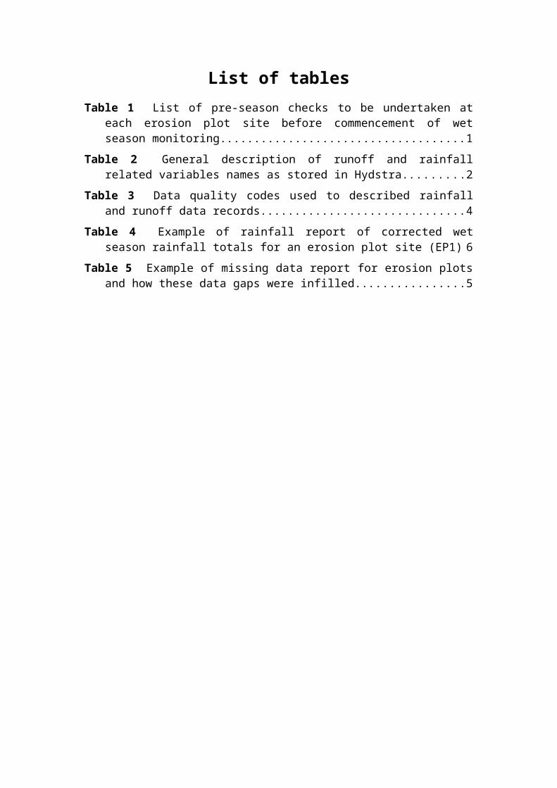
Figure 2 Aerial view of the completed trial landform with 30 x 30 m Erosion Plots (EP1 to EP4).

The erosion plot containment boundaries were dampcourse concreted in place with u-PVC pipe at the downstream end of each plot. The pipe is sloped (>0.02 m/m) toward one side of the plot to divert water into a stilling basin upstream of a RBC flume  (Bos et al 1984, Clemmens et al 2001). Stage height of surface water leaving the plot is measured by two sensors: a Unidata optical shaft encoder, model 6541C-11C (the primary sensor) in a stilling well with the intake in the stilling basin; and a GE Druck PTX 1830 pressure transducer (the secondary sensor) with the intake in the upstream section of the flume and range of 0.79 to 1.5m H2O gauge.

Rainfall is measured at 1-minute intervals from each plot using a 0.2 mm tipping bucket rain gauge (TB3 model by Hydrological Services Pty. Ltd.). The four rain gauges are cleaned and calibrated towards the end of each dry season. They are located just down-slope of each plot, for example as shown for EP1 in Figure 3. Data for rainfall and runoff are recorded by a data logger (CR1000, Campbell Scientific) at 1-min and 10-s intervals, respectively. If no value change is detected for a given variable in the measurement interval periods then no data record is logged. These data are uploaded on a daily basis via a telemetry link to a time-series database used for storing hydrologic information (Hydstra version 10.2.2, http://kisters.com.au/).

3

EP1EP2

EP3EP4

Tailings Storage Facility

Figure 3 Erosion Plot (EP1) showing the boundary pipe, stilling basin, flume and downstream basin drain. The adjacent roadside drain of EP1 (top left) is also shown. Photo taken December 2009.

Erosion Plot (EP) measurements are logged only when a sensor indicates change from the last measurement interval. Physical characteristics of each erosion plot are to be described in detail in the data quality reports produced for each plot site. Background information is also provided in Saynor et al. (2013).The EP time-series datasets for rainfall and runoff are to be used in conjunction with other measured variables to: a) determine physical erosion rates in relation to rainfall and surface water discharge; b) provide calibration input data for predictive geomorphic computer modelling of proposed landform designs (Lowry et al 2015); and c) determine contaminant loads, pathways, and sedimentation sinks. To meet these requirements, the hydrology datasets must first undergo rigorous screening and editing to provide assurance that data were suitable for intended purposes. In this regard, this report provides the Standard Operating Procedures (SOPs) for management, quality assessment and corrections applied to the hydrology data gathered from erosion plots of the Ranger Trial Landform (TLF). The SOPs cover data management methods, correction methods, shaft encoder stage trace corrections and data reporting methods. The SOPs also support a series of reports on the corrected trial landform hydrology datasets that are written, as required, for selected plots and periods; for example, see Saynor et al. (2016) and Boyden et al. (2016).

4

This SOPs are in a controlled (live) document that is to be updated with additional information as required. The electronic version will be reviewed annually to check whether changes are necessary. Any changes to the SOP will be listed within the ‘Record of Revisions’ section on page iii of this electronic document. The controlled SOP is stored on SPIRE (the Department’s electronic document management system) under: Supervising Scientist > Management and Administration > Laboratory and Sample Management >Manuals and Procedures > HGCP – Procedures Manual.Fully processed hydrology data, having undergone quality checks and correction, are to be reported in the SSB Internal report series by each plot (EP1 to EP4) and each water-year, separately. Importantly, a water-year is defined as the period between 1 September and 31 August the following year. The objective of this exercise is to attain a complete and accurate rain and runoff record for each plot and water-year period. This is achieved by:a) Checking consistency and completeness of data for each erosion

plot and water-year period; b) Systematically applying data corrections; and if gaps in the

continuous record exist c) Applying data substitution from a suitable alternative data

source, when available, as collected from other monitoring sites of the TLF.

Once a site’s dataset is cleaned and deemed complete for a water-year monitoring period1 it is to be reported in a series of internal data reports for each site. Each report will state the plot name (e.g. EP1) and the data coverage period in complete water-years (and of at least one complete water-year).The corrected and uncorrected (original) EP hydrology datasets are stored and managed in the time-series database system for hydrologic information, Hydstra version 10.2.2 (see http://kisters.com.au/). This database is located in the Darwin office at HYDSTRA$(\\pvnt01flpr01)(U:)\HYD. New data are checked and edited for consistency and completeness using the Data Managers Workbench (DMWB) of Hydstra. Users of this document are expected to have a basic working knowledge of this software.

1 A water year period is nominally from 1 September to 31 August the following year.

5

2 Data management methodsEach erosion plot site will undergo pre-season maintenance, instrument function and calibration checks. General checklist requirements are described in Table 1 (next page). During each monitoring period (water-year, September – August), new hydrology records are uploaded to Hydstra on a daily basis via a telemetry link. Regular checks of the data are essential for timely detection and resolution of issues with the continuous monitoring systems. Identified site- or system-specific problems are to be communicated promptly to technicians involved in the maintenance of field equipment. Correcting and validating the consistency and completeness of the continuous time-series data involves checking records for each site (erosion plot) sensor: a) with parallel records from different sensors recorded at the same site; and b) with identical variables, also recorded in parallel at the other nearby sites. Specifically, this includes checking: The rainfall data traces for all erosion plot gauges against each

other; A site’s runoff data (i.e. stilling basin water levels), recorded

from either the shaft encoder or pressure transducer sensors, against associated rainfall data;

A site’s runoff data from either the shaft encoder or the pressure transducer sensors against corrected runoff data for another site; and

A site’s shaft encoder or the pressure transducer data against each other.

While some inherent variation between different sensors/sites is expected, distinct mismatches in data pattern are likely to indicate a data quality problem. Problems with new data may then be identified by an abrupt, gradual or occasional change in measurement values. An occasional abnormal change may be associated with episodic higher rainfall. For example, a problem with overflow across a plot’s containment boundary could be indicated by higher than normal runoff at one plot relative to another. Other types of problems can include an instrumentation malfunction (including calibration issues) or a physical issue with the erosion plot containment. Procedures undertaken to check and correct data, systematically, are described in following Sections. This process is iterative and involves using the Hydstra DMWB to work through the entire data series, several times. Editors should develop their own routines to ensure all data are checked thoroughly. They are also to maintain a spreadsheet outlining progress in working through each dataset for specific sites and variables (e.g. Appendix 1). This will allow them

6

to endorse the quality of data blocks as they are completed. Once a site dataset for an entire wet-season period is deemed complete it will be validated independently by another trained technician.

7

Table 1 List of pre-season checks to be undertaken at each erosion plot site before commencement of wet season monitoring.

Check at each erosion plot site:

1) Has there been a previous breach of the plot’s containment boundary at high runoff flows, or is there potential for one?

If yes, consider the most practical option to prevent a boundary breach, such as excavating a drainage channel to divert off-site water away from the plot site or raising the height of the boundary wall. Repairs to the containment boundary wall may also be necessary if erosion has occurred under or over the wall. Similarly, drainage channels built to divert offsite waters may have filled with sediment after each water season and therefore may need to be dug out.

2) Is the u-PVC pipe used to direct water into a stilling basin properly affixed to the concrete boundary and are there any cracks in the pipe that may allow offsite seepage?

If no, measures are required to affix the PVC pipe using sealant or other measures.

3) Is the stilling basin water-tight? If no, sealant may need to be applied.4) Is logging equipment functional? The data logger must write to the onsite data logger which can be

tested onsite by a trained technician with laptop with connection to the logger. If not functioning there could be an electrical problem such as a bad connection or battery.

5) Is modem and data transmission equipment functional?

The modem is programmed to transmit new data on a daily basis to the Darwin office computer server. If this does not happen at the specified time after data has been logged there may be a problem. However data will only transmit if no new records have been recorded (i.e. new data is logged when there has been a change from zero).

6) Are stage height sensors (shaft encoder and pressure transducer) functional and calibrated to the

If no, the problem will need trouble-shooting by a trained technician. If new sensors are required these should be bench-tested in a lab, before site installation. Calibration information supplied with new

1

Cease to Flow (CTF) line (See Section 4.1 for method)?

sensors are filed in the Darwin office. Field calibration requires that stage heights for shaft-encoder and pressure transducer be zeroed to the CTF line.

2

2.1 Data editing The hydrological datasets for the erosion plots are stored in the SS Hydstra file named TLF12 to TLF4 (Trial Land Form 1 to 4). An example of the data editing workflow undertaken in the Hydstra DMWB is shown in Figure 4 for TLF1. Original data from the field data-logger are appended to the TLF# B master file (the raw data) on a daily basis. Complete and cleaned datasets for rainfall and runoff are maintained in the M file (TLF1 and 2) or the J file (TLF3 and 4). Other files’ letters are not be used for storing the primary corrections for rain and runoff. When editing has been verified it is placed in the archive file (TLF# A).

Figure 4 Screenshot from the Hydstra Data Managers workbench with data editing workflow for TLF1 overlayed.

The rainfall and runoff variables are named by the respective numeric codes 10 and 100. A sub-decimal code signifies the level of editing and the probe type used to take the measurement (Table 2) and original data are given a zero by default (e.g. 10.00). Cleaned versions of rainfall and water level data are renamed 10.01 and 100.01, respectively.

2 TLF1 is a site alias for EP1 (Erosion Plot 1) etc.

1

Table 2 General description of runoff and rainfall related variables names as stored in Hydstra.

Variable Code name Description Editing level

Water-level (m), Variable 100

100.00 Shaft encoder sensor (primary measurement)

Raw data

100.01 Core dataset for analysis. Working draft or complete edited data with all corrections, except CTF point is not zeroed. Includes some secondary data substitutions and manual editing where required

100.02 100.02 Edited data >= CTF and zeroed to

100.10 Secondary measurement (pressure transducer)

Unedited pressure transducer data

100.11 100.11 Edited pressure transducer data

Variable calculated from 100.01

153.00 Calculated discharge (L) as derived from the 100.01 variable using conversion formulae outlined in Saynor et al. (2013). This calculation excludes discharge for residual stilling basin waters (e.g. minor runoff events into the stilling basin that do not contribute to flow over the flume directly)

Derived from 100.01. A .01 suffix to be added to indicate calculated output from cleaned 100.01 dataset

Rainfall (mm) 10.00 Tipping bucket rain gauge (0.2 mm increments)

Raw rainfall data originating from the Hydstra B file for erosion plots

10.01 10.01 Edited rainfall data originated from the Hydstra B file for erosion plots

Corrections and data descriptors are also to be recorded as concise comments linked to individual points in the data series. The comments should include the editor’s initial and date at which the change was made. For infilled data gaps the comments must also state the source of the substitute data (e.g. site name) and the method used (e.g. “direct infill”). Data gaps and corrections will be reported in a site’s data report by tabulating these details. Comments are displayed on the DMWB GUI by selecting the appropriate check-box. For quick reference their position on the data trace can be shown by a © symbol. Comments are to be placed in a logical and consistent position on the data trace with respect to the type of correction or data description. For example, a correction description should be attached to the first and last point on the portion of the data trace that the comment refers to. The first point will indicate the corrections are to the right of the trace series while the last point will indicate the corrections are to the left of the series. Comments are added via the “edit data point”

2

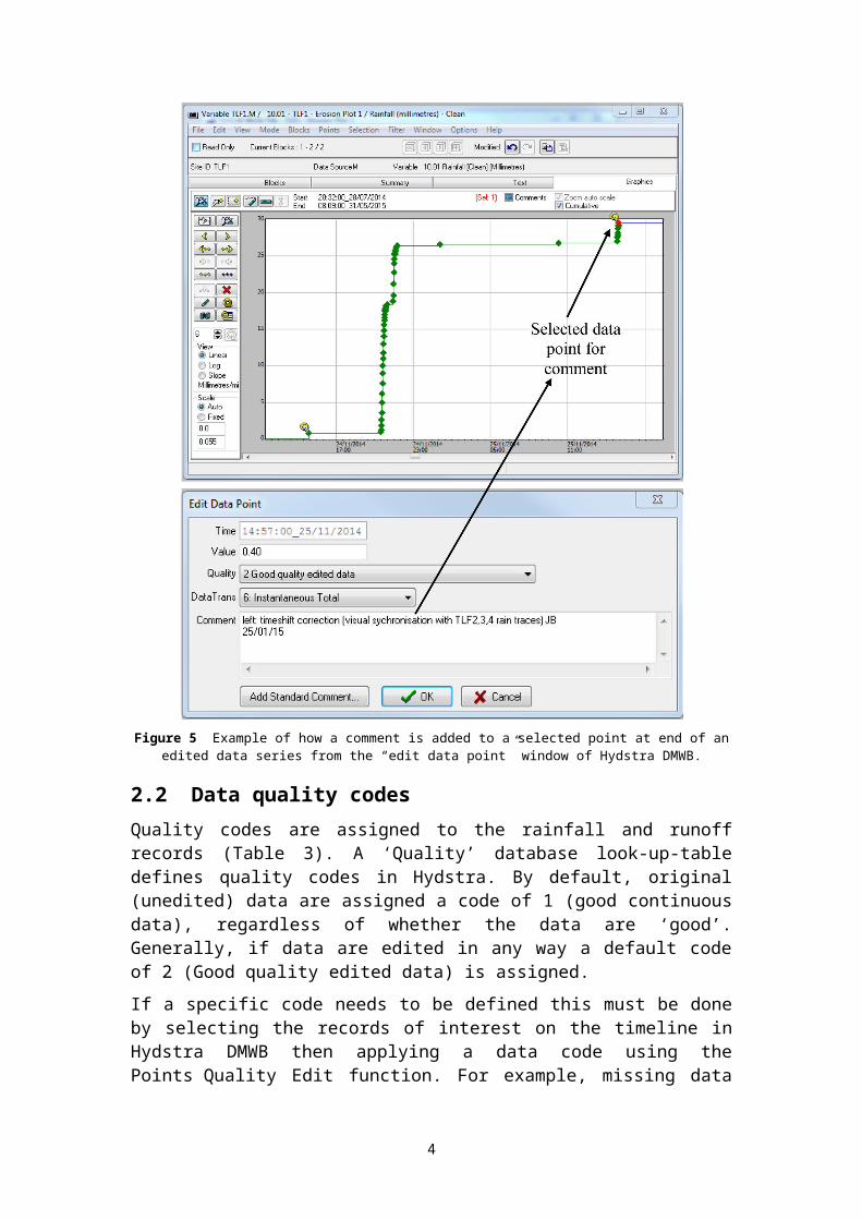
window of DMWB. This window is displayed automatically after making any change (either to a selected point or a series of points), or can be opened by double-clicking on any point. When entering a comment to a selection of points it will attach only to the first point in each continuous series of points3.When a correction is applied to a series of data points a comment is to be entered to points selected at the beginning and end of the data series. A point is selected and edited by double-clicking on it to open the “edit data point” window (e.g. Figure 5).

Figure 5 Example of how a comment is added to a selected point at end of an edited data series from the “edit data point” window of Hydstra DMWB.

2.2 Data quality codesQuality codes are assigned to the rainfall and runoff records (Table 3). A ‘Quality’ database look-up-table defines quality codes in 3 The comment can also be duplicated to multiple sets of points (i.e. the first point of

each continuous set, separated by unselected points)

3

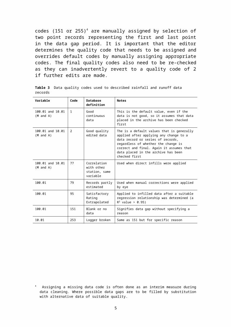
Hydstra. By default, original (unedited) data are assigned a code of 1 (good continuous data), regardless of whether the data are ‘good’. Generally, if data are edited in any way a default code of 2 (Good quality edited data) is assigned. If a specific code needs to be defined this must be done by selecting the records of interest on the timeline in Hydstra DMWB then applying a data code using the Points Quality Edit function. For example, missing data codes (151 or 255)4 are manually assigned by selection of two point records representing the first and last point in the data gap period. It is important that the editor determines the quality code that needs to be assigned and overrides default codes by manually assigning appropriate codes. The final quality codes also need to be re-checked as they can inadvertently revert to a quality code of 2 if further edits are made.

Table 3 Data quality codes used to described rainfall and runoff data records

Variable Code Database definition

Notes

100.01 and 10.01 (M and A)

1 Good continuous data

This is the default value, even if the data is not good, so it assumes that data placed in the archive has been checked first

100.01 and 10.01 (M and A)

2 Good quality edited data

The is a default values that is generally applied after applying any change to a data record or series of records, regardless of whether the change is correct and final. Again it assumes that data placed in the archive has been checked first

100.01 and 10.01 (M and A)

77 Correlation with other station, same variable

Used when direct infills were applied

100.01 79 Records partly estimated

Used when manual corrections were applied by eye

100.01 95 Satisfactory Rating Extrapolated

Applied to infilled data after a suitable regression relationship was determined (a R2 value > 0.95)

100.01 151 Blank or no data Signifies data gap without specifying a reason

10.01 253 Logger broken Same as 151 but for specific reason

4 Assigning a missing data code is often done as an interim measure during data cleaning. Where possible data gaps are to be filled by substitution with alternative data of suitable quality.

4

3 Rainfall data correction methodsGaps or errors in the rainfall data record are detected by viewing the cumulative rainfall data traces for all plot sites on the same window of the Hydstra DMWB. Problems are rare for rain gauge data but issues have previously included: A faulty data logger A faulty analogue channel of the logger The logger memory is full Failed rain gauge read switch Logging of rain gauge or other physical damage Incorrect time-setting on data logger records, requiring a time-

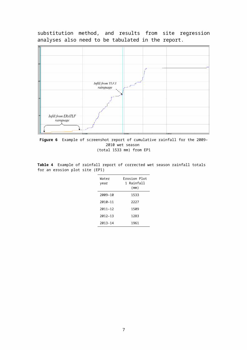
shift correctionThe method for correcting a rainfall data gap has been to apply a direct infill from one of the other erosion plot sites with reliable data (usually the site of closest proximity). However, in any given wet season period, it is first necessary to validate the accuracy of the infill by performing linear regression between actual data records from the site to be infilled with coincident records from the alternative site. These common records will be drawn from the same wet season period in which the missing data gap(s) fall. For EP sites, 10-minute rainfall totals data records coincident to both sites/times will be used to perform this analysis. Data for analysis can be easily extracted from Hydstra using HYCSV and the regression can be performed in Excel. When an R2 of > 0.95 is reached and the slope of the relationships is within 10% of 1 then the alternative data source is deemed a suitable data substitute. The data quality internal report series for each site is to report the complete and corrected rainfall dataset for each wet season period, separately. For example, the report will illustrate the cumulative rainfall hydrograph with data substitutions for each wet season (e.g. Figure 6); and a tabulation of corrected total rainfall over the complete data reporting period (e.g. Table 4). Ancillary data justifying corrections such as known data gaps, data substitution method, and results from site regression analyses also need to be tabulated in the report.

5

Figure 6 Example of screenshot report of cumulative rainfall for the 2009–2010 wet season (total 1533 mm) from EP1

Table 4 Example of rainfall report of corrected wet season rainfall totals for an erosion plot site (EP1)

Water year Erosion Plot 1 Rainfall (mm)

2009–10 1533

2010–11 2227

2011–12 1509

2012–13 1283

2013-14 1961

6

4 Shaft encoder stage trace correction Part I: general methods

This Section describes procedures for checking and correcting runoff stage trace data from the four erosion plot sites. Specific procedures to be applied include: Calibration of the stage trace to Cease-To-Flow (CTF) line; Identification of erratic or missing sensor data; and where

possible The correction of erratic or missing data by editing and/or data

substitution.

4.1 Calibration of stage trace to CTFThe CTF is the water level below which no water will flow over the weir (i.e. of the flume). The CTF values for the TLF erosion sites are defined in Saynor et al  (2013). The CTF value for each of the erosion plots is as follows: EP1 - 1.027 m EP2 - 1.000 m EP3 - 1.000 m EP4 - 1.003 m The ‘by-eye’ calibration of the primary trace to the CTF reference lines is a critical process in data cleaning and involves one or a combination of the following steps:a) A simple addition or subtraction adjustment of a series of points

associated with a discrete runoff event (or continuous series of discrete runoff events) such that points representing the beginning and/or end of each event aligned with the CTF line;

b) A value change to a single point record at either the beginning or end of an event series (usually in order of ± 1 mm), to specify when the event began, or ended; or to divide two separate events;

c) insertion of a ‘flow event division point’ between a series of events to separate a series of discrete flow events from one another (normally by inserting a point < 1mm below the CTF line);

d) inserting a point on the CTF line to define when an event began or ended

Step a) is applied first, followed by steps b) to d) when necessary. Once a trace has been calibrated to the CTF line, annotations are then added to selected stage trace points to record key stages of each individual flow event. If, after independent review, these key points require further calibration, annotations will also need to be

7

updated to reflect corrections. These stages include the time point and water level when the: a) Flume stilling basin began to fill; b) Flume stilling basin stopped filling (without flow over flume);c) Flow over the flume commenced (i.e. and is just equal to CTF

reference line value); andd) Flow over flume ends (i.e. and is just equal to CTF reference line

value). A trained technician can accurately estimate the start and end of a discrete runoff event by the shape and duration of the flow-pulse depicted by the stage trace (Figure 7). The relationship between the stage trace and the timing, magnitude and duration of rainfall also guides the technician in estimating the start and duration of runoff flow over the flume. Time-lapse photos of flow over the flume are available to validate these calibrations. Further details on these procedures have been reported in Saynor et al. (2015).

8

`Figure 7 A labelled screenshot from the Hydstra editing window showing the water level of the primary trace (variable 100.01, blue line) and a standardised series of comment

tags (italics) for two types of events (Basin fill only and runoff over flume). The Hydstra ‘©’ label indicates point records with comments entered during editing. The CTF calibration line in this example is for EP1.

1

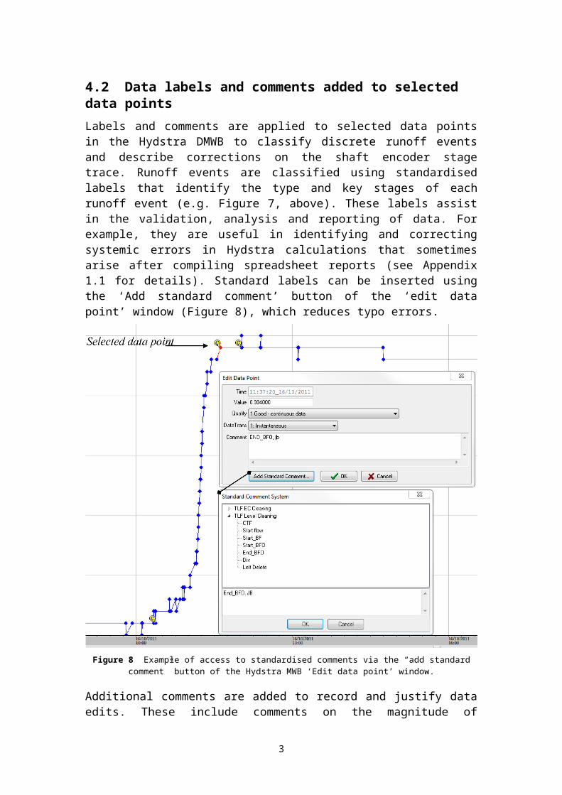
4.2 Data labels and comments added to selected data pointsLabels and comments are applied to selected data points in the Hydstra DMWB to classify discrete runoff events and describe corrections on the shaft encoder stage trace. Runoff events are classified using standardised labels that identify the type and key stages of each runoff event (e.g. Figure 7, above). These labels assist in the validation, analysis and reporting of data. For example, they are useful in identifying and correcting systemic errors in Hydstra calculations that sometimes arise after compiling spreadsheet reports (see Appendix 1.1 for details). Standard labels can be inserted using the ‘Add standard comment’ button of the ‘edit data point’ window (Figure 8), which reduces typo errors.

Figure 8 Example of access to standardised comments via the “add standard comment” button of the Hydstra MWB ‘Edit data point’ window.

Additional comments are added to record and justify data edits. These include comments on the magnitude of corrections, where and why point records were deleted, and an identifier at the beginning and end of data gaps or substitutions. Below are instances when comments should be inserted The standardised comment as described above (e.g. Figure 8)

vs. Others;

2

The correction factor applied is specified at the beginning and end of the adjustment range and will include the initials of the person applying the change (e.g. to right + 0.01, JB; to left + 0.01, JB ).

If the correction is for a single point, a comment will include the note “pt value change”;

A correction of the time at the beginning and end of events; Inserting an event division point; Photo annotations for validating start and end of flow; Inversion errors; Time synchronisation errors due to incorrect time setting; Field testing artefacts; Comments relating to events that were undertaken in the field

that could explain the data and its history (e.g. Bedload collection); and

Importantly, the initials of the person who made the comment, and the date when the comment/change is made, should be placed at the end of all comments.

4.3 Consistency checks Consistency checks of the stage trace records are undertaken to detect and correct the following types of errors: 1. Missing data ( i.e. a response in cleaned rainfall dataset but no

runoff response in shaft encoder could indicate missing runoff data);

2. Anomalous runoff events, unexplained by rainfall, should be deleted from the stage trace;

3. Time mismatches between the stage traces of different plots need to be corrected

4. Stage trace inversion due to wiring or code error;5. Incorrect multiplication factor applied to logger code when

setting up pressure transducer sensors, which can result in a mismatch between shaft encoder and pressure transducer.

Identifying missing and anomalous eventsOnce complete (for method see Section 3), the rainfall dataset provides a basis to identify true runoff events, missing data, and anomalous events in the stage trace. Time mismatchesTime mismatch errors between sites are identified and corrected by:

3

1. Notify field staff of the issue and reset the data-logger to the correct time for the problem site (time may have been set to the computer server time, set to an internet world clock);

2. Calculate the time difference in coincident rainfall responses between EP sites (Figure 9). The rainfall variable is used because it is the most time-sensitive measurement; and

3. Once the time offset is determined a time offset correction is applied to the data period (Error: Reference source not found). Because all sensors at a site will have the same timestamp, the time corrections need to be applied to all sensors attached to the logger.

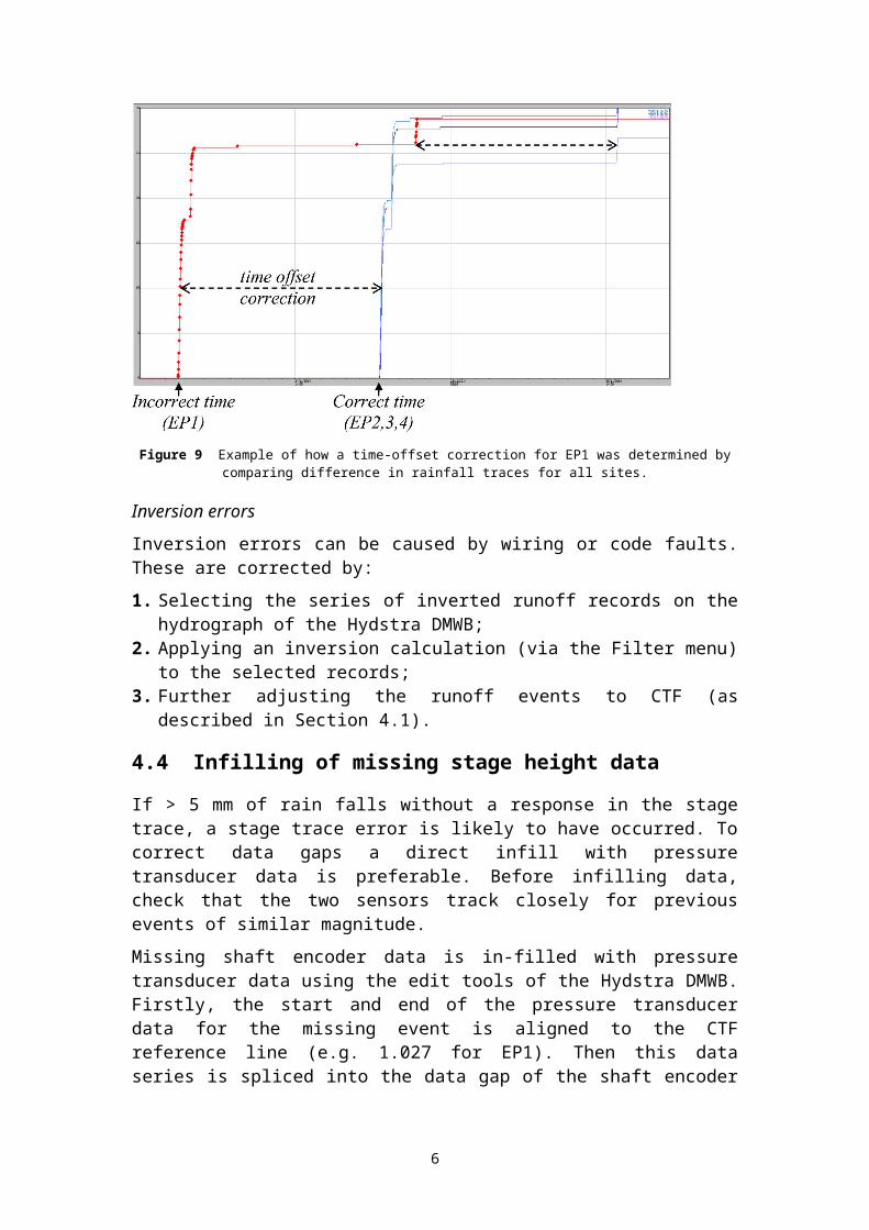
Figure 9 Example of how a time-offset correction for EP1 was determined by comparing difference in rainfall traces for all sites.

Inversion errorsInversion errors can be caused by wiring or code faults. These are corrected by:1. Selecting the series of inverted runoff records on the

hydrograph of the Hydstra DMWB; 2. Applying an inversion calculation (via the Filter menu) to the

selected records;3. Further adjusting the runoff events to CTF (as described in

Section 4.1).

4.4 Infilling of missing stage height data

If > 5 mm of rain falls without a response in the stage trace, a stage trace error is likely to have occurred. To correct data gaps a direct infill with pressure transducer data is preferable. Before infilling data, check that the two sensors track closely for previous events of similar magnitude.

4

Missing shaft encoder data is in-filled with pressure transducer data using the edit tools of the Hydstra DMWB. Firstly, the start and end of the pressure transducer data for the missing event is aligned to the CTF reference line (e.g. 1.027 for EP1). Then this data series is spliced into the data gap of the shaft encoder stage trace (100.01 M file) using the “copy reference trace” option of the Workbench edit menu. When no runoff data is recorded by either the shaft encoder or pressure transducer and rainfall and runoff has occurred, data gaps are in-filled with reliable data from the nearest site once between-site correlations are undertaken. Specific missing data periods and substitutions are tabulated in the methods and results of the Internal Report series for each erosion plot and ‘clean-data’ period (e.g. Table 5).

5

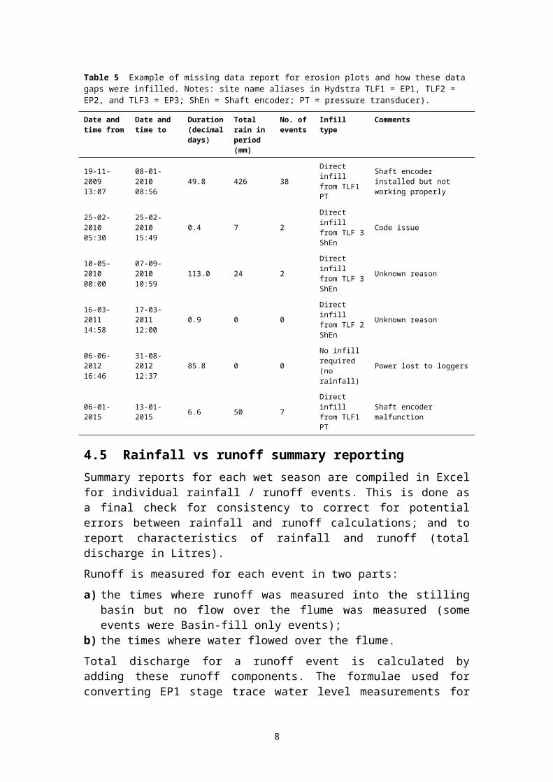
Table 5 Example of missing data report for erosion plots and how these data gaps were infilled. Notes: site name aliases in Hydstra TLF1 = EP1, TLF2 = EP2, and TLF3 = EP3; ShEn = Shaft encoder; PT = pressure transducer).

Date and time from

Date and time to

Duration (decimal days)

Total rain in period (mm)

No. of events

Infill type Comments

19-11-2009 13:07

08-01-2010 08:56 49.8 426 38

Direct infill from TLF1 PT

Shaft encoder installed but not working properly

25-02-2010 05:30

25-02-2010 15:49 0.4 7 2

Direct infill from TLF 3 ShEn

Code issue

10-05-2010 00:00

07-09-2010 10:59 113.0 24 2

Direct infill from TLF 3 ShEn

Unknown reason

16-03-2011 14:58

17-03-2011 12:00 0.9 0 0

Direct infill from TLF 2 ShEn

Unknown reason

06-06-2012 16:46

31-08-2012 12:37 85.8 0 0

No infill required (no rainfall)

Power lost to loggers

06-01-2015 13-01-2015 6.6 50 7Direct infill from TLF1 PT

Shaft encoder malfunction

4.5 Rainfall vs runoff summary reporting Summary reports for each wet season are compiled in Excel for individual rainfall / runoff events. This is done as a final check for consistency to correct for potential errors between rainfall and runoff calculations; and to report characteristics of rainfall and runoff (total discharge in Litres). Runoff is measured for each event in two parts:a) the times where runoff was measured into the stilling basin but

no flow over the flume was measured (some events were Basin-fill only events);

b) the times where water flowed over the flume.Total discharge for a runoff event is calculated by adding these runoff components. The formulae used for converting EP1 stage trace water level measurements for these two components of runoff are cited in Saynor et al. 2013.Compiling the summary involves compiling data into an Excel report template from several different Hydstra interrogation steps (outlined in Appendix 1). Also rainfall for each discrete runoff event is manually entered onto this template from viewing individual events on the Hydstra GUI. Safeguards have been inbuilt into the spreadsheet summary to check for compilation or actual database errors. If errors are encountered, corrections are applied in the Hydstra stage trace database and the spreadsheet until no further errors are detected.

6

Once corrections are completed, general statistics are then reported for each wet season and each erosion plot site in the Internal report series using the spreadsheet report template. The statistics are: Number of runoff events; Rainfall for each event; Total discharge (Litres); and The relationship between rainfall and discharge graphed for

each wet season as a scatter plot of individual runoff events.

7

5 Shaft encoder stage trace correction Part II: site-specific issues

Inspections of the plot boundaries are conducted during each wet season and early in the dry season to identify and repair structural breaches of the plot boundary as necessary.

5.1 Boundary overflow Runoff over the erosion plot containment boundary from an offsite source is referred to here as boundary overflow. Once on the plot this additional water will flow across the plot’s surface and to the outlet flume, causing an increase in the height and length (duration) of the stage trace. Hence this will cause runoff from the area of the plot containment to be overestimated by the stage trace. Data quality reports for erosion plots need to stipulate if there is a problem with boundary overflow. At the time of writing this report this was only identified as a systemic problem at EP1, and a temporary problem after a structural breach of the plot boundary in 2011 (e.g. EP2). If there is boundary overflow identified, these events need to be corrected by eye using the methods described in this section. The EP1 runon problem, its prevention, impact on data and data correction measures have been described further in Boyden and Saynor (2016). Field observations strongly suggest that, in the case of EP1, the source of excess runon was from a roadside drain adjacent to EP1 (Figure 3, above). If boundary overflow is suspected and the source of the problem is identified then physical measures to prevent the problem should be undertaken when possible. For example, in the case of EP1 the roadside drain adjacent to it was excavated to increase the volume of water that could flow through it, thereby preventing flow over the plot boundary wall. This Section describes how: 1) these problem events were identified from normal events; and 2) Corrections to remove suspected runon.

5.1.1 Comparing different site stage traces to correct for overflow Stage traces between sites are compared to identify ‘overflow’ events. For example, overflow onto EP1 was assumed to occur when, relative to EP2, there was: A delayed additional peak in the EP1 trace after rain had

stopped (e.g. Figure 10a). This pattern was typical after brief but intense rainfall events; or

A larger recessional flow (e.g. Figure 11a). This overflow pattern was typical when a large amount of rain had already fallen prior to the rain associated with the actual runoff event.

8

In the example shown in Figure 7 some 253 mm rain fell in the 48 hours prior to the end of this event

Events where overflow was indicated were corrected by hand-eye using the Draw-line mode of the Hydstra DMWB (Figure 10b and 11b). Visual cues for the corrections are provided by overlaying the original (uncorrected) stage trace for both EP1 and EP2 onto the same hydrograph datum (where zero indicated the start and cease to flow points of each event). The cumulative rainfall trace is also overlain to help determine the relationship between rainfall and runoff. Corrected runoff events were annotated at the beginning and end of each period and all changed data points were quality coded as ‘79’ - records partly estimated.

Figure 10 Evidence and correction of roadside drain overflow event where: a) overflow is indicated by a 2nd peak in the EP1 trace after a brief yet intense 31 mm rain event on the 21st December 2011; and b)

correction applied to abnormal records by manual editing (orange line).

9

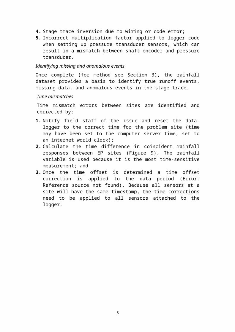
Figure 11 Evidence and correction of roadside drain overflow event where: a) overflow is indicated by the elevated EP1 stage trace in relation to EP2; and b) correction applied to abnormal records by

manual editing (orange line).

5.1.2 Estimated contribution of ‘overflow’ to runoff measured from EP1The contribution of ‘overflow’ to discharge measured from EP1 is estimated by comparing discharge measurements before and after overflow corrections are applied. Discharge should be calculated from individual events in each wet season and compiled in a spreadsheet as described in Appendix 1.2. All discharge measurements are represented graphically by water year, and presented in litres.

10

5.2 Evaluating accuracy of shaft encoder measurements at high flows Turbulence in the stilling basins has been shown to cause a disparity between the shaft encoder and pressure transducer measurements, with shaft encoder measurement underestimated (Saynor et al. 2015). For this reason the accuracy of the shaft encoder stage trace is checked against the pressure transducer for all larger runoff events. The severity of this problem appears to be greater as stilling-basin capacity decreases. It is evident at EP2, 3 and 4 in order of increasing severity problem but doesn’t seem to occur at EP1 (the site with the largest stilling basin).

Figure 12 Example of water-level disturbance in the upstream stilling basin at EP2 during the peak of a high-flow event. This turbulence is expected to cause the shaft encoder to underestimate water level.

11

6 ReferencesBos MG, Replogle JA & Clemmens AJ 1984. Flow measuring flumes

for open channel systems. Wiley, New York.

Boyden J & Saynor M 2016. Ranger Trial Landform: Hydrology – Rainfall and runoff data for Erosion Plot 1: 2009-2015. Internal Report 646, Supervising Scientist, Darwin.

Clemmens AJ, Wahl TL, Bos MG & Regplogle JA 2001. Water Measurement with Flumes and Weirs. International Institute for Land Reclamation and Improvement, Wageningen, 90-70754-55-x.

Saynor MJ, Boyden J & Erskine WD 2016 Ranger Trial Landform Hydrology – Rainfall and runoff corrections for Erosion Plot 2. Internal Report 632, Supervising Scientist, Darwin.

Saynor M, Erskine W, Moliere D & Evans K 2013. Determination of filling curves for the stilling basins, the size of the flumes and rating curves for the Rectangular Broad Crested flumes for the erosion plots on the Ranger Trial Landform. Internal report 614, January 213, Supervising Scientist Division, Darwin, Unpublished paper.

12

Appendix 1 – Data reporting methodsThis Appendix describes the reporting methods for summarising runoff over the flume for individual events. These calculations are undertaken on cleaned datasets in Hydstra then compiled and checked in Excel spreadsheets containing data processing templates. The following headings are in step sequence. The formula used to convert the stage height to discharge and total volume in litres differs for each EP site. Each formula is described in Internal report 614  (Saynor et al 2013). These conversion formulae have been set in Hydstra.

A1.1 Generating standardised comments reportsThis Appendix describes the methods used to export standardised comments report from primary runoff dataset in Hydstra (100.01); add them to the Excel spreadsheet report; and check individual runoff events for consistency.Comments can be added to individual time-point records in the Hydstra database. 1. A Comments Report is generated in the Hydstra Data Managers

Workbench as shown in the screenshot below:

Comments reports produce a time-stamped list of all comments linked to each point record value as a space-delimited text file. This function was used to extract and check standardised comments for water level (100.01, M file). These comments are summarised in an Excel spreadsheet extracted filed at the Darwin office for each water-year separately (i.e. 1/09 to the 31/08 the following year). The naming convention of these files for the 2013-2014 water year is also filed at the Darwin office.Standardised comments were checked for consistency and corrected in the Hydstra database when necessary. All Comments are added to a spreadsheet tab named “EPx_uncorrected comms” where they are sorted, filtered, and checked for time-series consistency. For example, an error point is highlighted in the time-

13

sorted list of event comments shown below (Table A1.1). That is, the “Start flow” comment must be followed by a CTF comment to be correct).

14

Table A1.1 Time-sorted list of uncorrected comments with an inconsistency in the logical sequence of comments highlighted

Plot File Variable Date / time Value Comment

EP1 .M 100.01 04-11-2014 17:36:50 0.794 Start_BFO

EP1 .M 100.01 04-11-2014 17:57:40 0.855 END_BFO

EP1 .M 100.01 04-11-2014 18:05:00 0.856 Start_BF

EP1 .M 100.01 04-11-2014 18:10:38 1.027 Start flow

EP1 .M 100.01 04-11-2014 19:27:50 1.027 CTF

EP1 .M 100.01 06-11-2014 20:15:30 1.027 Start flow

EP1 .M 100.01 11-11-2014 15:28:00 0.96 Start_BFO

EP1 .M 100.01 11-11-2014 15:37:50 0.974 END_BFO

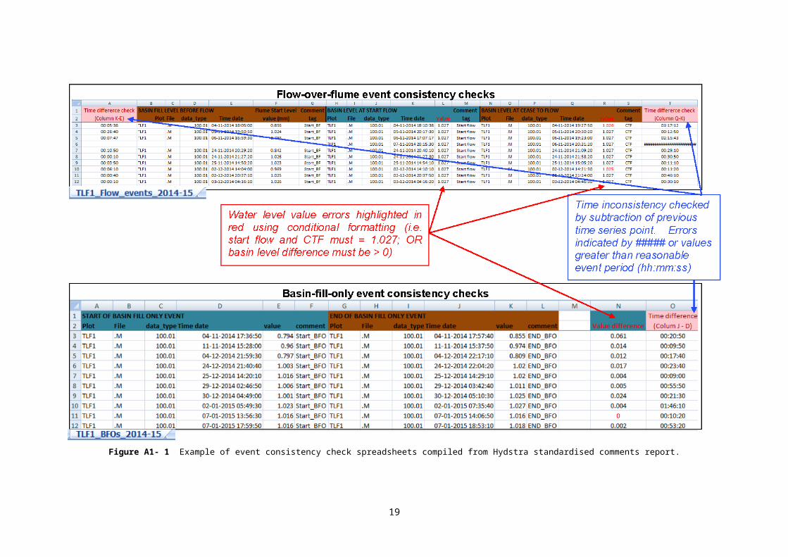
A1.2 Summarise discharge for individual events using a standardised spreadsheet templateCorrected events are summarised in two spreadsheets tables, one for Flow-over-flume-events (with prefix name EP1_Flow_events_) and the other for Basin-fill-only events (with prefix name (TLF_BFOs_). Time sequence and water-level values are checked for consistency with further corrections made, when necessary, in the Hydstra database. For example in Figure A1.1, time-series errors for individual events compiled by the different methods were identified using the ‘time difference’ checks in columns A and T. Column ‘A’ compared differences between CTF recorded in Hydstra comments against the CTF calculated using the HYEXTREME report filter. In this case two types of error were identified. If a CTF comment tag was missing in Hydstra, this would result in time errors from the spreadsheet row (time point) onwards from where that error occurred (i.e. adding a CTF comment tag to Hydstra at the appropriate point would prevent this error occurring again). A time error would also be flagged when additional data points occurred on the CTF line and adjacent of the actual (commented) CTF point on the stage trace. Deleting the no-data points from the CTF line would remove this error.

15

Figure A1- 1 Example of event consistency check spreadsheets compiled from Hydstra standardised comments report.

16

Runoff volume for each discrete ‘flow over flume’ event is calculated by 1) converting EP1 stage height to cumulative discharge using HYCRSUM with conversion parameters specified in Saynor et al. 2013; then 2) extracting these data at 1-minute intervals using HYCSV and applying them to programmed Excel spreadsheet to produce a total discharge summary for each discrete event.

A1.2.1 Run HYCRSUM to convert stage height (100.01) to total volume (153.01) in Litres. Note this conversion process goes initially to discharge rate in m3/sec (Hydstra variable code 140) and then to cumulative discharge volume in litres over time (Hydstra variable code 153). It is also dependent upon the correct conversion formulae being loaded in the Hydstra conversion tables. Open HYEXPLORE and type “ HYCRSUM” at the bottom of the screen and click on “Run”

17

1. In HYCRSUM click on Program menu to open a drop down box and select Jobs. Note steps 2 to 4 can sometimes be bypassed if the job parameters have already been loaded for the last previous job run, in which case F8 will automatically load these details.

2. From the list of HYCRSUM Parameter Jobs select “Discharge -> volume (L)”

18

19

3. “Load Job” will be highlighted – Click on it

4. Input the Primary Input File for HYCRSUM populate the following parameters for TLF1 (= EP1). Note if these parameters have been loaded on a previous job type F8 to reload these parameters

5. Check that the Output File extension (U) is not being used then

Run HYCRSUM. Note when start default and end time are the

20

same the dataset will be produced for the entire time-series of the input.

6. Check the output file for errors. If correct add to preliminary Hydstra archive (M files)

A1.2.2 Calculate runoff volume for discrete events over one wet season1. Use HYCSV to extract cumulative runoff in litres at 1-minute

intervals for a particular wet season period.

2. The output CSV file will automatically open in Excel (by specifying “X” as the output file type). An example of the output format is provided below:

21

3. Create a new spreadsheet template from the completed “Litres over Flume” individual events files in SPIRE (a hyperlink to completed examples is filed at the Darwin office;

4. Paste the data into the appropriate columns of a prepared “Litres over Flume” spreadsheet, an example of which is filed at the Darwin office. Be careful not to overwrite areas of the spreadsheet containing embedded formulae. Also ensure that the embedded formulae (columns C to D) are copied across the input data rows range;

22

5. Copy the entire data and formulae calculation range, open a blank worksheet, right click in the top left corner of the sheet and select Paste Special from the dropdown menu.

6. From the Paste Special window select Values then OK

7. Select the entire data block from the header row and then sort it by column D (time) and calculate total runoff per discrete event (column F)

23

8. Open a “Total runoff” spreadsheet template for the particular wet season (copy from previous wet seasons and remove input data) and open the “Working sheet” tab then scroll across to Columns M and N (the section for “Litres over flume” )

9. Go to the “Litres over Flume” spreadsheet and copy the sorted all discrete events from columns D (i.e. Step 7 above from row 6 to end of discrete events)

10. In the “Total Runoff” spreadsheet select the first row of column M under the header “End of flow event” , right click, paste special, paste as values.

11. Repeat steps 9 and 10 for Column D data from the “Litres over Flume” spreadsheet (Step 7), but paste these data into Column N of the “Total Runoff” spreadsheet.

24

12. Check that the row time-sequence of data taken from the Litres over flume spreadsheet align correctly with data compiled from other sources on spreadsheet. To do this, view values in column L (calculated time difference). Time sequence error are indicated if values are ≥ 1 minute or a “#####” value is returned.

25

A1.3 Apply HYEXTREM to check number of discrete events in spreadsheet summary 1. Open HYEXTREM from HYEXPLORE and populate the

parameters to the following specifications for a particular wet season period. These settings will detect all events that exceed or equal the CTF line (1.027 for TLF1)

2. Select the columns B and C (header is ‘start’ and ‘end’) of the output spreadsheet

3. Right click on the selected columns and reformat the columns to “dd/mm/yyyy h:mm” using the number format tab (Custom)

26

4. Replace all “_” characters in columns B and C with a space (Use search and replace all)

5. Now sort the HYEXTREM output on the column F header (Extreme). Then delete all rows with the CTF value.

6. Now resort the remaining rows by increasing time/date in column B header (start)

7. Select and copy all data rows (excluding the header) from the output and paste them into the appropriate section (columns E to J) and time-sequence row of the “Total runoff” summary spreadsheet

27