IPUMS User Note: Issues Concerning the Calculation of Standard Errors (i.e.,

variance estimation)Using IPUMS Data Products

by Michael Davern and Jeremy Strief

Producing accurate standard errors is essential for both the scholarly research and official

policy uses of the data because they indicate the precision of the estimates and the

statistical significance of hypothesis tests (e.g., whether estimates of poverty differ from

one year to next, or whether one state has a higher poverty rate than another). Statistical

significance provides the standard of evidence for statistical arguments, and the errors

allow us to gauge our level of uncertainty associated with specific estimates. In theory,

standard errors are relatively easy to compute if samples have been collected using

simple random sampling. However, survey data is often based on a complex, multistage

sample design whose information needs to be accounted for when calculating standard

errors. Failure to account for the stratification, clustering, and weighting used in the

survey sample design generally results in serious underestimation of standard errors

(Kish 1992, 1995; Lohr 2000).

Sample Design, Standard Errors and the Survey Data

There are three important elements that determine the effect of the complex survey

sample design on standard errors: clustering, stratification, and weighting. Cluster

sampling involves the grouping of the population into convenient aggregations of

1

observations, such as people in households, households in blocks, and blocks in counties.

The sampled units are drawn from some of these clusters at the exclusion of others (Kish

1995). Stratification is also a grouping of elements, or clusters, but in this case elements

or clusters are drawn from each stratum (that is, all strata are included in the sample),

sometimes at different sampling rates (Kish 1995). For example, in a given strata one in

2,000 households is sampled, whereas in others one in 1,000 households is sampled.

Finally, weighting is a technique for adjusting sample data to correct for design features

such as oversampling and design deficiencies such as nonresponse. Base probability

weights are the inverse probability of being selected into the sample. For example, if a

person has a one in 1,000 probability of selection, the weight is 1,000. Weights can

increase the variance of estimates when some population elements have a higher weight

than others (Kish 1992). The ratio of an estimated sampling variance that takes these

components into account to an estimated sampling variance that ignores clustering,

weighting, and stratification is called the design effect (Kish 1995). In most cases, the

standard errors calculated that take clustering, stratification, and weighting into account

are larger than those that do not; the design effect therefore is usually greater than 1 for

complex sample surveys.2

The effect of clustering is driven by the intraclass correlation coefficient ρ—

which expresses the correlation between members of a sampled cluster (e.g., household),

or the percentage of the total variance found between clusters—and by the size of the

cluster (Kish 1995). The design effect due to clustering is determined by:

2

1+ρ(b-1). (1)

Here ρ is the intraclass correlation and b is the size of the cluster. In cases where the

intraclass correlation is 0 the design effect due to clustering is simply 1. However, when

the intraclass correlation coefficient is greater than 0 the design effect due to clustering

will be greater than 1.

When using information from a survey data set that includes clustered

observations, the intraclass correlation coefficient will vary across statistics. For

example, households function as clusters in the CPS ASEC. When developing estimates

for concepts that are highly correlated within a household, such as whether a person is in

poverty or covered by health insurance, the intraclass correlation will be larger. For other

concepts like personal income, the intraclass correlation coefficient may be lower –

knowing the income of one person in the household does not provide reliable information

about the earnings of other people in the household. On the other hand, knowing whether

one person in the household is in poverty is highly related to whether another person in

the same household is also in poverty, since entire families are assigned the same poverty

status.

The design effect can be decreased under some forms of stratification (Kish 1992,

1995). Stratification can reduce the design effect when the elements or clusters within a

stratum tend to be homogeneous (in contrast to the effect of clustering where

homogeneity within clusters leads to a larger design effect). For example, if one stratum

within a study has a group of households that are all very likely to be in poverty and

3

another has households not likely to be in poverty, the design effect for poverty estimates

will be reduced when stratification is taken into account in variance estimation.

Weights have components adjusting for differential probabilities of selection,

nonresponse, and sample noncoverage (e.g., when the sample frame does not perfectly

cover the population of interest). To the extent that the weights are heterogeneous, the

size of the design effect can increase. Weights become heterogeneous in surveys because

some elements have higher probabilities of selection than others (by design or by

circumstances dictated by the sample frame), because some groups have higher response

propensity than others, or because some subgroups are under-represented by chance

relative to known external population distributions (Kish 1992). Kish gives the simple

formulation of 1+L (the “L” stands for “Loss” of sample efficiency) to approximate the

effect of the sample weights on the design effect. In general, the more heterogeneity in

the weights, the higher the design effect will be.

1+L=(nΣk2j)/(Σkj)2. (2)

Here n is the unweighted sample size, and k is the survey weight for the jth person. In

effect, the equation is the unweighted sample size multiplied by the sum of the squared

weights. This total then is divided by the sum of the weights squared. The result is an

approximation effect on sampling variance due to heterogeneity among weights.

Overall, weighting and clustering tend to increase the design effect and

stratification tends to decrease it. In complex sample surveys, however, the impacts of

4

clustering and weighting tend to be larger than those of stratification, so the design effect

is greater than 1.

Methods of Standard Error Estimation

Seven methods of standard error estimation are: 1) the basic “simple random

sample” approach which assumes that every sampled person is drawn independently and

completely at random; 2) the Census Bureau’s “design factor” (called generalized

variance parameters in the Current Population Survey) approach, which is produced and

used by the Census Bureau (U.S. Census Bureau 2001, 2002a); 3) the “robust variance”

estimation approach (also known as the sandwich estimator, or the Huber-White

estimator); 4) a “survey design-based estimator,” which uses both an identified stratum

and a clustering variable; 5) “random group methods,” which examine variability

between subsamples; 6) “replicate methods,” which provide multiple sets of perturbed

sampling weights; and 7) the “Polya Posterior method,” which constitutes a Bayesian

approach to survey analysis.

Simple Random Sample

We use two equations to estimate the “simple random sample” standard errors.

Expression (3) is used for rates and expression (4) is used for averages. The assumption

that each element was selected as part of a simple random sample should, in general,

produce smaller standard errors than any other method considered in this paper. Standard

errors based upon simple random sampling do not take into account the clustering of

5

people within sampled households, nor the clustering of households within USUs or

PSUs for example. Because observations within clusters are often correlated, clustering

tends to inflate standard errors. However, simple random sample standard errors need

not always be smallest. In some instances, it is possible for the design-adjusted standard

error to be smaller than the simple random sample standard error when the effect of

stratification is more pronounced (Kish 1995).

For a binomial variable (e.g., poverty versus not in poverty), equation (3) yields

the simple random sample standard error:

nPP /)100(1 −=σ , (3)

where P is the weighted rate of insurance coverage or poverty and the n is the total

number of people included in the sample used to calculate the statistic of interest. Note

that equation (3) ignores the finite population correction of (1-Q), where Q is the

proportion of units in the population which were sampled. When Q is relatively small (as

is the case with most IPUMS datasets), the finite population correction becomes

negligible.

For the continuous variables like income, the standard error is computed using

Formula 4. As was the case with the binomial standard error, formula (4) ignores the

finite population correction:

)1(/2 −= nS xσ , (4)

6

where Sx is the standard deviation of the continuous variable in question, and n is the total

number of people over age 15 in the state that were included in the sample.

Design Factor Approach (i.e., Generalized Variance Approach)

When the Census Bureau produced the first public use microdata samples, computing

resources were scarce and statistical software was rudimentary and the Census Bureau

could not release all the sample design information used to select the samples in order to

protect respondent confidentiality and privacy. It was therefore impractical for

researchers to calculate standard error estimates that accounted for the complex design of

the samples. Therefore, the Census Bureau calculated “design factors” (originally termed

“standard error adjustment factors” and called “generalized variance parameters in the

Current Population Survey documentation) for specific variables, and researchers were

advised to multiply their conventional standard errors by the adjustment factor to account

for the complex sample design (US Census Bureau 2003). The original IPUMS project

developed comparable adjustment factors for the earlier census years.

The strategy of using design factors to correct for complex sample designs has several

serious weaknesses and we do not recommend their use with IPUMS data:

• The design factors published by the Census Bureau are not always accurate; adjusting for the actual sample design used to select cases, we have found errors in the published design factors ranging as high as 200 percent in the Current Population Survey (Davern et al. 2006; 2007).

• The needed adjustments are not uniform across categories of the same variable. To give just one example, the true design factors for the “Head” and “Spouse” categories

7

of the household relationship variable are always much lower than the design factors for “Child” or “Boarder,” since the effects of clustering are much more pronounced for the latter categories. The Census Bureau, however, publishes only one design factor for this variable, representing the average of all the categories.

• The design factors are not suitable for multivariate analyses. The Census Bureau documentation for the 1980 microdata sample recommended that when adjusting the standard errors of a crosstabulation, users should simply choose the largest adjustment factor, but there is no theoretical or empirical justification for this approach (U.S. Census Bureau 1982).

The great majority of IPUMS-based research involves complex regression models that

control for many covariates (http://www.ipums.org/usa/research.php). The Census

Bureau’s design factors are inappropriate for the exploration of associations among

variables and are especially problematic when performing complex analyses. It would be

impossible for the decennial census technical documentation to provide guidance for all

possible types of analyses and dependent variables. Thus, researchers need to be able to

produce standard errors tailored to their particular analyses and we do not recommend the

use of design factors when working with IPUMS data as better alternatives are available.

Robust Variance

The “robust variance” estimation approach – also known as the sandwich estimator, the

Huber-White estimator (SAS 1999), or the “first-order Taylor series linearization”

method – is implemented using SAS version 8.2. Specifically, we use the “surveymean”

procedure with states designated as subpopulations. In using these survey procedures, we

declare only the survey weights among the survey features, which invokes the robust

standard error estimator. Although the robust standard error estimator does not explicitly

control for any of the clustering features of survey data per se in generating standard

8

errors, we include it as one of our four standard error estimators. This is because it is

common in the research literature to read that standard errors are calculated using

STATA (2001), SPSS (2003), or SAS (1999) survey adjustment procedures, but no

mention is made of clustering or strata adjustments. If the procedures are used by

themselves, without a cluster or strata adjustment, then the robust standard error is the

resulting estimator.

Survey Design-Based Estimator

The “survey design-based” estimator takes account of the probability weight, clustering,

and stratification of the survey in estimating the standard errors. For our analysis, we use

the survey estimator implemented in SAS version 8.2. Like the robust estimation

method, the survey design-based method uses a Taylor Series estimation approach. But

unlike the robust estimation technique, this method explicitly controls for both

stratification and clustering. In this study, we use a Taylor Series survey design-based

estimator to compute the variances identifying the highest (i.e., first) level of clustering

(Hansen, Hurwitz, and Madow 1953; Woodruff 1971; Kalton 1977; Rust 1985). Even

though this “ultimate cluster” approach to estimating the design effect is based on the

sample’s first stage of clustering, it does include, in expectation, any subsequent stages of

variability as well.8

Random Group Methods Random group methods argue that variability associated with the original sampling

design can be estimated by the variability between subsamples. For example, a survey

9

with 10,000 units might be divided into 100 subsamples of size 100. Each unit from the

full dataset is randomly assigned to exactly one subsample.

General forms of subsample variance estimators are given in equations (7) and (8). For

both equations, R represents the number of subsamples into which the original sample is

divided;μ is the population parameter of interest, μ is the estimate ofμ from the full

sample, and rμ is the estimate ofμ using only data from the rth subsample. In general, the

subsample estimate rμ will have the same algebraic form as μ . Equation (7) examines

the variability of the rμ ’s about their mean, ∑=

=R

r

r

R1

ˆˆ μμ . Equation (8) examines the

variability of the rμ ’s about the full sample estimate μ . Either estimator is reasonable,

although equation (8) will generally yield more conservative (i.e. larger) variance

estimates (Wolter 1985).

∑=

−−

=R

rrRR

SE1

2)ˆˆ()1(

1)ˆ( μμμ (7)

∑=

−−

=R

rrRR

SE1

2)ˆˆ()1(

1)ˆ( μμμ (8)

The process by which the subsamples are drawn should mirror the original survey design.

In a complex multistage survey, the subsamples would ideally utilize design information

10

like weights, clustering, and stratification. However, such information is not available in

many IPUMS datasets, such the ACS files. Even if not all the design information is

available, subsamples should be constructed according to whatever design information is

made public.

Replicate Methods

Replicate methods argues that a sample can be conceived as a miniature version of the

population. Instead of taking multiple samples from the population to construct a

variance estimator, one may simply resample the full, original sample. The exact

meaning of “resample” depends on the particular method employed.

A whole host of methods fall under the category of replication. Balanced repeated

replication, the jackknife, and the bootstrap are three popular methods (Lohr 1999). In

the 2005 ACS, the Census Bureau implements a replicate technique known as successive

difference replication (Fay and Train 1995). The basic idea is to perturb the sampling

weights in a balanced way and then to calculate new estimates based on each set of

perturbations. The variability between the set of new estimates may be used as a variance

estimate for the original quantity of interest.

Successive difference replication may be executed in the 2005 ACS data, as the user has

access to 80 sets of perturbed weights. For each of these 80 sets, the user will estimate

11

the quantity of interest in the usual way. Then a variance estimate may be calculated

with equation (9).

∑=

−=80

1

2)ˆˆ(804)ˆ(

rrSE μμμ (9)

In equation (9),μ is the population parameter of interest, μ is the estimate ofμ from the

full sample, and rμ is the estimate ofμ using the rth set of perturbed weights. The

presence of the number “4” in equation (9) may seem mysterious, since most standard

error formulas take the simple average of each squared deviation from the mean.

Equation (9) differs from most standard error formulas due to the unique mathematical

properties of successive difference replication (Fay and Train 1995).

The perturbed weights are produced internally by the Census Bureau, so the weights

reflect all the relevant design information. Therefore replicate weights in IPUMS may

yield better variance estimates than the subsample weights, which are produced without

full knowledge of the design.

Bayesian Methods

The hallmark of Bayesian methodology is the assumption of a mathematical model that

relates the sampled units to the unsampled units. Design information is not directly used

in the computation of Bayesian estimates, except when such design information is

thought to inform the relationship between sampled and unsampled units. One type of

Bayesian methodology is based upon the Polya Posterior (Ghosh and Meeden 1997). The

12

general idea is to simulate—using both prior information about the population and

information gleaned from the sample—complete copies of the population. Variability

between these copies may be used as a variance estimate for any quantity of interest.

The only program which currently can invoke the Polya Posterior is found within a

freeware statistics program called R (http://cran.r-project.org). The “polyapost” package

within R contains the specific commands needed to perform Bayesian variance

estimation, and this package can be downloaded from

http://cran.r-project.org/src/contrib/Descriptions/polyapost.html. Detailed instructions for

using the “polyapost” package can also be downloaded from the above webpage.

In order for Bayesian variance estimates to perform well, survey design information is

needed only insofar as it informs the relationship between the sampled and the unsampled

units. If one has reason to believe that the sample is representative of the population,

then no survey design information is necessary. However, due to the complexity of the

Census Bureau survey designs, there is good reason to believe that many IPUMS samples

are not exactly representative of the population at large. For instance, in those surveys

where the Census Bureau oversampled African Americans or other minority groups,

Bayesian variance estimation would require that one know the degree to which the

sample over-represents those minority groups. The exact sampling design is irrelevant,

just so long as one knows the degree of over-representation. Such information would be

13

formally expressed in a mean constraint: if the true proportion of African Americans in

the population is 15%, then the relevant mean constraint is

∑=

=n

iii wa

1.15.0 (10)

Equation 10 assumes a sample of size n, and it lets wi be the proportion of units in the

population represented by person i. Furthermore, ai is an indicator variable which equals

1 if person i is African-American and equals 0 otherwise. Specific instructions for

implementing such a constraint in R can be found at

http://cran.r-project.org/src/contrib/Descriptions/polyapost.html.

Given the large sample size and complexity of IPUMS data, Bayesian methods may not

yet be practical to implement. The “polyapost” package operates most efficiently on a

PC with sample sizes less than 100, whereas many researchers may be studying IPUMS

datasets having sample sizes in the thousands or millions. Research is currently

underway to simplify Bayesian methodology and make it more practical for IPUMS

users.

Warning about Case Selection Using the IPUMS Data: The Issue of Domain

Estimation

Often it is of interest to estimate facts about a subset of the full population, rather than the

full population itself. For example, the full population for the 2005 ACS includes all

United States residents not living in group quarters, but a researcher might utilize the

14

ACS to study the subpopulation of African American males or American women earning

a yearly salary greater than $80,000. When such subpopulations are being studied,

statistical estimation procedures fall under the category of domain estimation, and

subpopulations are called domains.

Because the total size of the subpopulation is unknown, it is more complicated to

estimate the standard error of a domain mean than a full population mean. Simply

restricting the dataset to the subpopulation of interest and then invoking a standard error

formula is not correct, even if weights are properly included in the analysis. This is due

to the fact that some clusters may contain no observations from the domain of interest;

ignoring such clusters generally yields an underestimate of the standard error (Lohr

1999).

To properly estimate means and standard errors within a domain, one should utilize the

built-in domain estimation features of statistical packages. For all mainstream packages,

it is important to not create a new dataset which only includes the domain of interest.

Rather, one should apply domain estimation procedures to the full dataset. In SAS, one

would invoke a domain statement within proc surveymeans; in Stata, one would use the

subpopulation command.

Although each statistical package requires different coding to invoke domain estimation,

all packages perform roughly equivalent statistical operations. If dy is the true mean of

15

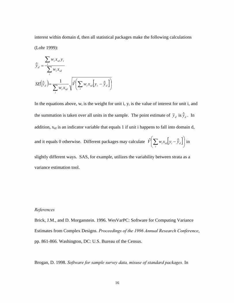
interest within domain d, then all statistical packages make the following calculations

(Lohr 1999):

( ) [ ]⎟⎠

⎞⎜⎝

⎛−=

=

∑∑

∑∑

idiidi

iidi

d

iidi

iiidi

d

yyxwVxw

ySE

xw

yxwy

ˆˆ1ˆ

ˆ

In the equations above, wi is the weight for unit i, yi is the value of interest for unit i, and

the summation is taken over all units in the sample. The point estimate of dy is dy . In

addition, xid is an indicator variable that equals 1 if unit i happens to fall into domain d,

and it equals 0 otherwise. Different packages may calculate [ ]⎟⎠

⎞⎜⎝

⎛−∑

idiidi yyxwV ˆˆ in

slightly different ways. SAS, for example, utilizes the variability between strata as a

variance estimation tool.

References

Brick, J.M., and D. Morganstein. 1996. WesVarPC: Software for Computing Variance

Estimates from Complex Designs. Proceedings of the 1996 Annual Research Conference,

pp. 861-866. Washington, DC: U.S. Bureau of the Census.

Brogan, D. 1998. Software for sample survey data, misuse of standard packages. In

16

Encyclopedia of Biostatistics, Volume 5 (P. Armitage and T. Colton, eds.). New York:

Wiley, pp. 4167-4174.

Davern, M., L.A. Blewett, B. Bershadsky, K.T. Call, and T. Rockwood. 2003. “State

Variation in SCHIP Allocations: How Much Is There, What Are Its Sources, and Can It

Be Reduced.” Inquiry 40(2): 184-197.

Davern, M., T. Beebe, L.A. Blewett, K.T. Call. 2003. "Recent Changes to the Current

Population Survey: Sample Expansion, Health Insurance Verification and State Health

Insurance Coverage Estimates." Public Opinion Quarterly 67(4):603-26.

DeNavas-Walt, C. and R. Cleveland. 2002. Money Income in the United States: 2001.

Washington DC: US Census Bureau.

Dippo, C.S. and K.M. Wolter. 1984. “A Comparison of Variance Estimators Using the

Taylor Series Approximation.” ASA Proceedings of the Section on Survey Research

Methods, pp. 112-121. Arlington, VA: American Statistical Association.

Glied, S., D.K. Remler, and J.G. Zivin. 2002. “Inside the Sausage

Factory: Improving Estimates of the Effects of Health Insurance Expansion Proposals.”

Milbank Quarterly 80(4):603-636.

17

Hammer, H, H. Shin, and L. Porcellini. 2003. “A Comparison of Taylor Series and JK1

Resampling Methods for Variance Estimation.” Hawaii International Conference on

Statistics and Related Fields. Honolulu Hawaii. June 5th-8th, 2003.

Hansen, M.H., W. Hurwitz, and W. Madow. Sample Survey Methods and Theory. 1953.

New York: Wiley and Sons.

Health and Human Services Inspector General. 2004. “SCHIP: States’ Progress in

Reducing the Number of Uninsured Kids.” Office of the Inspector General, Health and

Human Services. Washington DC. http://www.oig.hhs.gov/oei/reports/oei-05-03-

00280.pdf

Kalton, G. 1977. Practical methods for estimating survey sampling errors. Bulletin of

the International Statistical Institute 47(3):495-514.

Kish, L. 1992. Weighting for Unequal Pi. Journal of Official Statistics 8(2):183-200.

Kish, L. 1995. Survey Sampling, Wiley Classics Library Edition. New York: Wiley and

Sons.

Kish L. and M.R. Frankel. 1974. Inference from Complex Samples. Journal of the Royal

Statistical Society B (36):1-37.

18

Krewski, D. and J.N.K. Rao. 1981. Inference from stratified samples: Properties of

Linearization, Jackknife and Balanced Repeated Replication Methods. Annals of

Statistics 9:1010-1019.

Lepkowski, J.M. and J. Bowles, 1996. Sampling error software for personal computers.

Survey Statistician 35:10-17.

Lohr, S. 2000. Sampling: Design and Analysis. Pacific Grove, CA: Duxbury Press.

Mills, R. 2002. Health Insurance Coverage in the United States for 2001. Washington,

DC: US Census Bureau.

National Center for Health Statistics. 2000. “Design and Estimation for the National

Health Interview Survey, 1995-2004.” Vital and Health Statistics Series 2 (130): 1-41.

Proctor, B. and J. Dalaker. 2002. Poverty in the United States: 2001. Washington DC:

US Census Bureau.

Rust, K. 1985. Variance estimation for complex estimators in sample surveys. Journal

of Official Statistics 1(4):381-397.

19

SAS. 1999. Documentation for SAS Version 8. Cary, NC: SAS Institute, Inc.

SPSS. 2003. Correctly and Easily Compute Statistics for Complex Sampling. Chicago,

Illinois: SPSS Inc. http://www.spss.com/complex_samples/

STATA. 2001. Reference Manual. College Station Texas: STATA Press.

US Census Bureau. 2001. Source and Accuracy of the Data For the March 2001 Current

Population Survey Microdata File. Washington, DC: US Census Bureau.

US Census Bureau. 2002a. Source and Accuracy of the Data For the March 2002

Current Population Survey Microdata File. Washington, DC: US Census Bureau.

US Census Bureau. 2002b. Current Population Survey: Design and Methodology.

Technical Paper #63RV. Washington, DC: US Census Bureau.

Weng, S.S., F. Zhang, and M.P. Cohen. 1995. Variance Estimates Comparison by

Statistical Software. ASA Proceedings of the Section on Survey Research Methods, pp.

333-338. Arlington, VA: American Statistical Association.

Woodruff, R.S. 1971. A Simple Method for Approximating the Variance of a

Complicated Estimate. Journal of the American Statistical Association 66(334)411-14.

20

Davern, Michael, Arthur Jones Jr., James Lepkowski, Gestur Davidson, and Lynn A. Blewett. “Estimating Standard Errors for Regression Coefficients Using the Current Population Survey’s Public Use File.” Forthcoming Fall 2007. Inquiry.

Davern, Michael, Arthur Jones Jr., James Lepkowski, Gestur Davidson, and Lynn A. Blewett. 2006. “Unstable Inferences? An Examination of Complex Survey Sample Design Adjustments Using the Current Population Survey for Health Services Research.” Inquiry. 43(3): 283-97.

Fay, R.E. and Train, G.F. “Aspects of survey and model-based postcensal estimation of

income and poverty characteristics for states and counties.” Proceedings of the ASA,

1995.

Ghosh, M. and Meeden, G.D. Bayesian Methods for Finite Population Sampling. New

York: Chapman & Hall, 1997.

Lohr, S.L. Sampling: Design and Analysis. New York: Duxbury Press, 1999.

Wolter, K.M. Introduction to Variance Estimation. New York: Springer Verlag, 1985.

21