IPTC 17670-MS

An Accurate Volumetric Calculation Method for Estimating Original Hydrocarbons in Place for Oil and Gas Shales including adsorbed Gas using High-Resolution Geological Model Jérémie Bruyelle, Terra 3E Dominique R. Guérillot, Terra 3E (now with Qatar Petroleum Research & Technology Center)

Copyright 2014, International Petroleum Technology Conference This paper was prepared for presentation at the International Petroleum Technology Conference held in Doha, Qatar, 20–22 January 2014. This paper was selected for presentation by an IPTC Programme Committee following review of information contained in an abstract submitted by the author(s). Contents of the paper, as presented, have not been reviewed by the International Petroleum Technology Conference and are subject to correction by the author(s). The material, as presented, does not necessarily reflect any position of the International Petroleum Technology Conference, its officers, or members. Papers presented at IPTC are subject to publication review by Sponsor Society Committees of IPTC. Electronic reproduction, distribution, or storage of any part of this paper for commercial purposes without the written consent of the International Petroleum Technology Conference is prohibited. Permission to reproduce in print is restricted to an abstract of not more than 300 words; illustrations may not be copied. The abstract must contain conspicuous acknowledgment of where and by whom the paper was presented. Write Librarian, IPTC, P.O. Box 833836, Richardson, TX 75083-3836, U.S.A., fax +1-972-952-9435

Abstract The emergence of liquid-rich and gas shale reservoirs presents major strategic opportunities and challenges for the oil and gas industry. Accurate estimation of Stock Tank Oil and Gas Initially In Place (STOIIP & GIIP) is one of the priority tasks before defining the reserves. An accurate method is proposed to calculate hydrocarbon volumes using high-resolution geological models taking advantage of huge improvements made during last decade in the field of characterization and geological modeling of unconventional reservoirs. This exact method provides fluids in place in reservoir and surface conditions with an extended black-oil formulation including condensates. The physic including the equilibrium between gravity and eventually capillary forces and adsorbed gas is fully respected using, for each lithofacies, the most accurate available geological description with 3D porosity distributions, Langmuir isotherms (Langmuir, 1918), capillary pressure curves, and thermodynamic data. Adsorbed and liquid-rich gases are considered. This method calculating hydrocarbons in place is the natural endpoint of any workflow devoted to the geological modeling of newly discovered reservoirs, particularly suited to heterogeneous reservoirs. The knowledge generated by this calculation has significant impact on fracturation programs to increase the recovery rate and field development planning. Introduction The characterization of volume of fluids in place in shale reservoir is a challenging task for many reasons, in particular because of the adsorbed gas which is a way of trapping gases in geological formations. The adsorption capacity of a gas on a rock depends on many parameters such as temperature, pressure, gas type and rock type. Shale gas is generated in source rocks, which are usually made of clay with high organic matter content. However, the organic content depends on the maturity of the organic matter from which they come from. Also, the maturity of the organic matter itself depends on the temperature history during the reservoir formation. Thus, in the same sedimentary basin, conventional reservoir can be formed from hydrocarbon expelled of unconventional reservoir. This is the case in the United States, where sedimentary basins that produce large quantities of unconventional hydrocarbons were already conventional oil and gas basins exploited for their conventional hydrocarbons. As for conventional reservoirs, there are large uncertainties on many parameters of the geological model. For shale reservoirs, another source of uncertainty is being added due to specific parameters related to them. Shale makes a wide variety of highly differing formations. All these formations differ from conventional reservoirs, and shale rock characteristics can differ from shale to shale, and even within the same shale. This paper presents an efficient volumetric calculation method to facilitate the evaluation of original hydrocarbons in place for oil and gas shales including adsorbed gas. The proposed method does not estimate the fluids in place using stochastic simulation methods to distribute spatially the saturations of the fluid phases, but it calculates them rigorously using the right

2 IPTC 17670-MS

physics of the phenomena. A high-resolution geological model is used to maintain the best accuracy and not losing resolution due to upscaling. For each cell of the geological model, an exact volume calculation is performed, i.e. respecting all physics phenomena involved: equilibrium of gravity forces and capillary forces and quantification of the adsorbed gases. An application of this accurate calculation is explained below detailing first the requested data and then explaining how are calculated Stock Tank Oil Initially In Place (STOIIP) and Gas Initially In Place (GIIP), and demonstrated on a synthetic case study including different qualities of shales. Uncertainties on geological parameters (including Langmuir parameters) are propagated to deliver the associated uncertainties on these volumetric calculations which are finally given in surface and reservoir conditions. Note that saturation and pressure of all phases are also given as a byproduct of the approach. Requested Data The objective of the proposed calculation method is to provide a detailed assessment of the volumes of fluids in place. Hydrocarbon volumes depend upon three types of parameters: rock properties, fluids properties and rock-fluid interactions. The necessary data are:

1) A high resolution geological model, 2) The thermodynamic data and 3) Capillary pressure curves and adsorption functions.

High resolution geological model The high resolution geological model is the most available geological description in lithofacies, the 3D porosity distribution and the 3D Total Organic Content (TOC) distribution. For each facies, the capillary pressure curves and the adsorbed gas parameters are required. Let us emphasize that some lithofacies may be specifically oriented to shale with different associated properties, i.e. TOC and/or gas content which gives a great flexibility for characterizing them. Thermodynamic data Fluid properties vary with pressure and temperature, so they have a major role in the evaluation of fluids in places in reservoir and surface conditions. These properties are generally obtained from laboratory PVT studies. The fluid modeling is done using an extended Black-Oil model allowing dealing with oil, dry, wet and condensate gases. Fluids properties are the densities (휌 , 휌 , 휌 ), the volume factors (퐵 , 퐵 ) and the solution ratios (푅 , 푅 ) of existing phases. Oil formation volume factor, 퐵 , is defined as the ratio of the volume of a unit mass of oil (liquid and gas) at reservoir conditions to the volume occupied by the same unit mass at stock tank (surface) conditions. Gas formation volume factor, 퐵 , is defined as the ratio of the volume of a unit mass of gas at reservoir conditions to the volume occupied by the same unit mass at surface conditions. The solution gas oil ratio, 푅 , is defined as the ratio of the volume of gas dissolved in the oil to the volume of oil. The condensate gas ratio, 푅 , is the amount of liquid content of the gas phase at surface condition to the volume of gas produced at surface condition. 푅 and 푅 are functions of the pressure. A schematic view of this data is presented in the figure 1 (for instance Donnez, 2007).

Figure 1 - Fluids relationship (Donnez, 2007)

IPTC 17670-MS 3

Two other parameters affect the behavior of fluid: the bubble point pressure and dew point. The maximum value of 퐵 and 푅 is reached at the bubble point pressure, i.e. the pressure at which the oil is saturated with gas. Above this pressure the oil is under saturated. At and below this pressure the oil is saturated. The dew point is the pressure at which the first condensate liquid comes out of solution in a gas condensate. Also in reservoir, the bubble point pressure and dew point can vary depending on the depth. From this PVT data and an initial condition (a pressure at a given depth), the initial equilibrium is computed and fluids present in the reservoir tend to stratify according to their density. However fluids in shale reservoirs are not always at equilibrium state. In fact, due to the history of reservoir formation, over pressured zones could be generated. For each over pressured zone, the pressure or pressure gradient could be given. In other zones, the fluids are supposed to be in equilibrium. An illustration of a reservoir with over pressured zones is given in the second figure.

Figure 2 - Illustration of a reservoir with two over pressured zones

Capillary pressure curves Capillary pressure is related to the wettability of the rock. It is the difference in pressure across the interface between two immiscible fluids, i.e. the difference in the pressure of the non-wetting phase and the pressure of the wetting phase:

푃 = 푃 − 푃 , (1) where 푃 is the capillary pressure, 푃 is the pressure in the non-wetting phase and 푃 the pressure in the wetting phase. The role of capillary pressure curves in the initial oil distribution lies in estimation of the saturation of fluids in transition zones. Each capillary pressure curve is specific to a facies. Indeed, according to the facies type, the pore size distribution is different, which implies for example, a difference of residual water saturation and residual gas saturation (Figure 3). Using capillary pressure curve allows taking into account transition zones (Figure 4), i.e. a progressive variation of saturation of each phase. Transition zones may contain a sizable part of STOIIP and GIIP, specifically in low permeable sandstone and carbonate reservoir. A good estimate of fluids in place requires considering transition zones around Gas-Oil and Water-Oil contacts using capillary pressure curves (Guérillot and Bruyelle, 2012).

4 IPTC 17670-MS

Figure 3 - Example of 푷풄풐풘 capillary pressure curves of 4 different facies

Figure 4 – Gas pressure (Red), oil pressure (Green) and water pressure (Blue)

IPTC 17670-MS 5

Adsorption functions Gases adsorption phenomena can be represented by the Langmuir isotherm (Figure 5), which describes the dependency of absorbed gas volume on pressure at constant temperature (Langmuir, 1918; Leahy-Dios et al., 2011). The Langmuir isotherm is defined as following:

푉 =푉 푝푃 + 푝

, (2)

where 푉 is the amount of gas adsorbed at pressure 푝, 푉 is the Langmuir volume constant and 푃 is the Langmuir pressure constant , i.e. the pressure at which the adsorbed gas content is equal to 푉 /2. Also, gas retention is controlled by the evolution of organic material in the rock (Ross and Dustin, 2009). Organic material is referred to as TOC (Total Organic Carbon) and is measured as a percentage of the rock weight. The amount of gas that can be stored by adsorption within the rock (푉 ) is dependent on the amount of organic carbon present. For the same facies, there may be a significant change in the TOC and therefore a significant change of the adsorption capacity (Figure 6).

Figure 5 - An example of three Langmuir isotherm curves

Figure 6 - An example of Langmuir Volume Constant vs. TOC

6 IPTC 17670-MS

Stock Tank Oil Initially In Place (STOIIP) & Gas Initially In Place (GIIP) The total fluids initially in place in shale reservoir has two parts. The first part is the free oil and free gas stored in the pore space of the reservoir system, these free oil and gas volume is computed in the same way than in classical reservoir. The second part of the gas volume is the adsorbed gas in the Total Organic Content (TOC). Free fluids in place in a reservoir depend on two critical parameters. The first one is the connected porosity of the reservoir rock. The second one is the hydrocarbon saturation that represents the percentage of the porosity occupied by each of the fluids. Hydrocarbon saturation is controlled by capillary pressure. Also, by the effect of gravity forces, fluids present in the reservoir tend to stratify according to their density. Adsorbed gas in place depends on three parameters. As free fluids in place, the saturation is an important point. In addition, rock density retains a major influence on computed adsorbed gas initially in place. The key point is the adsorption capacity which is governing by the rock-fluid interaction. This interaction can be represented by a Langmuir isotherm. As shale reservoirs are very heterogeneous, the best way to conserve the accuracy of the geological data acquired is to perform an exact calculation of fluids in place for each cell of the geological model. For each cell of the geological model, the different hydrocarbon volumes are obtained through the following formula:

푆푇푂퐼퐼푃 = 푆 푉 휑퐵

, G퐼퐼푃 = 푆 푉 휑퐵

, G퐼퐼푃 = 푆 푉 푉

휌 , (3)

where 푆 is the saturation of phase 훼 in the cell 푖, 푉 is the volume of the cell 푖, 휑 is the porosity of the cell 푖, 퐵 is the formation volume factor of phase 훼 in the cell 푖, 푉 is the adsorbed gas volume of the cell 푖 and 휌 is the rock density of the cell 푖. Free Oil and Gas Calculations The calculations of free oil and gas initially in place are based on the equilibrium between gravity and capillary forces. By the effect of gravity forces, fluids present in the reservoir tend to stratify according to their density. The first step consists to compute the initial equilibrium from initial conditions and the thermodynamic data (Figure 4). Two situations can be considered: 1) the bubble point pressure and/or dew point are constant versus depth or 2) the bubble point pressure and/or dew point are variable versus depth. In the first case, the pressure is computed throw the hydrostatic equation using the fluids density at reservoir condition given by (Donnez, 2007):

휌 =휌 + 휌 × 푅

퐵 , 휌 =

휌 + (휌 × 푅 )퐵

, (4)

where 휌 is the reservoir oil density, 휌 is the stock tank oil density, 휌 is the reservoir gas density, 휌 is the surface gas density, 휌 is the surface condensate density, 퐵 is the oil formation volume factor, 퐵 is the gas formation volume factor, 푅 is the solution gas oil ratio and 푅 is the condensate gas ratio. In the second case, the pressure of each phase is given by (Donnez, 2007):

푑푃푑ℎ

= 휌 (푃 , 푅 ) × 푔, 푑푃푑ℎ

= 휌 (푃 , 푅 ) × 푔, 푑푃푑ℎ

= 휌 (푃 ) × 푔, (5)

where 푃 is the pressure of the phase 훼, 휌 is the oil density function of oil pressure and solution gas ratio (푅 ), 휌 is the gas density function of oil pressure and condensate gas ratio (푅 ), 푔 is the gravitational constant. Pressure of each phase is assigned for each grid cell, and then the saturation is determined from capillary pressure between phases:

푃 = 푃 − 푃 , 푃 = 푃 − 푃 , 푃 = 푃 − 푃 , (6)

IPTC 17670-MS 7

where 푃 is the capillary pressure between oil and gas, 푃 is the capillary pressure between oil and water and 푃 is the capillary pressure between gas and water. For each grid cell, the saturations 푆 and 푆 are evaluated through the capillary pressure curves of the facies corresponding to the cell: 푃 versus 푆 and 푃 versus 푆 (Figure 3). Then the volume of free oil and gas in this cell is computed using Eq. (3). Adsorbed Gas Calculation For each grid cell, the Langmuir volume constant is evaluated through TOC curves (Figure 6) of the facies corresponding to the cell: 푉 versus TOC. The amount of gas adsorbed 푉 is evaluated through the Langmuir isotherm formulation (Eq. (2)), using the pressure of the cell and the Langmuir pressure constant of the facies corresponding to the cell. Then, the volume of adsorbed gas in this cell is computed using Eq. (3).

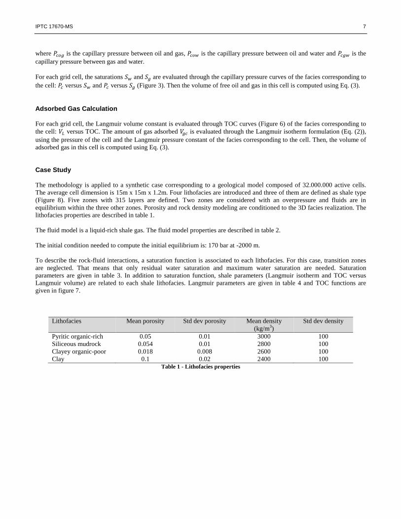
Case Study The methodology is applied to a synthetic case corresponding to a geological model composed of 32.000.000 active cells. The average cell dimension is 15m x 15m x 1.2m. Four lithofacies are introduced and three of them are defined as shale type (Figure 8). Five zones with 315 layers are defined. Two zones are considered with an overpressure and fluids are in equilibrium within the three other zones. Porosity and rock density modeling are conditioned to the 3D facies realization. The lithofacies properties are described in table 1. The fluid model is a liquid-rich shale gas. The fluid model properties are described in table 2. The initial condition needed to compute the initial equilibrium is: 170 bar at -2000 m. To describe the rock-fluid interactions, a saturation function is associated to each lithofacies. For this case, transition zones are neglected. That means that only residual water saturation and maximum water saturation are needed. Saturation parameters are given in table 3. In addition to saturation function, shale parameters (Langmuir isotherm and TOC versus Langmuir volume) are related to each shale lithofacies. Langmuir parameters are given in table 4 and TOC functions are given in figure 7.

Lithofacies Mean porosity Std dev porosity Mean density (kg/m3)

Std dev density

Pyritic organic-rich 0.05 0.01 3000 100 Siliceous mudrock 0.054 0.01 2800 100 Clayey organic-poor 0.018 0.008 2600 100 Clay 0.1 0.02 2400 100

Table 1 - Lithofacies properties

8 IPTC 17670-MS

Fluid Properties Gas density 0.812 kg/m3 Oil density 800.9 kg/m3 Condensate gas ratio 0.0037

Table 2 - Fluid properties

푆 푆 Pyritic organic-rich 0.3 0.5 Siliceous mudrock 0.25 0.6 Clayey organic-poor 0.22 0.4 Clay 0.26 1

Table 3 - Saturation values

Langmuir pressure : 푃 Pyritic organic-rich 27 bar Siliceous mudrock 27.5 bar Clayey organic-poor 28 bar Clay -

Table 4 - Langmuir pressure

Figure 7 - Langmuir Volume Constante vs. TOC

IPTC 17670-MS 9

Figure 8 - 3D properties description

10 IPTC 17670-MS

Figure 9 – An example of a cross section to visualize adsorbed GIIP

Results obtains are the volumes of fluids in place given table 5: STOIIP, free GIIP, adsorbed GIIP and GIIP (free and adsorbed) and 3D saturation and pressure of the different phases. An example of a cross section of 3D volume of adsorbed GIIP is given in figure 9.

Fluids in place STOIIP 58.9 106 sm3 GIIP - Free - Adsorbed

54.6 109 sm3 15.9 109 sm3 38.7 109 sm3

Table 5 - Fluids initially in place

The execution time to compute the volumes of fluids in place is 17 minutes with an Intel Corei5 CPU 2.53GHz using a specific plug-in of an industrial geological package1. Similar calculation with a classical black-oil simulator (Eclipse like) would take several hours of CPU time. Here, this computational speed allows performing of uncertainty analysis on multiple scenarios with multiple parameters. The uncertainty analysis has been done considering eight parameters: the seeds to generate lithofacies, porosity, rock density and TOC in the reservoir; a shift for each Langmuir Volume Constant vs. TOC curve; and a shift on pressure gradient in over pressured zones. This uncertainty analysis has been done using Monte-Carlo method. 500 samplings were performed on the parameters to predict the probability density corresponding to the volumes in place. The results are the probability density functions and cumulative distribution functions of free GIIP, adsorbed GIIP, GIIP (free + adsorbed) and STOIIP. Results of adsorbed gas initially in place are given figure 10.

Figure 10 – Probability density function (Green), cumulative distribution function (Red) and base value (Blue) of adsorbed GIIP

1 http://www.Terra3E.com/Software/Volumetrics/Shale_Volumetrics.html

IPTC 17670-MS 11

Integrated Workflow The calculation of volumes of fluids in place requires a large number of parameters (Figure 11): geological parameters, fluid parameters and relations modeling interactions between rocks and fluids. This paper focused on the calculation of hydrocarbon volumes of shale gas reservoir including adsorbed gas. As main parameter in the reserves evaluation of shale gas reservoir is the adsorbed gas in the matrix, any uncertainties in fluids in place estimates may involve large uncertainties on the reservoir production capability.

Figure 11 - Fluids-In-Place Calculation Workflow

Conclusions A complete methodology was developed to address this challenging task: 1) the calculations of free oil and gas initially in place based on the equilibrium between gravity and capillary forces; 2) the calculation of adsorbed gas using TOC and Langmuir isotherm. The proposed methodology does not estimate the fluids in place using stochastic simulation methods to distribute the fluid saturations spatially, but the method calculates rigorously these saturations using the correct physics of the phenomena. A high-resolution geological model is used to maintain the best accuracy without losing resolution due to upscaling. For each cell of the geological model, an exact volume calculation is performed, i.e. respecting all physics phenomena involved. This computational speed allows performing uncertainty analysis on multiple scenarios (e.g. “Optimistic”, “Average” and “Pessimistic”) and multiple parameters. Uncertainty analysis, especially on shale’s parameters, gives to the deciders a better assessment for designing their development plans including fracturation plan.

12 IPTC 17670-MS

Nomenclature

STOIIP = Stock Tank Oil Initially In Place GIIP = Gas Initially In Place TOC = Total Organic Carbon 퐵 = Formation volume factor of phase 훼 in the cell 푖 푔 = Gravitational constant 푃 = Pressure of the phase 훼 푃 = Capillary pressure between gas and water 푃 = Capillary pressure between oil and gas 푃 = Capillary pressure between oil and water 푃 = Capillary pressure 푃 = Pressure in the non-wetting phase 푃 = Pressure in the wetting phase 푃 = Langmuir pressure constant 푅 = Solution gas ratio 푅 = Condensate gas ratio 푆 = Saturation of phase 훼 in the cell 푖 푉 = Volume of the cell 푖 푉 = Adsorbed gas volume of the cell 푖 푉 = Langmuir volume constant 휑 = Porosity of the cell 푖 휌 = Rock density of the cell 푖 휌 = Reservoir oil density 휌 = Stock tank oil density 휌 = Reservoir gas density 휌 = Surface gas density 휌 = Surface condensate density

References Donnez, P. (2007). Essentials of reservoir engineering. Technip Editions.

Guérillot, D. and Bruyelle, J. Accurate Calculations of Stock Tank Oil Initially In Place (STOIIP) and Associated Uncertainties on High Resolution Geological Model, GEO-2012, 10th Middle East Geosciences Conference and Exhibition, 4-7 March 2012, Manama, Bahrain. Langmuir, I. (1918). The adsorption of gases on plane surfaces of glass, mica and platinum. Journal of the American Chemical society, 40(9), 1361-1403. Leahy-Dios, A., Das, M., Agarwal, A. and Kaminsky, R.D. Modeling of Transport Phenomena and Multicomponent Sorption for Shale Gas and Coalbed Methane in an Unstructured Grid Simulator. SPE 147352. SPE Annual Technical Conference and Exhibition, 30 October-2 November 2011, Denver, Colorado, USA. Ross, D. J., and Bustin, M.R. (2009). The importance of shale composition and pore structure upon gas storage potential of shale gas reservoirs. Marine and Petroleum Geology, 26(6), 916-927.