IPA Derivatives for Make-to-Stock Production-Inventory

IPA Derivatives for Make-to-Stock Production-Inventory Systems

With Lost Sales

Yao ZhaoBenjamin Melamed

Rutgers UniversityRutgers Business School – Newark and New Brunswick

Department of MSIS94 Rockafeller Rd.

Piscataway, NJ [email protected], [email protected]

Abstract

A stochastic fluid model (SFM) is a queueing model in which workload flow is modeled as fluidflow. More specifically, the traditional discrete arrival, service and departure stochastic processesare replaced by corresponding stochastic fluid-flow rate processes in an SFM. This paper appliesthe SFM paradigm to a class of single-stage, single-product Make-to-Stock (MTS) production-inventory systems with stochastic demand and random production capacity, where the finished-goods inventory is controlled by a continuous-time base-stock policy and unsatisfied demand islost. The paper derives formulas for IPA (Infinitesimal Perturbation Analysis) derivatives of thesample-path time averages of the inventory level and lost sales with respect to the base-stock leveland a parameter of the production rate process. These formulas are comprehensive in that theyare exhibited for any initial inventory state, and include right and left derivatives (when theydiffer). The formulas are obtained via sample path analysis under very mild assumptions, andare inherently nonparametric in the sense that no specific probability law need be postulated.It is further shown that all IPA derivatives under study are unbiased and very fast to compute,thereby providing the theoretical basis for on-line adaptive control of MTS production-inventorysystems.

Keywords and Phrases: Infinitesimal Perturbation Analysis, IPA, IPA derivatives, IPAgradients, Lost Sales, Make-to-Stock, production-inventory systems, stochastic fluid models,SFM.

1 Introduction

Production-inventory systems consist of production facilities that feed replenishment product toinventory facilities, driven by random demand and possibly random production processes, as well asfeedback information from inventory to production facilities. An important instance of production-inventory systems is the Make-to-Stock (MTS) class, where the inventory facility sends its stateinformation to the production facility as a control signal, which modulates production with the aimof maintaining the inventory level at a prescribed level, called base-stock level. Such systems canadmit backorders when stock is depleted, or suffer lost sales. This paper treats MTS systems withlost sales (see Section 2), and is a sequel to Zhao and Melamed (2005), which treats MTS systemswith backorders.

Economic considerations in supply chains call for effective control of inventory levels and pro-duction rates, in order to optimize some prescribed performance metrics. In many real worldapplications, the underlying demand and production processes may be subject to time varyingprobability laws. This motivates on-line algorithms that can adaptively control such systems overtime with the objective of minimizing inventory on-hand without compromising customer servicemetrics. To this end, we propose to use IPA (Infinitesimal Perturbation Analysis) derivatives ofselected random variables [for comprehensive discussions of IPA derivatives and their applications,refer to Glasserman (1991), Ho and Cao (1991) and Fu (1994a, 1994b)]. IPA derivatives providesensitivity information on system metrics with respect to control parameters of interest, and assuch can serve as the theoretical underpinnings for on-line control algorithms. Specifically, let L(θ)be a random variable, parameterized by a generic real-valued parameter θ chosen from a closedand bounded set Θ. The IPA derivative (gradient) of L(θ) with respect to θ is the random variable

L′(θ) =

d

dθL(θ), provided that it exists almost surely. Furthermore, L

′(θ) is said to be unbiased,

if the expectation and differentiation operators commute, namely, E[d

dθL(θ)] =

d

dθE[L(θ)]; other-

wise, it is said to be biased. Sufficient conditions for unbiased IPA derivatives are given in thefollowing lemma

Fact 1 (see Rubinstein and Shapiro (1993), Lemma A2, p. 70)

An IPA derivative L′(θ) is unbiased, if

(a) For each θ ∈ Θ, the IPA derivatives L′(θ) exist w.p.1 (with probability 1).

(b) W.p.1, L(θ) is Lipschitz continuous in Θ, and the (random) Lipschitz constants have finitefirst moments. �

Comprehensive discussions of IPA derivatives and their applications can be found in Glasserman(1991), Ho and Cao (1991) and Fu (1994).

Most papers on production-inventory systems (and MTS systems in particular) postulate spe-cific probability laws that govern the underlying stochastic processes (e.g., Poisson demand arrivalsand exponential service times). For simple systems, such as the one-stage MTS variety, closed-formformulas of key performance metrics (e.g., statistics of inventory levels and lost sales or backorders)have been derived as functions of control parameters. For example, Zipkin (1986) and Karmarkar(1987) obtain the optimal control of these systems with respect to batch sizes and re-order points bystandard optimization techniques. For more complex MTS systems, such as the multi-stage serialvariety, closed-form formulas are not available. A sample path analysis is carried out by Buza-cott, Price and Shanthikumar (1991) for a 2-stage production system which is governed by the

1

continuous-time base-stock policy. Diffusion models and deterministic fluid models have been pro-posed in order to mitigate the analytical and computational complexity of performance evaluationand optimal control. For example, Wein (1992) used a diffusion process to model a multi-product,single-server MTS system, while Veatch (2002) discussed diffusion and fluid-flow models of serialMTS systems. Note, however, that diffusion models require a heavy traffic condition in order to bevalid approximations (Wein 1992). In a similar vein, while deterministic fluid-flow models providevaluable insights into the control rules of such systems, deterministic modeling may well result insubstantial numerical errors (Veatch 2002).

Simulation has been widely used to study the performances of complex production-inventorysystems under uncertainty. Glasserman and Tayur (1995) considered a class of production-inventorysystems under the so-called periodic-review, modified base-stock policy, and estimated its perfor-mance metrics and IPA derivatives using simulation. While periodic-review policies evaluate systemperformance at discrete review times, discrete-event simulation, in contrast, can track system per-formance continuously, but this can be overly time consuming for large-scale systems, due to thelarge number of events that need to be processed (e.g., arrivals and service completions). All in all,most papers on stochastic production-inventory systems postulate a specific underlying probabilitylaw, and focus on off-line control and optimization algorithms.

Recent work has sought to address these shortcomings in the context of fluid-flow queueingsystems, and especially, the stochastic fluid model (SFM) setting, where transactions carry fluidworkload, random discrete arrivals become random arrival rates and random discrete services be-come random service rates. SFM-like settings represent an alternative (continuous or fluid-flow)queueing paradigm, which differs from the traditional (discrete) queueing paradigm in the wayworkload is transported in the system1. Both paradigms are set in a network of nodes, each ofwhich houses a server and a buffer, where network sources and sinks are viewed as exogenous nodes,and all others as endogenous nodes. Transactions representing parcels of workload arrive at thenetwork from some source, traverse the network according to some itinerary, and then depart thenetwork at some sink. The two queueing paradigms differ, however, in the way workload movesin the system. In the discrete queueing paradigm, transaction workload moves “abruptly” amongnodes following a service time, while in the continuous queueing paradigm, transaction workloadmoves “gradually” (i.e., flows like fluid) for the duration of its service time.

A heuristic modeling rationale underlying SFM systems is the assumption that individual trans-actions carry miniscule workload as compared to the entire transaction flow, so the effect of indi-vidual transactions is infinitesimal and akin to “molecules” in a fluid flow. Furthermore, in manycases, a transaction workload does move gradually from one node to another, rather than abruptly(e.g., a conveyor belt carrying bulk material, loading and unloading a truck, train, etc.) In fact,discrete queueing systems can be abstracted as “limiting cases” of continuous queueing systems,where the flow rate is zero when a transaction is still, but at the moment of motion the flow ratebecomes momentarily infinite; in other words, the flow rate is akin to a Dirac function. Pursu-ing this line of reasoning, the “Dirac pulses” of flow rates in a discrete queueing system can beapproximated by high flow rates of short duration in a continuous queueing system. Whicheverreasoning is used, the modeler can often choose to model a queueing system using either paradigmon equal footing. Finally, we point out that ceteris paribus, SFM systems enjoy an importantadvantage over their discrete counterparts: IPA derivatives in SFM setting are unbiased, whiletheir counterparts in discrete queueing systems are by and large biased (Heidelberger et al. 1988).Thus, the local shape of sample paths in the fluid-flow paradigm confers technical advantages on

1For simplicity we address only open networks in this discussion.

2

them. IPA derivatives, derived in SFM setting, can provide important information and insights fortheir discrete counterparts, by applying derivative formulas obtained in SFM setting to queueingsystems that have been traditionally viewed as belonging to the discrete queueing paradigm. Whilepreliminary unpublished work by one of the authors suggests that this approach is viable, morework is needed to establish its broad applicability.

Motivated by the considerations above, Wardi et al. (2002) derived IPA derivatives in SFMsetting; we henceforth refer to this approach as IPA-over-SFM. Wardi et al. (2002) consideredtwo performance metrics: loss volume and buffer-workload time average; each of these metrics wasdifferentiated with respect to buffer size, a parameter of the arrival rate process and a parameter ofthe service rate process. The paper showed the IPA derivatives to be unbiased, easily computableand nonparametric. Consequently, these derivatives can be computed in simulations, or in thefield, and the values can have potential applications to on-line control and stochastic optimization.Paschalidis et al. (2004) treated multi-stage MTS production-inventory systems with backordersin SFM setting. Assuming that inventory at each stage is controlled by a continuous-time base-stock policy, the paper computed the right IPA derivatives of the time averaged inventory level andservice level with respect to base-stock levels, and used them to determine the optimal base-stocklevels at each stage. Zhao and Melamed (2004) applied the IPA-over-SFM approach to a classof single-product, single-stage MTS systems with backorders, and derived IPA formulas for thetime averages of inventory level and backorder level with respect to the base-stock level, as wellas a parameter of the production rate process. It should be pointed out that Wardi et al. (2002),Paschalidis et al. (2004) and Zhao and Melamed (2004) assume that systems start with certaininitial inventory states, and only consider cases where the left and right IPA derivatives coincide.In contrast, Zhao and Melamed (2005) considered any initial inventory state and derived sided IPAderivative formulas where needed, thereby providing the theoretical basis for IPA-based on-linecontrol of MTS systems with backorders.

The goal of this paper is to derive IPA derivatives for MTS systems with lost-sales, and toshow them to be unbiased. The paper makes the following contributions. First, we derive IPAderivative formulas for two metrics, the inventory-level time average and lost-sales time average,with respect to the base-stock level for all initial inventory states, including sided derivatives whenthey differ. We are only aware of one paper [Wardi et al. (2002)] addressing IPA-over-SFM queueswith finite buffers, which can be used to model MTS systems with lost sales. But unlike the currentpaper, Wardi et al. (2002) limits the initial condition to an empty buffer. Second, we derive IPAderivative formulas for the aforementioned metrics with respect to a production rate parameter,including sided derivatives when they differ. In contrast, Wardi et al. (2002) only considers caseswhere the left and right IPA derivatives coincide (in fact, the left and right IPA derivatives maydiffer). The computation of the general IPA derivatives for any initial inventory state and forcases where the left and right IPA derivatives may differ requires major extensions of the currentresults in the literature. As will become evident in the sequel, MTS systems with lost-sales arealso analytically more challenging than MTS systems with backorders, a fact that results in moreelaborate formulas.

The merit of our contribution stems from potential applications of IPA derivatives to on-linecontrol of MTS systems. Clearly, IPA-based on-line control applications mandate the computationof IPA derivatives for all initial inventory states, as well as all sided derivatives when they differ,since a control action can change system parameters at a variety of system states (which are thenconsidered as new initial states). Moreover, it obviously makes little or no sense to wait for thesystem to return to selected inventory states for which IPA derivatives are known, as this couldsuspend control actions over extended periods of time. To summarize, for IPA-based applications

3

to be general and efficacious, it is necessary that the requisite IPA derivative formulas satisfy thefollowing requirements:

1. For usability, they should be comprehensive in the sense that they are valid for any initialcondition of the system. In addition, if a left-derivative does not coincide with its right-derivative counterpart, then both should be exhibited.

2. For statistical accuracy, they should be unbiased.

3. For generality, they should be nonparametric in the sense that they are solely computable fromthe sample path observed without making any distributional assumptions on the underlyingprobability law.

4. To enable on-line applications, they should be fast to compute.

To this end, this paper derives all sided IPA derivatives for MTS systems with lost-sales for anyinitial inventory state. It further shows these IPA derivatives to be unbiased, nonparametric, andeasy to compute, which facilitates on-line control applications.

Throughout the paper, we use the following notational conventions and terminology. Theindicator function of set A is denoted by 1A, and x+ = max{x, 0}. A function f(x) is said tobe locally differentiable at x if it is differentiable in a neighborhood of x; it is said to be locallyindependent of x if is constant in a neighborhood of x.

The rest of the paper is organized as follows. Section 2 presents the production-inventorymodels under study. Section 3 provides variational bounds for system metrics. Section 4 derivesIPA derivative formulas and shows them to be unbiased. Finally, Section 5 concludes the paper.

2 The Make-to-Stock Model With Lost Sales

Consider the traditional single-stage, single-product MTS system, consisting of a production facilityand an inventory facility. The two facilities interact: the latter sends back orders to the former,while the former produces stock to replenish the latter. The production facility is comprised ofa queue that houses a production server (a single machine, a group of machines or a productionline), preceded by an infinite buffer that holds incoming production orders. We assume that theproduction facility has an unlimited supply of raw material, so it never starves. The inventoryfacility satisfies incoming demands on a first come first serve (FCFS) basis, and is controlled by acontinuous-time base-stock policy with some base-stock level S > 0 (the case S = 0 corresponds toa just-in-time system and its treatment is a simple special case.) More specifically, the inventoryand production facilities are coupled, and operate in two modes as follows:

Normal operational mode. While the inventory level does not exceed S, the inventory facilityplaces the orders of incoming demands as discrete production jobs in the production facility’sbuffer according to some operational rule (to be detailed below). The production facility fillsthese outstanding orders and replenishes the inventory facility back to its base-stock level,but no higher. We refer to this operational mode as normal operation, because the systemstrives to reach an inventory level S, and in so doing, it maintains an inventory level notexceeding S.

Overage operational mode. While the inventory level exceeds S (this could happen, for exam-ple, as a result of a control action that lowered S), the production facility buffer is empty,

4

Figure 1: The Make-to-Stock production-inventory system with lost sales

so production is temporarily suspended until the inventory level reaches or crosses S fromabove, at which point normal operation is resumed. We refer to this operational mode asoverage operation, because it allows the system to adapt to a lower base-stock level, S, aimingto enter normal operation.

The demand process consists of an interarrival-time process of demands and their randommagnitude. Demands arrive at the inventory facility and are satisfied from inventory on hand (ifavailable). Otherwise, when an inventory shortage is encountered, the behavior of the MTS queueis governed by the lost-sales rule as follows: The incoming demand is satisfied by the amount ofinventory on hand, and any shortage of inventory becomes a lost sale. Thus, the system’s overallactions aim to move the inventory level to the base-stock level, S.

2.1 Mapping MTS Systems to SFM Versions

We next proceed to map the traditional discrete MTS system with lost sales into an SFM version,as depicted in Figure 1. Level-related stochastic processes are mapped into fluid versions of theirtraditional counterparts in a natural way, as follows:

Inventory level. The traditional jump process of the level of inventory on hand at the inventoryfacility is mapped to a fluid-level counterpart, {I(t)}, where I(t) is the (fluid) volume ofinventory on-hand at time t.

Outstanding orders. The traditional jump process of the level of outstanding orders in the bufferof the production facility is mapped to a fluid-level counterpart, {X(t)}, where X(t) is the(fluid) volume of outstanding orders at time t.

Traffic-related stochastic processes in Figure 1 are mapped into fluid versions of their traditionalcounterparts, as follows:

Arrival rate. The traditional arrival process of discrete demands at the inventory facility ismapped to a fluid-flow stochastic process, {α(t)}, where α(t) is the rate of incoming demandsat time t.

5

Production rate. The traditional service (production) process of discrete product at the produc-tion facility is mapped to a fluid-flow stochastic process, {µ(t)}, where µ(t) is the productionrate at time t.

Loss rate. The traditional loss process of discrete sales at the inventory facility is mapped to afluid-flow stochastic process, {ζ(t)}, where ζ(t) is the (fluid) loss rate of sales at time t.

Outstanding order rate. The traditional arrival process of signals for placing discrete outstand-ing orders at the production facility is mapped to a fluid-flow stochastic process, {λ(t)}, whereλ(t) is the rate of incoming outstanding orders at time t.

Replenishment rate. The traditional traffic process of discrete replenished product from theproduction facility to the inventory facility is mapped to a fluid-flow stochastic process, {ρ(t)},where ρ(t) is the traffic rate of product at time t.

We now proceed to exhibit the formal definitions of all fluid-model components of the MTSsystem with lost sales.

During overage operation, the inventory process is governed by the one-side stochastic differen-tial equation

d

dt+I(t) = −α(t), (2.1)

and

ζ(t) = 0, (2.2)

X(t) = 0. (2.3)

During normal operation, the model satisfies the conservation relation,

X(t) + I(t) = S. (2.4)

The outstanding orders process is governed by the sided stochastic differential equation,

dX(t)dt+

=

⎧⎪⎨⎪⎩

0, X(t) = 0 and α(t) ≤ µ(t)0, X(t) = S and α(t) ≥ µ(t)α(t) − µ(t), otherwise

(2.5)

The lost-sales rate process is given by

ζ(t) = [α(t) − µ(t)] 1{I(t)=0,α(t)>µ(t)}, t ≥ 0. (2.6)

The arrival-rate process of outstanding orders is given by

λ(t) =

⎧⎪⎨⎪⎩

0, if I(t) > Sµ(t), if I(t) = 0 and α(t) > µ(t)α(t), otherwise

(2.7)

and the replenishment-rate process is given by

ρ(t) =

{µ(t), if X(t) > 0min{µ(t), λ(t)}, if X(t) = 0.

(2.8)

6

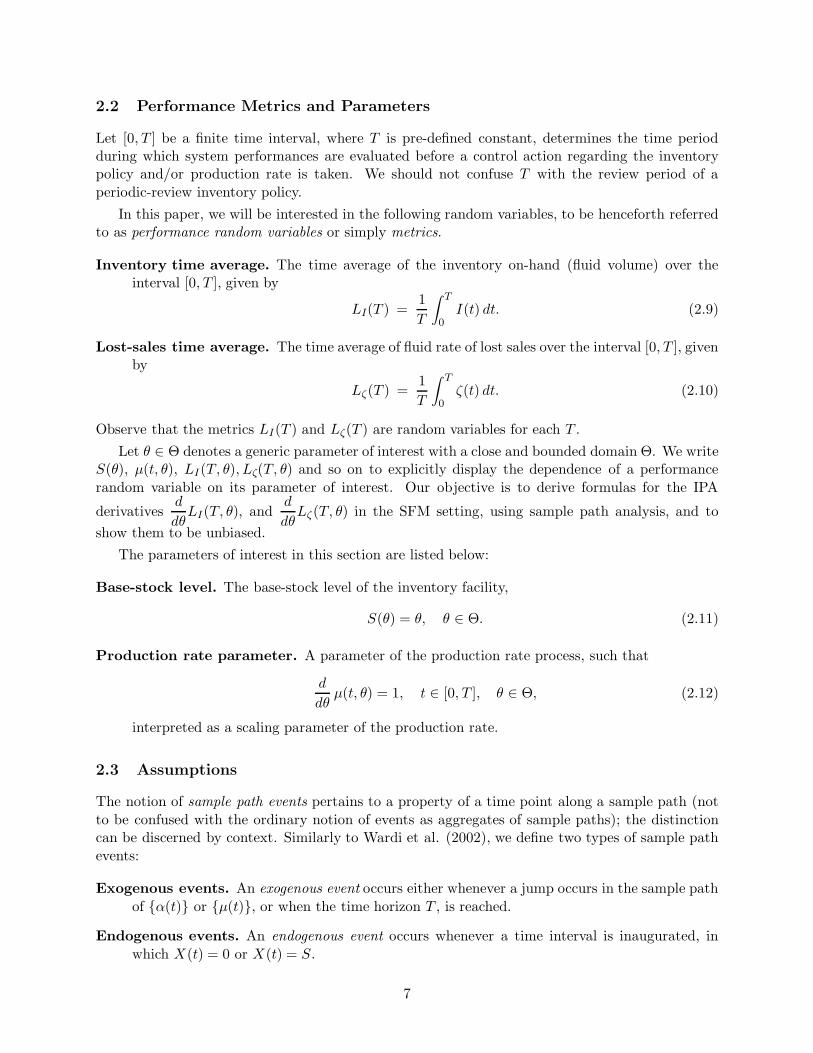
2.2 Performance Metrics and Parameters

Let [0, T ] be a finite time interval, where T is pre-defined constant, determines the time periodduring which system performances are evaluated before a control action regarding the inventorypolicy and/or production rate is taken. We should not confuse T with the review period of aperiodic-review inventory policy.

In this paper, we will be interested in the following random variables, to be henceforth referredto as performance random variables or simply metrics.

Inventory time average. The time average of the inventory on-hand (fluid volume) over theinterval [0, T ], given by

LI(T ) =1T

∫ T

0I(t) dt. (2.9)

Lost-sales time average. The time average of fluid rate of lost sales over the interval [0, T ], givenby

Lζ(T ) =1T

∫ T

0ζ(t) dt. (2.10)

Observe that the metrics LI(T ) and Lζ(T ) are random variables for each T .Let θ ∈ Θ denotes a generic parameter of interest with a close and bounded domain Θ. We write

S(θ), µ(t, θ), LI(T, θ), Lζ(T, θ) and so on to explicitly display the dependence of a performancerandom variable on its parameter of interest. Our objective is to derive formulas for the IPA

derivativesd

dθLI(T, θ), and

d

dθLζ(T, θ) in the SFM setting, using sample path analysis, and to

show them to be unbiased.The parameters of interest in this section are listed below:

Base-stock level. The base-stock level of the inventory facility,

S(θ) = θ, θ ∈ Θ. (2.11)

Production rate parameter. A parameter of the production rate process, such that

d

dθµ(t, θ) = 1, t ∈ [0, T ], θ ∈ Θ, (2.12)

interpreted as a scaling parameter of the production rate.

2.3 Assumptions

The notion of sample path events pertains to a property of a time point along a sample path (notto be confused with the ordinary notion of events as aggregates of sample paths); the distinctioncan be discerned by context. Similarly to Wardi et al. (2002), we define two types of sample pathevents:

Exogenous events. An exogenous event occurs either whenever a jump occurs in the sample pathof {α(t)} or {µ(t)}, or when the time horizon T , is reached.

Endogenous events. An endogenous event occurs whenever a time interval is inaugurated, inwhich X(t) = 0 or X(t) = S.

7

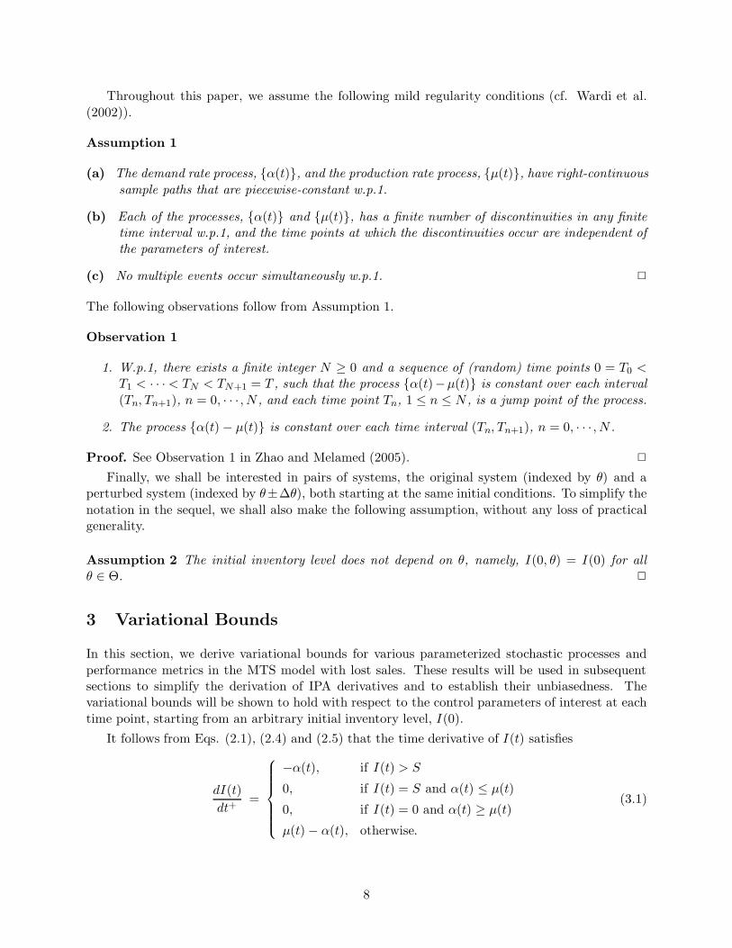
Throughout this paper, we assume the following mild regularity conditions (cf. Wardi et al.(2002)).

Assumption 1

(a) The demand rate process, {α(t)}, and the production rate process, {µ(t)}, have right-continuoussample paths that are piecewise-constant w.p.1.

(b) Each of the processes, {α(t)} and {µ(t)}, has a finite number of discontinuities in any finitetime interval w.p.1, and the time points at which the discontinuities occur are independent ofthe parameters of interest.

(c) No multiple events occur simultaneously w.p.1. �

The following observations follow from Assumption 1.

Observation 1

1. W.p.1, there exists a finite integer N ≥ 0 and a sequence of (random) time points 0 = T0 <T1 < · · · < TN < TN+1 = T , such that the process {α(t)−µ(t)} is constant over each interval(Tn, Tn+1), n = 0, · · · , N , and each time point Tn, 1 ≤ n ≤ N , is a jump point of the process.

2. The process {α(t) − µ(t)} is constant over each time interval (Tn, Tn+1), n = 0, · · · , N .

Proof. See Observation 1 in Zhao and Melamed (2005). �

Finally, we shall be interested in pairs of systems, the original system (indexed by θ) and aperturbed system (indexed by θ±∆θ), both starting at the same initial conditions. To simplify thenotation in the sequel, we shall also make the following assumption, without any loss of practicalgenerality.

Assumption 2 The initial inventory level does not depend on θ, namely, I(0, θ) = I(0) for allθ ∈ Θ. �

3 Variational Bounds

In this section, we derive variational bounds for various parameterized stochastic processes andperformance metrics in the MTS model with lost sales. These results will be used in subsequentsections to simplify the derivation of IPA derivatives and to establish their unbiasedness. Thevariational bounds will be shown to hold with respect to the control parameters of interest at eachtime point, starting from an arbitrary initial inventory level, I(0).

It follows from Eqs. (2.1), (2.4) and (2.5) that the time derivative of I(t) satisfies

dI(t)dt+

=

⎧⎪⎪⎪⎪⎪⎨⎪⎪⎪⎪⎪⎩

−α(t), if I(t) > S

0, if I(t) = S and α(t) ≤ µ(t)

0, if I(t) = 0 and α(t) ≥ µ(t)

µ(t) − α(t), otherwise.

(3.1)

8

3.1 Variational Bounds With Respect to the Base-Stock Parameter

In this section, the IPA parameter of interest is S(θ) = θ for θ ∈ Θ. Let {I(t, θ)} be the inventorylevel process in an MTS system with lost-sales, where θ ∈ Θ and I(0, θ) = I(0). Then, Eq. (3.1)induces a (random) partition of the interval [0, T ], given by

R(θ) = {R1(θ),R2(θ),R3(θ),R4(θ)}, (3.2)

where each region, Rk(θ), 1 ≤ k ≤ 4, is defined as follows,

R1(θ) = {t ∈ [0, T ] : I(t, θ) = 0 and α(t) ≥ µ(t)},R2(θ) = {t ∈ [0, T ] : [I(t, θ) = 0 and α(t) < µ(t)]

or [I(t, θ) = S(θ) and α(t) > µ(t)] or 0 < I(t, θ) < S(θ)},R3(θ) = {t ∈ [0, T ] : I(t, θ) = S(θ) and α(t) ≤ µ(t)},R4(θ) = {t ∈ [0, T ] : I(t, θ) > S(θ)}.

We first prove the variational bounds for the inventory level process, {I(t, θ)}.

Proposition 1 For an MTS system with the lost-sales rule, let θ1, θ2 ∈ Θ. Then,

0 ≤ |I(t, θ1) − I(t, θ2)| ≤ |θ1 − θ2|, t ∈ [0, T ]. (3.3)

Proof. Recall that by Assumption 2,

I(0, θ1) = I(0, θ2) = I(0). (3.4)

Clearly, Eqs. (3.4) and (3.1) imply the result trivially for θ1 = θ2. It remains to show the resultfor the case θ1 �= θ2. Without loss of generality, we assume that θ1 < θ2, and show that

0 ≤ I(t, θ2) − I(t, θ1) ≤ θ2 − θ1, t ∈ [0, T ]. (3.5)

To this end, we first prove the lefthand side of inequality (3.5) by showing that whenever I(t, θ1) =

I(t, θ2) for any t ∈ [0, T ], one hasd

dt+[I(t, θ2) − I(t, θ1)] ≥ 0.

An examination of Eq. (3.1) reveals that the equality I(t, θ1) = I(t, θ2) can take place only inthe following cases.

Case 1: t ∈ Rk(θ1)⋂Rk(θ2) for some 1 ≤ k ≤ 4. In this case, we immediately have

d

dt+[I(t, θ2)−

I(t, θ1)] = 0.

Case 2: t ∈ R3(θ1)⋂R2(θ2). In this case, I(t, θ1) = I(t, θ2) = S(θ1) = θ1 and

d

dt+[I(t, θ2) −

I(t, θ1)] = µ(t) − α(t) ≥ 0, where the inequality follows from the definition of R3(θ1).

Case 3: t ∈ R4(θ1)⋂R2(θ2). In this case,

d

dt+[I(t, θ2) − I(t, θ1)] = µ(t) ≥ 0 by the definition of

R2(θ2) and R4(θ1).


d

dt+[I(t, θ2) − I(t, θ1)] = α(t) ≥ 0 by the definition of

R3(θ2) and R4(θ1).

9

The lefthand side of inequality (3.5) follows from Eq. (3.4) and by the continuity of the realizationsof the inventory level process.

To prove the righthand side of inequality (3.5), we examine the behavior of {I(t, θ2)− I(t, θ1)}in the four regions of the partition (3.2). Informally, the proof characterizes {I(t, θ2)− I(t, θ1)} forall pairs of regions in the partitions associated with each θ, such that I(t, θ1) is in one region andI(t, θ2) is in the other. More formally, the characterization covers t in all intersections of the formRi(θ1)

⋂Rj(θ2), 1 ≤ i, j ≤ 4. Note that the intersections partition the interval [0, T ] and theirnumber is finite w.p.1 by Part (b) of Assumption 1. The proof proceeds in two steps. In the firststep, we consider the extremal open set (a, b) of any such intersection. We then show that if

I(a, θ2) − I(a, θ1) ≤ θ2 − θ1, (3.6)

thenI(t, θ2)− I(t, θ1) ≤ θ2 − θ1, a < t < b. (3.7)

By continuity of the inventory level process, the inequality (3.7) will then extend to the interval[a, b]. In the second step, we order the intervals (ak, bk) contiguously, and prove the inequality (3.5)throughout [0, T ], by a straightforward induction on k, where the induction basis holds by Eq.(3.4),and the induction step is immediate from the contiguity of the ordered intersections.

The following observation reduces substantially the number of region-pair cases (intersections)to be checked. There is no need to check for pairs of regions with the same subscript, i = j, since

in their intersectiond

dt+[I(t, θ2) − I(t, θ1)] = 0 trivially, which implies that I(t, θ2) − I(t, θ1) is

constant in the intersection. It remains to check the following list of cases.


d

dt+[I(t, θ2) − I(t, θ1)] = µ(t) − α(t) ≤ 0, where the

inequality follows from the definition of R1(θ1). In view of (3.6), inequality (3.7) immediatelyfollows.


d

dt+[I(t, θ2) − I(t, θ1)] = 0.

Case 3: t ∈ R3(θ1)⋂R2(θ2). In this case, I(t, θ2) ≤ θ2 and I(t, θ1) = θ1, which implies that

I(t, θ2)− I(t, θ1) ≤ θ2 − θ1.

Case 4: t ∈ R4(θ1)⋂R2(θ2). In this case, I(t, θ2) ≤ θ2 and θ1 < I(t, θ1), which implies that

I(t, θ2)− I(t, θ1) ≤ θ2 − θ1.

Case 5: t ∈ R4(θ1)⋂R3(θ2). In this case, I(t, θ2) = θ2 and θ1 < I(t, θ1), which implies that

I(t, θ2)− I(t, θ1) ≤ θ2 − θ1.

The proof is complete. �

We next derive variational bounds for the time average of lost sales. To this end, we defineK(T, θ) to be the number of extremal subintervals of [0, T ] in which I(t, θ) = 0.

Proposition 2 For an MTS system with the lost-sales rule, let θ1, θ2 ∈ Θ. Then,∫ T

0|ζ(t, θ1) − ζ(t, θ2)| dt ≤ max{K(T, θ1), K(T, θ2)}|θ1 − θ2|. (3.8)

10

Proof. The case of θ1 = θ2 is trivial, so it remains to prove the case θ1 �= θ2, and assume θ1 < θ2

without loss of generality. We prove the following inequality,

0 ≤∫ T

0[ζ(t, θ1) − ζ(t, θ2)] dt ≤ K(T, θ1)[θ2 − θ1], (3.9)

which is stronger than the requisite result.Since θ1 < θ2, the proof of Proposition 1 implies that I(t, θ1) ≤ I(t, θ2) for all t ∈ [0, T ].

Consequently, ζ(t, θ2) ≤ ζ(t, θ1) for all t ∈ [0, T ], which establishes the lefthand side of (3.9).We next prove the righthand side of inequality (3.9). In view of the inequality I(t, θ1) ≤ I(t, θ2)

for all t ∈ [0, T ], it suffices to show that for any extremal subinterval [U, V ] of [0, T ] in whichI(t, θ1) = 0, one has

∫ t

U[ζ(τ, θ1)− ζ(τ, θ2)] dτ ≤ I(U, θ2) − I(U, θ1), t ∈ [U, V ]. (3.10)

Define W ∈ [U, V ] to be the first time point at which I(t, θ2) = 0, if it exists; otherwise, de-fine W = V . Since I(t, θ1) = I(t, θ2) = 0 for t ∈ [W, V ), it follows from Eq. (2.6) that∫ V

W[ζ(τ, θ1) − ζ(τ, θ2)] dτ = 0, so it remains to consider the interval [U, W ). But for any t ∈ [U, W ),

ζ(t, θ2) = 0 and ζ(t, θ1) = α(t) − µ(t). Hence, for every t ∈ [U, W ),∫ t

U[ζ(τ, θ1) − ζ(τ, θ2)] dτ =

∫ t

U[α(τ) − µ(τ)] dτ.

We conclude that for every t ∈ [U, W ),∫ t

U[α(τ)− µ(τ)] dτ = I(U, θ2) − I(t, θ2) ≤ I(U, θ2) − I(U, θ1) ≤ θ2 − θ1,

where the equality is due to the dynamics of Eq. (3.1), the first inequality follows from the relationI(t, θ2) ≥ I(U, θ1) = 0, and the second inequality follows from (3.5). The result now followsby applying inequality (3.10) to all extremal subintervals of the form [U, V ] and summing thecorresponding inequalities. �

3.2 Variational Bounds With Respect to a Production Rate Parameter

In this section, the IPA parameter of interest is a parameter, θ, of the production rate process,{µ(t, θ)}, satisfying Eq. (2.12). Our results build upon prior results in Wardi and Melamed (2001),which assume a special initial condition for the workload.

Observation 2 For an MTS system with the lost-sales rule, the stochastic differential equationsgoverning the outstanding orders process {X(t)} in normal operation, the loss-rate process, {ζ(t)},and the replenishment rate process, {ρ(t)}, are identical to those governing the buffer workload,overflow and outflow processes, respectively, in the SFM queuing system studied in Wardi et al.(2001).

Proof. Follows from the fact that we can identify the demand arrival rate process, productionrate process, and base-stock level parameter, respectively, with the inflow rate process, service rateprocess and buffer capacity parameter in Wardi and Melamed (2001). �

11

For notational convenience, we define an auxiliary process, called the extended outstandingorders process, {Y (t, θ)}, by

Y (t, θ) =

{S − I(t, θ), if I(t, θ) > S (overage operation)

X(t, θ), if I(t, θ) ≤ S (normal operation)(3.11)

Observe that Y (t) is negative during overage operation and non-negative during normal operation.Furthermore, Eq. (2.4) implies the conservation relation,

I(t, θ) + Y (t, θ) = S, t ≥ 0, (3.12)

valid for each operational mode (overage and normal).

Proposition 3 For an MTS system with the lost-sales rule, let θ1, θ2 ∈ Θ. Then,

max{|Y (t, θ1) − Y (t, θ2)| : t ∈ [0, T ]} ≤ T |θ1 − θ2|and ∫ T

0|ζ(t, θ1) − ζ(t, θ2)| dt ≤ 2 T |θ1 − θ2|.

Proof. By Assumption 2 and Eq. (3.12), Y (0, θ1) = Y (0, θ2). In view of the fact that {Y (t, θ1)} and{Y (t, θ2)} coincide during overage operation, it suffices to assume that the system starts in normaloperation, namely, Y (0, θ1) = Y (0, θ2) ≥ 0. The results follow immediately from Proposition 3.2of Wardi and Melamed (2001), since the proof there is readily seen to hold for any initial state innormal operation. �

Corollary 1 For an MTS system with the lost-sales rule, let θ1, θ2 ∈ Θ. Then,

|I(t, θ1) − I(t, θ2)| ≤ T |θ1 − θ2|, t ∈ [0, T ].

Proof. Eq. (3.12) and Proposition 3 imply that

|I(t, θ1)− I(t, θ2)| = |[S − Y (t, θ1)]− [S − Y (t, θ2)]| ≤ T |θ1 − θ2|.�

4 IPA Derivatives

We are now in a position to derive IPA derivatives for various parameterized stochastic processesand performance metrics in the MTS model subject to lost sales rule. We mention in passing thatsuch systems are analytically more challenging than MTS systems with backorders, because theinventory state of the former has an extra boundary. More specifically, while the inventory stateof both systems is bounded from above by S, that of MTS systems with lost sales is also boundedfrom below by 0.

Let (Qj(θ), Rj(θ)), j = 1, . . . , J(θ) be the ordered extremal subintervals of [0,∞), such thatI(t, θ) < S for all t ∈ (Qj, Rj), that is,the endpoints, Qj(θ) and Rj(θ), are obtained via inf andsup functions, respectively. By convention, if any of these endpoints does not exist, then it is setto ∞. Furthermore, we let Zj(θ) ∈ (Qj(θ), Rj(θ)) be the first time point in this interval at whichI(t, θ) = 0 if such a point exists; otherwise, let Zj(θ) = Rj(θ).

12

Observation 3

Q1(θ) < R1(θ) < Q2(θ) < R2(θ) < . . . < QJ(θ)(θ) < RJ(θ)(θ). (4.1)

Proof. See Observation 3 in [19]. �

4.1 IPA Derivatives with Respect to the Base-Stock Level

This section treats IPA derivatives (including sided ones) for the inventory time average, LI(T, θ),and the lost-sales time average, Lζ(T, θ), both with respect to the base-stock level, S, and exhibitstheir formulas for any initial inventory state. We first prove a number of useful lemmas that simplifythe proofs of the main results later in this section. We then proceed to obtain the IPA derivativesfor LI(T, θ) by first obtaining those for the inventory process, {I(t, θ)}, following which we obtainthe IPA derivatives for Lζ(T, θ). Finally, we establish the unbiasedness of all the IPA derivativesabove.

Assumption 3

(a) S(θ) = θ, where θ ∈ Θ.

(b) The processes {α(t)} and {µ(t)} are independent of the parameter θ. �

The following lemma provides basic properties for the inventory level process.

Lemma 1

(a) For every j ≥ 1,d

dθI(t, θ) = 1, t ∈ [Rj(θ), Zj+1(θ)).

(b) For every j ≥ 1,d

dθI(t, θ) = 0, t ∈ (Zj(θ), Rj(θ)).

Proof. To prove part (a), note that each Rj(θ), j ≥ 1 is locally differentiable with respect to θ bypart (c) of Assumption 1. By Observation 3, Rj(θ) < Qj+1(θ), where Qj+1(θ) is a jump point of{α(t) − µ(t)}, and therefore Qj+1(θ) is locally independent of θ. Consequently, I(t, θ) = S(θ) fort ∈ (Rj(θ), Qj+1(θ)] and

I(t, θ) = S(θ) +∫ t

Qj+1(θ)[µ(t) − α(t)] dt, t ∈ (Qj+1(θ), Zj+1(θ)).

Part (a) now follows by differentiating I(t, θ) with respect to θ for t ∈ (Rj(θ), Zj+1(θ)].To prove part (b), consider first the extremal time interval [Zj(θ), Z̃j(θ)] in which I(t, θ) = 0.

By part (c) of Assumption 1, Zj(θ) is locally differentiable with respect to θ, Z̃j(θ) is a jump pointof {α(t) − µ(t)} and Zj(θ) < Z̃j(θ). Therefore, Z̃j(θ) is locally independent of θ and I(t, θ) = 0

is locally independent of θ for t ∈ (Zj(θ), Z̃j(θ)]. Finally, note that by Eq. (3.1),d

dt+I(t, θ) is

independent of θ for t ∈ (Z̃j(θ), Rj(θ)). The proof is now complete. �

The following lemma provides basic properties for the time average of lost sales.

13

Lemma 2 Let 0 ≤ u ≤ T be a time point, independent of θ.

(a) For every j = 1, . . . , J(θ), on the event {Zj(θ) = Rj(θ)},d

dθ

∫ u

Qj(θ)ζ(t, θ) dt = 0, for Qj(θ) < u ≤ Rj(θ) (4.2)

(b) For every j = 2, . . . , J(θ), on the event {Zj(θ) < Rj(θ)},d

dθ

∫ u

Qj(θ)ζ(t, θ) dt =

{0, for Qj(θ) < u < Zj(θ)−1, for Zj(θ) < u ≤ Rj(θ)

(4.3)

(c) For every j = 2, . . . , J(θ) and for u = Zj(θ), on the event {Zj(θ) < Rj(θ)},d

dθ+

∫ u

Qj(θ)ζ(t, θ) dt = 0 (4.4)

d

dθ−

∫ u

Qj(θ)ζ(t, θ) dt = −1 (4.5)

Proof. To prove part (a), we show that the integral in Eq. (4.2) is locally independent of θ. Tosee that, observe that

{Zj(θ) = Rj(θ)} = {I(t, θ) > 0, t ∈ [(Qj(θ), Rj(θ)]} ⊂ {ζ(t, θ) = 0, t ∈ [(Qj(θ), Rj(θ)]}and each I(t, θ) is continuous in θ by Proposition 1. The result now follows for this part since theintegral clearly vanishes.

To prove part (b) for Qj(θ) < u < Zj(θ), the proof of part (a) is applicable. To prove part (b)for Zj(θ) < u ≤ Rj(θ), note that Eq. (2.6) implies∫ u


∫ u

Zj(θ)[α(t) − µ(t)] 1{I(t,θ)=0,α(t)>µ(t)}dt on {Zj(θ) < Rj(θ)}. (4.6)

By part (c) of Assumption 1, Zj(θ) is locally differentiable with respect to θ. Furthermore, frompart (b) of Lemma 1, we conclude that {I(t, θ)} is locally independent of θ for t ∈ (Zj(θ), Rj(θ)].It follows from Leibnitz’s rule that differentiating Eq. (4.6) with respect to θ yields

d

dθ

∫ u

Zj(θ)ζ(t, θ) dt = −[α(Zj(θ)) − µ(Zj(θ))]

d

dθZj(θ). (4.7)

To compute the right-hand side of Eq. (4.7), note first that the proof of part (a) of Lemma 1,implies that Qj(θ) is locally independent of θ for j ≥ 2. Since∫ Zj(θ)

Qj(θ)[α(t) − µ(t)] dt = I(Qj(θ)) − I(Zj(θ)) = S(θ),

differentiating this equation with respect to θ yields

[α(Zj(θ)) − µ(Zj(θ))]d

dθZj(θ) = 1.

The result now follows by substituting the above into Eq. (4.7).Part (c) follows from Eq. (4.3), by noting that u = Zj(θ) satisfies Zj(θ−∆θ) < u < Zj(θ−∆θ).

�

Remark. The event {Zj(θ) = u} often has probability 0, so the brief proof of part (c) aboveis included just for completeness.

14

Lemma 3

(a) For every j = 1, . . . , J(θ),

d

dθ

∫ Rj(θ)

Qj(θ)ζ(t, θ) dt = 0, on {Zj(θ) = Rj(θ)}. (4.8)

(b) For every j = 2, . . . , J(θ),

d

dθ

∫ Rj(θ)

Qj(θ)ζ(t, θ) dt = −1 on {Zj(θ) < Rj(θ)}. (4.9)

Proof. Part (a) follows by an argument similar to that in the proof of part (a) in Lemma 2.To prove part (b), note that by part (c) of Assumption 1, both Zj(θ) and Rj(θ) is locally dif-

ferentiable with respect to θ. Combining these facts with ζ(Rj(θ), θ) = 0, it follows from Leibnitz’srule that∫ Rj(θ)


∫ Rj(θ)

Zj(θ)[α(t) − µ(t)] 1{I(t,θ)=0,α(t)>µ(t)}dt on {Zj(θ) < Rj(θ)}. (4.10)

The rest of the proof is similar to that of part (b) in Lemma 2. �

We first derive the IPA derivatives for the inventory process {I(t, θ)}. In the next two lemmaswe make use of the hitting time, TS(θ), defined by

TS(θ) =

{min{t ∈ [0,∞] : I(t, θ) = S(θ)}, if the minimum exists

∞, otherwise(4.11)

Lemma 4 Consider an MTS system with the lost sales rule on the event {I(0) < S(θ)} (that is,the system starts in normal operation with partial inventory). Then, for any t ≥ 0 and θ ∈ Θ,(a) On the event A(θ) = {I(0) < S(θ)}⋂{t < TS(θ)},

d

dθI(t, θ) = 0.

(b) On the events Bj(θ) = {I(0) < S(θ)}⋂{Rj(θ) < t < Zj+1(θ)}, j ≥ 1,

d

dθI(t, θ) = 1.

(c) On the events Cj(θ) = {I(0) < S(θ)}⋂{Zj(θ) < t < Rj(θ)}, j ≥ 2,

d

dθI(t, θ) = 0.

Proof. By Observation 3,

0 = Q1(θ) < TS(θ) = R1(θ) < Q2(θ) on {I(0) < S(θ)}, (4.12)

and this holds for all cases of this lemma.

15

To prove part (a), note that by Eq. (3.1) and Assumption 2, the time derivatived

dt+I(t, θ) is

locally independent of θ on A(θ). Consequently,

I(t, θ) = I(0) +∫ t

0

d

dτ+I(τ, θ) dτ on A(θ)

is independent of θ on A(θ), which proves part (a).Finally, part (b) follows immediately from part (a) of Lemma 1, while part (c) follows immedi-

ately from part (b) of Lemma 1. �

Lemma 5 Consider an MTS system with the lost-sales rule on the event {I(0) > S(θ)} (that is,the system starts in overage operation). Then, for any t ≥ 0 and θ ∈ Θ,(a) On the event A(θ) = {I(0) > S(θ)}⋂{t < TS(θ)},

d

dθI(t, θ) = 0.

(b) On either of the events B1(θ) = {I(0) > S(θ)}⋂{TS(θ) < Q1(θ)}⋂{TS(θ) < t < Z1(θ)} orB2,j(θ) = {I(0) > S(θ)}⋂{TS(θ) < Q1(θ)}⋂{Rj(θ) < t < Zj+1(θ)}, j ≥ 1 or B3,j(θ) = {I(0) >

S(θ)}⋂{TS(θ) = Q1(θ)}⋂{Rj(θ) < t < Zj+1(θ)}, j ≥ 1,

d

dθI(t, θ) = 1.

(c) On the events Cj(θ) = {I(0) > S(θ)}⋂{Zj < t < Rj(θ)}, j ≥ 1,

d

dθI(t, θ) = 0.

(d) On the event D(θ) = {I(0) > S(θ)}⋂{TS(θ) = Q1(θ)}⋂{TS(θ) < t < Z1(θ)},d

dθI(t, θ) =

µ(Q1(θ))α(Q1(θ))

.

Proof. To prove part (a), note that by Eq. (3.1) thatd

dt+I(t, θ) = −α(t) on A(θ). Therefore,

I(t, θ) = I(0)−∫ t

0α(τ) dτ

is independent of θ on A(θ), whence the result follows.To prove part (b) on the event B1(θ), note that by Observation 3,

TS(θ) < Q1(θ) < R1(θ) on B1(θ). (4.13)

Clearly, TS(θ) is locally differentiable with respect to θ. In view of Eq. (4.13), Q1(θ) correspondsto a jump in {α(t) − µ(t)}, and part (b) on the event B1(θ) follows by a proof similar to that ofpart (a) in Lemma 1. Part (b) on the events B2,j and B3,j(θ), j ≥ 1 follows immediately from part(a) of Lemma 1.

Part (c) follows immediately from part (b) of Lemma 1.To prove part (d), note that by Observation 3,

TS(θ) = Q1(θ) < R1(θ) < Q2(θ) on D(θ). (4.14)

16

Furthermore, ∫ Q1(θ)

0α(τ) dτ = I(0)− S(θ) = I(0)− θ, on D(θ).

Differentiating the above equation with respect to θ yields,

d

dθQ1(θ) =

−1α(Q1(θ))

, on D(θ). (4.15)

next, write I(t, θ) = S(θ) +∫ t

Q1(θ)[µ(τ)− α(τ)] dτ on the event D(θ), and then differentiate it with

respect to θ, yielding the desired result

d

dθI(t, θ) = 1 − [µ(Q1(θ)) − α(Q1(θ))]

d

dθQ1(θ) =

µ(Q1(θ))α(Q1(θ))

on D(θ), (4.16)

where the second equality is obtained by substituting Eq. (4.15), and noting the inequalitiesα(Q1(θ)) > µ(Q1(θ)) ≥ 0 on the event {I(0) > S(θ)}⋂{Q1(θ) = TS(θ)}. �

On the event {I(0) = S(θ)}, the situation is more complex, because the left and right derivativesof I(t, θ) with respect to θ do not coincide and must be computed separately. This event cannotbe excluded because it may happen in applications where inventory levels are discrete.

We first derive the right-derivatives,d

dθ+I(t, θ) by borrowing from Lemma 4 and making use

of the hitting time Tµ(θ), given by

Tµ(θ) =

⎧⎪⎪⎪⎪⎨⎪⎪⎪⎪⎩

min{t ∈ [0, Q1(θ)) : µ(t) > α(t)}, if the minimum exists on the event {Q1(θ) > 0}R1(θ), if R1(θ) exists on the event

{Q1(θ) = 0}⋃[{Q1(θ) > 0}⋂{α(t) = µ(t), t ∈ [0, Q1(θ))}]


In words, Tµ(θ) is a hitting time of {I(t, θ)}, which corresponds to the first time that the inventorylevel changes in any perturbed process, {I(t, θ + ∆θ)} for any ∆θ > 0.

Lemma 6 Consider an MTS system with the lost-sales rule on the event {I(0) = S(θ)} (that is,the system starts in normal operation with full inventory). Then, for any t ≥ 0 and θ ∈ Θ,(a) On the event A(θ) = {I(0) = S(θ)}⋂{t < Tµ(θ)},

d

dθ+I(t, θ) = 0.

(b) On the events B1(θ) = {I(0) = S(θ)}⋂{Tµ(θ) < R1(θ)}⋂{Tµ(θ) < t < Z1(θ)} or B2,j(θ) =

{I(0) = S(θ)}⋂{Tµ(θ) < R1(θ)}⋂{Rj(θ) < t < Zj+1(θ)}, j ≥ 1 or B3,j(θ) = {I(0) = S(θ)}⋂{Tµ(θ) =R1(θ)}⋂{Rj(θ) < t < Zj+1(θ)}, j ≥ 1,

d

dθ+I(t, θ) = 1.

(c) On the events C1,j(θ) = {I(0) = S(θ)}⋂{Tµ(θ) = R1(θ)}⋂{Zj(θ) < t < Rj(θ)}, j ≥ 2 orC2,j(θ) = {I(0) = S(θ)}⋂{Tµ(θ) < R1(θ)}⋂{Zj(θ) < t < Rj(θ)}, j ≥ 1,

d

dθ+I(t, θ) = 0.

17

Proof. Consider a perturbed system with S(θ + ∆θ) = θ + ∆θ, where ∆θ > 0. Since I(0) =S(θ) < S(θ + ∆θ), it follows that the perturbed system starts in normal operation. Denote ∆S =S(θ + ∆θ) − S(θ). By Observation 3,

0 = Q1(θ + ∆θ) ≤ Tµ(θ) < R1(θ + ∆θ) < Q2(θ + ∆θ) on {I(0) = S(θ)}, (4.18)

and this holds for all cases of this lemma.To prove part (a), note first that the event {Tµ(θ) = 0} can be precluded, since it implies

A(θ) = ∅. Otherwise, the definition of Tµ(θ) and Eq. (3.1) imply thatd

dt+I(t, θ) =

d

dt+I(t, θ+∆θ)

on A(θ). By Assumption 2, we conclude that I(t, θ + ∆θ) = I(t, θ) are independent of θ on A(θ),and therefore, part (a) follows immediately.

To prove part (b), observe that part (b) of Assumption 1 implies that there exists ε > 0, suchthat for any ∆θ ≤ ε,

R1(θ + ∆θ) = Tµ(θ) +∆S

µ(Tµ(θ)) − α(Tµ(θ))on {I(0) = S(θ)}, (4.19)

where the inequality µ(Tµ(θ))−α(Tµ(θ)) > 0 follows from the definition of Tµ(θ). We now proceedwith the proof on the event B1(θ), by considering two cases.Case 1: On the event B1(θ)

⋂{Z1(θ) < R1(θ)}, it follows from the definition of Tµ(θ) and part(c) of Assumption 1 that Tµ(θ) < Q1(θ) and Q1(θ) is a jump point of {α(θ) − µ(θ)}. Therefore,Q2(θ + ∆θ) = Q1(θ) for sufficiently small ∆θ. Note that in this case, I(t, θ + ∆θ) = I(t, θ) on{0 < t < Tµ(θ)}, and then it increases to S(θ+∆θ) and stays there until Q2(θ+∆θ). Furthermore,over the interval [R1(θ +∆θ), Z1(θ)] and for sufficiently small ∆θ, both the original system and theperturbed system operate in normal mode and are driven by identical dynamics. Consequently, thedifference process {I(t, θ +∆θ)− I(t, θ)} is constant and equals ∆θ, over that interval. By part (c)of Assumption 1, we can choose sufficiently small ∆θ, such that

Z2(θ + ∆θ) = Z1(θ) +∆S

α(Z1(θ)) − µ(Z1(θ))on B1

⋂{Z1(θ) < R1(θ)}, (4.20)

where the inequality α(Z1(θ)) − µ(Z1(θ)) > 0 follows from the definition of Z1(θ). But because inthis case, R1(θ + ∆θ) → Tµ(θ) and Z2(θ + ∆θ) → Z1(θ) as ∆θ → 0 by Eqs.(4.19) and (4.20), we

conclude thatd

dθ+I(t, θ) = 1 on the event B1(θ)

⋂{Z1(θ) < R1(θ)}.Case 2: on the event B1(θ)

⋂{Z1(θ) = R1(θ)} the proof is similar, except that Z2(θ + ∆θ) neednot be considered.

Finally, Part (b) on events B2,j(θ) and B3,j(θ), j ≥ 1 follows immediately from part (a) ofLemma 1, and part (c) follows immediately from part (b) of Lemma 1. �

We next derive the left-derivatives,d

dθ−I(t, θ), by borrowing from Lemma 5, and making use

of the hitting time Tα, given by

Tα =

{min{t ∈ [0, T ] : α(t) > 0}, if the minimum exists


Note that Tα is independent of θ.

18

Lemma 7 Consider an MTS system with the lost-sales rule on the event {I(0) = S(θ)} (that is,the system starts in normal operation with full inventory). Then, for any t ≥ 0 and θ ∈ Θ,(a) On the event A(θ) = {I(0) = S(θ)}⋂{t < Tα},

d

dθ−I(t, θ) = 0.

(b) On either of the events B1(θ) = {I(0) = S(θ)}⋂{Tα < Q1(θ)}⋂{Tα < t < Z1(θ)} or B2,j(θ) ={I(0) = S(θ)}⋂{Tα < Q1(θ)}⋂{Rj(θ) < t < Zj+1(θ)}, j ≥ 1 or B3,j(θ) = {I(0) = S(θ)}⋂{Tα =Q1(θ)}⋂{Rj(θ) < t < Zj+1(θ)}, j ≥ 1,

d

dθ−I(t, θ) = 1.

(c) On the events Cj(θ) = {I(0) = S(θ)}⋂{Zj(θ) < t < Rj(θ)}, j ≥ 1,

d

dθ−I(t, θ) = 0.

(d) On the event D(θ) = {I(0) = S(θ)}⋂{Tα = Q1(θ)}⋂{Q1(θ) < t < Z1(θ)},d

dθ−I(t, θ) =

µ(Tα)α(Tα)

.

Proof. Consider a perturbed system with S(θ−∆θ) = θ−∆θ, where ∆θ > 0. Since I(0) = S(θ) >S(θ−∆θ) by assumption, it follows that the perturbed system starts in overage operation. Denote∆S = S(θ) − S(θ − ∆θ).

To prove part (a), note first that the event {Tα = 0} can be precluded, since it implies A(θ) = ∅.Otherwise, on the event A(θ), the perturbed system is in overage operation with no demand arrivals,so that I(t, θ − ∆θ) = I(0) = I(t, θ) on the event A(θ), and the result follows immediately.

To prove part (b), observe that part (b) of Assumption 1 implies that there exists ε > 0, suchthat for any ∆θ ≤ ε,

TS(θ − ∆θ) = Tα +∆S

α(Tα)on {I(0) = S(θ)}, (4.22)

where the inequality α(Tα) > 0 follows from the definition of Tα. Note that Observation 3 implies

Tα < TS(θ − ∆θ) < Q1(θ) < R1(θ) on B1(θ). (4.23)

We now proceed with the proof on the event B1(θ), by considering two cases.Case b.1: On the event B1(θ)

⋂{Z1(θ) < R1(θ)}, Eq. (4.23) implies that Q1(θ) is a jump pointof {α(t) − µ(t)}. It follows by a proof similar to that of part (a) in Lemma 1 that I(t, θ − ∆θ) =I(t, θ)− ∆θ on the event {I(0) = S(θ)}⋂{Tα < Q1(θ)}⋂{TS(θ − ∆θ) < t < Z1(θ − ∆θ)}, where

Z1(θ − ∆θ) = Z1(θ) − ∆S

α(Z1(θ)) − µ(Z1(θ))on B1(θ)

⋂{Z1(θ) < R1(θ)}, (4.24)

and the inequality α(P1(θ)) − µ(Z1(θ)) > 0 follows from the definition of Z1(θ). To see that,observe that {I(t, θ− ∆θ)} starts in overage mode and hits its base-stock level, S(θ − ∆θ) at timeTS(θ − ∆θ), and then stays there until time Q1(θ − ∆θ) = Q1(θ). But because TS(θ − ∆θ) → Tα

19

and Z1(θ − ∆θ) → Z1(θ) on B1(θ)⋂{Z1(θ) < R1(θ)} as ∆θ → 0 by Eqs.(4.22) and (4.24), we

conclude thatd

dθ−I(t, θ) = 1 on this event.

Case b.2: On the event B1(θ)⋂{Z1(θ) = R1(θ)}, the proof is similar, except that except that

Z1(θ − ∆θ) need not be considered.Part (b) on the remaining events, B2,j and B3,j, j ≥ 1, follows immediately from part (a) of

Lemma 1, while part (c) follows immediately from part (b) of Lemma 1.Finally, we prove part (d) by considering two separate cases. Here, the process {I(t, θ)} stays

at S(θ) until time Tα, at which point the arrival rate jumps, such that α(Tα) > µ(Tα).Case d.1: Consider the event D(θ)

⋂{Z1(θ) < R1(θ)}. Then,

Q1(θ) = Tα < TS(θ − ∆θ) = Q1(θ − ∆θ) < R1(θ) on D(θ), (4.25)

where the first inequality is a consequence of Eq. (4.22), and both the second equality and secondinequality follow from part (b) of Assumption 1. It follows that

I(TS(θ − ∆θ), θ) = S(θ) − ∆S

α(Tα)[α(Tα) − µ(Tα)] on D(θ). (4.26)

But over the interval [TS(θ−∆θ), Z1(θ−∆θ)], both the original system and the perturbed systemoperate in normal mode and are driven by identical dynamics, given by Eq. (2.5). Therefore, overthis interval,

I(t, θ)− I(t, θ − ∆θ) =∆S µ(Tα)

α(Tα)on D(θ)

⋂{Z1(θ) < R1(θ)} (4.27)

is constant, and by part (c) of Assumption 1, we can choose sufficiently small ∆θ, such that

Z1(θ − ∆θ) = Z1(θ) − ∆S µ(Tα)α(Tα) [µ(Z1(θ)) − α(Z1(θ))]

on D(θ)⋂{Z1(θ) < R1(θ)}. (4.28)

Next, send ∆S = ∆θ → 0 in Eqs. (4.22) and (4.28), yielding respectively, TS(θ − ∆θ) → Tα andZ1(θ − ∆θ) → Z1(θ). The requisite result on the event D(θ)

⋂{Z1(θ) < R1(θ)} now follows fromEq. (4.27).Case d.2: Consider the event D(θ)

⋂{Z1(θ) = R1(θ)}. The proof for this case is identical to theproof of part (d) in Lemma 6 of Zhao and Melamed (2004). �

In the next proof we shall make use of horizon-dependent random indices, JS(T, θ), whichconstitute restrictions of J(θ) to finite time horizons [0, T ] as follows,

JS(T, θ) =

{max{j ≥ 1 : Rj(θ) ≤ T}, if it exists

0, otherwise.(4.29)

We are now in a position to derive the IPA derivatives for the inventory time average, LI(T, θ).

Theorem 1 W.p.1, the IPA derivatives of the inventory time average with respect to the base-stocklevel are given for all T > 0 and θ ∈ Θ as follows:(a) On the event {I(0) < S(θ)},

d

dθLI(T, θ) =

JS (T,θ)∑j=1

[min{Zj+1(θ), T} − Rj(θ)]. (4.30)

20

(b) On the event {I(0) > S(θ)}⋂{TS(θ) < Q1(θ)},

d

dθLI(T, θ) = 1{TS(θ)<T }[min{Z1(θ), T} − TS(θ)] +

JS(T,θ)∑j=1

[min{Zj+1(θ), T} − Rj(θ)]. (4.31)

(c) On the event {I(0) > S(θ)}⋂{TS(θ) = Q1(θ)},

d

dθLI(T, θ) = 1{TS(θ)<T }

µ(TS(θ))α(TS(θ))

[min{Z1(θ), T}−TS(θ)]+JS(T,θ)∑

j=1

[min{Zj+1(θ), T}−Rj(θ)]. (4.32)

(d) On the event {I(0) = S(θ)}⋂{Tµ(θ) = R1(θ)},

d

dθ+LI(T, θ) =

JS(T,θ)∑j=1

[min{Zj+1(θ), T} − Rj(θ)]. (4.33)

(e) On the event {I(0) = S(θ)}⋂{Tµ(θ) < R1(θ)},

d

dθ+LI(T, θ) = 1{Tµ(θ)<T }[min{Z1(θ), T} − Tµ(θ)] +

JS(T,θ)∑j=1

[min{Zj+1(θ), T} − Rj(θ)]. (4.34)

(f) On the event {I(0) = S(θ)}⋂{Tα < Q1(θ)},

d

dθ−LI(T, θ) = 1{Tα<T }[min{Z1(θ), T} − Tα] +

JS(T,θ)∑j=1

[min{Zj+1(θ), T} − Rj(θ)]. (4.35)

(g) On the event {I(0) = S(θ)}⋂{Tα = Q1(θ)},

d

dθ−LI(T, θ) = 1{Tα<T }

µ(Tα)α(Tα)

[min{Z1(θ), T} − Tα] +JS (T,θ)∑

j=1

[min{Zj+1(θ), T}− Rj(θ)]. (4.36)

Proof. We show that Leibniz’s rule can be applied to Eq. (2.9) yielding

d

dθ±LI(T, θ) =

1T

d

dθ±

∫ T

0I(t, θ) dt =

1T

∫ T

0

d

dθ±I(t, θ) dt. (4.37)

To this end, note that Assumption 1 and Lemma 4 - 7 ensure that w.p.1., the sided derivativesd

dθ±I(t, θ) exist and are finite over the interval [0, T ], except possibly for a finite number of time

points. Furthermore, since the end points of the integration interval of Eq. (4.37) are independentof θ, it follows from Proposition 1 that the differentiation and the integration operations commutethere. The theorem now follows by substituting the values of the derivatives computed in Lemmas4 - 7 into Eq. (4.37). �

We next derive the IPA derivatives for the lost sales time average, Lζ(T, θ). Let N[a,b](θ) be thenumber of intervals of the form [Qj(θ), Rj(θ)], such that Zj(θ) < Rj(θ) and Zj(θ) ∈ [a, b].

Theorem 2 W.p.1, the IPA derivatives of the lost-sales time average with respect to the base-stocklevel are given for all T > 0 and θ ∈ Θ as follows:(a) On the event A(θ) = {I(0) < S(θ)},

d

dθLζ(T, θ) = −N(TS(θ),T ](θ)

T. (4.38)

21

(b) On the event B(θ) = {I(0) > S(θ)}⋂{TS(θ) < Q1(θ)},d

dθLζ(T, θ) = −N(TS(θ),T ](θ)

T. (4.39)

(c) On the event C(θ) = {I(0) > S(θ)}⋂{TS(θ) = Q1(θ)},d

dθLζ(T, θ) = − 1

T

[1{Z1(θ)<R1(θ),Z1(θ)<T }


+ N(R1(θ),T ](θ)]. (4.40)

(d) On the event D(θ) = {I(0) = S(θ)},d

dθ+Lζ(T, θ) = −N(Tµ(θ),T ](θ)

T. (4.41)

(e) On the event E(θ) = {I(0) = S(θ)}⋂{Tα < Q1(θ)},d

dθ−Lζ(T, θ) = −N(Tα,T ](θ)

T. (4.42)

(f) On the event F (θ) = {I(0) > S(θ)}⋂{Tα = Q1(θ)},d

dθ−Lζ(T, θ) = − 1

T

[1{Z1(θ)<R1(θ),Z1(θ)<T }

µ(Tα)α(Tα)

+ N(R1(θ),T ](θ)]. (4.43)

Proof. We prove each case separately.

Case (a):d

dθLζ(T, θ) can be written as

d

dθLζ(T, θ) =

d

dθ

1T

∫ min{TS(θ),T }

0ζ(t, θ) dt +

d

dθ

1T

∫ T

min{TS(θ),T }ζ(t, θ) dt

=d

dθ

1T

∫ T

min{TS(θ),T }ζ(t, θ) dt on A(θ). (4.44)

To see that, note that by Lemma 4, the process {I(t, θ)} is locally independent of θ on the

event A(θ)⋂{t < TS(θ)}, and consequently,

∫ TS(θ)

0ζ(t, θ) dt is also independent of θ on the same

event, in view of ζ(TS(θ), θ) = 0. We next compute the right hand side of Eq. (4.44) by parti-tioning the interval [min{TS(θ), T}, T ] into subintervals of the form [Rj(θ), min{Qj+1(θ), T}] and[Qj(θ), min{Rj(θ), T}], and computing the requisite derivative of the integral over each sub-interval.Over intervals of the form [Rj(θ), min{Qj+1(θ), T}], the process {ζ(t, θ)} vanishes identically, andconsequently,

d

dθ

∫ min{Qj+1(θ),T }

Rj(θ)ζ(t, θ) dt = 0.

For each non-empty interval of the form [Qj(θ), min{Rj(θ), T}], consider the corresponding Zj(θ).It follows from Lemma 2 and 3 that

d

dθ

∫ min{Rj(θ),T }

Qj(θ)ζ(t, θ) dt = 0 on {Zj(θ) = Rj(θ)}, (4.45)

and

d

dθ

∫ min{Rj(θ),T }


{−1 on {Zj(θ) < Rj(θ)}⋂{Zj(θ) < T}0 on {Zj(θ) < Rj(θ)}⋂{T < Zj(θ)}. (4.46)

22

Since the event {Zj(θ) = T} has probability 0, the result for this case now follows by applying Eq.(4.45) or Eq. (4.46) to each non-empty interval of the form [Qj(θ), min{Rj(θ), T}].Case (b): Note that by part (c) of Assumption 1, TS(θ) is locally differentiable with respect to θ,

and Q1(θ) is a jump point of {α(t)− µ(t)}. Furthermore,d


d

dθLζ(T, θ) =

d

dθ

1T

∫ min{TS(θ),T }

0ζ(t, θ) dt +

d

dθ

1T

∫ T

min{TS(θ),T }ζ(t, θ) dt

=d

dθ

1T

∫ T

min{TS(θ),T }ζ(t, θ) dt on B(θ). (4.47)

since the first integral on the right is identically zero in θ. The result for this case now follows bya proof similar to that of Case (a).

Case (c): Note thatd


d

dθLζ(T, θ) =

d

dθ

1T

∫ min{R1(θ),T )}

0ζ(t, θ) dt +

d

dθ

1T

∫ T

min{R1(θ),T )}ζ(t, θ) dt on C(θ). (4.48)

We first show that the first integral on the right of Eq. (4.48) evaluates to

d

dθ

1T

∫ min{R1(θ),T )}

0ζ(t, θ) dt = − 1

T1{Z1(θ)<R1(θ),Z1(θ)<T }


on C(θ). (4.49)

To this end, we consider two events that partition C(θ). On the event C(θ)⋂{Z1(θ) = R1(θ)}

(i.e., the inventory process does not hit zero in the interval [Q1(θ), R1(θ)]), part (a) of Lemma 2

and part (a) of Lemma 3 imply thatd

dθ

∫ min{R1(θ),T )}

0ζ(t, θ) dt = 0. On the complementary event

C(θ)⋂{Z1(θ) < R1(θ)} (i.e., the inventory process does hit zero in the interval [Q1(θ), R1(θ)]), a

proof similar to that of part (b) of Lemma 2 and and part (b) of Lemma 3 yields

d

dθ

∫ min{R1(θ),T }

Z1(θ)ζ(t, θ) dt = −1{Z1(θ)<T } [α(Z1(θ))− µ(Z1(θ))]

d

dθZ1(θ). (4.50)

To compute the right-hand side above, we differentiate the relation

∫ Z1(θ)

Q1(θ)[α(t) − µ(t)] dt = S(θ)

with respect to θ obtaining

[α(Z1(θ)) − µ(Z1(θ))]d

dθZ1(θ) − [α(Q1(θ))− µ(Q1(θ))]

d

dθQ1(θ) = 1.

Substituting the above into Eq. (4.50), and then substituting Eq. (4.15) ford

dθQ1(θ) results in

the expression

d

dθ

∫ min{R1(θ),T }

Z1(θ)ζ(t, θ) dt = −1{Z1(θ)<T }

µ(Q1(θ))α(Q1(θ))

on C(θ)⋂

{Z1(θ) < R1(θ)},

which completes the computation of the requisite result in Eq. (4.49).

23

Finally, to compute the second integral on the right-hand side of Eq. (4.48), we merely notethat the proof of part (a) implies

d

dθ

∫ T

min{R1(θ),T }ζ(t, θ) dt = −N(R1(θ),T ](θ) on C(θ),

which completes the proof for this case.Case (d): Consider a perturbed system with S(θ + ∆θ) = θ + ∆θ, where ∆θ > 0, and denote∆S = S(θ + ∆θ) − S(θ). Since I(0) = S(θ) < S(θ + ∆θ) on D(θ), it follows that the perturbedsystem starts in normal operation. We prove this case on three events that partition D(θ).

Consider the first event, given by D1(θ) = D(θ)⋂{Tµ(θ) < R1(θ)}⋂{Z1(θ) < R1(θ)}. By

definition of Tµ(θ), one has 0 = Q1(θ + ∆θ) < Q1(θ) on D1(θ). From the proof of part (b) inLemma 6 it follows that

I(t, θ + ∆θ) = I(t, θ) + ∆θ on D1(θ)⋂

{R1(θ + ∆θ) ≤ t ≤ Z1(θ)}, (4.51)

where R1(θ+∆θ) is given by in Eq. (4.19). Since over the interval [0, Z2(θ+∆θ)), where Z2(θ+∆θ)is given by Eq. (4.20), the perturbed system has no lost sales while the original system has lostsales only over the sub-interval [Z1(θ), Z2(θ + ∆θ)), we can write,

∫ Z2(θ+∆θ)

0[ζ(t, θ + ∆θ) − ζ(t, θ)] dt =

∫ Z2(θ+∆θ)

Z1(θ)[ζ(t, θ + ∆θ) − ζ(t, θ)] dt

= −∫ Z2(θ+∆θ)

Z1(θ)[α(t) − µ(t)] dt

= I(Z1(θ), θ) − I(Z1(θ), θ + ∆θ)= −∆θ on D1(θ), (4.52)

where the next to last equality follows from the fact that the inventory difference at Z1(θ) isconsumed by the perturbed system in the interval [Z1(θ), Z2(θ)+∆θ), and the last equality followsfrom Eq. (4.51). Next, decompose Lζ(T, θ) into two terms as in Eq. (4.48), and evaluate each termon D1(θ). In view of Eq. (4.52), the first term evaluates to

d

dθ+

1T

∫ min{R1(θ),T }

0ζ(t, θ) dt = −1{Z1(θ)<T } on D1(θ).

The evaluation of the second term is similar to the evaluation of the second term in the decompo-sition of Case (a), since the hitting time TS(θ) in Case (a) corresponds to the hitting time R1(θ)in this case. Since the two evaluations result in identical expressions, this completes the proof ofthis case on the event D1(θ).

Consider the second event, given by D2(θ) = D(θ)⋂{Tµ(θ) < R1(θ)}⋂{Z1(θ) = R1(θ)}. The

proof on D2(θ) is identical to that of the proof on D1(θ), except that there are no lost sales in theinterval [0, R1(θ)].

Finally, consider the third event, given by D3(θ) = D(θ)⋂{Tµ(θ) = R1(θ)}. The proof on D3(θ)

is essentially identical to that of Case (a) and leads to the same result. The proof of this case isnow complete.Case (e): Consider a perturbed system with S(θ − ∆θ) = θ − ∆θ, where ∆θ > 0, and denote∆S = S(θ) − S(θ − ∆θ). Since I(0) = S(θ) > S(θ − ∆θ) on E(θ), it follows that the perturbedsystem starts in overage operation. We prove this case on two events that partition E(θ).

24

Consider the first event, given by E1(θ) = E(θ)⋂{Z1(θ) < R1(θ)}. By the proof of part (b) in

Lemma 7,

I(t, θ − ∆θ) = I(t, θ)− ∆θ on E1(θ)⋂

{TS(θ − ∆θ) ≤ t ≤ Z1(θ − ∆θ)}, (4.53)

where TS(θ − ∆θ) is given in Eq. (4.22) and Z1(θ − ∆θ) is given in Eq. (4.24). Since over theinterval [0, Z1(θ)), the original system has no lost sales while the perturbed system has lost salesonly over the sub-interval [Z1(θ − ∆θ), Z1(θ)), we can write,

∫ Z1(θ)

0[ζ(t, θ)− ζ(t, θ − ∆θ)] dt =

∫ Z1(θ)

Z1(θ−∆θ)[ζ(t, θ) − ζ(t, θ − ∆θ)] dt

= −∫ Z1(θ)

Z1(θ−∆θ)[α(t) − µ(t)] dt

= I(Z1(θ − ∆θ), θ − ∆θ) − I(Z1(θ − ∆θ), θ)= −∆θ on E1(θ), (4.54)

where the next to last equality follows from the fact that the inventory difference at Z1(θ − ∆θ) isconsumed by the original system in the interval [Z1(θ − ∆θ), Z1(θ)), and the last equality followsfrom Eq. (4.53). Next, decompose Lζ(T, θ) into two terms as in Eq. (4.48), and evaluate each termon E1(θ). In view of Eq. (4.54), the first term evaluates to

d

dθ−1T

∫ min{R1(θ),T }

0ζ(t, θ) dt = −1{Z1(θ)<T } on E1(θ).

The evaluation of the second term is similar to the evaluation of the second term in the decompo-sition of Case (a), since the hitting time TS(θ) in Case (a) corresponds to the hitting time R1(θ)in this case. Since the two evaluations result in identical expressions, this completes the proof ofthis case on the event E1(θ).

Consider the second event, given by E2(θ) = E(θ)⋂{Z1(θ) = R1(θ)}. The proof on E2(θ) is

identical to that of the proof on E1(θ), except that there are no lost sales in the interval [0, R1(θ)].The proof of this case is now complete.Case (f): The setting of this case is the same as in Case (e). We prove this case on two eventsthat partition F (θ).

Consider the first event, given by F1(θ) = F (θ)⋂{Z1(θ) < R1(θ)}. By part (d) in Lemma 7,

I(t, θ − ∆θ) = I(t, θ)− ∆θµ(Tα)α(Tα)

on F1(θ)⋂{TS(θ − ∆θ) ≤ t ≤ Z1(θ − ∆θ)}, (4.55)

where TS(θ − ∆θ) is given in Eq. (4.22) and Z1(θ − ∆θ) is given in Eq. (4.28). Since over theinterval [0, Z1(θ)), the original system has no lost sales while the perturbed system has lost salesonly over the sub-interval [Z1(θ − ∆θ), Z1(θ)), we can write,

∫ Z1(θ)

0[ζ(t, θ)− ζ(t, θ − ∆θ)] dt =

∫ Z1(θ)

Z1(θ−∆θ)[ζ(t, θ) − ζ(t, θ − ∆θ)] dt

= −∫ Z1(θ)

Z1(θ−∆θ)[α(t) − µ(t)] dt

= I(Z1(θ − ∆θ), θ − ∆θ) − I(Z1(θ − ∆θ), θ)

= −∆θµ(Tα)α(Tα)

, on F1(θ), (4.56)

25

where the next to last equality follows from the fact that the inventory difference at Z1(θ − ∆θ) isconsumed by the original system in the interval [Z1(θ − ∆θ), Z1(θ)), and the last equality followsfrom Eq. (4.55). Next, decompose Lζ(T, θ) into two terms as in Eq. (4.48), and evaluate each termon F1(θ). In view of Eq. (4.56), the first term evaluates to

d

dθ−1T

∫ min{R1(θ),T }

0ζ(t, θ) dt = −1{Z1(θ)<T }

µ(Tα)α(Tα)

on F1(θ).

The evaluation of the second term is similar to the evaluation of the second term in the decompo-sition of Case (a), since the hitting time TS(θ) in Case (a) corresponds to the hitting time R1(θ)in this case. Since the two evaluations result in identical expressions, this completes the proof ofthis case on the event F1(θ).

Consider the second event, given by F2(θ) = F (θ)⋂{Z1(θ) = R1(θ)}. The proof on F2(θ) is

identical to that of the proof on F1(θ), except that there are no lost sales in the interval [0, R1(θ)].The proof of this case is now complete. �

Finally, we show that the IPA derivatives of Theorem 1 and Theorem 2 are unbiased.

Theorem 3 Under Assumptions 1, 2 and 3, the sided IPA derivatives with respect to the base level

parameter,d

dθ±LI(T, θ) and

d

dθ±Lζ(T, θ), are unbiased for all T > 0 and θ ∈ Θ.

Proof. Theorem 1 and Theorem 2 ensure that for all T > 0, Condition (a) of Fact 1 is satisfiedfor both LI(T, θ) and Lζ(T, θ). Now, for any θ1, θ2 ∈ Θ,

|LI(T, θ1) − LI(T, θ2)| =

∣∣∣∣∣ 1T

∫ T

0[I(t, θ1)− I(t, θ2] dt

∣∣∣∣∣≤ 1

T

∫ T

0|I(t, θ1) − I(t, θ2)| dt ≤ |θ1 − θ2|, (4.57)

where the second inequality is a consequence of Proposition 1. Furthermore, by Proposition 2,

|Lζ(T, θ1)− Lζ(T, θ2)| ≤ max{K(θ1), K(θ2)}T

|θ1 − θ2|, (4.58)

where E[K(θ)] is finite because K(θ) is finite w.p.1 for any finite time horizon [0, T ] and any θ ∈ Θby part (b) of Assumption 1.

Eqs. (4.57) and (4.58) establish that Condition (b) of Fact 1 holds for both LI(T, θ) andLζ(T, θ), thereby completing their proof of unbiasedness. �

4.2 IPA Derivatives with Respect to the Production Rate Parameter

This section treats sided IPA derivatives for the inventory time average, LI(T, θ), and the lost-salestime average, Lζ(T, θ), both with respect to the production rate parameter, θ, in {µ(t, θ)}. We firstprove a number of useful lemmas on local differentiability and local independence, which simplifythe proofs of the main results later in this section. We then proceed to obtain the sided IPAderivatives for LI(T, θ) by first obtaining those for the inventory process, {I(t, θ)}, following whichwe obtain the sided IPA derivatives for Lζ(T, θ). Finally, we establish the stochastic ordering ofthe sided derivatives for Lζ(T, θ), and the unbiasedness of all the IPA derivatives above.

Assumption 4

26

(a) The production rate process {µ(t, θ)} is subject to Eq. (2.12).

(b) The process {α(t)} and the base-stock level, S, are independent of θ. �

We point out that unlike Wardi et al. (2002), Paschalidis et al. (2004) and Zhao and Melamed(2004), Assumption 4 admits the possibility that sided IPA derivatives do not coincide. Indeed,this could happen on events of the form {I(t, θ) = S}⋂{α(t) = µ(t, θ)} and {I(t, θ) = 0}⋂{α(t) =µ(t, θ)}. These are generally not rare events, and in practice, their probabilities may well notvanish, because I(t, θ) = S or I(t, θ) = 0 could hold for an extended period of time, and by part(a) of Assumption 1, {α(t)} and {µ(t, θ)} have sample paths that are piecewise-constant w.p.1.

In this section, we may assume without loss of generality that 0 ≤ I(0) ≤ S, since the replen-ishment process, {ρ(t)}, vanishes during overage operation, so that the value of θ has no effect onthe state of the system until it enters normal mode.

Define (U+m(θ), V +

m (θ)), m = 1, . . . , M(θ), to be the ordered extremal subintervals of [0,∞), suchthat either I(t, θ) = S for all t ∈ (U+

m, V +m ) or I(t, θ) = 0 and α(t) > µ(t, θ) for all t ∈ (U+

m, V +m ).

Define further (U−n (θ), V −

n (θ)), n = 1, . . . , N (θ), to be the ordered extremal subintervals of [0,∞),such that either I(t, θ) = 0 for all t ∈ (U−

n , V −n ) or I(t, θ) = S and α(t) < µ(t, θ) for all t ∈ (U−

n , V −n ).

By convention, if any of the endpoints above, U+m(θ), V +

m (θ), U−n (θ) or V −

n (θ), does not exist, thenit is set to ∞. For notational convenience, define V +

0 (θ) = V −0 (θ) = 0.

Observation 4

U+1 (θ) < V +

1 (θ) < U+2 (θ) < V +

2 (θ) < · · · < U+M (θ)(θ) < V +

M (θ)(θ) (4.59)

U−1 (θ) < V −

1 (θ) < U−2 (θ) < V −

2 (θ) < · · · < U−N(θ)(θ) < V −

N(θ)(θ) (4.60)

Proof. To prove Inequality (4.59), we show the following inequalities

U+m(θ) �= V +

m (θ), for all m ≥ 1 (4.61)V +

m (θ) �= U+m+1(θ), for all m ≥ 1 (4.62)

To prove inequality (4.61), we consider the following two cases.

Case 1: I(t, θ) = S on the event {U+m(θ) < t < V +

m (θ)}. Inequality (4.61) holds due to part (c) ofAssumption 1, because U+

m(θ) is a point at which a time interval is inaugurated over whichI(t, θ) = S , while V +

m (θ) is a jump point of {α(t) − µ(t, θ)} from a non-positive value to apositive value.

Case 2: I(t, θ) = 0 and α(t) > µ(t, θ) on the event {U+m(θ) < t < V +

m (θ)}. Inequality (4.61) holdsdue to part (c) of Assumption 1, because either U+

m(θ) is a point at which a time interval isinaugurated over which I(t, θ) = 0 or U+

m(θ) is a jump point of {α(t) − µ(t, θ)} from zero toa positive value, while V +

m (θ) is a jump point of {α(t) − µ(t, θ)} from a positive value to anon-positive value.

To prove inequality (4.62), note that by the extremality of the intervals (U+m(θ), V +

m (θ)) it isimpossible to have I(t, θ) = S on events {U+

m(θ) < t < V +m (θ)} and {U+

m+1(θ) < t < V +m+1(θ)}, or

I(t, θ) = 0 and α(t) > µ(t, θ) on the events {U+m(θ) < t < V +

m (θ)} and {U+m+1(θ) < t < V +

m+1(θ)}. Itremains to consider the cases where I(t, θ) = S on the event {U+

m(θ) < t < V +m (θ)} and I(t, θ) = 0

and α(t) > µ(t, θ) on the event {U+m+1(θ) < t < V +

m+1(θ)}, or I(t, θ) = 0 and α(t) > µ(t, θ) on the

27

event {U+m(θ) < t < V +

m (θ)} and I(t, θ) = S on the event {U+m+1(θ) < t < V +

m+1(θ)}. Inequality(4.62) now follows immediately by the continuity of {I(t, θ)} with respect to t.

Finally, the proof of (4.60) is analogous to that of (4.59). �

We shall need the following horizon-dependent random indices. The restriction of M(θ) to afinite time horizon [0, T ] is

MI(T, θ) =

{max{m ≥ 1 : V +

m (θ) ≤ T}, if it exists

0, otherwise(4.63)

and the restriction of N (θ) to a finite time horizon [0, T ] is

NI(T, θ) =

{max{n ≥ 1 : V −

n (θ) ≤ T}, if it exists

0, otherwise.(4.64)

The next two lemmas provide properties of horizon dependent indices MI(T, θ) and NI(T, θ),and the end points of the intervals (U+

m(θ), V +m (θ)) and (U−

m(θ), V −m (θ)).

Lemma 8

(a) MI(T, θ) is locally independent of θ in a right neighborhood of θ.

(b) For all m = 1, · · · , M(θ), U+m(θ) is locally differentiable with respect to θ in a right neighborhood

of θ.

(c) For all m = 1, · · · , M(θ), V +m (θ) is locally independent of θ in a right neighborhood of θ.

Proof. To prove part (a), note that if I(t, θ) = S on {U+m(θ) < t < V +

m (θ)}, then it follows fromCorollary 1 that in a right neighborhood of θ, I(t, θ + ∆θ) = S on {U+

m(θ) < t < V +m (θ)}. Consider

next the case where I(t, θ) = 0 and α(t) > µ(t, θ) on {U+m(θ) < t < V +

m (θ)}. By Eq. (2.12), thereexists a right neighborhood of θ, such that α(t) > µ(t, θ + ∆θ). It follows from Corollary 1 andObservation 4 that in a right neighborhood of θ, the interval (U+

m(θ), V +m (θ)) remains non-null.

Suppose that part (a) does not hold. Then there must exist a τ ∈ [0, T ] such that I(τ, θ) = S andI(t, θ) < S for any t in a neighborhood of τ . But this is precluded by part (c) of Assumption 1, so(a) must hold.

To prove part (b), we consider four cases.

Case 1: I(t, θ) = S on {0 < U+m(θ) < t < V +

m (θ)}. Follows immediately from Corollary 1.

Case 2: I(t, θ) = S on {0 = U+1 (θ) < t < V +

1 (θ)}. Follows from the inequalities

α(0) ≤ µ(0, θ) < µ(0, θ + ∆θ) for any ∆θ > 0,

where the first inequality is a consequence of the definition of the intervals (U+m(θ), V +

m (θ)),and the second inequality is a consequence of Eq. (2.12).

Case 3: I(t, θ) = 0 and α(t) > µ(t, θ) on {0 < U+m(θ) < t < V +

m (θ)}. Follows immediately fromCorollary 1.

Case 4: I(t, θ) = 0 and α(t) > µ(t, θ) on {0 = U+1 (θ) < t < V +

1 (θ)}. Follows by the fact thatthere exists a right neighborhood of θ such that α(t) > µ(t, θ + ∆θ).

28

To prove part (c), we consider two cases.

Case 5: I(t, θ) = S on {U+m(θ) < t < V +

m (θ)}. Note that the process {α(t) − µ(t, θ)} jumps atV +

m (θ) from a non-positive value to a positive value. The result now follows, since by part(b) of Assumption 1, such jumps are independent of θ.

Case 6: I(t, θ) = 0 and α(t) > µ(t, θ) on {U+m(θ) < t < V +

m (θ)}. Note that the process {α(t) −µ(t, θ)} jumps at V +

m (θ) from a positive value to a non-positive value. The rest of the argumentis identical to that of Case 5. �

Lemma 9

(a) NI(T, θ) is locally independent of θ in a left neighborhood of θ.

(b) For all n = 1, . . . , N (θ), U−n (θ) is locally differentiable with respect to θ in a left neighborhood

of θ.

(c) For all n = 1, . . . , N (θ), V −n (θ) is locally independent of θ in a left neighborhood of θ.

Proof. Analogous to the proof of Lemma 8. �

The next two lemmas compute the sided derivatives,d

dθ±I(t, θ).

Lemma 10 Consider an MTS system with the lost-sales rule. Then, for any t ≥ 0 and θ ∈ Θ,(a) On the events Am(θ) = {U+

m(θ) < t < V +m (θ)}, m = 1, . . . , M(θ),

d

dθ+I(t, θ) = 0.

(b) On the events Bm(θ) = {V +m (θ) < t < U+

m+1(θ)}, m = 0, 1, . . . , M(θ) − 1,

d

dθ+I(t, θ) = t − V +

m (θ).

Proof. To prove parts (a), we consider two cases.

Case 1: I(t, θ) = S on the event Am(θ) for given m. In this case, α(t) − µ(t, θ + ∆θ) < 0 on theevent Am(θ) for sufficiently small ∆θ > 0 by Eq. (2.12). It follows that I(t, θ) = S on Am(θ)in a right neighborhood of θ, whence Part (a) holds.

Case 2: I(t, θ) = 0 and α(t) > µ(t, θ) on the event Am(θ) for given m. In this case, α(t)−µ(t, θ +∆θ) > 0 on the event Am(θ) for sufficiently small ∆θ > 0 by Eq. (2.12). It follows thatI(t, θ) = 0 on Am(θ) in a right neighborhood of θ, whence Part (b) holds.

To prove part (b), write

I(t, θ) = I(V +m (θ), θ) +

∫ t

V +m (θ)

[µ(τ, θ)− α(τ)] dτ, on Bm(θ). (4.65)

Note that I(V +m (θ), θ) = S or I(V +

m (θ), θ) = 0 in a right neighborhood of θ by part (c) of Lemma 8,implying that I(V +

m (θ), θ) is locally independent of θ in a right neighborhood of θ. Consequently,taking right derivatives with respect to θ in Eq. (4.65) yields

dI(t, θ)dθ+

= −[µ(V +m (θ), θ) − α(V +

m (θ))]d

dθ+V +

m (θ) +∫ t

V +m (θ)

dτ = t − V +m (θ), on Bm(θ),

29

where the first term on the right is due to part (c) of Lemma 8 and the second term is due to Eq.(2.12). The proof is now complete. �

Lemma 11 Consider an MTS system with the lost-sales rule. Then, for any t ≥ 0 and θ ∈ Θ,(a) On the events An(θ) = {U−

n (θ) < t < V −n (θ)}, n = 1, . . . , N (θ),

d

dθ−I(t, θ) = 0.

(b) On the events Bn(θ) = {V −n (θ) < t < U−

n+1(θ)}, n = 0, 1, . . . , N (θ)− 1,

d

dθ−I(t, θ) = t − V −

n (θ).

Proof. Analogous to the proof of Lemma 10. �

We are now in a position to derive the IPA derivatives for the inventory time average LI(T, θ).

Theorem 4 W.p.1, the IPA derivatives of the inventory time average with respect to the productionrate parameter are given for all T > 0 and θ ∈ Θ as follows:

d

dθ+LI(T, θ) =

12T

MI (T,θ)∑m=0

[min{U+m+1(θ), T} − V +

m (θ)]2, (4.66)

d

dθ−LI(T, θ) =

12T

NI (T,θ)∑n=0

[min{U−n+1(θ), T}− V −

n (θ)]2. (4.67)

Proof. We show that Leibniz’s rule can be applied to Eq. (2.9) yielding

d

dθ±LI(T, θ) =

1T

d

dθ±

∫ T

0I(t, θ) dt =

1T

∫ T

0

d

dθ±I(t, θ) dt. (4.68)

To this end, note that Assumption 1 and Lemmas 10 and 11 ensure that w.p.1., the sided derivativesd

dθ±I(t, θ) exist and are finite over the interval [0, T ], except possibly for a finite number of time

points. Furthermore, since the end points of the integration interval of Eq. (4.68) are independentof θ, it follows from Corollary 1 that the differentiation and integration operations commute there.The theorem now follows by substituting the values of the derivatives computed in Lemmas 10 and11 into Eq. (4.68). �

We next derive IPA derivatives for the lost-sales time average Lζ(T, θ). We shall need thefollowing horizon-dependent random indices.

Mζ(T, θ) =

{max{m ≥ 1 : U+

m(θ) ≤ T}, if it exists

0, otherwise(4.69)

Nζ(T, θ) =

{max{n ≥ 1 : U−

n (θ) ≤ T}, if it exists

0, otherwise(4.70)

Let Φ(T, θ) be the set of all indices m ∈ {1, 2, . . . , Mζ(T, θ)} such that I(t, θ) = 0 and α(t) > µ(t, θ)on the event {U+

m(θ) < t < V +m (θ)}. In a similar vein, let Ψ(T, θ) be the set of all indices n ∈

{1, 2, . . . , Nζ(T, θ)} such that I(t, θ) = 0 on the event {U−n (θ) < t < V −

n (θ)}. It follows from theproof of part (a) of Lemma 8 that the set Φ(T, θ) is locally independent of θ in a right neighborhoodof θ, and the set Ψ(T, θ) is locally independent of θ in a left neighborhood of θ.

30

Theorem 5 W.p.1, the IPA derivatives of the lost-sales time average with respect to the productionrate parameter are given for all T > 0 and θ ∈ Θ as follows:

d

dθ+Lζ(T, θ) = − 1

T

∑m∈Φ(T,θ)

[min{V +m (θ), T} − V +

m−1(θ)] (4.71)

d

dθ−Lζ(T, θ) = − 1

T

∑n∈Ψ(T,θ)

[min{V −n (θ), T} − V −

n−1(θ)] (4.72)

Proof. To prove Eq. (4.71), note that

d

dθ+Lζ(T, θ) =

1T

∑m∈Φ(T,θ)

d

dθ+

∫ min{V +m (θ),T }

U+m(θ)

ζ(t, θ) dt, (4.73)

because the set Φ(T, θ) is locally independent of θ in a right neighborhood of θ. For each m ∈Φ(T, θ), part (c) of Lemma 8 and Eq. (2.12) imply

d

dθ+

∫ min{V +m (θ),T }

U+m(θ)

ζ(t, θ) dt = −[α(U+m(θ)) − µ(U+

m(θ), θ)]d

dθ+U+

m(θ) −∫ min{V +

m (θ),T }

U+m(θ)

dt. (4.74)

We next compute the first term on the right-hand side of Eq. (4.74), and then take its right

derivative with respect to θ. To this end, we first compute the integrals∫ U+

m(θ)

V +m−1(θ)

[α(t) − µ(t, θ)] dt

for two cases of m ∈ Φ(T, θ).

Case 1: m = 1. On the event {U+1 (θ) > 0},

∫ U+1 (θ)

V +0 (θ)

[α(t) − µ(t, θ)] dt = I(V +0 (θ)) − I(U+

1 (θ)) = I(0),

since I(U+1 (θ)) = 0. Furthermore, on the complementary event {U+

1 (θ) = 0},∫ U+

1 (θ)

V +0 (θ)

[α(t)− µ(t, θ)] dt = 0,

since V +0 (θ) = U+

1 (θ) = 0.

Case 2: m > 1. On the event {I(t, θ) = S, U+m−1(θ) < t < V +

m−1(θ)},∫ U+

m(θ)

V +m−1(θ)

[α(t)− µ(t, θ)] dt = I(V +m−1(θ)) − I(U+

m(θ)) = S,

since I(V +m−1(θ)) = S and I(U+

m(θ)) = 0. Furthermore, on the complementary event {I(t, θ) =0 and α(t) > µ(t, θ), U+

m−1(θ) < t < V+m−1(θ)}

∫ U+m(θ)

V +m−1(θ)

[α(t) − µ(t, θ)] dt = I(V +m−1(θ))− I(U+

m(θ)) = 0,

since I(V +m−1(θ)) = I(U+

m(θ)) = 0.

31

It follows that in all cases above, the integral∫ U+

m(θ)

V +m−1(θ)

[α(t) − µ(t, θ)] dt equals either I(0) or 0 or

S, all of which are independent of θ. Taking the right derivative of this integral with respect to θyields

−[α(V +m−1(θ))−µ(V +

m−1(θ), θ)]d

dθ+V +

m−1(θ)+[α(U+m(θ))−µ(U+

m(θ), θ)]d

dθ+U+

m(θ)−∫ U+

m(θ)

V +m−1(θ)

dt = 0,

in view of Eq. (2.12). But the first term in the above equation varnishes by part (c) of Lemma 8,resulting in

−[α(U+m(θ)) − µ(U+

m(θ), θ)]d

dθ+U+

m(θ) = −∫ U+

m(θ)

V +m−1(θ)

dt.

Finally, substitute the above equation into Eq. (4.74), yielding

d

dθ+

∫ min{V +m (θ),T }

U+m(θ)

ζ(t, θ) dt = −∫ min{V +

m (θ),T }

V +m−1(θ)

dt = −[min{V +m (θ), T} − V +

m−1(θ)].

Eq. (4.71) now follows by substituting the above equation into Eq. (4.73).We next prove Eq. (4.72), using a symmetric proof. Note that

d

dθ−Lζ(T, θ) =

1T

∑n∈Ψ(T,θ)

d

dθ−

∫ min{V −n (θ),T }

U−n (θ)

ζ(t, θ) dt, (4.75)

because the set Ψ(T, θ) is locally independent of θ in a left neighborhood of θ. For each n ∈ Ψ(T, θ),part (c) of Lemma 9 and Eq. (2.12) imply

d

dθ−

∫ min{V −n (θ),T }

U−n (θ)

ζ(t, θ) dt = −[α(U−n (θ)) − µ(U−

n (θ), θ)]d

dθ−U−

n (θ) −∫ min{V −

n (θ),T }

U−n (θ)

dt. (4.76)

We next compute the first term on the right-hand side of Eq. (4.76), and then take its left derivative

with respect to θ. To this end, we first compute the integrals∫ U−

n (θ)

V −n−1(θ)

[α(t)−µ(t, θ)] dt for two cases

of n ∈ Ψ(T, θ).

Case 3: n = 1. On the event {U−1 (θ) > 0},

∫ U−1 (θ)

V −0 (θ)

[α(t)− µ(t, θ)] dt = I(V −0 (θ)) − I(U−

1 (θ)) = I(0),

since I(U−1 (θ)) = 0. Furthermore, on the complementary event {U−

1 (θ) = 0},∫ U−

1 (θ)

V −0 (θ)

[α(t) − µ(t, θ)] dt = 0,

since V −0 (θ) = U−

1 (θ) = 0.

Case 4: n > 1. On the event {I(t, θ) = 0, U−n−1(θ) < t < V −

n−1(θ)},∫ U−

n (θ)

V −n−1(θ)

[α(t) − µ(t, θ)] dt = I(V −n−1(θ))− I(U−

n (θ)) = 0,

32

since I(V −n−1(θ)) = 0 and I(U−

n (θ)) = 0. Furthermore, on the complementary event , {I(t, θ) =S and α(t) < µ(t, θ), U−

n−1(θ) < t < V−n−1(θ)},

∫ U−n (θ)

V −n−1(θ)

[α(t)− µ(t, θ)] dt = I(V −n−1(θ)) − I(U−

n (θ)) = S,

since I(V −n−1(θ)) = S and I(U−

n (θ)) = 0.

It follows that in all cases above, the integral∫ U−

n (θ)

V −n−1(θ)

[α(t)−µ(t, θ)] dt equals either I(0) or 0 or S,

all of which are independent of θ. Taking the left derivative of this integral with respect to θ yields

−[α(V −n−1(θ))−µ(V −

n−1(θ), θ)]d

dθ−V −

n−1(θ)+ [α(U−n (θ))−µ(U−

n (θ), θ)]d

dθ−U−

n (θ) −∫ U−

n (θ)

V −n−1(θ)

dt = 0.

in view of Eq. (2.12). But the first term in the above equation varnishes by part (c) of Lemma 9,resulting in

−[α(U−n (θ)) − µ(U−

n (θ), θ)]d

dθ−U−

n (θ) = −∫ U−

n (θ)

V −n−1(θ)

dt.

Finally, substitute the above equation into Eq. (4.76), yielding

d

dθ−

∫ min{V −n (θ),T }

U−n (θ)

ζ(t, θ) dt = −∫ min{V −

n (θ),T }

V −n−1(θ)

dt = −[min{V −n (θ), T} − V −

n−1(θ)].

Eq. (4.72) now follows by substituting the above equation into Eq. (4.75). �

Let ≤st denote stochastic ordering, and let =st denote stochastic equality [Shaked and Shan-thikumar (1994)].

Corollary 2 In any MTS system with the lost-sales rule, the sided IPA derivatives satisfy theinequality

d

dθ+Lζ(T, θ) ≥st

d

dθ−Lζ(T, θ), T > 0, θ ∈ Θ. (4.77)

Stochastic equality holds above, provided {I(t, θ) = S} ⊆ {α(t) < µ(t, θ)} for all t ∈ [0, T ] and{I(t, θ) = 0} ⊆ {α(t) > µ(t, θ)} for all t ∈ [0, T ].

Proof. Consider the aforementioned sided IPA derivatives in the same probability space. For anym ∈ Φ(T, θ), it follows from the definitions of Φ(T, θ) and Ψ(T, θ) that there exists n ∈ Ψ(T, θ) sothat (U+

m(θ), V +m (θ)) ⊆ (U−

n (θ), V −n (θ)), and

min{V +m (θ), T} ≤ min{V −

n (θ), T}. (4.78)

Define the following random indices,

m∗(m) =

{max{1 ≤ i < m : I(V +

i (θ), θ) = S}, if it exists

0, otherwise(4.79)

n∗(n) =

{max{1 ≤ j < n : I(V −

j (θ), θ) = S}, if it exists

0, otherwise(4.80)

33

In another word, m∗(m) is the largest index prior to m such that I(V +m∗(m)(θ), θ) = S, while n∗(n)

is the largest index prior to n such that I(V −n∗(n)(θ), θ) = S

By definition, for each event {I(t, θ) = S, U+i (θ) < t < V +

i (θ)}, there exists 1 ≤ j ≤ Nζ(T, θ)such that (U−

j (θ), V −j (θ)) ⊆ (U+

i (θ), V +i (θ)). In a similar vein, for each event {I(t, θ) = S, U−

j (θ) <

t < V −j (θ)}, there exists 1 ≤ i ≤ Mζ(T, θ) such that (U−

j (θ), V −j (θ)) ⊆ (U+

i (θ), V +i (θ)). It follows

that (U−n∗(n)(θ), V

−n∗(n)(θ)) ⊆ (U+

m∗(m)(θ), V+m∗(m)(θ)) and

V +m∗(m)(θ) ≥ V −

n∗(n)(θ). (4.81)

Combining this inequality with (4.78) yields,

min{V +m , T} − V +

m∗(m)(θ) ≤ min{V −n , T}− V −

n∗(n)(θ). (4.82)

Since (4.82) holds for every m ∈ Φ(T, θ), the requisite inequality (4.77) now follows from Theorem5.

Finally, if I(t, θ) = S implies α(t) < µ(t, θ) and I(t, θ) = 0 implies α(t) > µ(t, θ), thenMζ(T, θ) = Nζ(T, θ), and the sequence of intervals (U+

m(θ), V +m (θ)), m = 1, . . . , Mζ(T, θ), is iden-

tical to the sequence of intervals (U−n (θ), V −

n (θ)), n = 1, . . . , Nζ(T, θ). The requisite result nowfollows immediately from Theorem 5. �

Finally, we show that the IPA derivatives of Theorem 4 and Theorem 5 are unbiased.

Theorem 6 Under Assumptions 1 and 4, the sided IPA derivatives with respect to the production

rate parameter,d

dθ±LI(T, θ) and

d

dθ±Lζ(T, θ), are unbiased for all T > 0 and θ ∈ Θ.

Proof. Theorems 4 and 5 ensure that for all T > 0, Condition (a) of Fact 1 is satisfied for bothLI(T, θ) and Lζ(T, θ). For any θ1, θ2 ∈ Θ,

|LI(T, θ1) − LI(T, θ2)| =

∣∣∣∣∣ 1T

∫ T

0[I(t, θ1) − I(t, θ2] dt

∣∣∣∣∣≤ 1

T

∫ T

0|I(t, θ1)− I(t, θ2)| dt ≤ T |θ1 − θ2|, (4.83)

where the second inequality is a consequence of Corollary 1. Furthermore, by Proposition 3,

|Lζ(T, θ1) − Lζ(T, θ2)| ≤ 2|θ1 − θ2|. (4.84)

Eqs. (4.83) and (4.84) establish that Condition (b) of Fact 1 holds for both LI(T, θ) and Lζ(T, θ),thereby completing their proof of unbiasedness. �

5 Discussion

This paper formulates Make-to-Stock (MTS) production-inventory systems with lost sales in stochas-tic fluid model (SFM) setting, and derives IPA derivatives of time averages of inventory level andlost sales with respect to the base-stock level and a production rate parameter. These IPA deriva-tive formulas are comprehensive because they are derived for any initial inventory state and withoutthe assumption that the left and right derivatives must coincide. All IPA derivatives obtained are

34

shown to be unbiased, nonparametric and fast to compute, which holds out the promise of broadapplications to on-line control of MTS production-inventory systems.

This paper, together with Zhao and Melamed (2005) can provide a theoretical basis for newon-line control algorithms of production-inventory systems, including those where the underlyingstochastic processes (e.g., the demand and production capacity processes) may be subject to non-stationary probability laws. One direction of future research is the extension of the current resultsto more general supply networks with multiple facilties and multiple products, such as multi-stageassembly systems. A case in point is Assemble-to-Order systems (such as those implemented byDell Computer Corporation), which face high demand volumes and are still required to provide highservice levels within tight committed service times (Perman 2001). An important characteristic ofsuch systems is that their demand patterns fluctuate considerably over time.

Clearly, a key issue is how to control production speeds at workstations and the base-stock levelsof component inventories so that the production-inventory system may quickly adapt to changingdemand without sacrificing service levels. While off-line algorithms can determine the optimalcontrol parameters for systems in steady state, IPA-based on-line control algorithms can samplethe system’s transient state and compute the requisite (nonparametric) transient IPA derivatives,and then use them to quickly predict system metrics under hypothetically changed parameters ofinterest. This will be the subject of future work to be reported elsewhere.

Acknowledgments

This research was done under the auspices of the Rutgers Center of Supply Chain Management atthe Rutgers Business School - Newark and New Brunswick.

References

[1] Bashyam, S. and M. C. Fu (1994) “Application of perturbation analysis to a class of periodicreview (s, S) inventory systems” Naval Research Logistics, 41, 47-80.

[2] Buzacott, J., S. Price and J. Shanthikumar (1991) “Service level in multi-stage MRP andbase-stock controlled production systems”, in New Directions for Operations Research in Man-ufacturing (G. Fandel, T. Gulledge, A. Hones, eds.), 445-463. Springer, Berlin, Germany.

[3] Cassandras, C.G., Y. Wardi, B. Melamed, G. Sun and C.G. Panayiotou (2002) “PerturbationAnalysis for On-Line Control and Optimization of Stochastic Fluid Models”, IEEE Trans. OnAutomatic Control, Vol. AC-47, No. 8, 1234–1248.

[4] Fu, M. C. (1994a) “Optimization via simulation: A review”, Annals of Operations Research,53, 199-247.

[5] Fu, M. C. (1994b) “Sample path derivatives for (s, S) inventory systems”, Operations Research,42, 351-364.

[6] Glasserman P. (1991) Gradient estimation via perturbation analysis, Kluwer Academic Pub-lishers, Boston, MA.

[7] Glasserman P. and S. Tayur (1995) “Sensitivity analysis for base-stock levels in multiechelonproduction-inventory systems”, Management Science 41, 263-281.

35

[8] Heidelberger, H., X.R. Cao, M. Zazanis, and R. Suri (1988) “Convergence properties of in-finitesimal analysis estimates”, Management Science 34, 1281-1302.

[9] Ho, Y. C. and X. R. Cao (1991) Perturbation Analysis of Discrete Event Simulation, KluwerAcademic Publishers, Boston, MA.

[10] Karmarkar, U. (1987) “Lot sizes, lead-times and in-process inventories”, Management Science33, 409-419.

[11] Paschalidis, I., Y. Liu, C.G. Cassandras, and C. Panayiotou (2004) “Inventory Control forSupply Chains with Service Level Constraints: A Synergy between Large Deviations andPerturbation Analysis”, Annals of Operations Research 126, 231–258.

[12] Perman, S. (2001) “Automate or die”, Business 2.0, July.

[13] Rubinstein, R. Y. and A. Shapiro (1993) Discrete Event Systems: Sensitivity Analysis andStochastic Optimization by the Score Function Method. John Wiley and Sons, New York, NY.

[14] Veatch, M. H. (2002) “Using fluid solutions in dynamic scheduling”, in Analysis and Modelingof Manufacturing Systems (S. B. Gershwin, Y. Dallery, C. T. Papadopoulos, J. M. Smith,eds.), 399-426, Kluwer, New York.

[15] Wardi, Y., B. Melamed (2001) “Variational Bounds and Sensitivity Analysis of ContinuousFlow Models”, J. of Discrete Event Dynamic Systems, 11(3), 249-282.

[16] Wardi, Y., B. Melamed, C. G. Cassandras & C. G. Panayiotou (2002) “On-line IPA gradientestimators in stochastic continuous fluid models”, J. of Optimization Theory and Applications115(2), 369-405.

[17] Wein, L. M. (1992) “Dynamic scheduling of a multiclass Make-to-Stock queue”, OperationsResearch, 40, 724-735.

[18] Zhao, Y. and B. Melamed (2004) “Make-to-Stock Systems With Backorders: IPA Gradients”,Winter Simulation Conference (WSC 04), Washington D.C., December 5 - 8, 2004.

[19] Zhao, Y. and B. Melamed (2005) “IPA Derivatives for Make-to-stock Production-InventorySystems with Backorders”, Working Paper, Department of Management Science and Informa-tion Systems, Rutgers University.

[20] Zipkin, P. (1986) “Models for design and control of stochastic, multi-item batch productionsystems”, Operations Research 34, 91-104.

36

Documents

IPA Derivatives for Make-to-Stock Production-Inventory