Embed Size (px)
Citation preview

IP Prefixes Aggregation
João Miguel de Oliveira Alves
Dissertation Submitted for Obtaining the Degree of Master in
Electrical and Computer Engineering
Jury
President: Prof. Nuno Cavaco Gomes Horta
Supervisor: Prof. João Luís da Costa Campos Gonçalves Sobrinho
Members: Prof. Rui Jorge Henriques Calado Lopes
November 2012

ii

iii
Acknowledgements
This Master Thesis has been my work for the last year, it is the final stage of a 5-year journey. When I entered
IST, I saw this moment as a small light at the end of the tunnel. Today, I am very happy to become an engineer.
My first acknowledgement goes to my supervisor, Professor João Luís Sobrinho. This work was made by two
people. During one year, I have learned a lot about computer networks, but I have also learned many other
different things. Professor Sobrinho was always available when I needed and was very, very patient to answer
all my questions, even the basic ones.
My second acknowledgement goes to my family. My mother, father and sister who have always been there.
They are the ones who made it possible for me to be here today.
Finally, I want to thanks my friends and colleagues that, throughout this five year journey, have helped and
supported me every day.

iv
v
Abstract
We analyze the Internet as a collection of interconnected Autonomous Systems (ASs), such as Internet Service
Providers (ISPs), enterprise and university networks, or content distribution networks. Two ASs can establish
two types of commercial relationships between them: customer-provider or peer-peer. We modeled this
network topology using an annotated graph, where nodes are ASs and labeled links connect two nodes
according to the type of their commercial relationship. Traffic flowing in these links is governed by the Border
Gateway Protocol (BGP). BGP policies reflect the commercial relationships. They make some paths unusable
and set an order of preference for links. IP prefixes are used as destinations of traffic. Each AS holds a
forwarding table, stating the links that get data packets closer to their destinations. IP prefixes can be
aggregated, by merging specific, long prefixes into broader, smaller ones. If filtering is done, we may delete
those specific prefixes from the forwarding table and save state information. This is a way to improve routing
scalability. In this work, we looked at how IP prefixes were distributed across the inferred topologies graph. In
particular, we analyzed prefix aggregation. We correlated prefix aggregation with the relationships between
the announcing ASs in the network topology. Finally, we applied aggregation strategies, which respect the
routing policies, as a means to increase the scalability of the Internet. We assessed the savings in the sizes of
forwarding tables.
Keywords
Route Aggregation, Internet, Inferred Topology, IP Prefixes, Routing Scalability

vi

vii
Resumo
Analisamos a Internet como um conjunto de Sistemas Autónomos (ASs) interligados. Estes podem ser ISPs,
redes empresariais e universitárias, ou redes de distribuição de conteúdos. Dois ASs podem estabelecer dois
tipos de relações comerciais entre si: cliente-fornecedor ou par-par. Modelamos esta topologia da rede
utilizando um grafo anotado, onde os nós são ASs e as ligações anotadas ligam dois nós de acordo com o seu
tipo de relação comercial. O tráfego que flui nestas ligações é regido pelo Border Gateway Protocol (BGP). As
políticas BGP reflectem as relações comerciais. Estas fazem como que alguns caminhos sejam inutilizáveis e
definem uma ordem de preferência para as ligações. Os prefixos IP são usados como destinos para o tráfego.
Cada AS tem uma tabela de expedição, que especifica quais as ligações que irão transportar os pacotes de
dados para mais perto dos destinos. Os prefixos IP podem ser agregados, juntando prefixos mais longos e
específicos em prefixos mais pequenos e abrangentes. Se for feita filtragem, pode-se eliminar os prefixos mais
específicos da tabela de expedição e consequentemente reduzir informação de estado. Esta é uma maneira de
melhorar a escalabilidade no encaminhamento. Neste trabalho, olhamos para a maneira como os prefixos IP
estão distribuídos pelo grafo de topologias inferidas. Correlacionamos agregação de prefixos com a relação
entre os AS anunciantes na topologia da rede. Finalmente, aplicamos estratégias de agregação, que respeitam
as políticas de encaminhamento, como um meio para aumentar a escalabilidade da Internet. Medimos a
poupança nos tamanhos das tabelas de expedição.
Palavras-Chave
Agregação de rotas, Internet, Topologias Inferidas, Prefixos IP, Escalabilidade no Encaminhamento

viii

ix
Contents
1. Introduction ........................................................................................................................... 1
1.1. Motivation ............................................................................................................................................. 1
1.2. Objectives .............................................................................................................................................. 3
2. Network Topologies .............................................................................................................. 5
2.1. Basic Concepts ....................................................................................................................................... 5
2.2. Data Sources .......................................................................................................................................... 8
2.3. Inference Algorithms ........................................................................................................................... 11
2.4. Nodes and Hierarchy ........................................................................................................................... 12
3. Prefix to AS Mappings ......................................................................................................... 19
3.1. Introduction ......................................................................................................................................... 19
3.2. Data Source ......................................................................................................................................... 19
3.3. Prefix Tree Construction ...................................................................................................................... 21
3.4. Levels of Aggregation .......................................................................................................................... 23
3.5. Holes in Aggregation Prefixes .............................................................................................................. 25
3.6. Prefix Deaggregation and Full Aggregation ......................................................................................... 27
3.7. Prefix Aggregation and Inferred Topology .......................................................................................... 30
4. Route Aggregation ............................................................................................................... 33
4.1. Basic Concepts ..................................................................................................................................... 33
4.2. Coordinated Route Suppression .......................................................................................................... 34
4.3. No Import Provider Routes .................................................................................................................. 36
4.4. Implicit Long Routes ............................................................................................................................ 37
4.5. Experimental Results ........................................................................................................................... 37
4.6. Implicit Long Routes – Partial Participation ......................................................................................... 39
5. Conclusion ........................................................................................................................... 45
7. Bibliography ......................................................................................................................... 48

x
xi
List of Figures
Figure 2.1 – A sample AS-level network .................................................................................................................. 6
Figure 2.2 – Usable BGP paths ................................................................................................................................ 7
Figure 2.3 – Forbidden and allowed path in an AS level graph ............................................................................... 7
Figure 2.4 – Tier classification on a simple network ............................................................................................... 8
Figure 2.5 – A BGP trace collector ........................................................................................................................... 9
Figure 2.6 - RIPE IRR example for Vodafone in Portugal, ASN column shows the neighbors, Power is their degree
.............................................................................................................................................................................. 10
Figure 2.7 – Inferring logical relationships from the routing table entries ........................................................... 11
Figure 2.8 – UCLA's inference algorithm example ................................................................................................ 12
Figure 2.9 – Final state of the algorithm to determine policy-disconnected nodes ............................................. 14
Figure 2.10 – Node degree distributions ............................................................................................................... 16
Figure 2.11 - BGP path choice ............................................................................................................................... 16
Figure 3.1 – A BGP Routing Table Entry Example .................................................................................................. 19
Figure 3.2 – Obtaining prefix to AS mappings ....................................................................................................... 20
Figure 3.3 – Number of ASs that announce a certain number of prefixes, 0 prefixes are announced by 103 ASs 20
Figure 3.4 – Mask size distribution ....................................................................................................................... 21
Figure 3.5 – Basic structure of the prefix tree....................................................................................................... 22
Figure 3.6 – Binary tree insertion .......................................................................................................................... 22
Figure 3.7 – Levels of aggregation ........................................................................................................................ 24
Figure 3.8 – Holes in aggregation prefixes ............................................................................................................ 25
Figure 3.9 – Algorithm for quantifying prefix holes .............................................................................................. 26
Figure 3.10 – Prefix hole distribution .................................................................................................................... 27
Figure 3.11 – Example of prefix deaggregation .................................................................................................... 27
Figure 3.12 – Full prefix aggregation example ...................................................................................................... 28
Figure 3.13 – Aggregation prefix addressing space .............................................................................................. 28
Figure 3.14 – Deaggregation of routes during the last 12 months ....................................................................... 29
Figure 3.15 – Prefix aggregation and inferred topology ....................................................................................... 30
Figure 3.16 – DFS used for finding customer routes ............................................................................................. 31
Figure 4.1 – Sample network to analyze. Parent prefix is announced by node t, child prefixes are announced by
nodes t1 and t2 ....................................................................................................................................................... 33
Figure 4.2 – Coordinated Route Suppression – p1 forwarding digraph (left) and p2 forwarding digraph (right).
The nodes in white do not require a child prefix entry in their routing/forwarding tables.................................. 35
Figure 4.3 – No Import Provider Routes - p1 forwarding digraph (left) and p2 forwarding digraph (right). ......... 36
Figure 4.4 – Implicit Long Routes - p1 forwarding digraph (left) and p2 forwarding digraph (right). .................... 37
Figure 4.5 – Two different p1-forwarding digraphs, where routes are changed because of partial participation 39

xii
Figure 4.6 – ILR Partial Participation metrics using UCLA’s inferred topology graph. Top: Tier 2 aggregation
node, 8 child prefixes. Center: Tier 3 aggregation node, 2 child prefixes. Bottom: Tier 3 aggregation node, 8
child prefixes ......................................................................................................................................................... 42
xiii
List of Tables
Table 2.1 – IP routes export policies ....................................................................................................................... 6
Table 2.2 – A BGP Routing Table Entry Example ..................................................................................................... 9
Table 2.3 - Summary of inferred topologies' data sources ................................................................................... 11
Table 2.4 – Tier-1 ASs [28]..................................................................................................................................... 14
Table 2.5 – Statistical comparison between CAIDA and UCLA datasets ............................................................... 15
Table 2.6 – Dijkstra's algorithm's sum of a path and a link ................................................................................... 16
Table 3.1 – Levels of aggregation .......................................................................................................................... 25
Table 3.2 – Unfilled table concerning deaggregation and full prefix aggregation ................................................ 28
Table 3.3 – Full prefix aggregation and deaggregation ......................................................................................... 29
Table 3.4 – AS relationship with its aggregated prefixes’ announcing ASs ........................................................... 32
Table 3.5 – IPv4 addressing space distribution as a function of tiers ................................................................... 32
Table 4.1 – u7’s forwarding table for prefix p1 ...................................................................................................... 34
Table 4.2 – Routes' order of preference, based on commercial agreements and Longest Match Prefix rule, 1 has
the highest preference .......................................................................................................................................... 34
Table 4.3 – Aggregation coefficients of the 3 algorithms measured in the CAIDA and UCLA graphs ................... 38
Table 4.4 – Quantifying path distortion as a consequence of partial participation of route aggregation ............ 40
Table 4.5 – Labeling nodes as p or pi nodes, n’ is defined in Table 4.4 ................................................................. 40
Table 4.6 – Aggregation coefficient and path distortion for only stub nodes participating in ILR route
aggregation ........................................................................................................................................................... 41

xiv

xv
List of Algorithms
Algorithm 3.1 – Insertion of an IP prefix in a binary tree ...................................................................................... 23
Algorithm 3.2 – How to calculate levels of aggregation ....................................................................................... 24
Algorithm 3.3 – How to quantify holes in aggregation prefixes ........................................................................... 26

xvi
xvii
List of Acronyms
Ark ITDK – Macroscopic Internet Topology Data Kit
AS – Autonomous System
AT&T - American Telephone and Telegraph
BGP – Border Gateway Protocol
c2p – Customer to Provider
CAIDA – The Cooperative Association for Internet Data Analysis
CRNet - China Railways Network
CRS – Coordinated Route Suppression
DFS – Depth First Search
IANA – Internet Assigned Numbers Authority
ILR – Implicit Long Routes
IP – Internet Protocol
IPv4 – Internet Protocol version 4
IPv6 – Internet Protocol version 6
IRR – Internet Routing Registry
ISP – Internet Service Provider
FIB – Forward Information Base
LAN – Local Area Network
NANOG – North American Network Operators' Group
NIPR – No Import Provider Routes
p2c – Provider to Customer
p2p – Peer to Peer
RIB – Routing Information Base
RIPE – Réseaux IP Européens
RIS – Routing Information Service
UCLA – University of California, Los Angeles

xviii
1
1. Introduction
1.1. Motivation
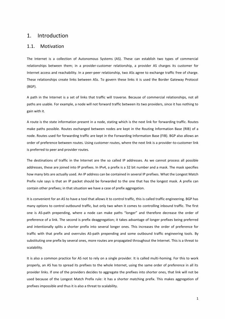
The Internet is a collection of Autonomous Systems (AS). These can establish two types of commercial
relationships between them; in a provider-customer relationship, a provider AS charges its customer for
Internet access and reachability. In a peer-peer relationship, two ASs agree to exchange traffic free of charge.
These relationships create links between ASs. To govern these links it is used the Border Gateway Protocol
(BGP).
A path in the Internet is a set of links that traffic will traverse. Because of commercial relationships, not all
paths are usable. For example, a node will not forward traffic between its two providers, since it has nothing to
gain with it.
A route is the state information present in a node, stating which is the next link for forwarding traffic. Routes
make paths possible. Routes exchanged between nodes are kept in the Routing Information Base (RIB) of a
node. Routes used for forwarding traffic are kept in the Forwarding Information Base (FIB). BGP also allows an
order of preference between routes. Using customer routes, where the next link is a provider-to-customer link
is preferred to peer and provider routes.
The destinations of traffic in the Internet are the so called IP addresses. As we cannot process all possible
addresses, these are joined into IP prefixes. In IPv4, a prefix is a 32 bit number and a mask. The mask specifies
how many bits are actually used. An IP address can be contained in several IP prefixes. What the Longest Match
Prefix rule says is that an IP packet should be forwarded to the one that has the longest mask. A prefix can
contain other prefixes; in that situation we have a case of prefix aggregation.
It is convenient for an AS to have a tool that allows it to control traffic, this is called traffic engineering. BGP has
many options to control outbound traffic, but only two when it comes to controlling inbound traffic. The first
one is AS-path prepending, where a node can make paths “longer” and therefore decrease the order of
preference of a link. The second is prefix deaggregation; it takes advantage of longer prefixes being preferred
and intentionally splits a shorter prefix into several longer ones. This increases the order of preference for
traffic with that prefix and overrules AS-path prepending and some outbound traffic engineering tools. By
substituting one prefix by several ones, more routes are propagated throughout the Internet. This is a threat to
scalability.
It is also a common practice for AS not to rely on a single provider. It is called multi-homing. For this to work
properly, an AS has to spread its prefixes to the whole Internet, using the same order of preference in all its
provider links. If one of the providers decides to aggregate the prefixes into shorter ones, that link will not be
used because of the Longest Match Prefix rule: it has a shorter matching prefix. This makes aggregation of
prefixes impossible and thus it is also a threat to scalability.
2
The Internet us routing system is facing serious scalability problems as it is widely recognized by the research
community[19]. The biggest one of them is the growth of forwarding and routing tables. This is caused
primarily by the Internet growth, increasing the number of IP prefixes as well as the growing use of
multihoming and traffic engineering.
Routing aggregation is the primary tool for increasing scalability in the Internet. We say routing aggregation is
done by merging specific prefixes into one aggregated one. If filtering is done afterwards, the specific prefixes
can be discarded therefore saving state information. There have been many attempts to address this. CIDR [20]
in 1993 relieved this issue temporarily, by the introduction of a new way of advertising prefixes. From then on,
the Internet use has been widespread to the world population and routing aggregation faced a more serious
challenge.
Draves et al [7] in 1998 proposed an optimal way of constructing IP forwarding tables, locally, that inspired
works like [16] and [30] who went a step further towards a practical implementation. The main idea behind
these works was to reduce the state information to its minimum, while maintaining the same output for every
IP destination. These were only meant to solve this problem in short term, since the architecture remained the
same and aggregation was done only in the Forward Information Base (FIB) of every node.
A different approach was taken by Jen et al [14] and Meyer with LISP[18]. These proposals try to solve the
problem of route aggregation by completely changing the architecture of the routing system. They aim to
separate the Internet into two sections, edges and core. Then, the IP addresses should also be separated into
two, a core and an edge address. This would result in huge savings in terms of state information, because a
node would only need the core address of distant nodes. However, a complete change like this is very difficult
to implement, like we have seen with IPv6.
Sobrinho and Le [25] have recently proposed the three aggregation strategies that we study. We can say that
no paths are changed if everyone participates. Also, this is not a short term solution, since it aggregates not
only FIB but also RIB and it is not only local. The changes in architecture are practically inexistent. Finally, to
address the problem of a transition period, we study partial participation.

3
1.2. Objectives
This work started as a deeper study of route aggregation of [25], but we thought it would be convenient to
study how the Internet can be described by inferred topologies in Chapter 2. We wanted to have a better
understanding of the input data that we were going to use to test the routing aggregation strategies. We used
inferred topologies by CAIDA[3] and UCLA[26], and looked at their data sources and inference algorithms.
Then, we found appropriate to study IPv4 prefix assignment in Chapter 3. We used the RouteViews data [27]
preprocessed by CAIDA [4]. Focusing on prefix aggregation in particular, we defined several metrics to help us
understand the status of the Internet us prefix tree. A similar study was done by Cittadini in [2], but centered
on prefix deaggregation.
Finally, in Chapter 4, we used the inferred network topologies to test routing aggregation strategies proposed
by Sobrinho and Le. We studied the most effective strategy, Implicit Long Routes for partial participation. This
was meant to understand what could be the consequences of a transitional period, where not every AS would
perform route aggregation.

4
5
2. Network Topologies
2.1. Basic Concepts
The Internet, as its name implies, is a set of many computer networks and their interconnections. Each one of
these smaller networks is called an Autonomous System (AS) because, unlike the Internet as a whole, its
management and operation are autonomous. An AS is ruled by only one entity. It has its unique AS number,
attributed by the Internet Assigned Numbers Authority (IANA). An AS can be, for example, an Internet Service
Provider (ISP) that provides transit traffic; a Content Provider or Content Distribution Network that mainly
hosts websites/services, or a large company or a university that pay their providers for Internet access. With so
many different ASs one can say that no one rules the Internet. Rather, it is ruled by everyone. Each AS will
make the decisions based on local commercial agreements that it establishes with neighbor domains. It will
choose the results that suits it best, rather than any defined common good.
There are two types of relationships that two neighbor ASs can establish. They can establish a customer-
provider agreement, where a customer AS pays a provider for Internet access. In this customer-provider
relationship, the provider is more likely to be on a higher level of the Internet’s hierarchy. This means it is
economically more powerful and thus exchanges more traffic. The other way two ASs can interconnect is
through a peering agreement. In this case, they agree to exchange traffic between them and their customers
with no financial settlements. In this case, both ASs will only benefit from the link if their dimension is similar;
meaning the traffic flowing on each direction of the link is approximately the same. These two forms of
connections were first modeled by Huston [12].
In order to test our AS-level routing solutions, we need a model that can depict these agreements and provide
a picture of the Internet as a whole. Our choice is obvious: a directed graph, G= (V, E). A graph is a
mathematical representation of a network, which means a set V of nodes and E links between those nodes.
Each link connects two nodes. Graphs can be used to represent any network, like biological, neural or social
networks. In the case of the Internet at AS level, we will model each AS as a node. Concerning the links, there
are two types of relationships that nodes (ASs) can establish, which means we will need to use a specific kind of
graph: an annotated graph. This is a graph where the links are labeled. Specifically, there can be peer-peer links
(p2p), customer-provider (c2p) links or provider-customer (p2c). Obviously, if two ASs are connected via a
customer-provider agreement, there is one c2p link and one p2c in opposite directions between them. A
sample AS-level network is shown in Figure 2.1.
6
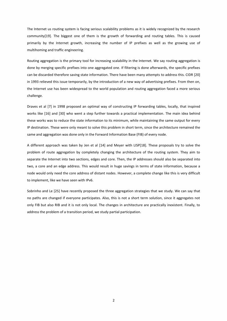
Figure 2.1 – A sample AS-level network
We can see that, for example, node A has a peering agreement with B and C. It also has two customers: D and
E. In every graph we place providers on top of their customers.
We say that a path in the Internet is a set of links that packets will traverse in order to reach a destination AS. A
route may be defined as information that is used to make a decision about how to forward a packet so that it
will reach its intended destination network. Not every path is usable. For a path to be usable, each node must
have the respective routes. A route can fall in three categories: customer, peer or provider, accordingly to the
next link (the neighbor from which it is learned). For example, if the link is a c2p link, then the route is a
provider route, since the next hop is a provider of the source node. The same applies to customer and peer
routes. The route export policies define which routes are to be advertised and which ones are not. An AS will
advertise every route that it learnt to its customers, since they are paying for Internet access. It will also
advertise all its customer routes to every neighbor. This is depicted on Table 2.1. Propagation of routes is in
the opposite direction of traffic flow.
Destination
Customers Peers Providers
Origin
Customer routes
Peer routes
Provider routes
Table 2.1 – IP routes export policies
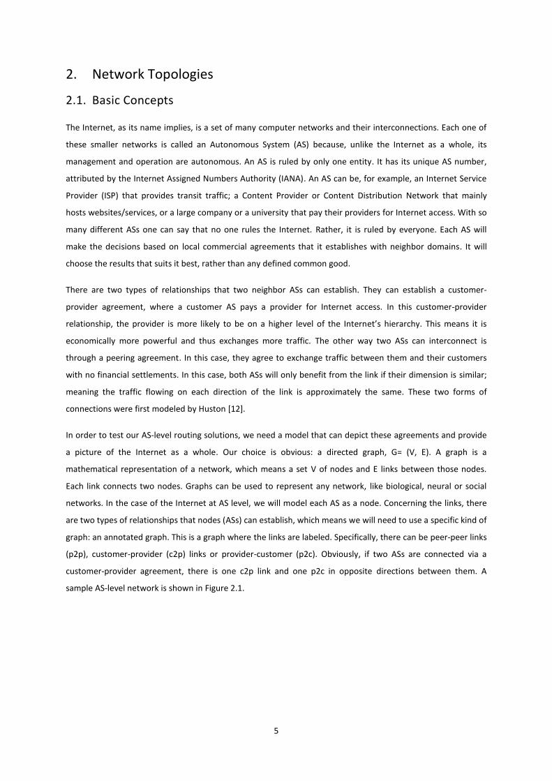
Over the Internet AS-level graph, paths are established between source and destination nodes. However, these
paths obey to specific rules, meaning they cannot traverse certain links due to routing export policies. The
resulting usable path must consist of a set of zero or more customer-to-provider links, followed by zero or one
peer-peer link, followed by zero or more provider-to-customer links. This is shown in Figure 2.2.
7
Figure 2.2 – Usable BGP paths
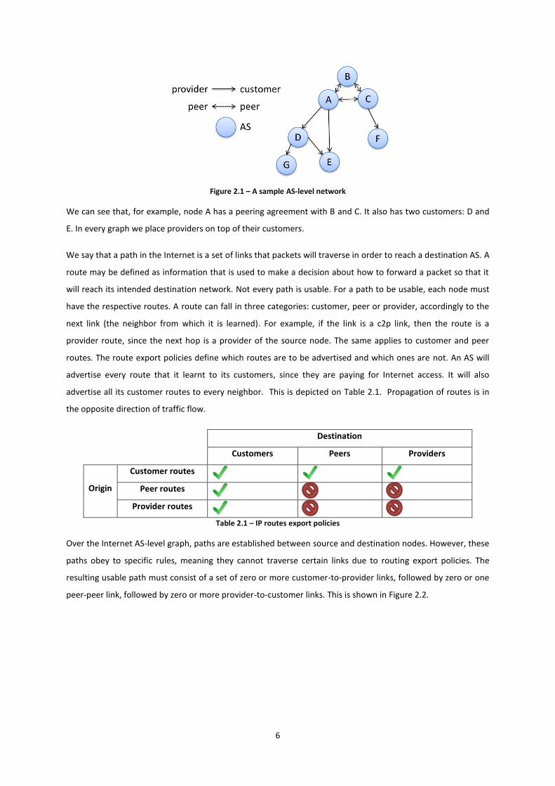
When we draw an AS graph, we are careful enough to place provider nodes on top of customer nodes. Then, all
the paths we obtain are valley-free. A valley is a path containing a p2c link before a c2p link. An example is
shown in Figure 2.3, where the path, in red, is forbidden because it has a valley in node E, i.e. D-E is a p2c link
and E-A is a p2c link. We will explore forbidden paths further in the next section.
Figure 2.3 – Forbidden and allowed path in an AS level graph
The usable paths can fall into three categories: customer paths, peer paths or provider paths. A customer path
is constituted only by p2c links, for example A-D-G. A peer path is constituted by a p2p link possibly followed by
c2p links, for example C-A-E. Finally, a provider path, like the one in the picture from G to F, is composed of one
or many c2p links possibly followed by a p2p and/or p2c links. We say that G is an indirect customer of A
because there is a customer path from A to G (via D). Symmetrically, A is an indirect provider of G.
How can we obtain a graph that resembles the Internet? BGP is the responsible protocol for exchanging routes
in the Internet. BGP routes can be collected and then processed in order to generate an inferred topology
graph. We chose to analyze graphs that are inferred from RouteViews’ BGP raw data (and other sources) by
CAIDA[3] or UCLA[26]. The construction of these graphs is made on the following manner: there are several
data sources, collecting information concerning traffic and route announcements. All this is gathered and a
certain algorithm infers a network topology from it. We will look carefully at this later. The other alternative is
to create a synthetic graph from scratch, which means designing an algorithm that we can input the total
number of nodes and then, it generates customer-provider and peer-peer links between those nodes, like [8] .
We must set some metrics to understand what characteristics each graph has. In the case of AS level topology,
we can measure degree distribution. We can also breakdown degree distribution into customer, provider and
peer distribution. We say that the degree of a node is the number of neighbors it has. These statistical
distributions help us understand how AS interact with each other. It is generally accepted by the literature [9]
8
and [28] that ASs with a high degree are the ones that are more economically powerful and have larger
operations. So node degree distribution can help us establish an AS hierarchy.
Well, but is degree distribution enough? Can we think of something else even better to organize nodes in a
hierarchy? The answer is to classify each node with a number and call it tier. The tier of an AS is a very
important characteristic. Tier 1 nodes are AS that do not have providers, this means that they do not pay
anyone for Internet connectivity, but they must ensure it to all their customers. This requirement makes it very
difficult for an AS to be on tier-1 and consequently only a few are economical capable of it, we found 13. There
is a consensus about the definition of tier-1 ASs in the literature. The same is not true for tier n, with n>1 and
that is why we used the following definition: a tier of an AS is the minimum tier of its providers +1. This
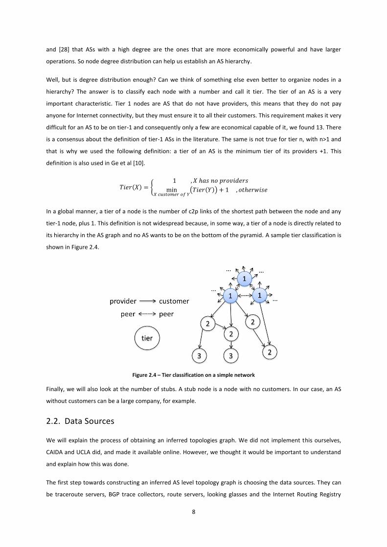
definition is also used in Ge et al [10].
( ) {
( ( ))
In a global manner, a tier of a node is the number of c2p links of the shortest path between the node and any
tier-1 node, plus 1. This definition is not widespread because, in some way, a tier of a node is directly related to
its hierarchy in the AS graph and no AS wants to be on the bottom of the pyramid. A sample tier classification is
shown in Figure 2.4.
Figure 2.4 – Tier classification on a simple network
Finally, we will also look at the number of stubs. A stub node is a node with no customers. In our case, an AS
without customers can be a large company, for example.
2.2. Data Sources
We will explain the process of obtaining an inferred topologies graph. We did not implement this ourselves,
CAIDA and UCLA did, and made it available online. However, we thought it would be important to understand
and explain how this was done.
The first step towards constructing an inferred AS level topology graph is choosing the data sources. They can
be traceroute servers, BGP trace collectors, route servers, looking glasses and the Internet Routing Registry
9
(IRR) databases, according to Zhang et al[29]. These must provide to the inference algorithms a list of paths, or
simply pairs of connected ASs. Let us look at each one carefully.
A traceroute server is simply a computer that uses the traceroute tool to send packets to a given IP address as
destination, with an increasing number as a limit for hop counts. It receives an ICMP message originated by the
last router to receive the packet. The route of the packet is derived from that. The last step is to convert router
IP addresses into AS numbers.
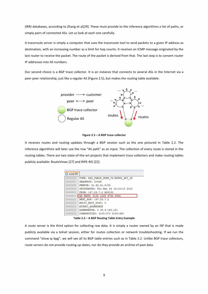
Our second choice is a BGP trace collector. It is an instance that connects to several ASs in the Internet via a
peer-peer relationship, just like a regular AS (Figure 2.5), but makes the routing table available.
Figure 2.5 – A BGP trace collector
It receives routes and routing updates through a BGP session such as the one pictured in Table 2.2. The
inference algorithms will later use the row “AS path” as an input. The collection of every route is stored in the
routing tables. There are two state-of-the-art projects that implement trace collectors and make routing tables
publicly available: RouteViews [27] and RIPE-RIS [22].
Table 2.2 – A BGP Routing Table Entry Example
A route server is the third option for collecting raw data. It is simply a router owned by an ISP that is made
publicly available via a telnet session, either for routes collection or network troubleshooting. If we run the
command “show ip bpg”, we will see all its BGP table entries such as in Table 2.2. Unlike BGP trace collectors,
route servers do not provide routing up-dates, nor do they provide an archive of past data.

10
A looking glass is the fourth option, it is also a server belonging to an ISP but it features a web interface that
allows us to run a limited set of commands. Although it does not show us the full BGP table, including the “AS
paths” we wanted, it is able to display the router’s direct neighbors by running “show ip bgp summary”.
Finally, there are the Internet Routing Registry (IRR) databases. These do not belong to a particular ISP. Instead,
they are kept by several ISPs on a voluntary basis in order to coordinate routing policies. Each AS will have an
entry on this registry stating which routes it imports and exports to each one of its direct neighbors. As these
registries in Europe are of mandatory update by ISPs, we can say that those are the most reliable sources.
Figure 2.6 - RIPE IRR example for Vodafone in Portugal, ASN column shows the neighbors, Power is their degree
UCLA updates (and makes available) its dataset daily using BGP trace collectors (Route Views, RIPE-RIS,
Abilene), route servers (Packet Clearing House, UCR, traceroute.org, Route Server Wiki), looking glasses
(traceroute.org, NANOG, Looking Glass Wiki) and a portion of RIPE IRR, which is a larger set of policy paths
inputs than CAIDA that only uses RouteViews.
CAIDA has two main datasets, the first one is called “Topology: Macroscopic Internet Topology Data Kit (Ark
ITDK)” and it is the state-of-the-art traceroute-based topology. There is, however, a difficulty as for assigning
AS numbers to IP prefixes and therefore this dataset does not work as an AS-level graph. The second dataset is
merely called “AS Relationships” and is only based in RouteViews data. This is what we will use and call CAIDA
dataset in the remaining of this work. Also, this is not updated on a daily basis and so we will use the January
2011 graph, which is the most recent one.
The data sources’ general characteristics are summarized in Table 2.3.

11
Data Source Projects Output Used by CAIDA Used by UCLA
Traceroute Server traceroute.org Paths (with no
AS numbers)
No No
BGP Trace Collector RouteViews, RIPE-RIS Paths Only
RouteViews
Yes
Route Server Packet Clearing House, UCR,
traceroute.org, Route Server Wiki
Paths No Yes
Looking Glass traceroute.org, NANOG, Looking Glass
Wiki
Neighbors list No Yes
Internet Routing Registry RIPE portion Neighbors list No Yes
Table 2.3 - Summary of inferred topologies' data sources
2.3. Inference Algorithms
The second (and last) step to building an AS graph based on measurements is to develop an inference
algorithm. These algorithms use paths as inputs and produce annotated graphs. These paths are from BGP
routing tables and are present in the AS-PATH attribute. In the case of looking glasses and the Internet Routing
Registry these are only links (or paths with 1 hop) since they only provide a set of neighbors per AS. The main
idea behind inference algorithms is shown in Figure 2.7: A node’s economic power/hierarchy level is measured
by its degree (the number of neighbors). If a node X connects to a node Y, the choice for the link to be p2p, c2p
or p2c is based on X’s and Y’s degrees (Figure 2.7).
Figure 2.7 – Inferring logical relationships from the routing table entries
The inference algorithm used by CAIDA is described by Dimitropoulos in [6] and is based on the work of Gao[9].
The algorithm is formulated as an optimization problem of two constrains. The first one is to adjust the
customer-provider and peer-peer relationships accordingly to each node’s degree. For example, let us say that
the following path was observed: A(5)-B(50)-C(2000)-D(1900) where the numbers in parenthesis represent
each node’s degree. Just taking this constrain into account, A must be a customer of B because A’s degree is
lower. The same applies to B-C. On the other hand, the link C-D is inferred as peer-to-peer because both ASs
degrees have the same order of magnitude. This is basically the inference algorithm proposed by Gao[9]. Now,
the second constrain is to maximize the number of usable paths. The simplest way to understand this is with
another example: we observe the path X(5)-Y(6)-Z(100). By adjusting node’s degree to relationships we simply
12
say X and Y are peers and Z provides Y. The problem is that this is not a valid path, since after a peer-peer link,
packets shall only pass provider-customer links, and not customer-provider as we inferred. In short, this
algorithm relies on the tradeoff between using valid paths and assigning c2p links according to node’s degree.
Using the true relationships of 3,724 links, provided by some ISPs that gave the authors of [6] their lists of
neighbor ASs, they confirmed that these heuristics achieved very high accuracy of 96.5% (c2p) and 82.8% (p2p)
of correctly inferred relationships, with the overall accuracy being 94.2%. This algorithm associated to BGP
trace collectors is known for underestimating p2p links, since trace collectors are more focused on routes that
reach the core of the Internet. This happens because they have a limited number of peering ASs, namely core
ISPs. That is one of the reasons why UCLA implemented their own topology dataset with more data sources.
The Inference algorithm used by UCLA is described in [17] and also based on the work of Gao [9]. This time, it
starts by assuming (as we did) that the Internet AS-level graph has its core in a set of tier-1 nodes that
interconnect via peering relationships. The authors use the list in Wikipedia [28] to collect their AS numbers.
Now, every AS must be a direct/indirect customer of at least one of these tier-1 nodes. Assuming this, they look
at input paths, which are gathered using the data sources described above, that include every tier-1 AS BGP
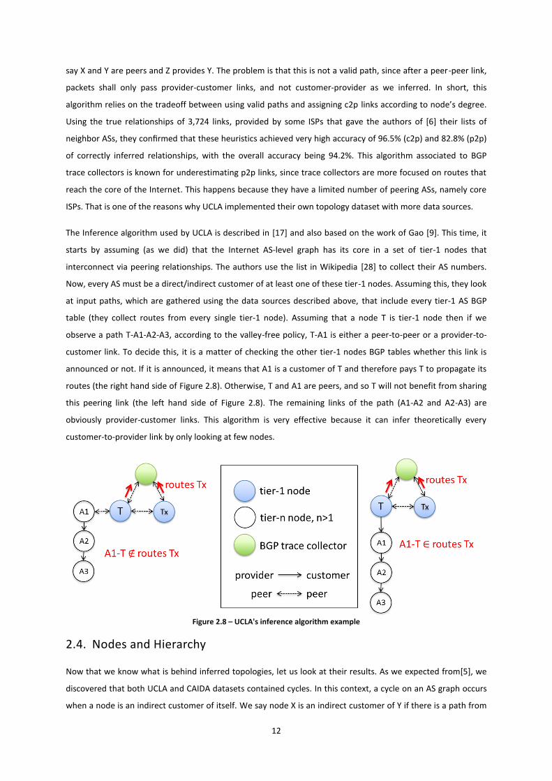
table (they collect routes from every single tier-1 node). Assuming that a node T is tier-1 node then if we
observe a path T-A1-A2-A3, according to the valley-free policy, T-A1 is either a peer-to-peer or a provider-to-
customer link. To decide this, it is a matter of checking the other tier-1 nodes BGP tables whether this link is
announced or not. If it is announced, it means that A1 is a customer of T and therefore pays T to propagate its
routes (the right hand side of Figure 2.8). Otherwise, T and A1 are peers, and so T will not benefit from sharing
this peering link (the left hand side of Figure 2.8). The remaining links of the path (A1-A2 and A2-A3) are
obviously provider-customer links. This algorithm is very effective because it can infer theoretically every
customer-to-provider link by only looking at few nodes.
Figure 2.8 – UCLA's inference algorithm example
2.4. Nodes and Hierarchy
Now that we know what is behind inferred topologies, let us look at their results. As we expected from[5], we
discovered that both UCLA and CAIDA datasets contained cycles. In this context, a cycle on an AS graph occurs
when a node is an indirect customer of itself. We say node X is an indirect customer of Y if there is a path from

13
X to Y containing only provider-to-customer links (at least 2). In this case, if AS X is customer of AS Y, Y is
customer of Z and Z is a customer of X, then there is a cycle because X, Y and Z are indirect customers of
themselves. In the route aggregation algorithms that we will study, we do not deal with cycles and thus they
have to be removed a priori. On the other hand, cycles in the Internet may not allow some packets to reach
their destinations, making them loop and eventually be discarded. Cycles can be a consequence of reading in
different instants of time, or nodes can provide other nodes for only certain prefixes or regions of the globe. In
order to detect cycles in a graph we used a depth-first-search algorithm (DFS).
The following concern is how to remove that cycle, which link should we break: X->Y, Y->Z or Z->X? First, we
tried to choose the link in which the provider has the lowest tier and break it. For example, if tier(X)=3,
tier(Y)=4 and tier(Z)=2 then we will break link Y->Z since it is not very likely that a tier-4 AS is a provider of a
tier-2. This had one downside, it made us reset the DFS search every time a cycle was found. To avoid it, we
chose to break the last link seen in the cycle. Then the DFS could continue without the need to reset. This
proved to reduce by a factor of 10 the amount of time necessary to run the algorithm. The results, in particular
tier distribution of the network and the connectivity of the nodes in the cycles were not much affected. We
removed 321 links from CAIDA dataset and 213 from UCLA.
Let us address the problem of policy-connectivity. We define a graph to be policy-connected if there is a valley-
free path between every possible pair of nodes. In our case, we assume that tier-1 one nodes are able to reach
every node that is in the Internet. So, we define as policy-disconnected ASs those nodes that cannot reach tier-
1 nodes (or the Internet core). We found that situation in both UCLA and CAIDA datasets. This would mean that
some nodes could not reach the Internet core according to the customer-provider/peer-peer relationships and
export policies that we established. So, we have to address this problem. As we have explained earlier, paths in
the AS graph are “valley free”, which makes certain restrictions in which links are eligible for packets to go from
one source to a destination. It can happen that despite a node being connected to the graph through one or
many links, it cannot reach most of the other nodes because of export policies. The algorithm to detect and
remove these nodes is also very simple.
First, we classify as tier-1 every node that is in the tier-1 network node list in Wikipedia[28], Table 2.4. We did
not include AOL because it is allegedly paying for peering settlements and AS number 1 from Level-3 because it
had several providers. This resulted in a total of 13 nodes. We used this list because our previous definition of
tier-1 nodes, in Figure 2.4, showed us approximately 40 nodes as tier-1 ASs. This was caused by reading errors
in the inferred topologies. This list in Wikipedia is generally accepted by the literature [17] and therefore, it is a
more reliable source.
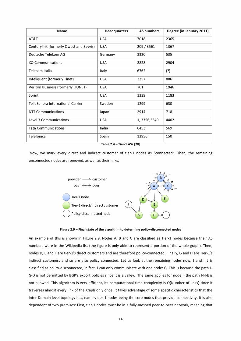
14
Name Headquarters AS numbers Degree (in January 2011)
AT&T USA 7018 2365
Centurylink (formerly Qwest and Savvis) USA 209 / 3561 1367
Deutsche Telekom AG Germany 3320 535
XO Communications USA 2828 2904
Telecom Italia Italy 6762 (?)
Inteliquent (formerly Tinet) USA 3257 886
Verizon Business (formerly UUNET) USA 701 1946
Sprint USA 1239 1183
TeliaSonera International Carrier Sweden 1299 630
NTT Communications Japan 2914 718
Level 3 Communications USA 1, 3356,3549 4402
Tata Communications India 6453 569
Telefonica Spain 12956 150
Table 2.4 – Tier-1 ASs [28]
Now, we mark every direct and indirect customer of tier-1 nodes as “connected”. Then, the remaining
unconnected nodes are removed, as well as their links.
Figure 2.9 – Final state of the algorithm to determine policy-disconnected nodes
An example of this is shown in Figure 2.9. Nodes A, B and C are classified as Tier-1 nodes because their AS
numbers were in the Wikipedia list (the figure is only able to represent a portion of the whole graph). Then,
nodes D, E and F are tier-1’s direct customers and are therefore policy-connected. Finally, G and H are Tier-1’s
indirect customers and so are also policy connected. Let us look at the remaining nodes now, J and I. J is
classified as policy-disconnected, in fact, J can only communicate with one node: G. This is because the path J-
G-D is not permitted by BGP’s export policies since it is a valley. The same applies for node I, the path I-H-E is
not allowed. This algorithm is very efficient, its computational time complexity is O(Number of links) since it
traverses almost every link of the graph only once. It takes advantage of some specific characteristics that the
Inter-Domain level topology has, namely tier-1 nodes being the core nodes that provide connectivity. It is also
dependent of two premises: First, tier-1 nodes must be in a fully-meshed peer-to-peer network, meaning that

15
between every possible pair of tier-1 nodes there is a p2p link. Second, the connected part of the network is
the one that contains every tier-1 direct/indirect customer.
We removed 847 nodes for UCLA and 1452 for CAIDA dataset. Despite being a reasonably amount of lost
information, we believe that it is more important to work with a policy-strongly-connected graph[25]. This
means there is a path respecting BGP’s export policies between every pair of nodes, namely valley-free paths.
To finish this section, we present the results after processing the datasets as explained earlier. First, let us focus
on Table 2.5.
Table 2.5 – Statistical comparison between CAIDA and UCLA datasets
We can see that being a tier-1 node does not necessarily mean that one has no providers. This may be
explained by the fact that nodes can be economically powerful in one region of the globe, but in other regions
they have to pay their providers. On the other hand, all these measures are imperfect and there is always the
possibility of errors.
It is quite clear that the tier-1 nodes were chosen correctly, since their average degree is over 1000. Being
connected to one of these nodes is equivalent to reaching everyone in the Internet. We also said that tier-1
nodes were in a fully meshed peering graph. Looking at the data, from the possible 12×13=156 peering links,
UCLA captured all 156 and CAIDA captured 154, which clearly corroborates our assumption.
The number of tiers is very important as well. Observing 6 tiers means that, in the worst case scenario, a node
needs 6 hops to reach a tier-1 AS. We believe this number is accurate and asserts that this structure for the AS-
level topology assures scalability.
The average number of customers, peers and providers that an ASs connects is decreasing with the increasing
tier, which suggests that the tier of a node and its degree are two concordant ways to classify nodes into a
hierarchy.
Now, let us compare UCLA with CAIDA dataset. As we mentioned earlier, UCLA uses a wider range of data
sources. This is the cause for the observation of more links that are unseen by RouteViews (CAIDA’s only data
source). Figure 2.10 shows that.
Tier
CAIDA UCLA CAIDA UCLA CAIDA UCLA CAIDA UCLA CAIDA UCLA CAIDA UCLA
1 13 13 0 0 1257,5 1302,1 1137,6 1136,6 0,2 0,0 119,7 165,5
2 10415 10510 7925 7969 12,7 15,9 3,8 3,7 2,6 2,6 6,4 9,6
3 21208 21515 18160 18441 3,7 4,2 0,9 0,9 1,8 1,8 0,9 1,5
4 6220 6616 5672 6030 2,0 2,3 0,2 0,2 1,3 1,3 0,4 0,7
5 453 519 424 477 1,8 2,4 0,3 0,3 1,2 1,1 0,4 1,0
6 68 83 67 81 2,7 1,2 0,0 0,0 1,0 1,0 1,6 0,2
Overall 38377 39256 32248 32998 6,3 7,5 1,9 1,9 1,9 1,9 2,3 3,6
Nodes Average Degree Avg #Customers Avg #Providers Avg #PeersStubs

16
Figure 2.10 – Node degree distributions
The ‘+’ signs referring to the UCLA dataset are slightly to the right of the ‘x’ signs (CAIDA). This indicates a
higher degree, meaning more links, are observed by UCLA’s data sources.
To assert the importance of tier-1 nodes, we wanted to see how many paths in the Internet contained these
nodes. For this, we calculated the paths between every pair of nodes according to the following BGP rules:
- A customer path is preferred to peer or provider paths.
- A peer path is preferred to provider paths.
- If there are several paths with the same type, we chose the one with less hops (the shortest length).
- If there are several paths with the same type and equal length, we chose one at random.
Figure 2.11 - BGP path choice
Using these rules, we modified Dijkstra’s algorithm to use it to calculate BGP paths. The modification was done
by replacing the arithmetic sum of distances by a BGP sum matrix, Table 2.6, in which we sum paths to links.
This table is the result of BGP export policies, in Table 2.1.
2nd
term (link)
c2p p2p p2c
1st
term (path)
Customer/Null Customer path Peer path Provider path
Peer Provider path Invalid path
Provider Provider path
Table 2.6 – Dijkstra's algorithm's sum of a path and a link
100
101
102
103
104
100
101
102
103
104
105
Node degree
Fre
quency
CAIDA
UCLA
Number

17
After waiting 4 hours, we reached the conclusion that 53.1% of all paths contained a tier-1 node. This number
is very high, since tier-1 nodes are only 13 in a universe of approximately 40000.
To assert this fact, we performed another experiment. We removed all tier-1 nodes from our graph.
Consequently, the graph was no longer policy-connected and some nodes could not communicate with others
using BGP valid paths. We calculated again the paths between every pair of nodes according to the same BGP
rules. On average, a node could not reach 15.6% of the remaining ASs. It corroborates the idea that tier-1
nodes have tremendous power.

18
19
3. Prefix to AS Mappings
3.1. Introduction
In this section we will analyze the prefix to AS mappings in the Internet. These mappings are set of prefixes that
are announced and their corresponding AS (the AS that is the destination for a packet with that prefix). We will
look to this data aiming to understand what the current status of the prefix distribution is. We have developed
a set of metrics to help us process this data. We will present them, their algorithms for calculation and final
results.
3.2. Data Source
To start, let us understand where this data comes from, and how is it processed into a single output file. For
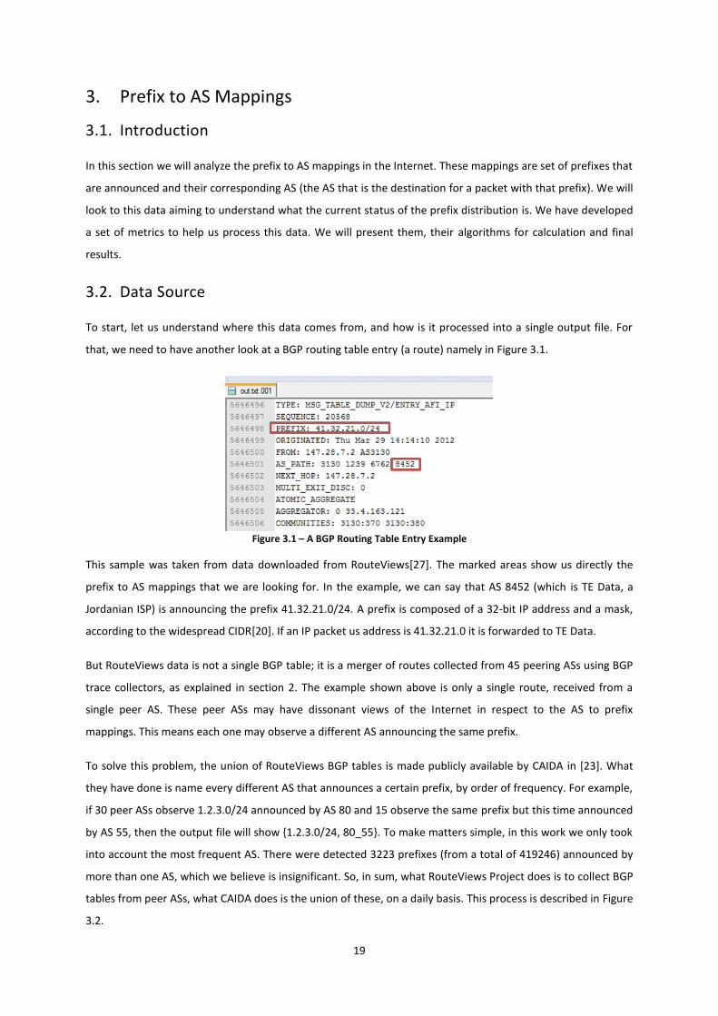
that, we need to have another look at a BGP routing table entry (a route) namely in Figure 3.1.
Figure 3.1 – A BGP Routing Table Entry Example
This sample was taken from data downloaded from RouteViews[27]. The marked areas show us directly the
prefix to AS mappings that we are looking for. In the example, we can say that AS 8452 (which is TE Data, a
Jordanian ISP) is announcing the prefix 41.32.21.0/24. A prefix is composed of a 32-bit IP address and a mask,
according to the widespread CIDR[20]. If an IP packet us address is 41.32.21.0 it is forwarded to TE Data.
But RouteViews data is not a single BGP table; it is a merger of routes collected from 45 peering ASs using BGP
trace collectors, as explained in section 2. The example shown above is only a single route, received from a
single peer AS. These peer ASs may have dissonant views of the Internet in respect to the AS to prefix
mappings. This means each one may observe a different AS announcing the same prefix.
To solve this problem, the union of RouteViews BGP tables is made publicly available by CAIDA in [23]. What
they have done is name every different AS that announces a certain prefix, by order of frequency. For example,
if 30 peer ASs observe 1.2.3.0/24 announced by AS 80 and 15 observe the same prefix but this time announced
by AS 55, then the output file will show {1.2.3.0/24, 80_55}. To make matters simple, in this work we only took
into account the most frequent AS. There were detected 3223 prefixes (from a total of 419246) announced by
more than one AS, which we believe is insignificant. So, in sum, what RouteViews Project does is to collect BGP
tables from peer ASs, what CAIDA does is the union of these, on a daily basis. This process is described in Figure
3.2.
20
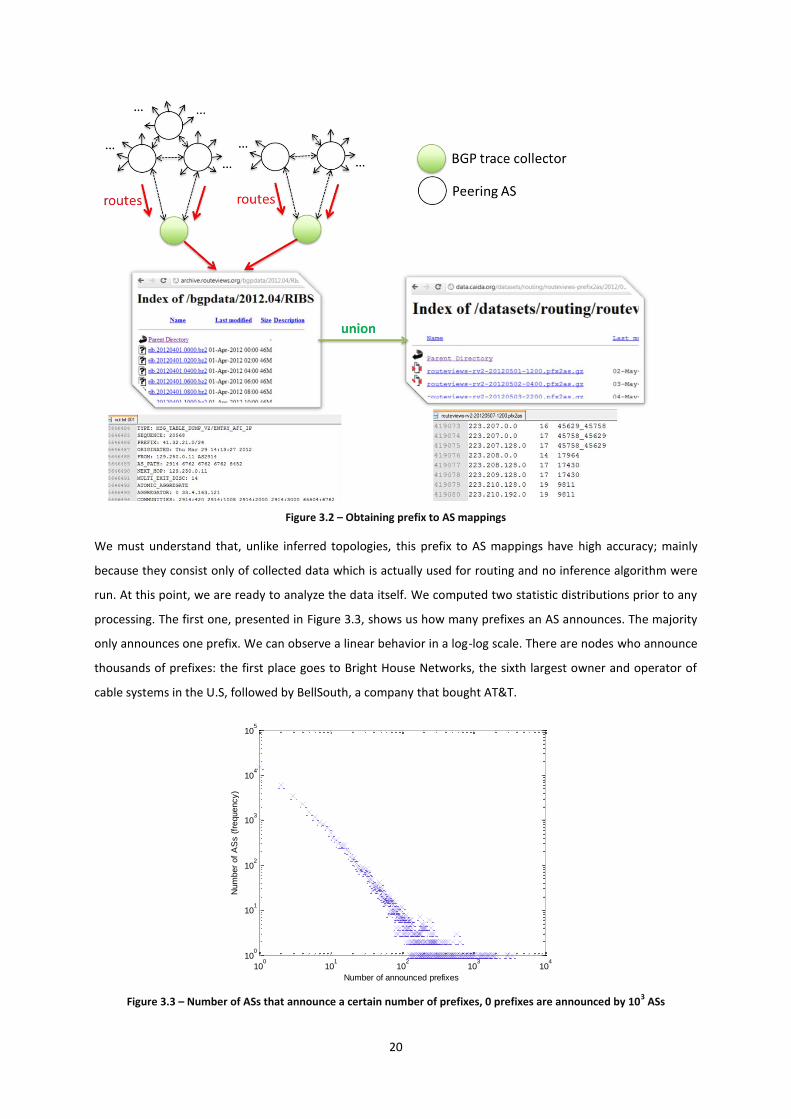
Figure 3.2 – Obtaining prefix to AS mappings
We must understand that, unlike inferred topologies, this prefix to AS mappings have high accuracy; mainly
because they consist only of collected data which is actually used for routing and no inference algorithm were
run. At this point, we are ready to analyze the data itself. We computed two statistic distributions prior to any
processing. The first one, presented in Figure 3.3, shows us how many prefixes an AS announces. The majority
only announces one prefix. We can observe a linear behavior in a log-log scale. There are nodes who announce
thousands of prefixes: the first place goes to Bright House Networks, the sixth largest owner and operator of
cable systems in the U.S, followed by BellSouth, a company that bought AT&T.
Figure 3.3 – Number of ASs that announce a certain number of prefixes, 0 prefixes are announced by 103 ASs
100
101
102
103
104
100
101
102
103
104
105
Number of announced prefixes
Num
ber
of
AS
s (
frequency)

21
The second statistical distribution was meant to tell us what the mask distribution in the Internet is. For
example, if there are more announced prefixes /24 or /23. This is shown in Figure 3.4, on the left side. On the
right side, we computed the same variable (number of prefixes) but divided by its maximum possible. For
example, the number of /16 prefixes was divided by 2^16 and multiplied by 100%.
Figure 3.4 – Mask size distribution
The conclusion is drawn after a glance, the most announced prefixes in the Internet are /24, which is actually
the maximum allowed. The minimum allowed mask is 8 bits. Concerning the normalized values, on the right,
we see that /16 prefixes are the ones that are mostly used (19%), when compared to its maximum.
3.3. Prefix Tree Construction
As we said earlier, the prefix mappings consist of 419246 prefixes and their corresponding ASs, this means that
the algorithms that we will use with this input data must be efficient. On the other hand, data is collected from
real-life routers, but we are only looking for Inter-domain data. So, we must eliminate all private prefixes.
According to [21] these prefixes are within the 10.0.0.0/8, 172.16.0.0/12 or 192.168.0.0/16 ranges. In addition
to this, it was also required to eliminate all prefixes whose mask is above 24 bits. This is because in the Inter-
domain level, these prefixes cannot be advertised [20] and consequently they belong to routers within the
same AS. Overall, the eliminated prefixes were 4168 (1%).
We need to choose a data structure to store the prefixes. We picked a binary tree, because it would take
advantage of the bitwise nature of Internet us prefixes. A tree node is a prefix. Each prefix can have zero, one
or two children. Thus, it is not a balanced tree. Prefixes always have one father, except for the root. The root of
the tree is the prefix 0.0.0.0/0. Its children are 0.0.0.0/1 and 128.0.0.0/1. The conversion to binary is
128(10)=1000 0000(2). More generally, each prefix can have two children: 0 and 1. This states which bit is to be
added to the original prefix. To make matters simple let us look at a sample tree in Figure 3.5.
8 10 12 14 16 18 20 22 2410
1
102
103
104
105
106
Num
ber
of
Pre
fixes (
frequency)
Mask size [bits]
8 10 12 14 16 18 20 22 240
2
4
6
8
10
12
14
16
18
20
Perc
enta
ge o
f pre
fixes /
x u
sed f
rom
all
/x p
ossib
le
Mask size [bits]
22
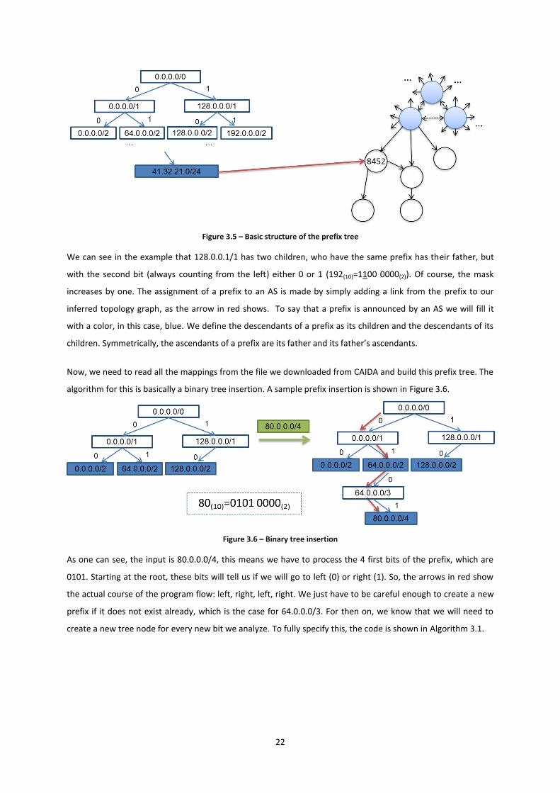
Figure 3.5 – Basic structure of the prefix tree
We can see in the example that 128.0.0.1/1 has two children, who have the same prefix has their father, but
with the second bit (always counting from the left) either 0 or 1 (192(10)=1100 0000(2)). Of course, the mask
increases by one. The assignment of a prefix to an AS is made by simply adding a link from the prefix to our
inferred topology graph, as the arrow in red shows. To say that a prefix is announced by an AS we will fill it
with a color, in this case, blue. We define the descendants of a prefix as its children and the descendants of its
children. Symmetrically, the ascendants of a prefix are its father and its father’s ascendants.
Now, we need to read all the mappings from the file we downloaded from CAIDA and build this prefix tree. The
algorithm for this is basically a binary tree insertion. A sample prefix insertion is shown in Figure 3.6.
Figure 3.6 – Binary tree insertion
As one can see, the input is 80.0.0.0/4, this means we have to process the 4 first bits of the prefix, which are
0101. Starting at the root, these bits will tell us if we will go to left (0) or right (1). So, the arrows in red show
the actual course of the program flow: left, right, left, right. We just have to be careful enough to create a new
prefix if it does not exist already, which is the case for 64.0.0.0/3. For then on, we know that we will need to
create a new tree node for every new bit we analyze. To fully specify this, the code is shown in Algorithm 3.1.
23
//Data structure for a tree node typedef struct prefix{ PREFIX* father; PREFIX* child[2]; AS* as; int level; int mask; } PREFIX //tree insertion void insert(PREFIX* root, AS* as, int* ip, int mask){
int i , bit, construction_mode=0;
PREFIX* p = root;
for (i = 0;i < mask;i++ ){
bit = (ip >> (31–i)) & 1;
if (p->child[bit] == NULL)
construction_mode = 1;
if (construction_mode)
p->child[bit] = new_prefix();
p = p->child[bit];
}
p->as = as;
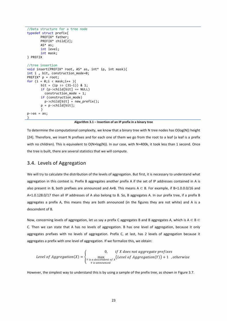
} Algorithm 3.1 – Insertion of an IP prefix in a binary tree
To determine the computational complexity, we know that a binary tree with N tree nodes has O(log(N)) height
[24]. Therefore, we insert N prefixes and for each one of them we go from the root to a leaf (a leaf is a prefix
with no children). This is equivalent to O(N×log(N)). In our case, with N≈400k, it took less than 1 second. Once
the tree is built, there are several statistics that we will compute.
3.4. Levels of Aggregation
We will try to calculate the distribution of the levels of aggregation. But first, it is necessary to understand what
aggregation in this context is. Prefix B aggregates another prefix A if the set of IP addresses contained in A is
also present in B, both prefixes are announced and A≠B. This means A ⊂ B. For example, if B=1.0.0.0/16 and
A=1.0.128.0/17 then all IP addresses of A also belong to B. So, B aggregates A. In our prefix tree, if a prefix B
aggregates a prefix A, this means they are both announced (in the figures they are not white) and A is a
descendent of B.
Now, concerning levels of aggregation, let us say a prefix C aggregates B and B aggregates A, which is A ⊂ B ⊂
C. Then we can state that A has no levels of aggregation. B has one level of aggregation, because it only
aggregates prefixes with no levels of aggregation. Prefix C, at last, has 2 levels of aggregation because it
aggregates a prefix with one level of aggregation. If we formalize this, we obtain:
( ) {
( ( ))
However, the simplest way to understand this is by using a sample of the prefix tree, as shown in Figure 3.7.
24
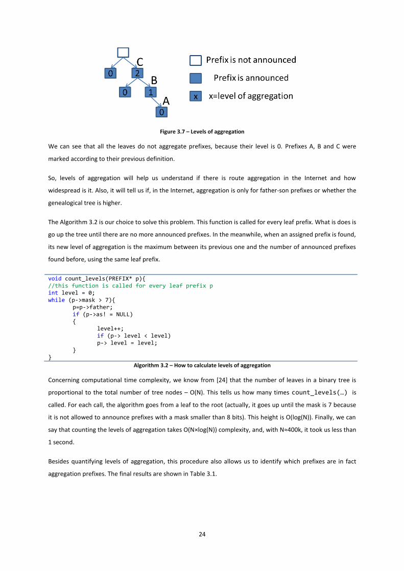
Figure 3.7 – Levels of aggregation
We can see that all the leaves do not aggregate prefixes, because their level is 0. Prefixes A, B and C were
marked according to their previous definition.
So, levels of aggregation will help us understand if there is route aggregation in the Internet and how
widespread is it. Also, it will tell us if, in the Internet, aggregation is only for father-son prefixes or whether the
genealogical tree is higher.
The Algorithm 3.2 is our choice to solve this problem. This function is called for every leaf prefix. What is does is
go up the tree until there are no more announced prefixes. In the meanwhile, when an assigned prefix is found,
its new level of aggregation is the maximum between its previous one and the number of announced prefixes
found before, using the same leaf prefix.
void count_levels(PREFIX* p){ //this function is called for every leaf prefix p
int level = 0;
while (p->mask > 7){
p=p->father;
if (p->as! = NULL)
{
level++;
if (p-> level < level)
p-> level = level;
}
} Algorithm 3.2 – How to calculate levels of aggregation
Concerning computational time complexity, we know from [24] that the number of leaves in a binary tree is
proportional to the total number of tree nodes – O(N). This tells us how many times count_levels(…) is
called. For each call, the algorithm goes from a leaf to the root (actually, it goes up until the mask is 7 because
it is not allowed to announce prefixes with a mask smaller than 8 bits). This height is O(log(N)). Finally, we can
say that counting the levels of aggregation takes O(N×log(N)) complexity, and, with N≈400k, it took us less than
1 second.
Besides quantifying levels of aggregation, this procedure also allows us to identify which prefixes are in fact
aggregation prefixes. The final results are shown in Table 3.1.
25
Level of Aggregation Number of prefixes
0 369485
1 32264
2 5222
3 973
4 201
5 38
6 11
7 2
Σ = 408196
Table 3.1 – Levels of aggregation
The vast majority of the prefixes in the Internet are leaves (369485). This means they do not play a role in route
aggregation. The remaining ones contain IP addresses that are also contained in other prefixes. We can see
that in the worst case scenario a prefix can be aggregated 7 times. So, real-life aggregation algorithms must
accommodate this hierarchy and not only model prefixes as father-son. The two 7-times aggregated prefixes
belong to CRNet - China Railways Network and to AirBand Communications, an American ISP.
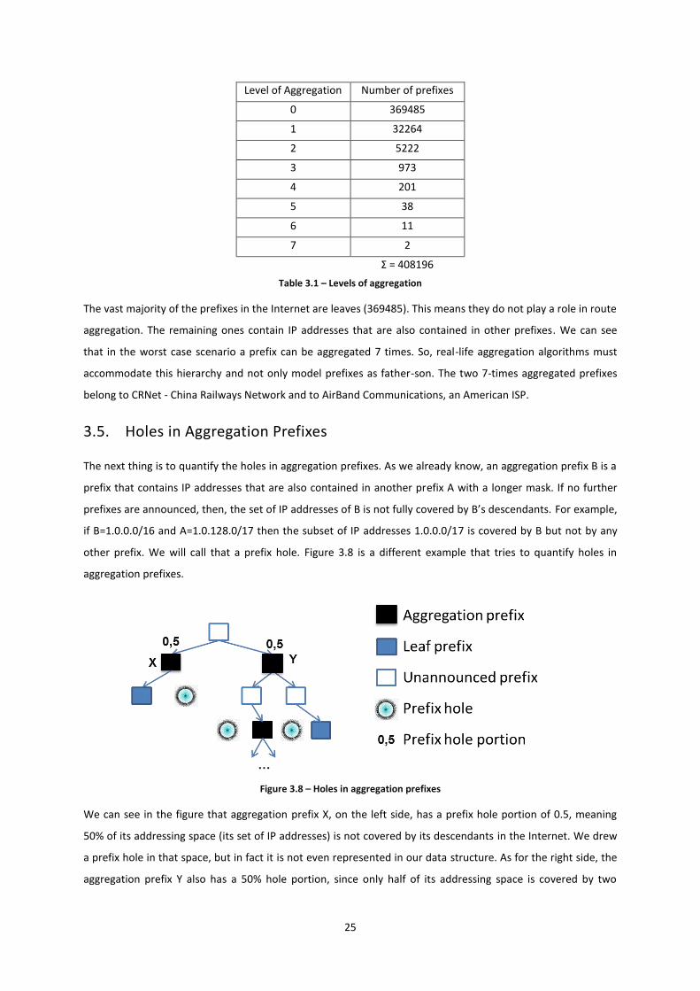
3.5. Holes in Aggregation Prefixes
The next thing is to quantify the holes in aggregation prefixes. As we already know, an aggregation prefix B is a
prefix that contains IP addresses that are also contained in another prefix A with a longer mask. If no further
prefixes are announced, then, the set of IP addresses of B is not fully covered by B’s descendants. For example,
if B=1.0.0.0/16 and A=1.0.128.0/17 then the subset of IP addresses 1.0.0.0/17 is covered by B but not by any
other prefix. We will call that a prefix hole. Figure 3.8 is a different example that tries to quantify holes in
aggregation prefixes.
Figure 3.8 – Holes in aggregation prefixes
We can see in the figure that aggregation prefix X, on the left side, has a prefix hole portion of 0.5, meaning
50% of its addressing space (its set of IP addresses) is not covered by its descendants in the Internet. We drew
a prefix hole in that space, but in fact it is not even represented in our data structure. As for the right side, the
aggregation prefix Y also has a 50% hole portion, since only half of its addressing space is covered by two
26
grandchildren. If not properly handled, these prefix holes can generate black holes, which attract and discard
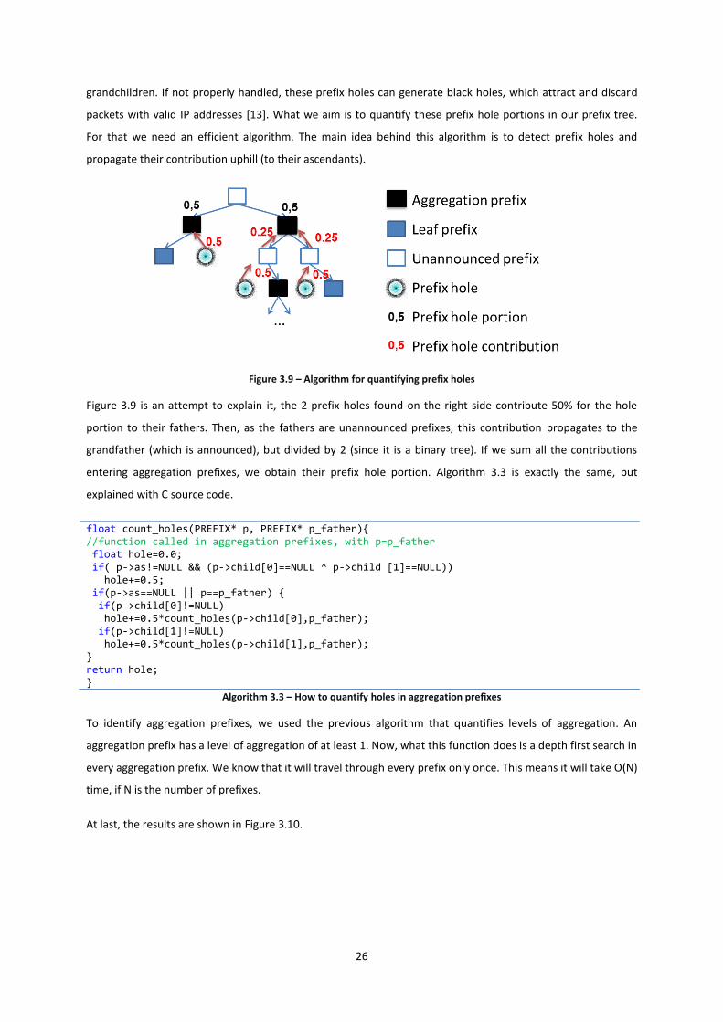
packets with valid IP addresses [13]. What we aim is to quantify these prefix hole portions in our prefix tree.
For that we need an efficient algorithm. The main idea behind this algorithm is to detect prefix holes and
propagate their contribution uphill (to their ascendants).
Figure 3.9 – Algorithm for quantifying prefix holes
Figure 3.9 is an attempt to explain it, the 2 prefix holes found on the right side contribute 50% for the hole
portion to their fathers. Then, as the fathers are unannounced prefixes, this contribution propagates to the
grandfather (which is announced), but divided by 2 (since it is a binary tree). If we sum all the contributions
entering aggregation prefixes, we obtain their prefix hole portion. Algorithm 3.3 is exactly the same, but
explained with C source code.
float count_holes(PREFIX* p, PREFIX* p_father){
//function called in aggregation prefixes, with p=p_father
float hole=0.0;
if( p->as!=NULL && (p->child[0]==NULL ^ p->child [1]==NULL))
hole+=0.5;
if(p->as==NULL || p==p_father) {
if(p->child[0]!=NULL)
hole+=0.5*count_holes(p->child[0],p_father);
if(p->child[1]!=NULL)
hole+=0.5*count_holes(p->child[1],p_father);
}
return hole;
}
Algorithm 3.3 – How to quantify holes in aggregation prefixes
To identify aggregation prefixes, we used the previous algorithm that quantifies levels of aggregation. An
aggregation prefix has a level of aggregation of at least 1. Now, what this function does is a depth first search in
every aggregation prefix. We know that it will travel through every prefix only once. This means it will take O(N)
time, if N is the number of prefixes.
At last, the results are shown in Figure 3.10.
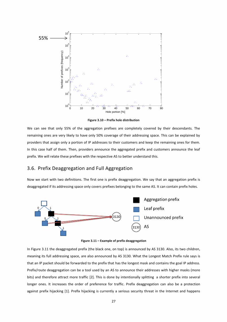
27
Figure 3.10 – Prefix hole distribution
We can see that only 55% of the aggregation prefixes are completely covered by their descendants. The
remaining ones are very likely to have only 50% coverage of their addressing space. This can be explained by
providers that assign only a portion of IP addresses to their customers and keep the remaining ones for them.
In this case half of them. Then, providers announce the aggregated prefix and customers announce the leaf
prefix. We will relate these prefixes with the respective AS to better understand this.
3.6. Prefix Deaggregation and Full Aggregation
Now we start with two definitions. The first one is prefix deaggregation. We say that an aggregation prefix is
deaggregated if its addressing space only covers prefixes belonging to the same AS. It can contain prefix holes.
Figure 3.11 – Example of prefix deaggregation
In Figure 3.11 the deaggregated prefix (the black one, on top) is announced by AS 3130. Also, its two children,
meaning its full addressing space, are also announced by AS 3130. What the Longest Match Prefix rule says is
that an IP packet should be forwarded to the prefix that has the longest mask and contains the goal IP address.
Prefix/route deaggregation can be a tool used by an AS to announce their addresses with higher masks (more
bits) and therefore attract more traffic [2]. This is done by intentionally splitting a shorter prefix into several
longer ones. It increases the order of preference for traffic. Prefix deaggregation can also be a protection
against prefix hijacking [1]. Prefix hijacking is currently a serious security threat in the Internet and happens
0 10 20 30 40 50 60 70 8010
0
101
102
103
104
105
106
Num
ber
of
pre
fixes (
frequency)
Hole portion [%]
55%

28
when an AS announces prefixes that it does not own. If the attacked AS advertises more specific routes, it is
more protected against this, since his routes have a higher preference.
The second definition is full prefix aggregation. We say that an aggregation prefix announced by AS X is fully
aggregated if its addressing space is only covered by prefixes announced by ASs other than X. It can contain
prefix holes. A similar figure is shown below, to exemplify this.
Figure 3.12 – Full prefix aggregation example
In this case, Figure 3.12 shows a fully aggregated prefix announced by AS 3130. Its two children are announced
by a different ASs, other than AS 3130. Full prefix aggregation is a good metric to understand if ASs in the
Internet are taking advantage of route aggregation to increase scalability. One can say that a fully aggregated
prefix and a deaggregated prefix are two extreme and opposite classifications of aggregation prefixes. We want
to measure the amount of prefixes in our prefix tree that fit into one of these two definitions. We also want to
know if there are prefix holes in those or not. So, we need to find an algorithm to fill Table 3.2.
With prefix holes Without prefix holes
Fully aggregated
Deaggregated
Remaining ones
Table 3.2 – Unfilled table concerning deaggregation and full prefix aggregation
To make this simpler, we can look at Figure 3.13 (below) where we can see that an aggregated prefix, 0.0.0.0/8
in the example, can only be covered by three different things: prefixes from the same AS (a), prefixes from
different ASs (b) or to not be covered at all, or in other words, to contain a prefix hole (c).
Figure 3.13 – Aggregation prefix addressing space
Unlike previous cases, we did not develop a new algorithm to solve the problem. We chose to use the same
one that we used to quantify prefix holes, with some modifications. This algorithm is only capable of counting
29
2011 2012
two different entities in an aggregation prefix (hole or no hole). This time, we want three entities, namely:
same as father-a, different than father-b, hole-c. So the easiest solution to this problem is to use the algorithm
twice. In the first call, it will count {a,b+c}. This means, it will count how many aggregation prefixes are only
filled with prefixes from the same AS and how many are only filled with prefix holes and prefixes from other
ASs. In the second call, it will count {a+c,b} in the same manner. We wo not explore this algorithm further since
it is a repetition of a previous one. The final results are presented below.
With prefix holes Without prefix holes
Fully aggregated 5.42% 11.12% 16.54%
Deaggregated 0.12% 33.22% 33.34%
Remaining ones 39.38% 10.74% 50.12%
44.92% 55.08%
Table 3.3 – Full prefix aggregation and deaggregation
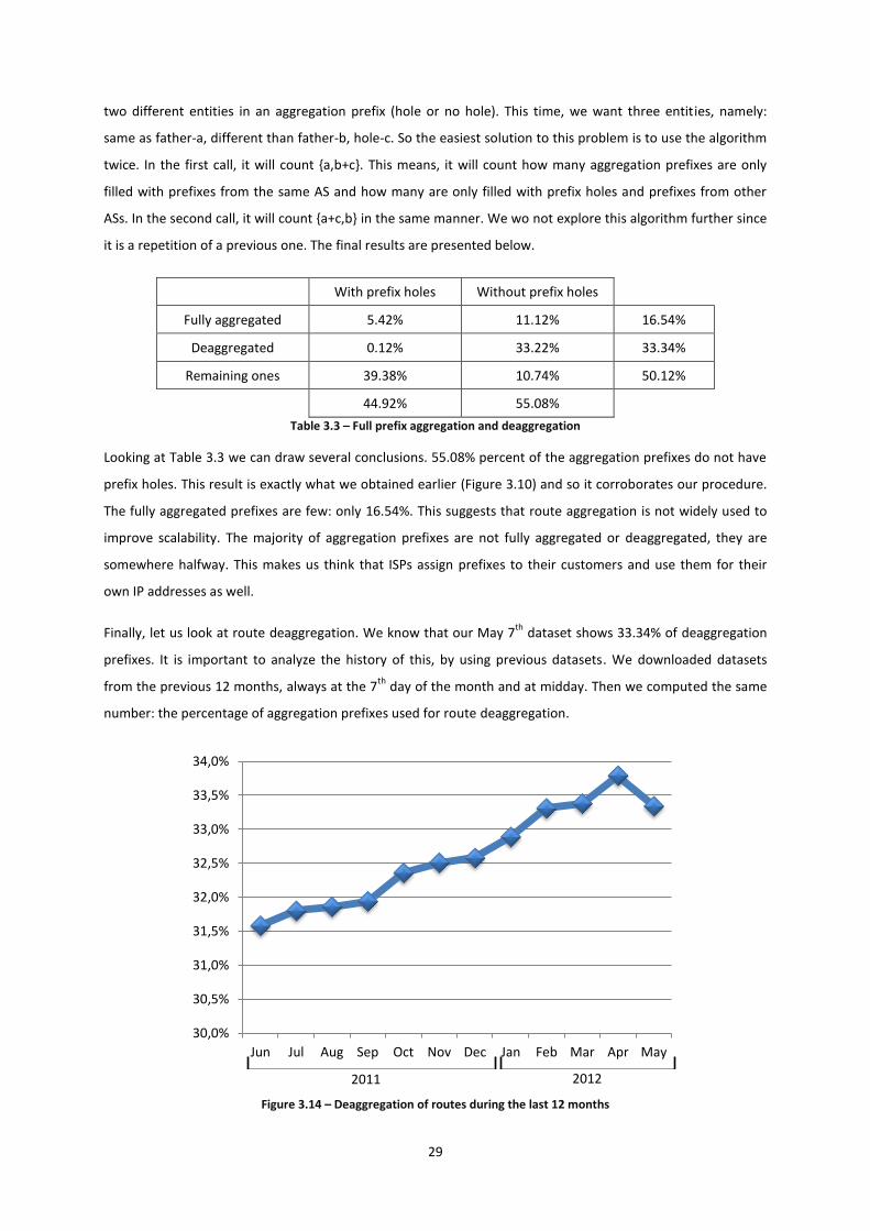
Looking at Table 3.3 we can draw several conclusions. 55.08% percent of the aggregation prefixes do not have
prefix holes. This result is exactly what we obtained earlier (Figure 3.10) and so it corroborates our procedure.
The fully aggregated prefixes are few: only 16.54%. This suggests that route aggregation is not widely used to
improve scalability. The majority of aggregation prefixes are not fully aggregated or deaggregated, they are
somewhere halfway. This makes us think that ISPs assign prefixes to their customers and use them for their
own IP addresses as well.
Finally, let us look at route deaggregation. We know that our May 7th
dataset shows 33.34% of deaggregation
prefixes. It is important to analyze the history of this, by using previous datasets. We downloaded datasets
from the previous 12 months, always at the 7th
day of the month and at midday. Then we computed the same
number: the percentage of aggregation prefixes used for route deaggregation.
Figure 3.14 – Deaggregation of routes during the last 12 months
30,0%
30,5%
31,0%
31,5%
32,0%
32,5%
33,0%
33,5%
34,0%
Jun Jul Aug Sep Oct Nov Dec Jan Feb Mar Apr May
30
It is very clear, from Figure 2.14, that deaggregation of routes is increasing at a linear pace. More and more ASs
are using this tool to perform traffic engineering, hence attracting more traffic and revenue to them. This can
compromise the scalability of the Internet.
3.7. Prefix Aggregation and Inferred Topology
So far, we have developed algorithms to help us characterize the prefix tree by itself, with a particular focus in
route aggregation. The next step is to relate it with our inferred topologies graph (we only used UCLA’s this
time). Our goal is to answer the following question: if a prefix aggregates other prefixes, what is the
relationship between the corresponding ASs? Ideally, the AS that announces the aggregated prefix should be a
provider of the other ASs. Providers assign prefixes to their direct/indirect customers within their addressing
space. The answer to this question will be very important when we study aggregation strategies, namely where
to place the aggregation node.
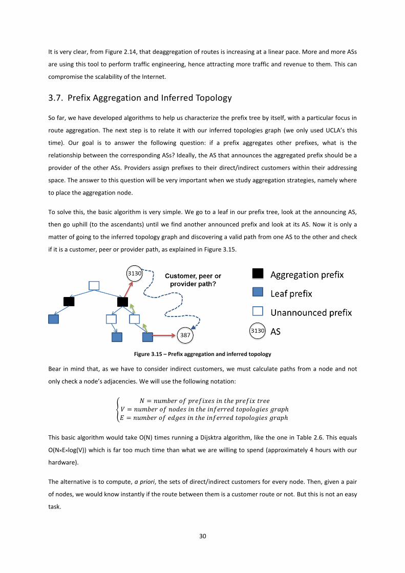
To solve this, the basic algorithm is very simple. We go to a leaf in our prefix tree, look at the announcing AS,
then go uphill (to the ascendants) until we find another announced prefix and look at its AS. Now it is only a
matter of going to the inferred topology graph and discovering a valid path from one AS to the other and check
if it is a customer, peer or provider path, as explained in Figure 3.15.
Figure 3.15 – Prefix aggregation and inferred topology
Bear in mind that, as we have to consider indirect customers, we must calculate paths from a node and not
only check a node’s adjacencies. We will use the following notation:
{
This basic algorithm would take O(N) times running a Dijsktra algorithm, like the one in Table 2.6. This equals
O(N×E×log(V)) which is far too much time than what we are willing to spend (approximately 4 hours with our
hardware).
The alternative is to compute, a priori, the sets of direct/indirect customers for every node. Then, given a pair
of nodes, we would know instantly if the route between them is a customer route or not. But this is not an easy
task.
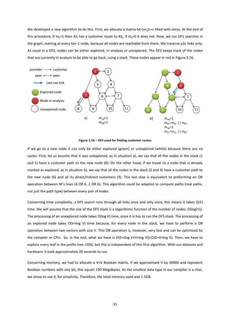
31
We developed a new algorithm to do this. First, we allocate a matrix M=[mij]V×V filled with zeros. At the end of
this procedure, if mij=1 then ASi has a customer route to ASj, if mij=0 it does not. Now, we run DFS searches in
the graph, starting at every tier-1 node, because all nodes are reachable from there. We traverse p2c links only.
As usual in a DFS, nodes can be either explored, in analysis or unexplored. The DFS keeps track of the nodes
that are currently in analysis to be able to go back, using a stack. These nodes appear in red in Figure 3.16.
Figure 3.16 – DFS used for finding customer routes
If we go to a new node it can only be either explored (green) or unexplored (white) because there are no
cycles. First, let us assume that it was unexplored, as in situation a), we say that all the nodes in the stack (1
and 5) have a customer path to the new node (8). On the other hand, if we travel to a node that is already
marked as explored, as in situation b), we say that all the nodes in the stack (2 and 4) have a customer path to
the new node (6) and all its direct/indirect customers (9). This last step is equivalent to preforming an OR
operation between M’s lines (4 OR 6, 2 OR 6). This algorithm could be adapted to compute paths (real paths,
not just the path type) between every pair of nodes.
Concerning time complexity, a DFS search runs through all links once and only once, this means it takes O(E)
time. We will assume that the size of the DFS stack is a logarithmic function of the number of nodes: O(log(V)).
The processing of an unexplored node takes O(log V) time, since it is has to run the DFS stack. The processing of
an explored node takes O(V×log V) time because, for every node in the stack, we have to perform a OR
operation between two vectors with size V. This OR operation is, however, very fast and can be optimized by
the compiler or CPU. So, in the end, what we have is O(E×(log V+V×log V))=O(E×V×log V). Then, we have to
explore every leaf in the prefix tree: O(N), but this is independent of this first algorithm. With our datasets and
hardware, it took approximately 20 seconds to run.
Concerning memory, we had to allocate a V×V Boolean matrix. If we approximate V by 40000 and represent
Boolean numbers with one bit, this equals 190 Megabytes. As the smallest data type in our compiler is a char,
we chose to use it, for simplicity. Therefore, the total memory used was 1.5GB.
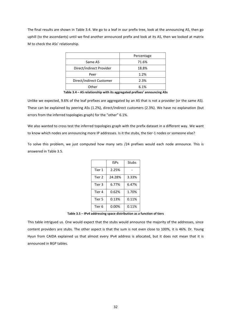
32
The final results are shown in Table 3.4. We go to a leaf in our prefix tree, look at the announcing AS, then go
uphill (to the ascendants) until we find another announced prefix and look at its AS, then we looked at matrix
M to check the ASs’ relationship.
Percentage
Same AS 71.6%
Direct/indirect Provider 18.8%
Peer 1.2%
Direct/indirect Customer 2.3%
Other 6.1%
Table 3.4 – AS relationship with its aggregated prefixes’ announcing ASs
Unlike we expected, 9.6% of the leaf prefixes are aggregated by an AS that is not a provider (or the same AS).
These can be explained by peering ASs (1.2%), direct/indirect customers (2.3%). We have no explanation (but
errors from the inferred topologies graph) for the “other” 6.1%.
We also wanted to cross test the inferred topologies graph with the prefix dataset in a different way. We want
to know which nodes are announcing more IP addresses. Is it the stubs, the tier-1 nodes or someone else?
To solve this problem, we just computed how many sets /24 prefixes would each node announce. This is
answered in Table 3.5.
ISPs Stubs
Tier 1 2.25% -
Tier 2 24.28% 3.33%
Tier 3 6.77% 6.47%
Tier 4 0.62% 1.70%
Tier 5 0.13% 0.11%
Tier 6 0.00% 0.11%
Table 3.5 – IPv4 addressing space distribution as a function of tiers
This table intrigued us. One would expect that the stubs would announce the majority of the addresses, since
content providers are stubs. The other aspect is that the sum is not even close to 100%, it is 46%. Dr. Young
Hyun from CAIDA explained us that almost every IPv4 address is allocated, but it does not mean that it is
announced in BGP tables.
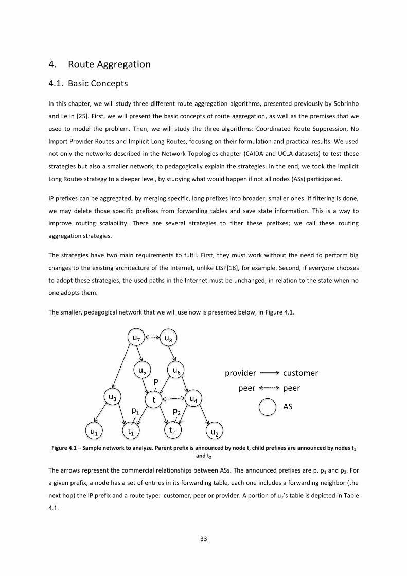
33
4. Route Aggregation
4.1. Basic Concepts
In this chapter, we will study three different route aggregation algorithms, presented previously by Sobrinho
and Le in [25]. First, we will present the basic concepts of route aggregation, as well as the premises that we
used to model the problem. Then, we will study the three algorithms: Coordinated Route Suppression, No
Import Provider Routes and Implicit Long Routes, focusing on their formulation and practical results. We used
not only the networks described in the Network Topologies chapter (CAIDA and UCLA datasets) to test these
strategies but also a smaller network, to pedagogically explain the strategies. In the end, we took the Implicit
Long Routes strategy to a deeper level, by studying what would happen if not all nodes (ASs) participated.
IP prefixes can be aggregated, by merging specific, long prefixes into broader, smaller ones. If filtering is done,
we may delete those specific prefixes from forwarding tables and save state information. This is a way to
improve routing scalability. There are several strategies to filter these prefixes; we call these routing
aggregation strategies.
The strategies have two main requirements to fulfil. First, they must work without the need to perform big
changes to the existing architecture of the Internet, unlike LISP[18], for example. Second, if everyone chooses
to adopt these strategies, the used paths in the Internet must be unchanged, in relation to the state when no
one adopts them.
The smaller, pedagogical network that we will use now is presented below, in Figure 4.1.
Figure 4.1 – Sample network to analyze. Parent prefix is announced by node t, child prefixes are announced by nodes t1
and t2
The arrows represent the commercial relationships between ASs. The announced prefixes are p, p1 and p2. For
a given prefix, a node has a set of entries in its forwarding table, each one includes a forwarding neighbor (the
next hop) the IP prefix and a route type: customer, peer or provider. A portion of u7’s table is depicted in Table
4.1.

34
Route type Next hop IP prefix Elected route
Customer u5 p1
Customer u3 p1
Peer u8 p1 - discarded, because it has
lower preference
Table 4.1 – u7’s forwarding table for prefix p1
We will use an aggregation prefix p that is announced by node t, the aggregation node. This prefix has two child
prefixes: p1 and p2 that are announced by nodes t1 and t2, respectively. These two child prefixes do not overlap,
meaning they do not share IP addressing space. So, if a node has two entries in its forwarding table with the
same route type (customer, peer or provider) to p1 and p, it will use the Longest Match Prefix rule, hence
selecting p1, for IP addresses belonging to p1. The same applies to p2. If the route type is not the same, a node
will prefer customer routes, then peer routes and only use provider routes if nothing else is available. We have
been using the same rule throughout this work. This order of preference is shown in Table 4.2.
Route type Announced prefix pi Announced prefix p
Customer 1 4
Peer 2 5
Provider 3 6
Table 4.2 – Routes' order of preference, based on commercial agreements and Longest Match Prefix rule, 1 has the highest preference
Our theory requires that the aggregation node is a direct/indirect provider of the nodes that announce its child
prefixes. This is equivalent to checking if node t’s forwarding table has customer routes to both p1 and p2. Like
we have seen in Table 3.4, this is the case for the majority of aggregation prefixes. We can say that child
prefixes announced by the aggregation nodes themselves also fit this description. According to Table 3.4, our
theory fits 90.4% (71.6%+18.8%) of the cases.
If all nodes use the aggregation strategies that we study, no paths are changed, in relation to the case when no
one uses any aggregation strategy. This will not be the case for the last topic of this chapter, concerning partial
participation.
4.2. Coordinated Route Suppression
Coordinated Route Suppression is a strategy for route aggregation that requires coordination between nodes.
It is based in the fact that if a node has the same forwarding neighbors for both parent (p) and child (p1 or p2)
prefixes, then it does not need a forwarding table entry for the child prefix. Since the neighbors are the same, a
packet addressed to a child prefix would be expedited through the same routes, according to the Longest
Match Prefix rule.
However, it is not that simple. It can occur that a node does not need the child’s forwarding table entries for
itself but there is one of its neighbors that relies on the importation of that particular child route, and therefore
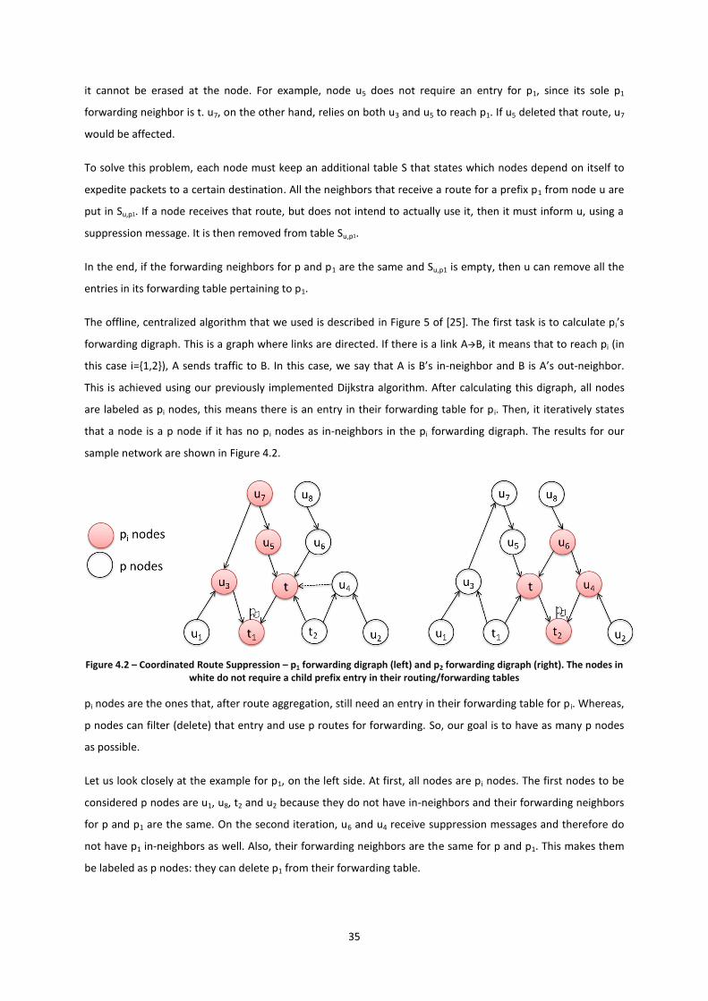
35
it cannot be erased at the node. For example, node u5 does not require an entry for p1, since its sole p1
forwarding neighbor is t. u7, on the other hand, relies on both u3 and u5 to reach p1. If u5 deleted that route, u7
would be affected.
To solve this problem, each node must keep an additional table S that states which nodes depend on itself to
expedite packets to a certain destination. All the neighbors that receive a route for a prefix p1 from node u are
put in Su,p1. If a node receives that route, but does not intend to actually use it, then it must inform u, using a
suppression message. It is then removed from table Su,p1.
In the end, if the forwarding neighbors for p and p1 are the same and Su,p1 is empty, then u can remove all the
entries in its forwarding table pertaining to p1.
The offline, centralized algorithm that we used is described in Figure 5 of [25]. The first task is to calculate pi’s
forwarding digraph. This is a graph where links are directed. If there is a link AB, it means that to reach pi (in
this case i={1,2}), A sends traffic to B. In this case, we say that A is B’s in-neighbor and B is A’s out-neighbor.
This is achieved using our previously implemented Dijkstra algorithm. After calculating this digraph, all nodes
are labeled as pi nodes, this means there is an entry in their forwarding table for p i. Then, it iteratively states
that a node is a p node if it has no pi nodes as in-neighbors in the pi forwarding digraph. The results for our
sample network are shown in Figure 4.2.
Figure 4.2 – Coordinated Route Suppression – p1 forwarding digraph (left) and p2 forwarding digraph (right). The nodes in white do not require a child prefix entry in their routing/forwarding tables
pi nodes are the ones that, after route aggregation, still need an entry in their forwarding table for p i. Whereas,
p nodes can filter (delete) that entry and use p routes for forwarding. So, our goal is to have as many p nodes
as possible.
Let us look closely at the example for p1, on the left side. At first, all nodes are pi nodes. The first nodes to be
considered p nodes are u1, u8, t2 and u2 because they do not have in-neighbors and their forwarding neighbors
for p and p1 are the same. On the second iteration, u6 and u4 receive suppression messages and therefore do
not have p1 in-neighbors as well. Also, their forwarding neighbors are the same for p and p1. This makes them
be labeled as p nodes: they can delete p1 from their forwarding table.
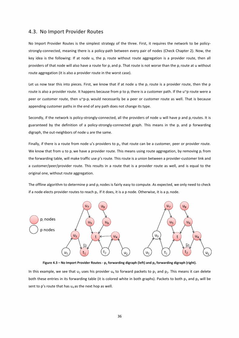
36
4.3. No Import Provider Routes
No Import Provider Routes is the simplest strategy of the three. First, it requires the network to be policy-
strongly-connected, meaning there is a policy-path between every pair of nodes (Check Chapter 2). Now, the
key idea is the following: If at node u, the pi route without route aggregation is a provider route, then all
providers of that node will also have a route for pi and p. That route is not worse than the pi route at u without
route aggregation (it is also a provider route in the worst case).
Let us now tear this into pieces. First, we know that if at node u the p i route is a provider route, then the p
route is also a provider route. It happens because from p to pi there is a customer path. If the u~p route were a
peer or customer route, then u~p-pi would necessarily be a peer or customer route as well. That is because
appending customer paths in the end of any path does not change its type.
Secondly, if the network is policy-strongly-connected, all the providers of node u will have p and pi routes. It is
guaranteed by the definition of a policy-strongly-connected graph. This means in the pi and p forwarding
digraph, the out-neighbors of node u are the same.
Finally, if there is a route from node u’s providers to pi, that route can be a customer, peer or provider route.
We know that from u to pi we have a provider route. This means using route aggregation, by removing pi from
the forwarding table, will make traffic use p’s route. This route is a union between a provider-customer link and
a customer/peer/provider route. This results in a route that is a provider route as well, and is equal to the
original one, without route aggregation.
The offline algorithm to determine p and pi nodes is fairly easy to compute. As expected, we only need to check
if a node elects provider routes to reach pi. If it does, it is a p node. Otherwise, it is a pi node.
Figure 4.3 – No Import Provider Routes - p1 forwarding digraph (left) and p2 forwarding digraph (right).
In this example, we see that u2 uses his provider u4 to forward packets to p1 and p2. This means it can delete
both these entries in its forwarding table (it is colored white in both graphs). Packets to both p1 and p2 will be
sent to p’s route that has u4 as the next hop as well.

37
4.4. Implicit Long Routes
The Implicit Long Routes is the most effective strategy. It is based on the idea that pi routes are implicitly
contained in p routes (there is a customer path from p to pi). So, when a node receives a p route, it can infer
that a pi route is also received. If a node receives a pi route from every neighbor from which it also receives a p
route, before any filtering is done, then pi routes are redundant and can be deleted from the forwarding table.
We will call these nodes R type nodes. However, if a node receives a pi route from a neighbor that did not send
a p route, the node must keep pi in its forwarding table. Also, it must take into account that p routes will stand
for themselves and for pi routes. We will call these nodes F type nodes.
The offline algorithm to determine p and pi nodes is described in Figure 6 of [25]. Basically, the objective is to
determine which links carry p routes. These links are the union of:
- Links contained in the p forwarding digraph.
- Links entering a node that has a customer route to p (a node exports his customer routes to every neighbor).
- Provider links entering a node that has a peer/provider route to p (a node exports his peer/provider routes to
every customer).
The result is pictured in Figure 4.4.
Figure 4.4 – Implicit Long Routes - p1 forwarding digraph (left) and p2 forwarding digraph (right).
We can guess that this strategy is the most effective one, since only 4 pi nodes are required for each prefix. All
the nodes in white receive p and pi routes from exactly the same neighbors. Let us look closely at u5 in the p1
forwarding digraph on the left. It receives p and p1 routes from both its neighbors u7 and t, and therefore
decides to delete p1 from its forwarding table. Now, u7 will only receive p1 from u3 and p from u5. To keep
routes unchanged, it must add an implicit entry in its forwarding table saying p1 route is also exported along
with p route from u5. Then u7 will have again 2 forwarding neighbors to reach p1.
4.5. Experimental Results
In order to cross compare the 3 strategies and use a real AS level topology, we conducted a series of tests using
both CAIDA [3] and UCLA [26] inferred graphs. As we thoroughly explained in the Network Topologies chapter,
we removed cycles and policy disconnected nodes. This gives us the guarantee that our graphs are policy-
connected and do not have forwarding loops.
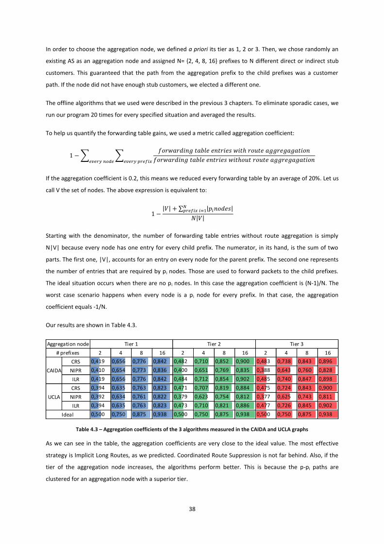
38
In order to choose the aggregation node, we defined a priori its tier as 1, 2 or 3. Then, we chose randomly an
existing AS as an aggregation node and assigned N= {2, 4, 8, 16} prefixes to N different direct or indirect stub
customers. This guaranteed that the path from the aggregation prefix to the child prefixes was a customer
path. If the node did not have enough stub customers, we elected a different one.
The offline algorithms that we used were described in the previous 3 chapters. To eliminate sporadic cases, we
run our program 20 times for every specified situation and averaged the results.
To help us quantify the forwarding table gains, we used a metric called aggregation coefficient:
∑ ∑
If the aggregation coefficient is 0.2, this means we reduced every forwarding table by an average of 20%. Let us
call V the set of nodes. The above expression is equivalent to:
| | ∑ | |
| |
Starting with the denominator, the number of forwarding table entries without route aggregation is simply
N|V| because every node has one entry for every child prefix. The numerator, in its hand, is the sum of two
parts. The first one, |V|, accounts for an entry on every node for the parent prefix. The second one represents
the number of entries that are required by pi nodes. Those are used to forward packets to the child prefixes.
The ideal situation occurs when there are no pi nodes. In this case the aggregation coefficient is (N-1)/N. The
worst case scenario happens when every node is a pi node for every prefix. In that case, the aggregation
coefficient equals -1/N.
Our results are shown in Table 4.3.
Table 4.3 – Aggregation coefficients of the 3 algorithms measured in the CAIDA and UCLA graphs
As we can see in the table, the aggregation coefficients are very close to the ideal value. The most effective
strategy is Implicit Long Routes, as we predicted. Coordinated Route Suppression is not far behind. Also, if the
tier of the aggregation node increases, the algorithms perform better. This is because the p-pi paths are
clustered for an aggregation node with a superior tier.
2 4 8 16 2 4 8 16 2 4 8 16
CRS 0,419 0,656 0,776 0,842 0,482 0,710 0,852 0,900 0,483 0,738 0,843 0,896
NIPR 0,410 0,654 0,773 0,836 0,400 0,651 0,769 0,835 0,388 0,643 0,760 0,828
ILR 0,419 0,656 0,776 0,842 0,484 0,712 0,854 0,902 0,485 0,740 0,847 0,898
CRS 0,394 0,635 0,763 0,823 0,471 0,707 0,819 0,884 0,475 0,724 0,843 0,900
NIPR 0,392 0,634 0,761 0,822 0,379 0,623 0,754 0,812 0,377 0,625 0,743 0,811
ILR 0,394 0,635 0,763 0,823 0,473 0,710 0,821 0,886 0,477 0,726 0,845 0,902
0,500 0,750 0,875 0,938 0,500 0,750 0,875 0,938 0,500 0,750 0,875 0,938
Tier 1 Tier 2 Tier 3
# prefixes
CAIDA
UCLA
Ideal
Aggregation node
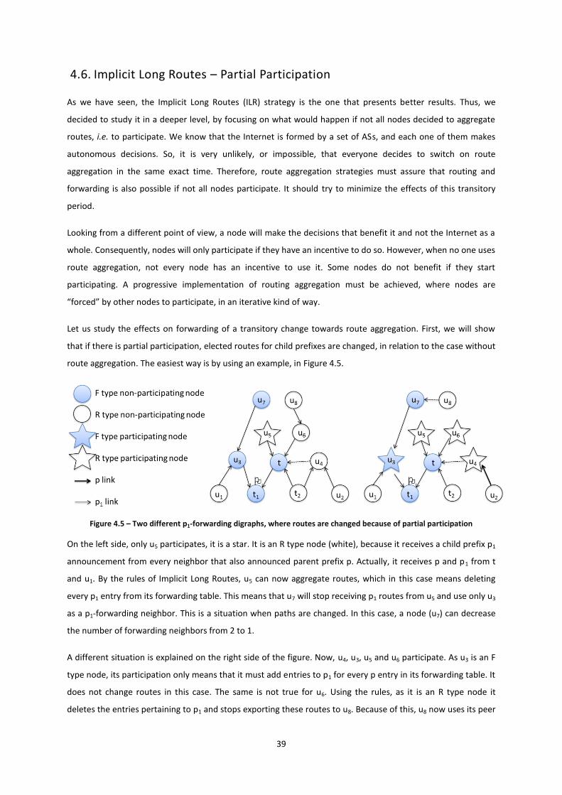
39
4.6. Implicit Long Routes – Partial Participation
As we have seen, the Implicit Long Routes (ILR) strategy is the one that presents better results. Thus, we
decided to study it in a deeper level, by focusing on what would happen if not all nodes decided to aggregate
routes, i.e. to participate. We know that the Internet is formed by a set of ASs, and each one of them makes
autonomous decisions. So, it is very unlikely, or impossible, that everyone decides to switch on route
aggregation in the same exact time. Therefore, route aggregation strategies must assure that routing and
forwarding is also possible if not all nodes participate. It should try to minimize the effects of this transitory
period.
Looking from a different point of view, a node will make the decisions that benefit it and not the Internet as a
whole. Consequently, nodes will only participate if they have an incentive to do so. However, when no one uses
route aggregation, not every node has an incentive to use it. Some nodes do not benefit if they start
participating. A progressive implementation of routing aggregation must be achieved, where nodes are
“forced” by other nodes to participate, in an iterative kind of way.
Let us study the effects on forwarding of a transitory change towards route aggregation. First, we will show
that if there is partial participation, elected routes for child prefixes are changed, in relation to the case without
route aggregation. The easiest way is by using an example, in Figure 4.5.
Figure 4.5 – Two different p1-forwarding digraphs, where routes are changed because of partial participation
On the left side, only u5 participates, it is a star. It is an R type node (white), because it receives a child prefix p1
announcement from every neighbor that also announced parent prefix p. Actually, it receives p and p1 from t
and u1. By the rules of Implicit Long Routes, u5 can now aggregate routes, which in this case means deleting
every p1 entry from its forwarding table. This means that u7 will stop receiving p1 routes from u5 and use only u3
as a p1-forwarding neighbor. This is a situation when paths are changed. In this case, a node (u7) can decrease
the number of forwarding neighbors from 2 to 1.
A different situation is explained on the right side of the figure. Now, u4, u3, u5 and u6 participate. As u3 is an F
type node, its participation only means that it must add entries to p1 for every p entry in its forwarding table. It
does not change routes in this case. The same is not true for u6. Using the rules, as it is an R type node it
deletes the entries pertaining to p1 and stops exporting these routes to u8. Because of this, u8 now uses its peer

40
u7 (and not its customer u6) to reach p1. This is a second scenario where routes were changed. Now, a node (u8)
changed its route type (from customer to peer route).
So, we know that nodes can see their routes changed by the number of forwarding neighbors and the route
type. We will use these two metrics to quantify path distortion.
Looking at incentives, nodes u5 and u6 have motivation to participate, because their forwarding neighbors will
not change and they can save space in their forwarding table. Also, they will stop receiving packets from u7 and
u8, which are their providers and therefore do not pay for traffic. On the other hand, u3 has no reason to
participate, despite not changing its routes.
The thing left unnoticed is the participation of u4. It has a different consequence; u4 is R type, so it stops
exporting p1-routes to its customer u2. Now, u2 has no neighbors to forward packets to p1. Using the Longest
Match Prefix rule, u2 now has to forward packets using p routes. It “aggregates” routes without even
participating. If a node elects a p route, ILR guarantees that the route is equal to the original p1 route.
To test partial participation, the very first thing to do is to compute the full participation p1-forwarding digraph.
Then, we need to use the offline ILR algorithm previously presented; this will tell us which are the R and F type
nodes. They were p and pi nodes before, respectively. Now, what we need to do is the following: if a type R
node chooses to participate, all the links entering it are removed from the original graph. If the node is type F,
nothing happens. Notice that in Figure 4.5, when a white circle became a white star, all the pi links entering it
were removed. After this, all we need to do is compute the p1-forwarding digraph, using the same Dysktra
algorithm but with an input graph with fewer links. In the end, we look at Table 4.4 to quantify the results for
every node u.
In the p1 full participation digraph:
- Node u elects forwarding neighbors
using route type
In the p1 partial participation digraph:
- Node u elects forwarding neighbors
using route type
Possibilities Consequence
Nothing happens
+1 change number of neighbors
+1 change of route type
Nothing happens (p route is elected)
Table 4.4 – Quantifying path distortion as a consequence of partial participation of route aggregation
Our last metric is the aggregation coefficient. For this, we just need to know which nodes are pi nodes. A simple
solution is presented in Table 4.5.
R type node F type node
Participating node p node pi node
Non-participating node p node if n’=0
pi node if n’>0 pi node
Table 4.5 – Labeling nodes as p or pi nodes, n’ is defined in Table 4.4

41
It is easy to understand that if a node is F type, it will always be a pi node, since it cannot aggregate routes. The
tricky part is the non-participating R type nodes, which was already exemplified. These nodes can be in a
situation where they do not receive pi routes from anyone. Even though they do not participate, they do not
have a pi route in their forwarding table.
Our first attempt to choose participating nodes was very simple. We used a scenario where only stub nodes
(nodes with no customers) would participate. The results are below.
We notice that aggregation coefficients are very high. This is because stubs are 80% of the total number of
nodes and they are all R type nodes, if you ignore occasional peer links. This is because all their providers
announce pi and p routes, since the graph is policy-connected. Also, as stubs do not export routes to their
providers, the original routes are not distorted.
Our second (and final) attempt to choose participating nodes is more complex. We wanted to compute the
aggregation coefficient, the number of nodes that change route type and number of forwarding neighbors as 3
functions of the percentage of participating nodes.
The mechanics of this are the following: we start with 0% participation and compute the three metrics. Then,
we iteratively add an additional, randomly chosen, 1% as participating nodes and do the same. The process
ends in 100%, obviously.
Presenting all the results would be a fastidious task, since we have 24 different plots. Thus, we only present
three interesting ones in Figure 4.6.
Aggregation node Tier 1 Tier 2 Tier 3
# prefixes (N) 2 4 8 16 2 4 8 16 2 4 8 16
CA
IDA
Aggregation Coefficient 0.295 0.540 0.661 0.722 0.328 0.578 0.698 0.764 0.339 0.586 0.712 0.786
#change route type 0
#change #neighbors
UC
LA
Aggregation Coefficient 0.274 0.524 0.651 0.713 0.318 0.569 0.693 0.757 0.333 0.579 0.706 0.834
# change route type 0
# change #neighbors
Table 4.6 – Aggregation coefficient and path distortion for only stub nodes participating in ILR route aggregation

42
Figure 4.6 – ILR Partial Participation metrics using UCLA’s inferred topology graph. Top: Tier 2 aggregation node, 8 child prefixes. Center: Tier 3 aggregation node, 2 child prefixes. Bottom: Tier 3 aggregation node, 8 child prefixes
0 10 20 30 40 50 60 70 80 90
-0.1
0
0.1
0.2
0.3
0.4
0.5
0.6
0.7
0.8
0.9
Participating ASs (%)
Aggre
gation C
oeff
icie
nt
0
5
10
15
20
AS
s t
hat
change r
oute
type (
%)
0
5
10
15
20A
Ss t
hat
change t
he n
um
ber
of
forw
ard
ing n
eig
hbors
(%
)
0 10 20 30 40 50 60 70 80 90-0.5
0
0.5
1
Participating ASs (%)
Aggre
gation C
oeff
icie
nt
0
5
10
15
20
AS
s t
hat
change r
oute
type (
%)
0
5
10
15
20
AS
s t
hat
change t
he n
um
ber
of
forw
ard
ing n
eig
hbors
(%
)
0 10 20 30 40 50 60 70 80 90
-0.1
0
0.1
0.2
0.3
0.4
0.5
0.6
0.7
0.8
0.9
Participating ASs (%)
Aggre
gation C
oeff
icie
nt
0
5
10
15
20
AS
s t
hat
change r
oute
type (
%)
0
5
10
15
20
AS
s t
hat
change t
he n
um
ber
of
forw
ard
ing n
eig
hbors
(%
)

43
Now it is easier to understand how ILR behaves if not everyone participates. Just to double check our theory
and programming, we can see that:
- The blue and pink graphs, that measure distortion in paths, have zeros in 0 and 100%. This is congruent with
our theory, which states that paths are not changed if everyone participates.
- The aggregation coefficient is a monotonically increasing function. This happens because the participation of a
node cannot increase the average forwarding table size.
Well, the first things that we noticed in the plots were the sudden steps. After debugging the actual source
code, we understood that these were caused by the new participation of either tier-1 nodes or nodes that
were forwarding traffic near the aggregation node.
We can also see that the maximum distortion is reached at approximately 35% participating ASs. It is also
common to the omitted graphs.
Because of the phenomena that we have described in Table 4.5, some nodes can “aggregate” routes without
participating (they do not receive pi routes). If this did not happen, the aggregation coefficient plot would be a
straight line. Whereas, the maximum aggregation coefficient is almost reached at 80% participating nodes.

44
45
5. Conclusion
To finish, let us summarize the main results of each chapter.
In Chapter 2, we analyzed two inferred topologies graphs: CAIDA and UCLA. UCLA has more data sources and
therefore captures more links. It also updates daily, unlike CAIDA, whose dataset was 1.5 years old. They also
use different inference algorithms: CAIDA tries to find a balance between maximizing the number of valid paths
and adjusting commercial relationships to node degrees[6]. UCLA, on the other hand, establishes a tier-1
network and then infer links from valid paths using tier-1 BGP tables[17]. To use these datasets later, as input
data, we had to remove cycles and policy-disconnected nodes. In the end, we noticed that there is a 53%
probability that a random path in the Internet contains tier-1 nodes. Also, if we remove tier-1 nodes, a node
cannot communicate with 15.6% of the Internet.
In Chapter 3, we looked at the Internet IPv4 prefix announcements (captured by RouteViews), focusing on
prefix aggregation. We constructed a binary tree to represent this data. We noticed that we can have 7
aggregation levels. Also, only 55% of the aggregation prefixes completely cover their descendants. Prefix
aggregation is not being used mainly to increase scalability, since only 16.54% are fully aggregated and 33% of
aggregation prefixes are deaggregated. Then, we crossed this data with inferred topologies. If we look at a
random leaf prefix, there is a 71.6% probability that its aggregation prefix, if it has one, is announced by the
same AS and 18.8% by a direct/indirect provider. Ideally these two numbers should sum up to 100%. On a
different subject, we noticed that the majority of IPv4 addressing space is allocated to ISP’s and not stub ASs.
In Chapter 4, we looked at Sobrinho and Le’s work in [25] and went a bit further. We tested three different
aggregation strategies: Coordinated Route Suppression, No Import Provider Routes and Implicit Long Routes.
We used the inferred topologies, previously processed, to quantify the results in terms of savings in forwarding
tables’ sizes. These were very close to the ideal. The most effective strategy, Implicit Long Routes, was tested
further. We simulated an Internet where only tier-1 nodes participated in route aggregation and measured
savings and path distortion. Savings were inexistent and distortion was high. Then, we did the same for stub AS
participating, it was the other way around, savings were high and distortion was null. To conclude, we obtained
plots where distortion and savings were measured, in function of the percentage of participating ASs. We
noticed that changes were sudden (like steps), maximum distortion at 35% participation, and maximum savings
almost reached at 80% participation.

46

47
6. Future Work
In chapter 3, we studied prefix to AS mappings from CAIDA[4], which is combined information of RouteViews
forwarding tables[23]. Because of this combination, some information is lost, namely, which peer ASs receive
each prefix. The total number of peer ASs is 45. We did a quick look-up on RouteViews data and we concluded
that not all 45 peers can capture every prefix. This is a proof that filtering is done. An in-depth study about this
would be a relevant subject to explore in future work.
Concerning aggregation strategies, we have proved that Implicit Long Routes is most promising one. The most
relevant subject that we did not analyze is incentives. We would study the adoption of ILR from a different
point of view, using Game Theory. It is very clear that if everyone participates in Route Aggregation, every AS
would benefit, but that is not true for the case when only a portion of ASs participate, as we have seen. An AS
can have several benefits that make it participate: it can save space in its forwarding table, or it increase its
number of forwarding neighbors, or change its route type (but this time for a better one).

48
7. Bibliography
[1] H. Ballani, P. Francis, and X. Zhang. “A Study of Prefix Hijacking and Interception in the Internet”.
Proceedings of ACM SIGCOMM, pp. 265–276, 2007.
[2] L. Cittadini, W. Muhlbauer, S. Uhlig, R. Bush, P. Francois, O. Maennel. “Evolution of Internet Address Space
Deaggregation: Myths and Reality”. IEEE Journal on Selected Areas in Communications, vol. 28, no. 8, pp.
1238–1249, October 2010.
[3] The CAIDA AS Relationships Dataset, January 16, 2011.
http://www.caida.org/data/active/as-relationships/
[4] CAIDA, Routeviews Prefix to AS mappings Dataset, May 7, 2012.
http://www.caida.org/data/routing/routeviews-prefix2as.xml
[5] X. Dimitropoulos, M. Angeles Serrano, and D. Krioukov. “On cycles in AS relationships”. ACM SIGCOMM
Computer Communication Review, vol. 38, no. 3, pp. 102–104, July 2008.
[6] X. Dimitropoulos, D. Krioukov, M. Fomendov, B. Huffaker, Y. Hyun, and kc claffy. “AS relationships:
Inference and validation”. ACM SIGCOMM Computer Communication Review vol. 37, no. 1, pp. 29–40,
January 2007.
[7] Richard P. Draves, Christopher King, Srinivasan Venkatachary, Brian D. till, “Constructing Optimal IP
Routing Tables”. Proceedings of ACM CoNEXT, pp. 88–97, March 1999.
[8] A. Elmokashfi, A. Kvalbein, C. Dovrolis, “On the Scalability of BGP: The Roles of Topology Growth and
Update Rate-limiting”. Proceedings of ACM CoNEXT, pp. 1–12, 2008.
[9] L. Gao, “On inferring autonomous system relationships in the Internet”. IEEE/ACM Transactions on
Networking, vol. 9, no. 6, pp. 733-745, December 2001.
[10] Z. Ge, D. Figueiredo, S. Jaiwal, and L. Gao. “On the Hierarchical Structure of the Logical Internet graph”.
Proceedings of SPIE ITCOM, vol. 4526, pp. 208-222, August 2001.
[11] Hamed Haddadi, Damien Fay, Steve Uhlig, Andrew Moore, Richard Mortier and Almerima Jamakovic.
“Mixing Biases: Structural Changes in the AS Topology Evolution”. Traffic Monitoring and Analysis, Lecture
Notes in Computer Science, 2010, Volume 6003/2010, pp. 32-45, April 2010.
[12] Geoff Huston. “Interconnection, peering, and settlements”. Proceedings of INET, vol.{1, 2}, pp.{2-17,2-24},
June 1999.
[13] Franck Le, Geoffrey G. Xie, Hui Zhang. “On route aggregation”. Proceedings of ACM CoNEXT, pp.23-31,
2011.

49
[14] D. Jen, M. Meisel, H. Yan, D. Massey, L. Wang, B. Zhang, L. Zhang. “Towards a New Internet Routing
Architecture: Arguments for Separating Edges from Transit Core”. Proceedings of ACM Workshop on Hot
Topics in Networks -VII, pp.1-6, October 2008.
[15] F. Kamoun, L. Kleinrock. “Hierarchical Routing for Large Networks: Performance Evaluation and
Optimization”. Computer Networks, vol. 1, pp. 155–174, January 1977.
[16] V. Khare, D. Jen, X. Zhao, Y. Liu, D. Massey, L. Wang, B. Zhang, L. Zhang. “Evolution Towards Global Routing
Scalability”. IEEE Journal on Selected Areas in Communications, vol. 28, no.8, pp. 1363 –1375, October
2010.
[17] R. Oliveira, D. Pei, W. Willinger, B. Zhang, and L. Zhang. “The (in)Completeness of the Observed Internet
AS-level Structure,” IEEE/ACM Transactions on Networking, vol. 18, pp. 109-122, February 2010.
[18] D. Meyer, “The Locator Identifier Separation Protocol (LISP).” Internet Protocol Journal, vol. 11, no. 1,
March 2008.
[19] D. Meyer, L. Zhang, K. Fall. “Report from the IAB Workshop on Routing and Addressing”. RFC 4984,
September 2007.
[20] Y. Rekhter, T. Li. “An Architecture for IP Address Allocation with CIDR”. RFC 1518, September 1993
[21] Y. Rekhter, et al. "Address Allocation for Private Internets". RFC 1918, February 1996
[22] “RIPE-RIS”. http://www.ripe.net/data-tools/stats/ris
[23] RouteViews Prefix to AS mappings Dataset (pfx2as), May 7, 2012.
http://www.caida.org/data/routing/routeviews-prefix2as.xml
[24] Robert Sedgewick. “Algorithms in C”. 3rd
Edition.
[25] João L. Sobrinho, Franck Le. “A Fresh Look at Inter-Domain Route Aggregation”. INFOCOM 2012 mini-
conference, March 2012.
[26] UCLA Internet Topology Collection, May 7, 2012.
http://irl.cs.ucla.edu/topology/
[27] “University of Oregon RouteViews project”.
http://www.routeviews.org/
[28] Wikipedia, the free encyclopedia. “Tier 1 network”.
http://en.wikipedia.org/wiki/Tier_1_network
[29] B. Zhang, R. Liu, D. Massey, and L. Zhang. “Collecting the Internet AS-level topology”. ACM SIGCOMM
Computer Communication Review, vol. 35, pp. 53–61, January 2005.

50
[30] X. Zhao, Y. Liu, L. Wang, B. Zhang. “On the Aggregatability of Router Forwarding Tables”. Proc. IEEE
INFOCOM, 2010.