Embed Size (px)
Citation preview
DOUGLAS PAPER 4431REVISED SEPTEMBER 1968
"IP DDC
FEB 61969
COMPLETE SYSTEM ANALYSIS:QUANTITATIVE SYSTEM ANALYSIS,
COMPUTER SIMULATION, AND SYSTEM OPTIMIZATION
A.F. GOODMAN
L. GAINENC.O. BEUM, JR.
Presented toLos Angeles Section
American Institute of Aeronautics and Astronautics1967 Lecture Series,
"Statistical Methods in Modern Engineering"
Los Angeles. CaliforniaMarch 7. 1967
Tiedocrnieni )'aq boen approvedpnb1,- r~r,-!•-. ~''�-"10e; its
&WAvdlable CopyBestA a•ata"'---.''"•• .':.,,MaCOONRIErLL D@UO
4 S)lIE.....
MCDONNELL DOUGLAS ASTWONAUJrCOS COMP4ANYsweirrVE awUoo
Reproduced by theCLEARINGHOUSE
for Federal Scie,,tific & Technical
THIS DOCUMENT CONTAINED Information Springfield Va. 22151
BLANK PAGES THAT HAVE
BEEN DELETED
W'3' 313, IOn
101 1#3FF SECTION [Q
! ?: ......... ..*......°......
S.. ..... °... ............... o. ....
USTR1111I01H!AVAILA3ILI1y CODES
lIST. AVAIL. didK SPECIAK
ALSO INVITED FOR PRESENTATION TO:
LOS ANGELES CHAPTER OF THE ASSOCIATION FOR COMPUTING MACHINERY PANELDISCUSSION, "SIMULATION: IT'S PROBLEMS AND POTENTIAL." ON 5 APRIL 1967.
LOS ANGELES SECTION OF THE INSTITUTE OF ELECTRICAL AND ELECTRONICENGINEERS PROFESSIONAL GROUP. SYSTEM SCIENCE AND CYBERNETICS. ON20 APRIL 1967, 18 MAY 1967, AND 15 JUNE 1967.
SAN DIEGO SECTION OF THE AMERICAN INSTITUTE OF AERONAUTICS AND ASTRONAUTICS1967 LECTURE SERIES. "STATISTICAL METHODS IN MODERN ENGINEERING." ON 3 MAY 1967.
UNIVERSITY OF CALIFORNIA ENGINEERING AND PHYSICAL SCIENCES EXTENSION%,OURSE NO. 898, "MODERN SYSTEMS THEORY AND ITS APPLICATION TO LARGESCALE SYSTEMS," ON 10 JULY 1967.
STATISTICAL PROGRAM EVALUATION COMMITTEE, ON 9 JANUARY 1968.
U
COMPLETE SYSTEM ANALYSIS: QUANTITATIVE SYSTEM ANALYSIS,COMPUTER SIMULATION, AND SYSTEM OPTIMIZATION*
by
A. F. Goodman
Senior Technical Staff to Vice PresidentInformation Systems Subdivision
McDonnell Douglas Astronautics Company - Western Division
L. GainenManager, Modeling and Simulation
Information Systems SubdivisionMcDonnell Douglas Astronautics Company - Western Division
C. 0. Beum, Jr.Space Research Scientist, Development System Engineering
System Engineering ManagementNorth American Rockwell Corporation - Space Division
ABSTRACT
Many systems anr7 processes in use today are quite complex, and experimen-
tation regarding them is both difficult and expensive. For such systems or
processes, mathematical solution for outputs in terms of inputs is usually
not feasible, and computer simulation is often an effective and efficient com-
plement to experimentation.
Complete system analysis is a general approach to the coorditiation of
experimentation and computer simulation in the analysis and optimihation of
a system or process. In addition, it is somewhat novel in its approach.
Three basic stages of complete system analysis are quantitative system
analysis, computer simulation, and system optimization.
'This paper is the overview of a one-semester course, given by the authorsfor the Operations Research and Statistics Department of California StateCollege at Long Beach. Complete systen-. analysis and quantitativ'e! systemanalysis are discussed by Dr. Goodman; computer simulation, byMr. Gainen; and system optimization, by Mr. Beum.
Quantitative system analysis transforms qualitative elements of the systeminto numerical form, and constructs a system model for relationships amongcomponent parts of the system. It is a comprehensive and definitive approach
to model construction.
It is followed by computer simulation transforming the model, which is amathematical representation of the system, into a simulation computer pro-
gram, which is a computer representation of the system. Experimentation
with the system may then be complemented by computer simulation of the
system.
Finally, system optimization is accomplished by the optimization of a
meaningful measure of system effectiveness. This optimization may be
accomplished by mathematical techniques for simple systems. For complex
systems, however, optimization requires iterative repetition of system
experimentation and simulation, analysis, and improvement.
During the design of a complex system, the system does not yet exist andexperimentation regarding it is impossible. The approach of complete
system analysis then may be modified to yield complete system design, a
meaningful framework for the utilization of computer simulation in the design
of a complex system.
ii
INTRODUCTION
Many systems and processes in use today are quite complex. and experimen-
tation regarding them is both difficult and expensive. For such systems or
processes, mathematic.al solution for outputs in terms of inputs is usually
not feasible, and computer simulation is often an effective and efficient com-
plement to experimentation.
When the model of the system or process is translated into a simulation
computer program, the system or process and the effects of various factors
upon it may be simulated. The accuracy and precision of the computer
simulation increase as the accuracy and precision of the model increase.
"rhere are four periods or phases in the life cycle of a system or process--
research, development. operation. and replacement. In like manner, there
are four periods or phases in the evolution of one's knowledge concerning an
existing system or process--description, modeling, prediction, and control
and optimization. Computer simulation yields appropriate results in all four
periods of the life cycle, and in the latter three periods of the evolution of
knowledge.
Complete system analysis is a general approach to the coordination of exper-
irnentation and computer simulation in analysis and optimization of a system
or process. In addition. it is somewhat novel in its approach. Three basic
stages of complete system analysis are quantitative system analysis, com-
puter simulation, and system optimization.
Quantitative system analysis transforms qualitative elements of the system
into numerical form. and constructs a system model for relationships among
component parts of the system. It is a comprehensive and definitive approach
to model construction.
--wI III I
A detailed structure is developed for the system by arranging system elements
into an informative order. A numerical description then is defined for the
detailed structure by associating a number with each ordered qualitative
element. Component parts of the system are arranged into an informative
and unifying order to form a general structure. To simplify the specificati.
and estimation of a system model, related component parts are combined
whenever feasible. A system model is constructed by specifying relationships
among component parts in the general structure. The relationships are
expressed as mathematical equations containing unspecified constants.
Computer simulation transforms the model, which is a mathematical rep-
resentation of the system, into a simulation computer program, which is a
computer representation of the system. Experimentation with the system
may then be complemented by computer simulation of the system.
Finally, system optimization is accomplished by the optimization ,.f a mean-
ingful measure of system effectiveness. This optimization may be accom-
plished by mathematical tech~liques for simple, systems. For complex
systems, however, optimization requires iterative repetition of system
experimentation and simulation, analysis, and improvement.
During the design of a complex system, the system does not yet exist and
experimentation regarding it is impossible. The approach of complete
system analysis then may be modified to yield complete system design, a
meaningful framework for the utilization ol computer simulation in the design
of a complex system.
2
COMPLETE SYSTEM ANALYSIS
INTRODUCTION
Complete system analysis provides a logical and informative mechanism for
augmenting experimentation with computer simulation. It supplies the frame-
work of a program for constructing and estimating a model, developing a
simulation computer program, validating the model and simulation computer
program, performing experimental and simulation trials, and analyzing
experimental and simulation data. It also includes iterative improvement of
the system, and design of additional experimental and simulation trials.
An outline of complete system analysis is followed by an overview of it,
and a brief discussion of it and it's modification for systein design.
OUTLINE
Complete system analysis, as illustrated by Figure 1, is composed of eleven
basic stages:
1. Quantitative system analysis to transform qualitative elements of thesystem into numerical form and to construct a model, with unspeci-fied constants, )r relationships among component parts of the system.
Z. Experimental trial(s) to yield experimental data.
3. -Model estimation to produce estimates of unspecified constants inthe model from experimental data and available auxiliary data, andto perform a preliminary evaluation of the model's adequacy.
4. Simulation programming to construct a simulation computer programfrom the model.
5. Simulation trial(s) to yield simulation data.
6. Model and simulation data comparison to provide a validation(positive check) for the simulation computer program.
7. Experimental and simulation data comparison to provide a validationfor the combination of model and simulation computer program.
3
II• | I ESTIMATI[ON AND SIMULATION
MINTAL SYTM AND SKIULATHIM SIMUILATION SSETIA( RI111 ATA COMPANISON SYTI TRIAL(S IMLAIO
"44•,e4• DATA ANALYSIS DATA ANALYSIS ,l• b'
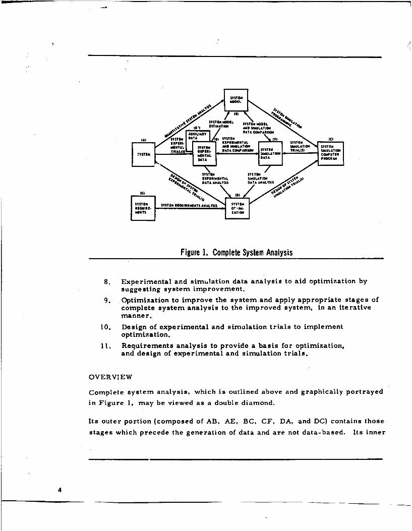
Figure 1. Complete System Analysis
8. Experimental and simulation data analysis to aid optimization bysuggesting system improvement.
9. Optimization to improve the system and apply appropriate stages ofcomplete system analysis to the improved system, in an iterativemanner.
10. Design of experimental and simulation trials to implementoptimization.
11. Requirements analysis to provide a basis for optimization,and design of experimental and simulation trials.
OVERVIEW
Complete system analysis, which is outlined above and graphically portrayed
in Figure 1, may be viewed as a double diamond.
Its outer portion (composed of AB, AE, BC, CF, DA, and DC) contains those
stages which precede the generation of data and are not data-based. Its inner
4
portion (composed of EB, BF, EF, ED, and FD) contains those stages which
follow the generation of data and are data-based.
The model and simulation computer program are developed and validated
by means of stages which comprise the upper portion of the double diamond
%AB, AE, E!., BC, CF, BF, and EF). Analysis of data, and design ofexperimental and simulation trials to optimize the system, are performed by
those stages which comprise the lower portion of the double diamond (ED,
FD, DA, and DC).
Development of the model and design, performance and analysis of experi-
mental trials are accomplished by those stages in the left-hand portion (AI'e
AE, EB, ED, and DA). Finally, the right-hand portion (BC, CF, BF, EF,
FD, and DC) contains those stages concerned with developing and validating
the simulation computer program, and with designing, performing and ana-
lyzing simulation trials.
The inherent symmetry and simplicity of the double diamond make it a very
meaningful and suggestive way in which to view complete system analysis.
DISCUSSION
Let the system be composed of components, the components contain compo-
nent parts, and the cormponent parts have elements. (Deeper levels of
system composition could be considered, if necessary.)
The transformation of qualitative system elements into numerical form is
accomplished in two steps:
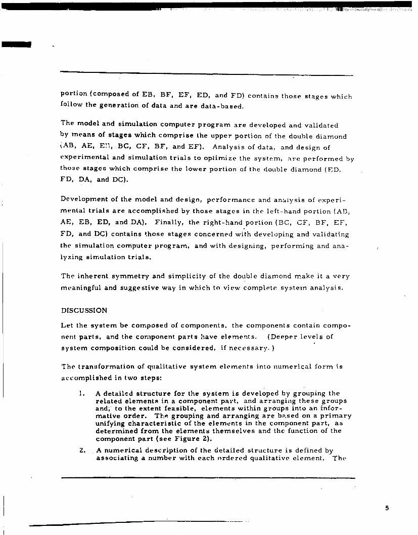
1. A detailcd structure for the system is developed by grouping therelated elements in a component part, and arranging these groupsand, to the extent feasible, elements within groups into an infor-mative order. The grouping and arranging are based on a primaryunifying characteristic of the elements in the component part, asdetermined from the elements themselves and the function of thecomponent part (see Figure 2).
Z. A numerical description of the detailed structure is defined byassociating a number with each ordered qualitative element. The
5
S......... C0OYPON EN• PAR;T L,_GROUP _F i__ _L A___[_ GRLE%,IENT :
SYSTEM ~~COM.PtNENT PA''ii]11111SYSTEM I
~~ I~E~]E] ELEMENT [[ D ISrCl, E 2 1 E] E 4] D_ O [9 E] 0• F] N-
MCI 3 nC 4rE C15 - F1 51 F1 ý
C IS AN ABBREV':ATION FOR COMPONENI PART.
Fig~ure 2. Arrangement of Elements to Form a Detailed Structure
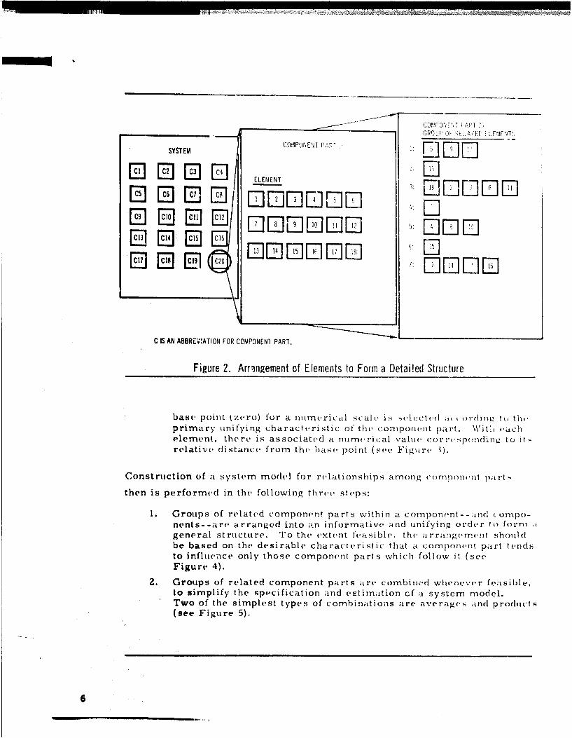
base point tzero) for a numerical sLcale- is seltected at,, ordingz to, tht,primary unifying characteristic of thv coniponent part. Witit (-achelement, there is associated a nuLmerical vpalue colrc-.spwid-.1,1 to jtý-relative distance frorn the base. point (sev F~igu~re. ).
Construction of at system model for relationships among comnpone~nt partst
then is performed in the following three steps:
1. Groups of related component parts within a componen~t--and compo-nents-°are arranged into a•n informative and unifying order !,o form• tgeneral structure. ro the extent feasible. the arrangaement shouldbe based on the desirable characteristic that a component part tendsto inflUen.ce only those component parts which follow it (see,Figure 4).
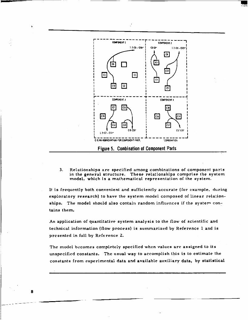
Z. Groups of related component parts are combine:d whenever feasible,to simplify the specification and estimnation cf ai system model.Two of the simplest types of combinations are average.s itnd products(see Figure 5).
6W~i
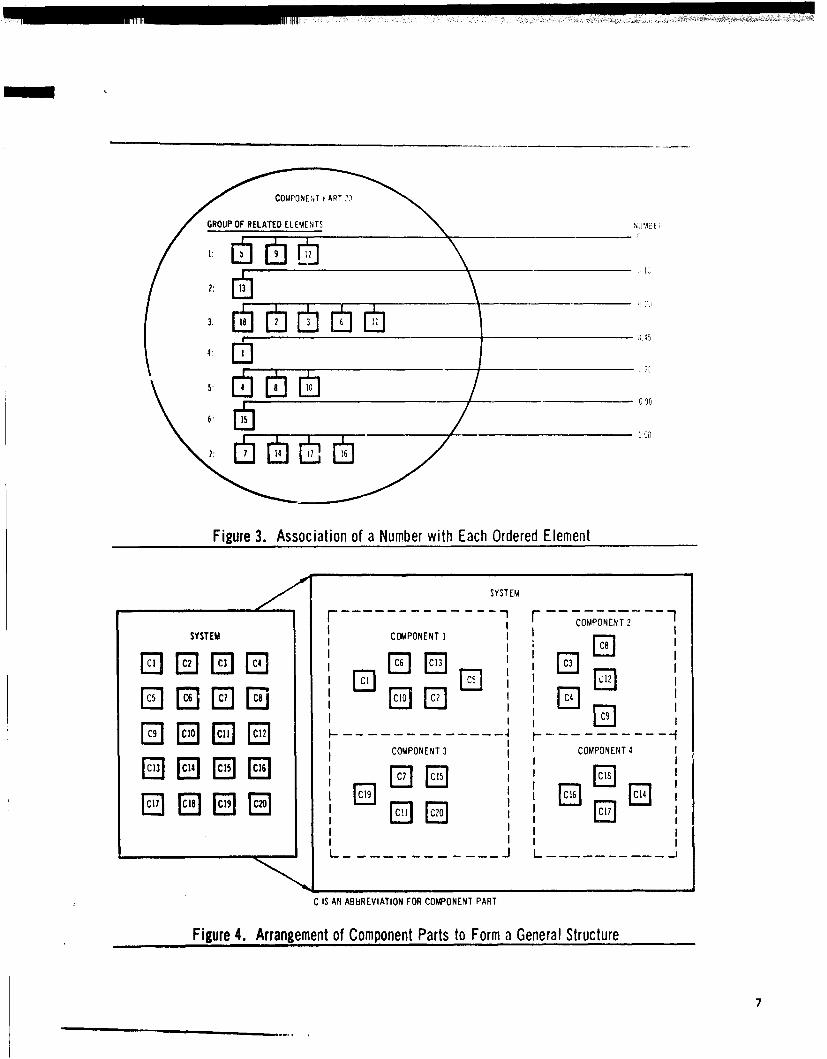
Figure 3. Association of a Number with Each Ordered Element
S~SYSTEM
O COMPONENT A
SYSTEM ICOMPONENT I I
GRU OF REL rD EL EMNT
Fiue3 sscain of MPONumeihEach Oree ElemPOent
-.................
COMPOENT3COMPONENT2
TIS AN ABREVIATION FOR COMP ONENT PART
Figure 4. Arrangement of Component Parts to Form a General Structure
E] ... 31C3
COWONENT I r*- COMPONENT 7
I 2rC6. ClOr C3C4" I 2 -C .CI2M"
C El
f C4
CI I
COMPONENT 4 COMPONfENT 4
I? C? CII ci
el5 C20 " eL7 C
1 M(7 - CIIV
C IS AN ABBREVIATION FOR COMPONENT PART. COMe•INATION
Figure 5. Combination of Component Parts
3. Relationships are specified among combinations of component partsin the general structure. These relationships comprise the systemmodel, which is a mathematical representation of the system.
It is frequently both convenient and sufficiently accurate (for example, during
exploratory research) to have the system model composed of linear rela'zion-
ships. The model should also contain random influences if the system con..
tains them.
An application of quantitative system analysis to the flow of scientific and
technical information (flow process) is summarized by Reference I and is
presented in full by Reference 2.
The model becomes completely specified when values are assigned to its
unspecified constants. The usual way to accomplish this is to estimate the
constants from experimental data and available auxiliary data, by statistical
8
estimation techniques (for example, regression analysis), A system model
which admits good estimators of its unspecified constants is preferable to a
more exact one which admits only poor estimators.
A simulation computer program transforms the model's mathematical rep-
resentation of the system into a computer representation of the system.
Input data is required for the simulation computer program to produce a
simulation trial.
Although frequently overlooked or ignored, validation should be provided for
the model and simulation computer program. When the simulation computer
program has been validated to assure that it adequately represents the sys-
tem model, the combination of model and simulation computer program
should be validated to assure that the combination adequately represents the
system. The required comparisons, of the model and simulation data followed
by that of experimental and similation data, are performed by statistical
testing techniques (for example, analysis of variance). When the system and
model contain random influences, the same inputs may yield different sets of
experimental and simulation data, and validation comparisons should take
this randomness of the data into account. Experimental and simulation data
analysis aids optimization by suggesting improvement of the system. The
analysis is accomplished by both statistical estimation and testing techniques.
Since few systems cannot be improved, one of the most important stages is
optimization through iterative improvement of the system and repetition of the
appropriate stages of complete system analysis. The design of experimental
and simulation trials is, of course, achieved by the techniques of statistical
design of experiments.
Chapter 2 of Reference 3 describes the planning of computer simulation
trials in a manner similar to that of complete system analysis.
During the design of a complex system, thzs system does not yet exist and
"experimentation regarding it is impossible. The system is replaced by
9
SY ST 9. 4MOEM'O.YSTE i OD E L
-q•, SPE CIFICATIONS SIMUDAD LATIONDTA COMPARISON(E) IF)
(A) YTIM AND 'C'SYTC DIIG Tf ~ YT EMAL•.
SYSTEMSTE CON fO DATU. ALTE RNT IMLAIN SSE
ATI N ANALYSIS SIMULATION S 'tNDATA ANJALY SI$S
119NI11 SYSTEM RIEQUIREMENdTS ANALYSIS DEI GN
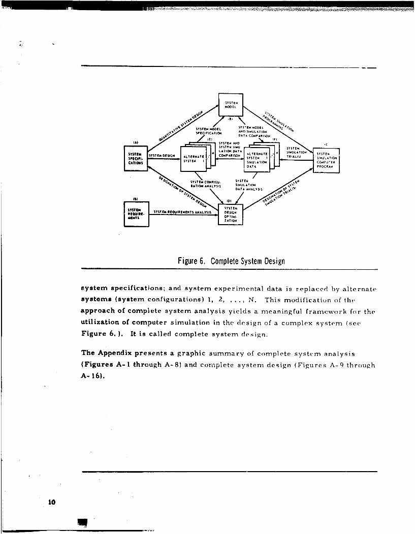
Figure 6. Complete System Design
system specifications; and system experimental data is replacced by alternate
systems (system configurations) 1, 2, ... , N. This modification of the
approach of complete system analysis yields a meaningful framework for the
utilization of computer simulation in the design of a complex system (see
Figure 6,). It is called complete system design.
The Appendix presents a graphic summary of complete system analysis
(Figures A-I through A-8) and complete system design (Figures A-9 through
A- 16).
10
, , n n n li s , , I I I I III li B nI 1 I I IIIII I I! 11III•IIIi~iiIIII!iII
QUANTITATIVE SYSTEM ANALYSIS
INTRODUCTION
A vast majority of knowledge in the physical sciences, and an increasing
amount in the behavioral and life sciences, is based upon models, of which
many are mathematical. Mathematical and statistical operations begin with
the assumption or existence of these models. To the author's knowledge,
relatively little comprehensive and definitive work has been published on the
modus operandi of their construction; even less has been published on con-
struction for systems with elements which are inherently qualitative, rather
than quantitative. Model construction is more an art than a science.
System analysis could accomplish part of the model construction by providing
a structure for the system. However, it remains for quantitative system
analysis to complete the mnodel construction by trauisforming qualitative
system elements into numerical form, and by specifying relationships among
,:omponent parts of the system. Quantitative system analysis, although in
somewhat preliminary form at present, is a comprehensive and definitive
approach to the modus operandi of model construction.
A summary of quantitative system analysis has been given in the discussion
of complete system analysis. It is described here in more detail.
Reftr'ences I and 2 contain an informative cxamplu of the application of
quantitative system analysis to the flow of scientific and technical information
(flow process). This application is summarized by Reference 1 and is pre-
sented in full by Reference 2. It is briefly introduced below. Pertinent
tables from Reference 2 illustrate the description which follows.
The Department of Defense (DOD) has sponsored the DOD User-Needs Study
to investigate, by means of a survey, the flow process within DOD (Phase I)
11
and the defense industry (Phase I1). Phase II surveyed a representative
sample of 1, 500 from a population of approximately 120, 000 engineers,
scientists and technical personnel. These personnel were employed by 73
companies, 8 research institutes and 2 universities that are defense
contractors.
An Interview Guide was employed to monitor the flow process by means of
questions exploring the component parts of that process. Sixty-three ques-
tions were asked regarding the USER of scientific and technical information,
his most recent scientific or technical TASK, his general UTILIZATION of
information centers and services, and the SEARCH AND ACQUISITION pro-
cess for information specifically related to the task. Responses to 55 of
these questions are qualitative.
The components of the flow process are USER, TASK, UTILIZATION, and
SEARCH AND ACQUISITION. Questions are the component parts, and
question responses are the elements.
The two major parts in the description of quantitative system analysis are
(1) transformation of qualitative system elements into numerical form, and
(2) construction of a model for relationships among system component parts.
The former contains development of a detailed structure for the system, and
definition of a numerical description for the detailed structure; the latter
contains development of a general structure for the system, combination of
related component parts in the general structure, and specification of a
system model for relationships among component parts.
TRANSFORMATION OF SYSTEM ELEMENTS
As noted above, the transformation of qualitative system elements into
numerical form is performed by the develorment of a detailed structure and
the definition of a numerical description for that detailed structure.
12
D)evelopmnent of a Detailed Structure
A detailed structure for qualitattive system elt_,niejnt.• 1s (lt(\ loped to sc rvyas the basis for the transform;ition of these eec mneOt In ,i lwli t ion, tI V,
detailed structure brings the locVil ;tspect.s of the systerm into focus :tnd
provides it foundation for a general structure. This det-ijiled structure is
formed by an informative arrangement of elerments-.
The first step is to specify a primary unifying charcteristic of the
elements in a component part. This element characteristic should be deter-
mined from not only the elements themselves, but also the function of the
component part.
The next ,.tep is to collect into groups those elements which are related by
the element characteristic. According to this characteristic, an ordering is
then arranged for groups and, to the extent feasible, for elements within
groups. All elements in a component part may be arranged into one ordering
if all elements within each group may be arranged into an ordering. Accord-
ing to the element characteristic, an element or group of elements is more
similar to elements or groups of elements which are closer to it in the
arrangement, than to those farther away.
Depending on the irnaplications of the element characteristic, there ,-.e three
types of detailed structure:
1. Visible structure, explicitly implied by the element characteristic.
2. Partically visible structure, implicitly implied by the elementcharacteristic.
1. Invisible structure, not implied at all by the element characteristic.
A visible structure is obvious, and possesses no flexibility. A partially
visible structure is apparent, but possesses some flexibility. An invisible
structure must be inferred, and possesses considerable flexibility. The
position of elements in the arrangement is meaningful in a visible structure,
13
and indicative in a partially visible structure, but only descriptive in an
invisible structure.
Examples of visible, partially visible, and invisible structure in the flow
process application are given in Tables I through 3, respectively. For the
tables, arabic numerals in parentheses--(1), (2), and so forth--indicate the
ordering in the Interview Guide; while roman numerals--I, II, and so forth--
indicate the ordering in the corresponding detailed structure. The numerical
description scale is included in the tables.
Definition of a Numerical Description
When the detailed structure is developed, its numerical description is
appropriate. By associating a number with each ordered qualitative element,
the numerical description provides a more exact differentiation among the
elements within a component part: and it enables estimation of the system
model, which is composed of relationships among component parts. The
numerical description also represents the system in a form to which a large
variety of numerical techniques may be applied.
According to the elemnent characteristic, the base point (zero) for a
numerical scale is selected. With each element, there is associated a
numerical value corresponding to its relative distance from the base point.
To standardize the numerical description, a negative integer, zero or
positive integer is associated with each ordered qualitative element whenever
feasible. Zero is employed when it is meaningful to consider the element to
be null, and a negative integer is employed when it is meaningful to consider
the element as opposite in direction to most of the elements. Variable
spacing between the associated numbers indicates that the elements exhibit
variable similarity, or distance from each other, according to the element
characteristic. The same number is associated with two elements in a
component part if--and only if--the two elements are in the same group of
14
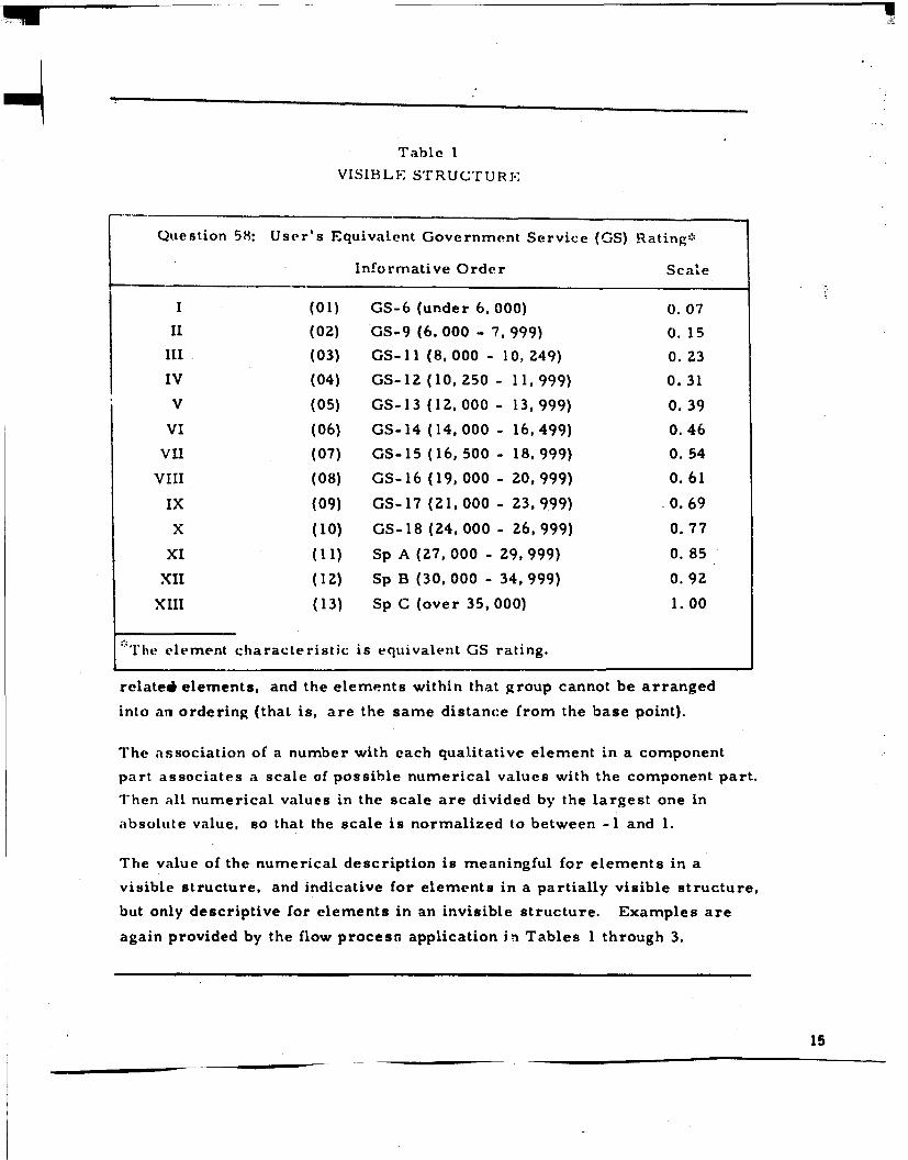
Table 1
VISIBLF STRUcTURE.
Question 58: User's Equivalent Government Service (GS) Rating:`
Informative Order Scale
1 (01) GS-6 (under 6,000) 0. 07
II (02) GS-9 (6, 000 - 7, 999) 0. 15
III (03) GS-11 (8, 000 - 10, 249) 0. 23
IV (04) GS-12 (10,250- 11,999) 0.31
V (05) GS-13 (12, 000 - 13,999) 0.39
VI (06) GS-14 (14,000 - 16,499) 0.46
VII (07) GS-15 (16, 500 - 18,999) 0.54
VIII (08) GS- 16 (19, 000 - 20,999) 0.61
IX (09) GS- 17 (Z1, 000 - 23, 999) .0.69
X (10) GS-18 (24, 000 - 26,999) 0.77
XI (11) Sp A (27,000 - 29,999) 0. 85
XII (12) Sp B (30,000 - 34,999) 0.92
XIII (13) Sp C (over 35,000) 1.00
::FThe element characteristic is equivalent GS rating.
related elements, and the elements within that group cannot be arranged
into an ordering (that is, are the same distance from the base point).
The association of a number with each qualitative element in a component
part associates a scale of possible numerical values with the component part.
Then all numerical values in the scale are divided by the largest one in
absolute value, so that the scale is normalized to between - 1 and 1.
The value of the numerical description is meaningful for elements in a
visible structure, and indicative for elements in a partially visible structure,
but only descriptive for elements in an invisible structure. Examples are
again provided by the flow process application in Tables 1 through 3.
15
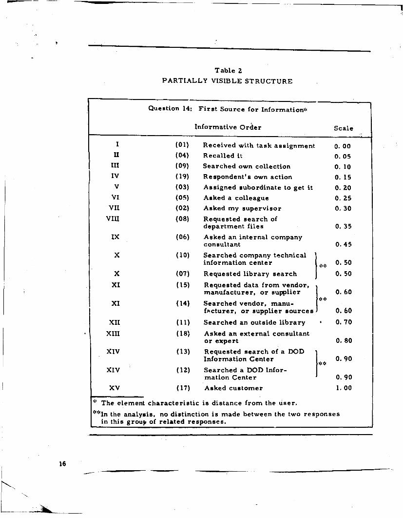
Table 2
PARTIALLY VISIBLE STRUCTURE
Question 14: First Source for Information*
Informative Order Scale
1 (01) Received with task assignment 0. 00
IU (04) Recalled it 0.05
III (09) Searched own collection 0. 10
IV (19) Respondent's own action 0. 15V (03) Assigned subordinate to get it 0. 20
VI (05) Asked a colleague 0. 25
VII (02) Asked my supervisor 0.30
VIII (08) Requested search ofdepartment files 0. 35
IX (06) Asked an internal companyconsultant 0.45
X (10) Searched company technicalinformation center 0. 50
X (07) Requested library search 0. 50
XI (15) Requested data from vendor,manufacturer, or supplier 0 0. 60I
XI (14) Searched vendor, manu-facturer, or supplier sources 0.60
XII (11) Searched an outside library , 0.70
XIII (18) Asked an external consultantor expert 0. 80
XIV (13) Requested search of a DODInformation Center 0.90
XIV (12) Searched a DOD Infor-mation Center 0.90
XV (17) Asked customer 1.00
SThe element characteristic is distance from the user.**In the analysis, no distinction is made between the two responses
in this group of related responses.
16
S.. .. ..
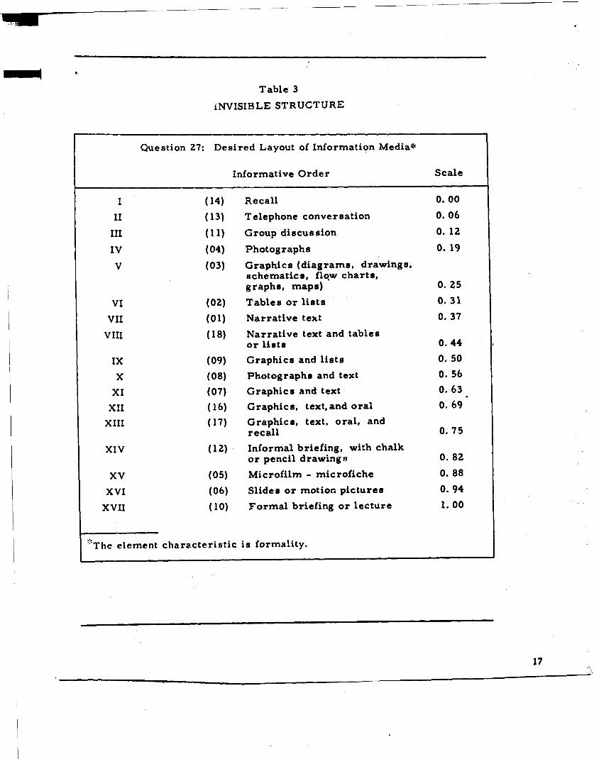
Table 3
iNVISIBLE STRUCTURE
Question 27: Desired Layout of Information Media*
Informative Order Scale
I (14) Recall 0.00
II (13) Telephone conversation 0.06
III (11) Group discussion 0. 12
IV (04) Photographs 0. 19
V (03) Graphics (diagrams, drawings,schematics, flow charts,graphs, maps) 0. 25
VI (02) Tables or lists 0.31
VII (01) Narrative text 0.37
VIII (18) Narrative text and tablesor lists 0.44
IX (09) Graphics and lists 0. 50
X (08) Photographs and text 0. 56
XI (07) Graphics and text 0. 63
XII (16) Graphics, text,and oral 0.69
XIII (17) Graphics, text, oral, andrecall 0. 75
XIV (12) Informal briefing, with chalkor pencil drawing" 0. 8z
XV (05) Microfilm - microfiche 0. 88
XVI (06) Slides or motion pictures 0.94
XVII (10) Formal briefing or lecture 1. 00
"The element characteristic is formality.
17
A detailed structure suggests its ow, tr,ý ntirica[ descrip' 10: w eni lie
elements in a component part have been prope-rly arranged. For i more
refined analysis, a numerical description could be tltered to i, n -orve the
linearity of important relationships whic l involve the corrre 's!po(l no
component part.
CONSTRUCTION OF A SYSTKIM MODPL
Development of a general structure, comnbinattion of r.late.d cuomponent parst
in the generai structure, and specification of at system rfnodel for relation-
ships among combinations of component parts in the general st ructLre
accomplish the construction of a system model.
Development of a General Structure
A general structure now is developed to serve as the basis for the construc-
tion of a system midel for relation ships ami-nong component parts, and
to bring the global aspects of the system into focus. This general structure
is formed by an informative and unifying arrangement of component parts.
The first step is to identify the components of the sytem. The next step
is to form groups of related component parts within components. Then an
ordering is arranged for components, groups within components, and
component parts within groups. To the extent feasible, the arrangement
should possess the desirable characteristic that a component part tends to
influence only those component parts which follow it.
An example is provided by the flow process application in Table 4, which
also includes component part combinations and linear relationships. In
this table, Q denotes Question; and 0 I 3 1 ..... 36 symbolize general
unspecified constants in the relationships. For simplicity, the same
symbols, P0 0, %, .... P are used in each relationship; although they
are not meant to denote the same constants.
38-- m--- ---
-- MOM
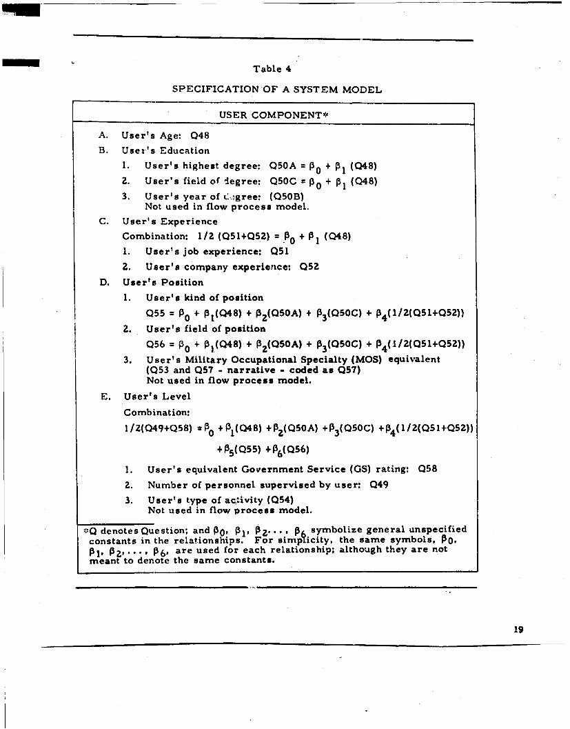
Table 4
SPECIFICATION OF A SYSTEM MODEL
USER COMPONENT*
A. User's Age: 048
B. User's Education
1. User's highest degree: Q50A = P0 + P, (048)
2. User's field of degree: Q50C = P0 + P, (Q48)
3. User's year of L.,gree: (Q50B)Not used in flow process model.
C. User's Experience
Combination: 1/2 (Q51+Q5Z) = 0 + PI (048)
1. User's job experience: 051
2. User's company experience: Q52
D. User's Position
1. User's kind of position
Q55 = P + PI(048) + P7(QSOA) + P3(Q50C) + P4(1/2(Q51+052))
2. User's field of position
Q56 = P0 + Pi.(048) + P3Z(Q50A) + P33(Q50C) + P4 (I/Z(Q51+Q52))
3. User's Military Occupational Specialty (MOS) equivalent(Q53 and Q57 - narrative - coded as 057)Not used in flow process model.
E. User's Level
Combination:
1/Z(Q49+Q58) =P0 + 1 3(Q48) +P?(Q5OA) +P3 (Q5OC) + P4(1/2(Q51+Q52))
+ P5(Q55) +1P6(056)
1. User's equivalent Government Service (GS) rating: Q58
2. Number of personnel supervised by user: 049
3. User's type of acctivity (Q54)Not used in flow process model.
:'.Q denotes Question; and Po0, Pi, •Z''", 7. symbolize general unspecifiedconstants in the relationships. For simplicity, the same symbols, P0,01, P2, .,., P36, are used for each relationship; although they are notmeant to denote the same constants.
19
mI
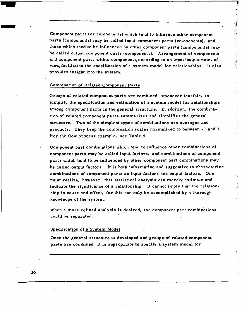
Component parts (or components) which tend to influence other component
parts (components) may be called input component parts (co~nponents), and
those which tend to be influenced by other component parts (components) may
be called output component parts (components). Arrangement of components
and component parts within components, according to an input/output point of
view, facilitates the specification of a system model for relationships. It also
provides insight into the system.
Combination of Related Component Parts
Groups of related component parts are combined, whenever feasible, to
simplify the specification and estimation of a system model for relationships
among component parts in the general structure. In addition, the combina-
tion of related component parts summarizes and simplifies the general
structure. Two of the simplest types of combinations are averages and
products. They keep the combination scales normalized to between -1 and 1.
For the flow process example, see Table 4.
Component part combinations which tend to influence other combinations of
component parts may be called input factors, and combinations of component
parts which tend to be influenced by other component part combinations may
be called output factors. It is both informative and suggestive to characterize
combinations of component parts as input factors and output factors. One
must realize, however, that statistical analysis can merely estimate and
indicate the significance of a relationship. It cannot imply that the relation-
ship is cause and effect, for this can only be accomplished by a thorough
knowledge of the system.
When a more refined analysis is desired, the component part combinations
could be separated.
Specification of a System Model
Once the general structure is developed and groups of related component
parts are combined, it is appropriate to specify a system model for
20
relationships among combinations of component parts in the general structure.
The terms, combination of component parts and component part combination,
also are used to cover the degenerate case of a single component part (for
example, Q56 in Table 4). A linear relationship among component part com-
binations is a mathematical expression of the variation in a given combination
of component parts (Y) as a linear function, with unspecified constants, of the
variations in the other component part combinations (X 1 , X?,...., Xp).
p
Analysis of the general structure from an input/output point of view yieldsthose component part combinations which are judged to be potentially relatedto each combination of component parts in the gener~l structure. Only the
potentially related component part combinations are included in the relation-
ship for that combination of component parts. It is frequently both convenient
and sufficiently accurate (for example, during exploratory research) to let
the system model be composed of linear relationships. An example is pro-
vided by the now process application in Table 4.
When the component parts have been properly -arranged, a general structure
suggests the relationships. A more refined analysis could specify additional
relatiornships, particularly those necessitated by the separation of component
part cornbknations.
21
COMPUTER SIMULATION
INTRODUCTION
Several classes of system problems, such as those where either subsystem
resource allocation or subsystem dynamic interactions are to be evaluated,
are not amenable to closed-form mathematical solutions. However, models
for such system problems have been created, reduced to computer algorithm,
and computed, providing important analytical results for systems engineers.
The technique employed is generally referred to as discrete simulation,
event simulation, or process simulation. This discussion will shed light on
the rationale and the steps involved, and will present computer aids for per-
forming such simulations.
SYSTEMS ENGINEERING ANALYSIS
Engineers are system-oriented people. Most of us operate with systems
where relationships between elements of the system (that is, the subsystems)
are readily stated in mathematical form. Solutions to our analytical problems
require that, at worst, we hire a statistician, who hires a programmer, who
hires a numerical analyst to develop an algorithm that provides the signifi-
cant figures required in computing the mathematical model of our system.
At best, we write our own FORTRAN program using library routines to con-
struct the system model and have the answer within a week.
For some engineers, however, systems become complicated and the models
do not lend themselves to easy assembly for computation. The elements
themselves may be tractable, but put together and encapsulated in the bigger
black box by procedures, priorities and operational constraints at a higher
system level than considered during element (subsystem) analysis, we find
23
ourselves in a less quantifiable, less well-ordered, less closed-form model
domain. This situation reduces our ability to predict with a high degree of
confidence system performance within expected ranges of operational param-
eters. Thus, systems engineering analysis proceeds with system model
assumptions (examples being linearity of constraints or static representation
of dynamic, time-phased subsystem considerations) that provide approximate
results.
Discrete system simulation can be used when one cannot find other techniques
for analyzing and evaluating alternative dynamic system operational schemes.
That is, the model can be built with which to experiment with controlled sys-tem variables in order to apply unusual stresses beyond normal system
operating ranges; or to force uncontrolled variables to such levels and for
such assumed periods of time that would either be too damaging or would take
too long in the real system operation, if that system actually exists.
Furthermore, we can formulate subsystem interactions between functional
elements of the system and relate these logically to the whole system. Such
submodel formulation relieves the systems engineer of the detailed task of
describing complete, closed-form system performance; however, he syn-
thesizes the complete system model by combining submodel formulation
provided by subsystem experts.
LEVELS OF SIMULATION ANALYSIS
Just where does simulation fit into a total system program? We can enumer-
ate four distinct periods or phases in the life cycle of a system: (1) research,
(2) development, (3) operation, and (4) replacement. In at least the first
three, various levels of uncertainty becloud the major aspects of the tasks
involved in accomplishing objectives. For example, in the research phase,
great uncertainty often surrounds the very concept of system proposals.
During the development of a system, many important design parameters
affecting system performance present alternative means of accomplishment.
In the operational phase, there are uncertainties concerning system growth
24
and flexibility. In all of these phases, system simulation is capable of
providing program managers with analytical guidelines for selecting preferred
system alternatives.
Re1search
System research takes the form of advances in technology along many lines.
Component development, automatic progran-iming of central compu1ters,
advanced display techniques, and responsive man-machine information query
subsystems are examples of related developments upon which advances in
system application depend. When research culminates, the existing system
concepts are based either on the unique application of the advanced technol-
ogy, or on revised concepts of data acquiisition, processing, display, or
management.
With success of the hypothesized system depending possibly on a yet unrealized
breakthrough in some technology area, how can the conceptualized system's
feasibility be demonstrated? Simulation can help predict the chance of
achieving successful implementation of the concept. In effect, the concept is
simulated to ascertain the feasibility of the following:
1. Reaction times required by system elements.
2. Proposed subsystem transfer functions.
3. Information content required for decision making.
4. Survivability characteristics in a hostile environment.
5. Phasing and planning compatibility.
6. Reliability goals.
The questions of concept answerable through simulation are broadly stated,
looking to total system reactions to subsystem stimuli, using engineering
estimates of the performance characteristics and other planning factors.
Estimates of subsystem performance are probabilistically stated, usually,
but are they consistent? Inconsistencies in planning factors conceived by
different segments of an organization responsible for pieces of the concept
25
are soon shaken out by a system simulation exercise performed early in the
research phase.
Development
In the development phase of the system life cycle, simulation provides
valuable insights into four major aspects of the design process: (1) alterna-
tive configurations, (Z.) allocation of funds for total system improvement,
(3) costs versus system effectiveness, and (4) policy changes versus system
performance.
Once system development has begun, and plans are beginning to yield'products,
the system can be further analyzed by simulation. At this stage of the sys-
tem life cycle, much more is known about the specifications of the subsystems.
Probability distributions and parameters associated with variables are better
quantifiable. The questions asked of the simulation analysis become more
specific: What priority should this sensor data have as opposed to all others?
How much data delay can be tolerated and still achieve effective system
operation? What is the effect of better equipment maint'enance policy (and
increased mean time between failures) on system performance? What are
the costs of Configuration A as opposed to Configuration B? What are the
gains in performance between System A and System B? Where are the
decision bottlenecks? What action best relieves bottleneck conditions? Do
we want to relieve these bottleneck conditions?
The process of designing subsystems of a system accelerates during the
development phase. Their elements and characteristics can be either
described in great detail or may be estimated very confidently. Some of these
characteristics, such as subsystem data transfer capacity, become critical
with respect to the potential stress that the system will undergo. Detailed
descriptions cf these critical characteristics are parameterized in the sys-
tem model during the development phase of system design. System perform-
ance can be examined while these elemental values are allowed to vary. A
preferred combination of system policy and hardware characteristics can be
26
established from simulation analysis cf several choices, measured by values
of the chosen objective function.
Operation
There are many impelling reasons for simulating an operational system.
These fall into the following categories: (1) system capacity limitations
versus stress levels, (Z) decision automation potential, (3) total system
value analysis of subsystem improvement, and (4) off-line training exercises.
In the operational phase of a system's life, all of the data about all of the
elements of each subsystem can be collected to any degree of refinement.
Certainly, a computer system simulation model could not be built with more
realism than ex..ists in the actual system. However, computer simulation
still plays an important analytic role in extending understanding of existing
systems. At this stage, questions of analysis are more precisely directed
to known system elements. The systems engineer asks: what is the effect
on system performance of sampling sensor data at less frequent intervals, if
the basic error rate frequency distribution of the sample data does not
change? If present operational activity were suddenly to increase by 20%,
which subsystem element would be the first to break down? Or if increased
by 50%, or doubled? If man-made decisions were programmed into hardware,
what would be the expected incidence of inappropriate system response?
With normal system growth, what is the approximate time that present sys-
tem elements would use up existing excess capacity? How can we best cope
with these anticipated problems--better procedures? Better hardware?
More hardware?
Summary
Simulation fits into the system analysis picture wherever uncertainty and the
effects of the time dimension or the interrelationship of different elements
within a system need to be better understood, and a system field experiment
or exercise is too costly or impractical. Also, because the nature of complex
27
systems operation is known only probabilistically, the effect of random
variation requires a dynamic simulation in order to examine interactions
between and among subsystems.
DISCRETE SIMULATION FOR SYSTEM ANALYSIS
Developments in computer technology have broadened the scorpe of large,
complex systems synthesis. Computers have grown in storage capacitiesand have increased in speeds; software designed for simulation problems
now include discrete simulation systems packages; and statistical design
techniques have been coupled with simulation for more effective systems
analysis.
Engineers, in exploiting these new computer simulation developments, are
now confronted with the necessity of understanding discrete simulation
principles and techniques. Foremost in the analytical process is a require-
ment to structure system models that can be efficiently computerized.
Engineers and computer model builders must share the burden of discrete
simulation modeling.
By assuming that a system is organized as definable and important subsystems,
and that relationships among these subsystems can be either formulated or
described by logical conditional procedu.-es, a basis exists for model building.
To attain a feasible basis for modeling a system, specific goals--or system
objectives that the system must satisfy--must be established. To achieve a
realistic system model, all necessary and interesting system elements and
relationships must be quantifiable, and the objective functions established to
measure performance of examined system structures (that is, how well each
structure achieves system goals).
System Objectives
Starting with the assumption that the system exists (even conceptually), the
first step in system model building is to establish system objectives.
Analysis requirements, and the structure of a simulation model, clearly
28
should be guided by these objectives. In simulation model-building terms,
this r.aeans: list the questions to which the engineer wishes quantified answers
about system performance. Prociteding from defined objectives, the engineer
can develop functional block diagrams and stimulus-response lines between
system elements necessary for driving all activity within the system. These
diagrams help the model builder describe the constraints in the system, the
possible system states produced, and the probability of achieving each state.
Stimuli exogenous to the system must also be identified.
Selecting System Variables
With the aid of a computer model builder, and with established system
objectives as a guide, key variables of system performance will be identified.
They will be either controlled or uncontrolled with respect to the system.
An objective function will be developed, expressed in terms of these variables.
This is the model builder's way of computing system performance measures
for objective comparisons among different structures of a system. Require-
ments will be established for data and for estimates of input-output functions
(submodels) characterizing subsystem interactions. Descriptions of all
attainable system states and the subsystem activities that produce each state
complete the system description for model building.
Events of a Discrete Simulation
Decomposition of a system's operation into component steps that may
(stochastically) or do (determi stically) change status of key system variables
produces: (1) a list of system events, and (2) cause-and-effect expressions--
equation, logical algorithm, and so forth--relating dependent and independent
variables of each event, to describe the reasons that changes occur.
These events are the conditions modeled in a discrete simulation analysis.
That is, the moment of change is modeled, and total system effect of that
change is evaluated in a simulation of these moments. Between events,
because the system is quiescent, performing normally without status change,
29
or undergoing discrete changes, only the independent variable time will
change state. By definition, both the start and the end of a system operation
step become events of a discrete simulation model.
The mathematics of each event describes independent variables whose values
or states lead to possible alternatives of the dependent variable state. An
isolated event is one in which dependent variables are not independent
variables of other events that could occur simultaneously. By considering
time and space as criteria and by reducing either or both of these reference
bases, almost all system events can be ultimately defined as isolated. This
essentially increases both the detail required to describe the outcome of an
event and the number of events required to describe system dynamics. If
sequential operations occur at different time frames and affect different
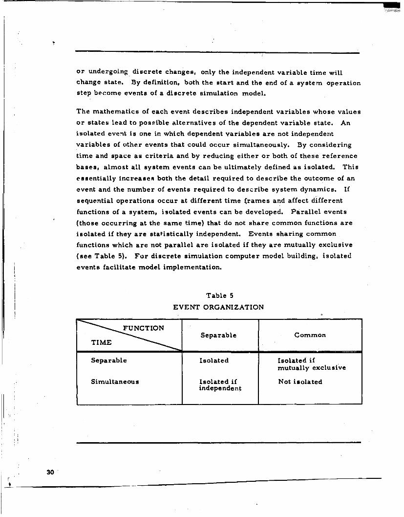
functions of a system, isolated events can be developed. Parallel events
(those occurring at the same time) that do not share common functions are
isolated if they are statistically independent. Events sharing common
functions which are not parallel are isolated if they are mutually exclusive
(see Table 5). For discrete simulation computer model building, isolated
events facilitate model implementation.
Table 5
EVENT ORGANIZATION
Separable CommonTIME
Separable Isolated Isolated ifmutually exclu sive
Simultaneous Isolated if Not isolatedindependent
30
b@
Formulation for Simulation
A system model is formulated for discrete simulation by logically or
mathematically describing events and associated variables. Events describe
system actions which change the state of the system (that is, change' variables
of the system). Variables are the entities of the system whose character-
* istics, when quantified, provide state conditions whose change must be
recognized in the simulation. The numeric values of these characteristics
become vectors or arrays of state condition.
Variables that confront mode' ,,lders are either controlled or uncontrolled
in the system and its operating environment. 'ncontrolled variables in the
system are controllable in a simulation, possibly by probabilistic algor-
Sithms. Y, Some simulations will not control all controllable variables, if
certain of these factors are not interesting at the moment; if experimental
design dictates they need not be measured explicitly; or if they are included
only to provide richness to a model (that is, provide a "realistic" model).
These are generally treated as random variables.
Several computer languages are available at present to implement system
simulation models. The need for specific attention to discrete simulation
software that eases the burden of programming, coding and debugging sys-
tem models is obvious when past history of project elapsed times is reviewed.
No such review will be made here; rather, we will summarize some of the
model building conveniences available for discrete simulation. These are
recognized as beneficial to other classes of computer programs, but several
simulation-specific systems have organized and exploited these techniques.
Significant reductions of elapsed times, from system modeling to operating
simulation programs, have resulted.
This is one of the compelling reasons that simulation experiments are
preferable either to field tests or experiments with actual systems.
31
Timing
A unique requirement for simulation systems is to organize the managementof time passing as events occur. Time is an independent variable of all
simulations. Good techniques to simulate time can both increase analysis
accuracy and reduce computer operating time. If simulation start time is
T and progression over time is Ti, T 2 . .. Tk..., then time in simulation
must be monotonic increasing in (k). A model must simulate all events (i),
and each occurrence (j) of event (i) at time Tm (E. m) before those at T ifm itj n
m<n; otherwise, a cascade of system interactions triggered by the dependent
variables of E m i = 1, 2,...; j = 1, 2... that may be independent variablesn i, i
of En . will be disregarded, or, worse, erroneously simulated. "
Constraints determined by the systems engineer are used to compute modelelapsed time within each event. This could be a function of system overall
status at any point in a system operating cycle, of stochastic parameters,
etc. Caiendars of events are maintained by the simulation software, and each
event is se,-uenced to occur in order of time preference, however determined
in the model. Describing how elapsed time between system status changes will
occur as event constraints is sufficient to allow software to sequence properly
all events to determine realistically the effect of time on system performance.
Entity Descriptions
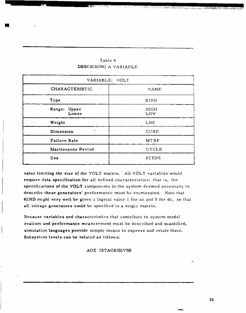
Simulation languages employ mathematical notation and easily understood
English expressions to describe variables and their characteristics. For
example, a voltage generator that is part of an automatic checkout device
might be labeled VOLT and described as in Table 6. Reference to the cube
of the voltage regulator could be stated in the program as CUBE (VOLT). If
there are several different generators of this type, then the variable VOLT
could be labeled VOLT = MANY and the quantity "MANY" be given a numeric
"**The problem of interactions between and among events occurring at Tksimultaneously is ignored.
32
'Fable 6
DESCRIBING A VARIABLE
VARIABLE: VOLT
CHARACTERISTIC NAME
Type KIND
Range: Upper HIGHLower LOW
Weight LBS
Dimension CUBE
Failure Rate MTBF
Maintenance Period CYCLE
Use STEPS
value limiting the size of the VOLT matrix. All VOLT variables would
require data specification for all defined characteristics; that is, the
specifications of the VOLT components in the system deemed necessary to
describe these generators' performance must be enumerated. Note that
KIND might very well be given a logical value 1 for ac and 0 for dc, so that
all voltage generators could be specified in a single matrix.
Because variables and characteristics that contribute to system model
realism and performance measurement must be described and quantified,
simulation languages provide simple means to express and relate them.
Subsystem levels can be related as follows:
AGE (STAGE(SIVB))
33
to specify a type of a-tomatic equipment (AGE) specifically used for a
particular stage (STAGE) of the Saturn S-IVB (SIVB). Furthermore, the
expression
COUNT (STAGE, SIVB (PLACE, STATE))
might be countdown time accumulated for each stage of several S-IVB's at
different launch complexes and in different conditions with respect to a total
countdown cycle.
Event Computations
Simulation languages not only permit direct and English-like statements that
establish system variables and attributes, but.event computations are also
made with the following statements:
IF HIGH (VOLT)- LOW (VOLT) GR 1Z5, THEN DO....
FAIL = EXP**RANDM*MTBF (VOLT)
Association of items into classes containing commton characterittles It
accomplished with set instructions. Arithmetic and logical operations can be
performed on all variables temporarily grouped into sets by the dynamics of
systerr. performance. For example, queues of items awaiting future failure
computed on the basis of mean-time-to-failure can be gathered in a system
factor called QUEUE, automatically ranked on the earliest time to anticipated
failure. Operations that examine or change sets are perfori id on the factor
QUEUE. Simulation languages, not the model builders, worry about the
bookkeeping needed to manage the fluctuating size of QUEUE.
Other common set organization procedures, such as LIFO and FIFO, are
automatically controlled by the languages after the model builder specifies a
rule. Usually, he specifies such set discipline by a simple mark on a data
input form.
34
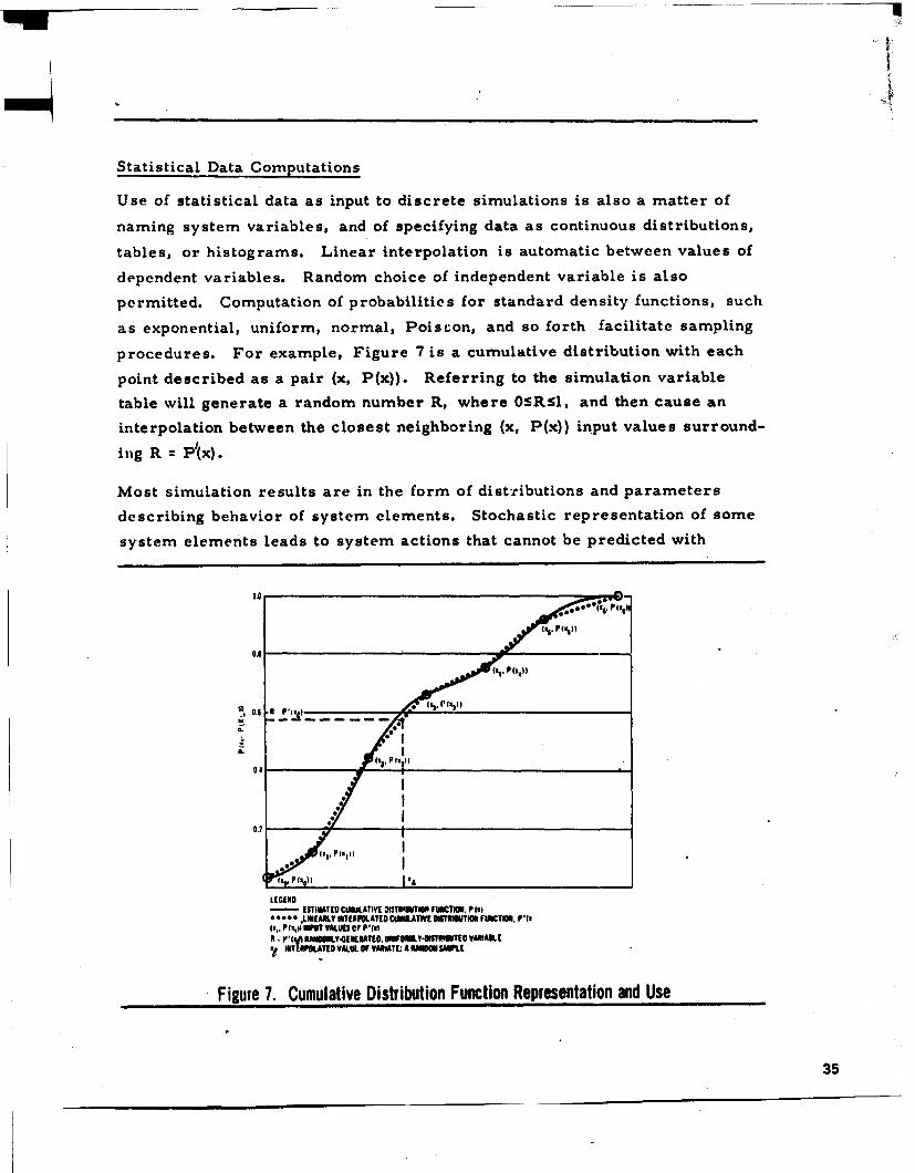
Statistical Data Computations
Use of statistical data as input to discrete simulations is also a matter of
naming system variables, and of specifying data as continuous distributions,
tables, or histograms. Linear interpolation is automatic between values of
dependent variables. Random choice of independent variable is also
permitted. Computation of probabilities for standard density functions, such
as exponential, uniform, normal, Poisron, and so forth facilitate sampling
procedures. For example, Figure 7 is a cumulative distribution with each
point described as a pair (x, P(x)). Referring to the simulation variable
table will generate a random number R, where OR-l:., and then cause an
interpolation between the closest neighboring (x, P(x)) input values surround-
ing R :VP'(x).
Most simulation results are in the form of distc'ibutions and parameters
describing behavior of system elements. Stochastic representation of some
system elements leads to system actions that cannot be predicted with
1.0
ros. P(Ei()
U4. P(44))
0.4 P-- -- -- -- --e. l
0. ? I
h P•Is. P45
- [STINmTD CUiULATIYE 3ISTNIOPT FUVCTIM. P(a)*LMlAiLY TICPPOLATIO CUMILATIVE STIOUTIOW FCTi. P'rx
(I, P t1i0 WUT VALUES OF Pl(o
#" -TOVAUEPAR0TI tIDmAeLC K't ~l~tA.[O U F VJUhAT[:A Offiem sP[
Figure 7. Cumulative Distribution Function Representation and Use
35
certainty. Thus, expected values, average lengths of waiting times, variances,
frequency distributions, and so forth, are typical forms of simulation results.
Simulation languages accomodate statistical data gathering. Simple instruc-
tions (macros) contain complete programs for integrating variables over
time, computing means, variances and other statistics, and compiling data
points for histogram and curve plots.
Closely associated with techniques used in simulation language to compile
statistical behavior of system variables is the facility to report these
statistics to the simulation analyst. Several current simulation languages
provide such data automatically; others allow analysts freedom to draw out-
put formats, designate the variable name (for example, VOLT), and map
with code marks specific data. Reports then are assembled in their entirety
by the simulation language according to the prescribed map.
Reference 3 presents an excellent discussion of computer simulation in
general.
SYNOPSIS
In practice, discrete simulation only partially fills the void in the process of
complete system anilysis, because one cannot hope to optimize system per-
formance with design parameters only through this process. This presenta-
tion, however, has shown how system engineering analysis can be better
organized to achieve more rational choices among alternatives by using
simulation. In fact, simulation use is proposed very early in the research
phase of the system life cycle. Further improvement of models possible in
the system development phase only enhances simulation applicability while
there is still time to alter design parameters. Even while systems are
operational, simulation is a technique that aids systems engineers to answer
redesign questions involving advanced procedures, revised operating policies
and unusual stress conditions.
36
This paper has also discussed system analysis approaches that insure better
models for discrete simulation. It is important that system engineers and
simulation model builders together attack system analysis and synthesis
problems to insure both feasible and realistic simulations. Finally, some of
the simulation language aids have been described that translate system models
into efficient discrate simulation computer programs.
v3.
SYSTEM OPTIMIZATION
INTRODUCTION
In the context of this paper, a major purpose of a complete system analysis
is to improve, in some sense, the system or its output. From the viewpoint
of the systems engineer or the operations analyst, this improvement is
accomplished through an optimization process. Thus, optimization is the
process of improving a system with "the best" as a goal.
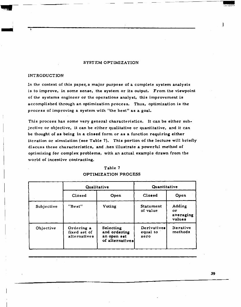
This process has some very general characteristics. It can be either sub-
jective or objective, it can be either qualitative or quantitative, and it can
be thought of as being in a closed form or as a function requiring either
iteration or simulation (see Table 7). This portion of the lecture will briefly
discuss these characteristics, and .hen illustrate a powerful method of
optimizing for complex problems, with an actual example drawn from the
world of incentive contracting.
Table 7
OPTIMIZATION PROCESS
Qualitative Quantitative
Closed Open Closed Open
Subjective "Best" Voting Statement Addingof value or
averagingvalues
Objective Ordering a Selecting Derivatives Iterativefixed set of and ordering equal to methodsalternatives an open set zero
of alte rnative s
39
OPTIMIZATION METHODS
Subjective-qualitative, or nonquantitative, methods include the following:
(1) authoritative statements that this system is the "best" without proof or
justification- -the "salesman approach"; (Z) asking others for their opinion--
the "expert judgment approach"; and (3) voting in a committee--the "demo-
cratic approach". Many system decisions, if not most, are made by these
techniques.
Subjective-quantitative methods include (1) the calculation of a numerical
value for some system characteristic for one configuration and saying, "it
only costs this much" or "it's blue isn't it?"; (Z) comparison of this value
with others, especially competing, systems such as "this car is cheaper than
Z6 models of the so-called low-priced three"; and (3) "the weighted average
cost of operation is x cents per ton mile, " where neither the method of
weighting nor the factors averaged are made explicit.
Objective-qualitative methods include (1) the ordering of a fixed set of
alternative configurations-- "the best tactical fixed wing aircraft for this job
is--" and (Z) the ordering of an open set of alternative configurations-- "the
best solution to this tactical problem is to use a--, " when all feasible equip-
ment items are considered.
Objective-quantitative methods (for each independent measure of effiectiveness)
include the following:
1. Compute the measure for each possible configuration and select theone with the highest (or lowest) value.
2. Compute the measure for some alternatives, plot the measure forthe principle variables, and select the "best" by inspection of theresulting curves.
3. State the measure as an equation (function of controllable variablesand parameters).
40
N o w n - ,_,_,_...... . .. .. ..
A. If the furction is differentiable, !heri L!ie solution may bc
obtainable in closed form by setting the partial derivativesequal to zero and solving, or through the uise of La Grin~gianmultipliers.
B. If the function is not differena-le, ,r : ae D±rtL:als are c ir.-
plex and awkward, the nroce(.r•r 's *, - , >. rno 'iterative method.
(1) Interpolation methods (Newtor.'s Method).
(Z) Linear programming.
(3) Quadratic programming.
(4) Dynamic programming.
(5) Non-linear programming.
(a) Steepest ascent based on local partial derivatives.
(b) Pure search methods.
"41
INCENTIVE CONTRACTING EXAMPLE
In the contracting world, the basic problem is that of maximizing the fee
earned as a function of the risk involved. Contracts usually call for thedelivery of a number of items of a specified quality in a specified time
period at a specified cost. The questions of risk and uncertainty arise in
estimating the cost, quality or delivery schedule, or all three. If this
uncertainty is small, contract terms probably should specify a fixed price
(FP). This, in effect, makes the contractor assume all the risk, and in
return permits him to make and keep any or all fees (price minus actual
cost). On the other hand if this uncertainty is large, the customer may have
to assume the risk in order to get a contractor to agree to do the work. Inthis case,a cost-plus-fixed-fee (CPFF) agreement is usually the best solution.
In the came of moderate risk, the contractor may be motivated to meet per-
formance requirements, schedules and cost estimates if his earned fee is
variable and also is dependent on how well he meets the customer's goals.
Thus the incentive contract was born: in its most basic form, it states that
the fee earned is a function of how well the contractor periorms.
To a systems engineer, this definition indicates that a mathematical function
can be developed which expresses the relationships among fee, cost, per-
formance and delivery time.
Fee = f (Cost, Performance, Time)
F = f(C, P, T)
It also suggests that if such an equation can be d&weloped, it can also be
optimized. For instance, should the customer suggest an incentive contract
in an RFP, it usually means that he has analyzed the work to be performed
in meeting the schedule and performance specifications, and has established
a set of- value judgments concerning the amount of additional fee he is willing
V
to pay to obtain higher performance values or earlier delivery dates. This
is most often construed by the contractor to mean penalties for poor per-
formance or late delivery. In any event the contractor must also analyze
the work to be performed, must estimate the uncertainties and risks involved,
and must establish the amount of fee he desires for various levels of cost,
performance and delivery times. The process of incentive contract negotia-
tion then becomes one of reaching a compromise between these two estimates.
The problem of estimating the risk is equivalent to that of estimating an
expected performance level, and establishing a confidence region around it
for each performance factor and schedule item. If this is done and the
relationships among the factors are known, the overall or total risk can be
estimated in cumulative probability distribution" form. To accomplish
this estimate it is necessary to establish a conceptual model, develop
a mathematical model within this framework, estimate the unknown parame-
ters, and finally solve for fee as a function of the selected factors and
parameters. In other words, a complete system analysis is performed.
The model chosen for this incentive contract is of the following form: earned
fee is a function of cost and performance, F = f (C, P) . This model was
chosen because of its simplicity and because it could be represented by a
three-dimenp'onal surface. The model was constrained further by reasoning
that the fee should decrease as cost increases, and should increase as
performance increases. Two further constraints were added for this
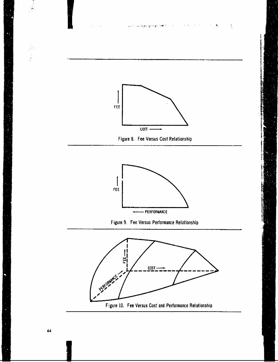
particular case. One, the relationship between fee and cost should be
piecewise linear, to correspond with the contractual concept of cost sharing
(see Figure 8).
The relationship between fee and performance should be quadratic, to
correspond to the belief that every increase in performance should be
rewarded with an increase in fee, but at a lower rate as performance
becomes higher (see Figure 9). The combination of these constraints results
in a three-dimensional model as illustrated in Figure. 10.
43
I 'V.1. •:-
FEE
COSTl-
Figure 8. Fee Versus Cost Relationship
FEE
- PERFORMANCE
Figure 9. Fee Versus Performance Relationship
- IL
Figure 10. Fee Versus Cost and Performance Relationship
44
14
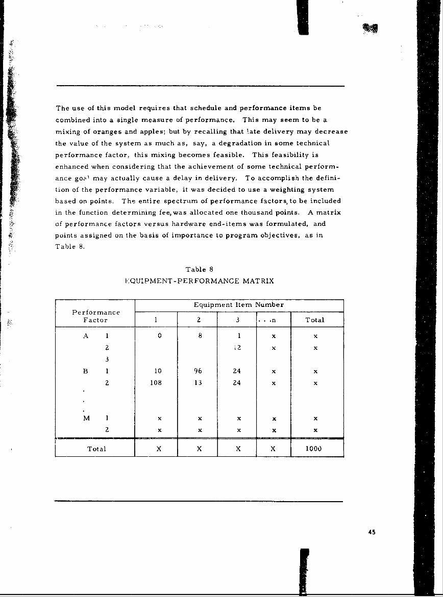
The use of this model requires that schedule and performance items be
combined into a single measure of performance. This may seem to be a
mixing of oranges and apples; but by recalling that 1ate delivery may decrease
the value of the system as much as, say, a degradation in some technical
performance factor, this mixing becomes feasible. This feasibility is
enhanced when considering that the achievement of some technical perform-
ance goal may actually cause a delay in delivery. To accomplish the defini-
tion of the performance variable, it was decided to use a weighting system
based on points. The entire spectrum of performance factors, to be included
in the function determining fee, was allocated one thousand points. A matrix
of performance factors versus hardware end-items was formulated, and
points assigned on the basis of importance to program objectives, as in
Table 8.
Table 8
EQUIPMENT-PERFORMANCE MATRIX
Equipment Item NumberPerformance
Factor 1 2 3 . • .n Total
A 1 0 8 1 x x
2 12 x x
3
B 1 10 96 24 x x
2 108 13 24 x x
M I x x x x x
2 x x x x x
Total X X X X 1000
45
This form of weighting is ideal in the sense that quantitative items such as
delivery date, dichotomous items such as test pass or fail, and subjective
items such as maintainability and flexibility, can be included in the same
scale. It also permits the negotiation of the relative value of each item,
separately or in combination. A review of these weights was made to avoid
the inadvertant over-weighting of any particular item due to interaction
effects. This so-called domino effect can be treated by assigning the points
in a manner to account for these interactions.
While the performance scale was being negotiated by teams of technical
experts representing both the customer and the contractor- -negotiation to
ensure that the customer's goals would be met and that the technical risks
would be shared--the cost experts took a look at the expected total costs of
the program. These negotiations produced an expected cost, called by the
contracts people target cost or administrative target cost, and a rough
estimate of the probability of overruns and underruns,of specified amounts i
or percents of target cost. These two separate but related efforts produced
a qualitative and highly subjective estimate of the expected performance and
cost points. One such estimate, made by the contractor in the particular
case in mind, was that the performance points achieved would be about 65G,
or 65% performance, at a cost equal to a 15% overrun (target cost plus 15%).
At the same time, the customer's estimate at this point was 80% performance
at a 10% over-run. Because these two estimates did not agree, negotiation
was required to settle the point.
The contractor justified his position by separately and independently esti-
mating the probability of making the points assigned to each cell in the
matrix, as shown in Table 8. Each estimate was made by the technical
person responsibie for doing the actual work. At the same time, an upper-
and lower-bound estimate was made. This was a subjective procedure
designed to correspond to the statistical procedure of establishing a confidence
interval. A review of these procedures by the negotiation teams produced a
46
negotiated position that the most probable performance and cost region fell
between 60% and 80% performance, and between 0% and 15% cost over-run.
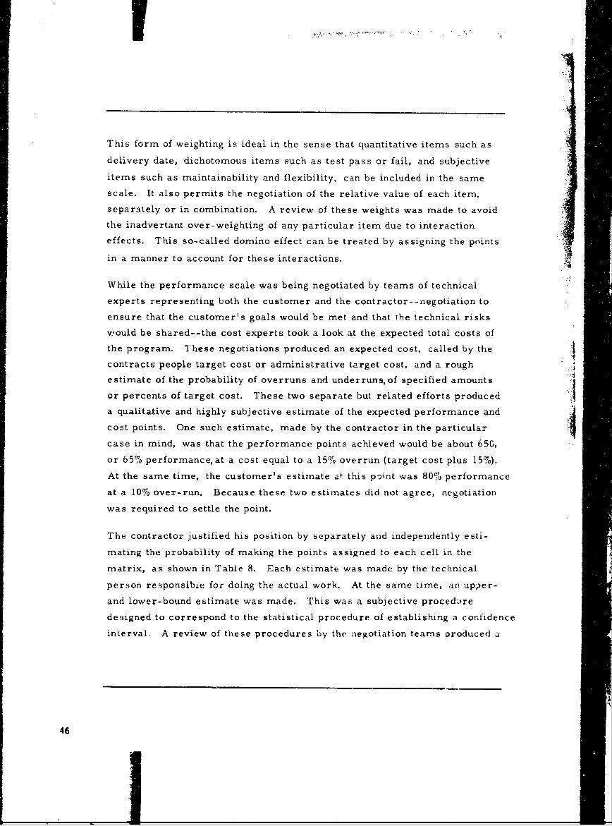
This agreement produced a most likely region for the model; but fee doliars
or percent had not been agreed to, so the exact location was still in doubt.
The next and final step in specifying the exact model (specification of the
unknown parameters) was accomplished by negotiating the fee dollars for
each corner of this region or box (s.e Figure 11).
100%
60%
T.C. COST
Figure 11. Negotiated Relationship
This negotiation took the form of establishing a set of dollar fees for each
of the four corners which was acceptable to both parties. Once this had been
accomplished, the shape of the model that would pass through these four
points was determined by negotiating the maximum fee dollars for 100% per-
forroance and minimum cost, and d set of share ratios. This maximum point
is very probably unobtainable, and was determined primarily by considering
the effect of such a point on the renegotiation board. This point :,nd a set of
share ratios were negotiated; the share ratios are for determining the portion
of any change in cost from the target cost to be borne by the customer and
the contractor. In turn, the exact rnathematical model was specified for this
contract.
Before the proposal was submitted by the contractor, a computer model was
developed for the general model which was piecewise linear in the -Lost-fee
47
SItI
plane, and quadratic in the fee-performance plane. This program was designed
ratios; and through curve-fitting techniques, solve for the quadratic coefficients
at each cost break (the point where cost-share ratio changes). These coeffi-
cients and cost-break values then completely defined the surface, and the 4quantitative aspects of the contract.
This col iputer program is, in effect, a simulation routine for determining
the effect of various combinations of cost and performance on fee. In addition,
the computer could and did compute such items as fee dollars per performance
point per cost dollar, so that tradeoffs betweei, 'ost and performance could be
investigated. This program was available during thc entire negotiation period,
and was used by both sides to determine the effect of each proposed change.
It was used to optimize the contract in the sense of assuring the customer a
high probability of obtaining his desired performance, cost and delivery
objectives, at the same time assuring the contractor that he would obtain a
fai• ri•arn for his effort.
For more detailed information on incentive contract negotiation, see Refer-
ences 4, 5 and 6.
Optimizing by use of a computer simulation of a mathematical model, to
provide estimates of system performance for systematically changed values
of the controllable variables and/or parameters, is probably the most
powerful optimizing technique available for the complete analysis of highly
complex systems. It is particularly appropriate in the conceptual develop-
ment phases of a la-rge system. When kept up to date with system design
changes and newly discovered relationships, it provides the most powerful
tool for managing and controlling the procurement phase, and assures that
the final sysLern meets its technical objectives on time and within an
acceptable cost range.
48
REFERENCES
I. A. F. Goodman. Flow of Scientific and Technical Information: TheResults of a Recent Major Investigation. McDonnell Douglas AstronauticsCompany - Westrn Division Paper DP-4516 (AD 657 558), RevisedSeptember 1968.
2. A. F. Goodman, J. D. Hodges, Jr., et a), Final Report, DOD User-Needs Study, Phase Ii: Flow of Scientific and Technical Informationwithin the Defense Industry, Volumes I, I1, and III. North AmericanRockwell Corporation - Autonetics Division Report C6-2442/030(AD 647 Ill AD 647 112, and AD 649 284), November 1966.
T. H. .aylor, J. C. Balintfy, et al. Computer Simulation Techniques.John Wiley and Sons, 1966.
4. NASA Incent :ve Centracting Guide, Second Edition. National Aeronauticsand pace Administration Report NPC 403, January 1965.
5. Final Report, Planned Interdependency Incentive Method. ManagementSystems Corporation Contract NAS9-3466, January 1965.
6. E. P. Durbin. Contingent Pricing Policies. Stanford University -Department of Statistics Technical Report 76, December 1964.
49

APPENDIX
COMPLETE SYSTEM ANALYSIS: A GRAPHIC SUMMARY
Figures A- 1 through A-8 graphically summarize complete system analysis,
and Figures A-9 through A- 16 graphically summarize complete system
design.
51
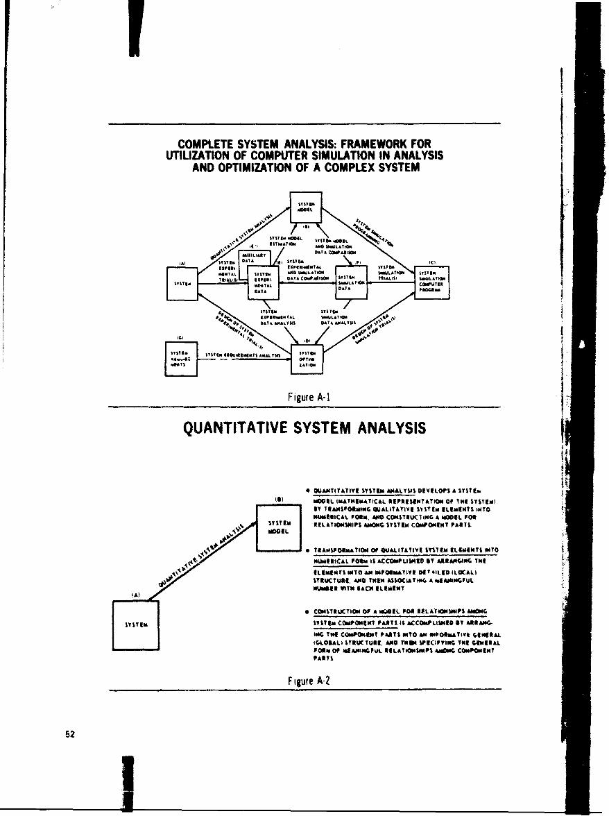
COMPLETE SYSTEM ANALYSIS: FRAMEWORK FORUTILIZATION OF COMPUTER SIMULATION IN ANALYSIS
AND OPTIMIZATION OF A COMPLEX SYSTEM
TgAL~~SI *Ig I T DAT A CPOWN DAT IflyiM TAL1 wau"
Figure TA* IVITtQUNTTAIV SYSLTEM0 ANUALY SSTIS
SOE LMATtNEMTCI IEUIITOM OPUY12 4 iYVu
SYITIM SEITSM P ~g~5$3~ OO11PSS
DA T1NFIs4a MAL WSAITTV DATAE ILENNISIN
1INRCA PO9ARAIN AKACgLPIEOVMT4US ~t-
QUANTIATIVESYST O AN IPIALYISE0111 LA
*UNITAUTUIVE SYSTE14M ANSIS C IA ILW6 A MI SM"P
&Ve~ VTRNSOMN QUA0 LEINTAIESST ELMNSNO
*CMi~tRUCAL ORM. AN CMSYUCIN PO MIAVODEL P041M
111 tm NUMTERIA F~ORM 1 PATIICCOMPLI0V IT ARAPV ~T AEE
% - IL t"M TH %~P4M PAIS510 A14IINVATI 56Of l E O CALV 6iw
iGL.O*ALl 1TIUCTUNE. AND TWNV SPECIFYING TWE CAMISALFORM OF MEANINGFUL uULATIOENSIPA AMONG CMP0MENT
Figure A-2
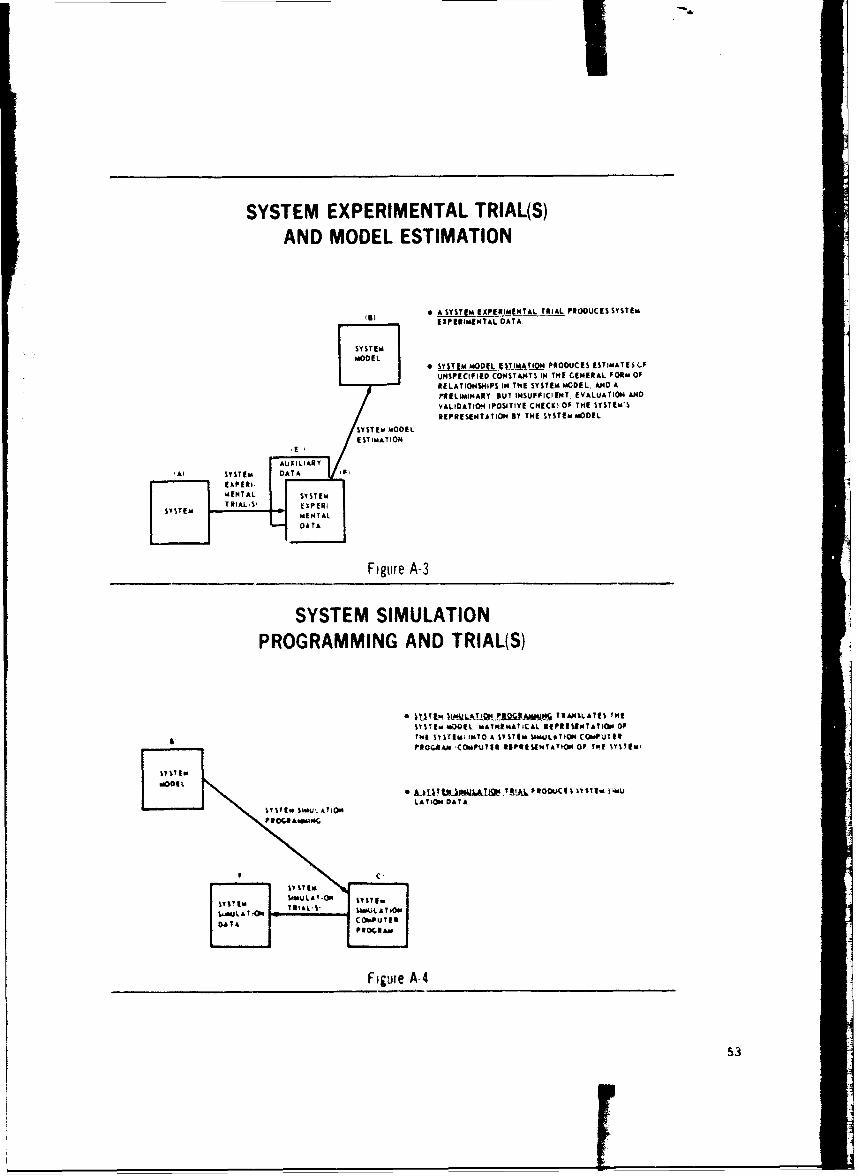
SYSTEM EXPERIMENTAL TRIAL(S)AND MODEL ESTIMATION
0 ASTgtEMEAPERIMEMTAL TRIAL PRODUCES SYSTEMEXPERIMENTAL DATA,
STYST EMMODEL
0 SYSTEM MODEL ESTIMATION PRODUJCES ESTIMATES (,FUNSPECIFIED CONSTANTS IN THE GENERAL FORM OF
RELATIONSHIPS IN TH E SY STEM MODE L. AND A1T1ELIMIMARY, BUT INSUFFICIENT, EVALUATION ANDVALIDATION (POSITIVE CHECW OF THE SYSTEM'S
REPRESENTATION By THE SYSTEM MODEL
SYSTEM MODELESTIMATION
'ASYTE SIMULATION, ip
META SYSTEMRNSATS H
SYSTEM MODELS IAIMATCI XPRIEMATON
DATAN AT
Figure A-3
SYSTE SIMUATIO
PROGRAMMINGArDTIAL(S
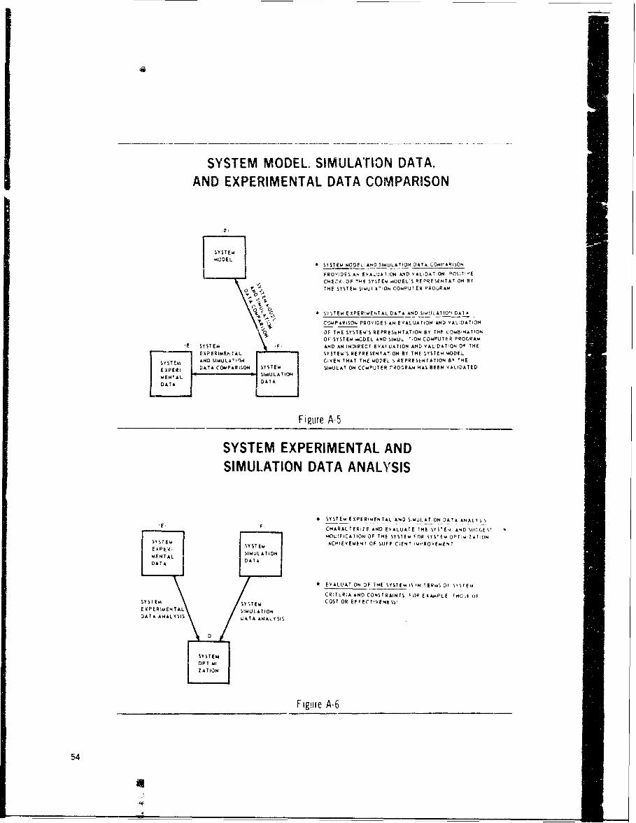
SYSTEM MODEL. SIMULATION DATA,AND EXPERIMENTAL DATA COMPARISON
SYSTEM._•. MODEL
M SYSTEM MODEL AND SIMULATION DATA COMPAINISON
PROVIDES AN EVALUATION AJND VALIDATION POS;TIlE
17CHECK, OF TVE SYSTEM MODEL'S REPRESENTATION BY
• 0 .•: GTHE SYSTEM SI.ULATION COMPUTER PROGRAM
S• SSTEM EXPERIME.NTAL DATA AND SI.ULAT IO" DATA
IF CC-PARISON PROVIDES AN EVALUATION AND VALIDATION
"OF THE SYSTEM'S REPRESk:NTATION BY THE COMBINATION
OF SYSTEM MCDEL AND SIMUL -;ON COMPUTER PROGRAMPSYSTEM F AND AN INDIRECT EVAL UATION AND VALIDATION OF THE
SEXPERIMENTAL SYSTEMS REPRESENTATION BY THE SYSTEM MODEL
SYSTEM AND SIMUýA,- GIVEN THAT THE MODELS5 REPREStNTATION BY THE
EXPERI DATA COMPARISON SYSTEM SIMULATION CCMPUTER T"ROGRAM HAS BEEN VALIDATEDMENTAL SMLTO
DATA J DATA
Figtire A-5
SYSTEM EXPERIMENTAL AND
SIMULATION DATA ANALYSIS
SSYSTEM EXPERIMENTAL AND SIMULATION DATA ANALY S!.SP CHARACTERIZE AND EVALUATE THE SYSTEM AND SUGGES'
MOL.!FiCATION OF THE SYSTEM FOR SYSTEM OPT mZATION
ESYSTEM ACHIEVEMENT OF SUFFICIENT IMPROVEMENTE IPER,. SYSTEM
MENTAL SIMULATION
DATA DATA
* EVALUATION OF THE SYSTEM IS IN TEMS OF ,YSTE.
CR'TtR;A AND CONSTRAINTS FOY EX•TPLE THOý,E OF
SYSTEM S E m COST OR EFFECTIVENESS !
EXPERIMENTAL SIMULATION
DATA ANALYSIS A F TTA ANALYSIS
ST SYT EM
SOPTMIi
7 ATION
Figure A-6
54
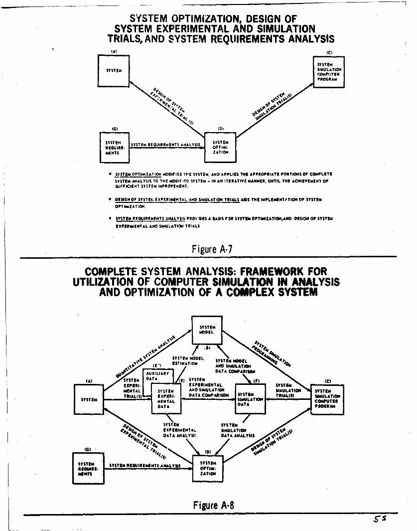
SYSTEM OPTIMIZATION, DESIGN OFSYSTEM EXPERIMENTAL AND SIMULATION
TRIALS, AND SYSTEM REQUIREMENTS ANALYSIS(Al IC)
SYSTEMSYSTEM SIMULATION
PROGRAM
SJFCETSYSTEM ISYOSTENT
I DEQU I GNO SYST - EM R E XPI ERMENT AL AN D Y SI MU ATO N T RI ALMI S T E M L M N F I P S S E
t OPIIMZATTIO.
*SYSTEMREIRENT ANALYSIS TO~'E AH EAI MODR1! SYSTEM - IPTIIERTIEZANE.UTILNAN T1E SIEMNI Of YSE
41DSGO YTAEXPERIMENTAL AN D SIMULATION TRIALS AISTEMP mMlTHOFYTM
Figure A-7
COMPLETE SYSTEM ANALYSIS: FRAMEWORK FORUTILIZATION OF COMNPUTER SINWULATIOPI 114 ANALYSIS
AND OPTIMIZATION OF A COMPLEX SYSTEM
FigurEMAMODEL
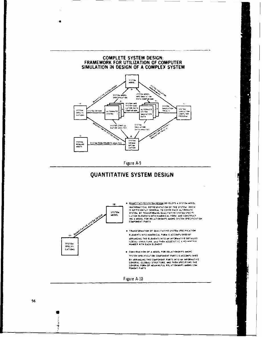
COMPLETE SYSTEM DESIGN:FRAMEWORK FOR UTILIZATION OF COMPUTER
SIMULATION 'N DESIGN OF A COMPLEX SYSTEM
QUANTTATIE SYSEMMODEL~
MATHMTIA RER NTTO OL TA' ,Y M WOICDATAFICILN AIYW.NEA TOC EREC ALRAE
SIT % YSTEM BYTANFRMN QAITTV SYSTEM SECI~ MODEL LCATNIOH EET INTO NUMEICL "OR AN D CONST RUCSHG A MOE FOSTE DESIGNHHPP AMONGM SYSTEMW SPECFICTISr CCO SPSTE M PAMPUTS
S ASTEM 0 TRNSOMUATIONOP ULTTV4YSE PCFCTO
CAT DONS
SYSTEM SCCFCTO COPOEN PA.T IS ACCOMLISE
RB!AAL Y ARRANSING TU CLPNN PAT INT ION INOMTV
GENERTAL GLOALY S TR CUE ADTENSEIYN H
aENERAL FOR OP MEANNGFU RELTINSIP AMONG ANLO..iE aS.ENF z ENT FI0 T
Figure A-9
56NIAIESYTMDSG
0 UNIAIESSE EU,0 EEO$ASSE OE
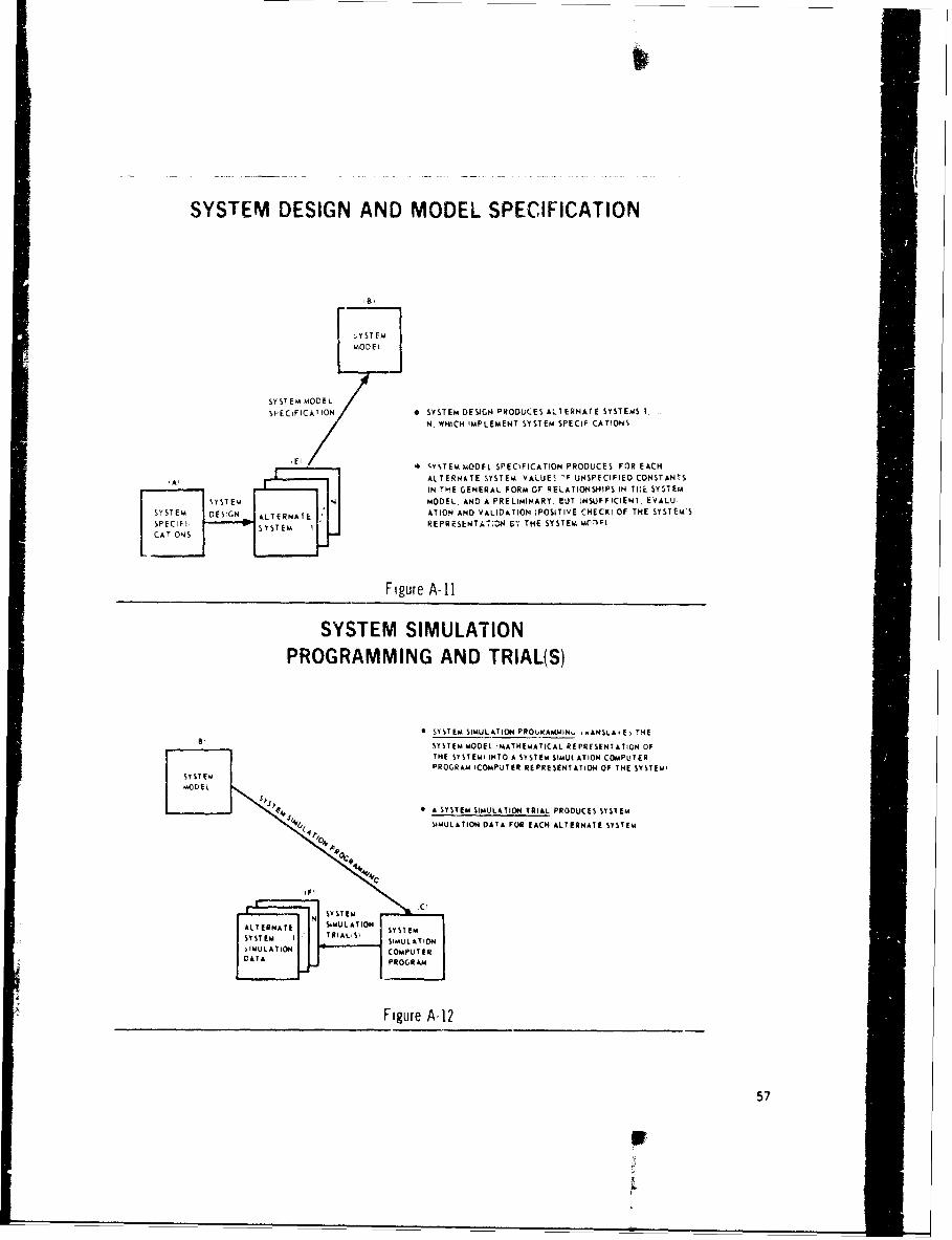
LII
(SYSTEM DESIGN AND MODEL SPECIFICATION
18,
,YST EMMODEL
SYSTEM MODELSPECIFICATION 0 SYSTEM DESIGN PRODUCES ALTERNATE SYSTEMS I.
N, WHICH IMPLEMENT SYSTEM SPECIFICATIONS.
0 SYSTEM MODFL SPECIFICATION PRODUCES FOR EACH
-A, mALTERNATE SYSTEM VALUE! 'F UNSPECIFIED CONSTANTS
IN THE GENERAL FORM or RELATIONSHIPS IN THi SYSTEM
ý~ H MODEL. AND A PRELIMINARY, BUT INSUFFICIENTr EVALU-
SYSTEM DESIGN I nALTERNATE ATION AND VALIDATION IPOSITIVE CHECK) OF THE SYSTEM'S
SPECiFI. • v ISYSTEM I REPRESENTAT;: N F. THE SYSTEM Mr,71 :!CATIONS
Figure A-11
SYSTEM SIMULATIONPROGRAMMING AND TRIAL(S)
9 SYSTEm SIMULATION PROUNAMMINM. .. ANSLA, Ei THE
, SYSTEM MODEL iMATHEMATICAL REPRESENTATION OF
THE SYSTEMI INTO A SYSTEM SIMU( ATION COMPUTERPROGRAM ICOMPUTER REPRESENTATION OF THE SYSTEMI
SY STE M
MODEL
4 A SYSTEM SIMULATION TRIAL PRODUCES SYSTEM
"S J41, SIMULATION DATA FOR EACH ALTERNATE SYSTEM
Ie A*L2N SS57
N SYSTEMALTERN llATEO , SIMULATION SSE
DATAPROGRAM
Figure A-12
57
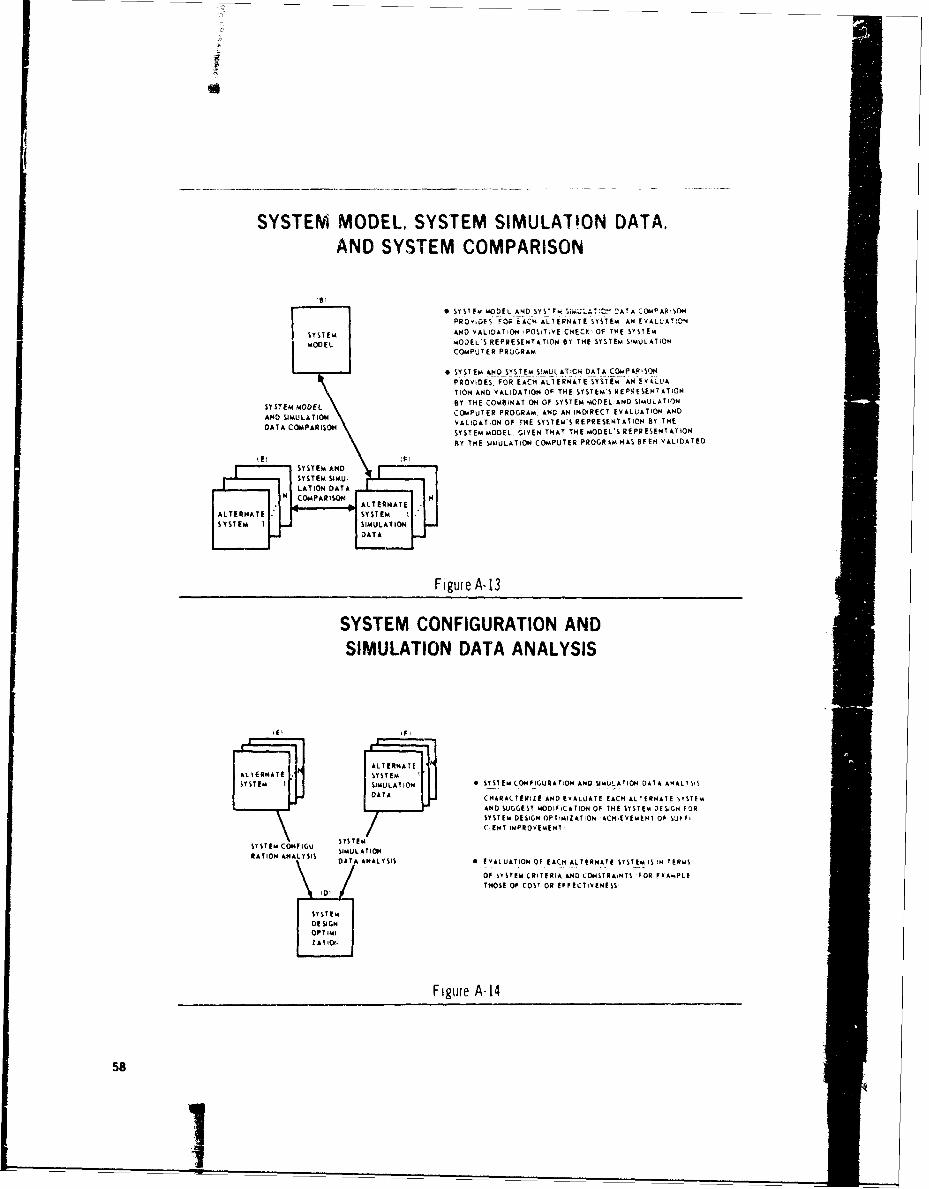
SYSTEM MODEL, SYSTEM SIMULATION DATA.AND SYSTEM COMPARISON
!B
"*SYSTFM MODELANDSYSTY L!. 7!UT' :!AT A COMPARSO.'I
PROv DFS FOR tACH ALTERNATE SYSTEM AN EVALUATION
SYSTEM AND VALIDATION POS ITIVE CHECIK OF THE SYSTEM
MODEL MODEL'S REPRESENTATION BY THE SYSTEM SIMULATION
COMPUTER PROGRAM
"* SYSTEM AND SYSTEM SIMULATICON DATA CO•PAR SONZPROVIDES. FOR EACH ALTERNATE SYSTEM AN EVALUA
TION AND VALIDATION OF THE SYSTEM'S REPRESENTATION
SYSTEM MODE BY THE COMBINATION OF SYSTEM MODEL AND SIMULATION
AND SIMULATION COMPUTER PROGRAM. AHN AN INDIRECT EVALUATION AND
DATA COMPARISON VALIDATION OF THE SYSTEM'S REPRESENTATION BY THE
SYSTEM MODEL GIVEN THAT THE MODEL'S REPRESENTATION
BY THE SIMULATION COMPUTER PROGRAM HAIS FEN VALIDATED
SYYSTEM AND
Figure A-13
SYSTEM CONFIGURATION ANDSIMULATION DATA ANALYSIS[~r~1 1 ]ALTERNATE
SYSSTEM ISESIMULATION * SYSTEM CONFFGURATTON AND SIULATION DATA ANALYS
I I [ J AA CHARACTER ZR AND EVALUATE EACH ALTERNATE VYSTRMSMANU SUGGEST MODFOCATION OF THE SYSTEM DESIGN FOR
SYSTEM DESIGN OPT NIZATION 'ACHIEVEMENT OF SNFFI
TSYSTEM C TMPROVEMENT
SYSTEM CONFIGU SIMULATION
ANDU ATOSTMDF.AIN FIM YTE EIG OSYSTEM DEIGNALYSISN ACIVEtT F$UF
RATION ANALYSIS DATA ANALYSIS 0 EVALUATION OF EACH ALTERNATE SYSTEM IS IN TERMS
OF IYSTEM CRITERIA, AND CONSTRAINTS 'FOR FXAMPLE
THOSE OF COST OR EFFECTIVENESS-
ISYSTEM
IDESIGN I
Figure A-14
58
I
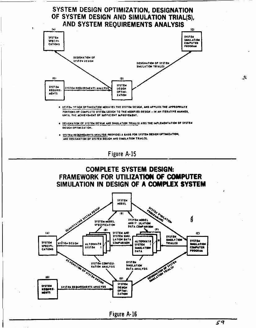
SYSTEM DESIGN OPTIMIZATION, DESIGNATIONOF SYSTrEM DESIGN AND SIMULATION TRIAL(S),
AND SYSTEM REQUIREMENTS ANALYSIS (CSYSTEMSYSTEMsvsr ~SIMULATION
SPE1C IF I. COMOUTERCATIONS PROGRAM
DESIGNATION OFSYSTEM DESIGN
SIMULATION TRIAL(S)
POTM SYTMRtIONS CMPENTE ANAYSTE EIG TOHEMOFD DESIGN -I l TRTV ANUNTIL THE. ACIVMNOPUFCE T IMPRVMET
EWS IG OPTIIZAION
* SYSTEM G EO PTIR MIZNTIOANA S PROVIDES AT ASHE O SYSTEM DESIGN. N A OL THAPTIMIZ IATION
"A4 DESIGNATION Of SYSTEM D ESIG N AND SIM U JLATION TRIAL ( IS).EIPEMNAIN FSSE
Figure A-15
COMPLETE SYSTEM DESIGN:FRAMEWORK FOR UTILIZATIOCMN OW %CdOMPUTER
SIMULATION IN DESIGN OF A COMPLEX SYSTEM,SYSTEM
(9)9