Embed Size (px)
Citation preview
UCGE Reports Number 20383
Department of Geomatics Engineering
Ionospheric Imaging for Canadian Polar Regions
(URL: http://www.geomatics.ucalgary.ca/graduatetheses)
by
Ossama Jamil Saleh Al-Fanek
August, 2013
UNIVERSITY OF CALGARY
Ionospheric Imaging for Canadian Polar Regions
by
Ossama Jamil Saleh Al-Fanek
A THESIS
SUBMITTED TO THE FACULTY OF GRADUATE STUDIES
IN PARTIAL FULFILMENT OF THE REQUIREMENTS FOR THE
DEGREE OF DOCTOR OF PHILOSOPHY
DEPARTMENT OF GEOMATICS ENGINEERING
CALGARY, ALBERTA
August, 2013
© Ossama Jamil Saleh Al-Fanek 2013

ii
Abstract
Global Navigation Satellite Systems (GNSS) can be exploited as a cost-effective tool to remotely
sense the Earth’s ionosphere and investigate its characteristics. This is due to the global coverage
and dual frequency data availability offered through worldwide networks of GNSS stations.
Since the ionosphere is a dispersive medium, the dual frequency data can be utilized to derive
highly accurate Slant Total Electron Content (STEC) measurements. STEC is defined as the
integration of the free electron distribution in a 1-m2 column along the signal path from the
satellite to the receiver. Although STEC provides a valuable source of information about the
ionosphere, these measurements do not contain any spatial information about the electron density
distribution along the line-of-sight. Therefore, a tomographic technique is required to retrieve
such three-dimensional information.
Measurement of the polar ionosphere is challenging due to its variable nature and typically
limited availability of ground (or space) based infrastructure for remote sensing. An opportunity
exists to exploit GNSS observations for ionospheric imaging in this region. Ten GNSS reference
stations of the Canadian High Arctic Ionospheric Network (CHAIN), augmented with six
International GNSS Service (IGS) polar reference stations, provides sufficient observations for
GNSS-based tomographic estimation of key polar ionospheric parameters. Polar implementation
of tomographic imaging for such a sparse network presents major challenges, however, and
requires novel methods.
In this thesis, a novel Computerized Ionospheric Tomographic (CIT) reconstruction technique is
developed to estimate electron density profiles over the Canadian polar region. This technique
divides the ionosphere into voxels where the electron density is assumed to be homogeneous

iii
within a voxel. A functional based model is used to represent the electron density in space. The
functional based model uses Empirical Orthogonal Functions (EOF) and Spherical Cap
Harmonics (SCH) to describe the vertical and horizontal distribution of the electron density,
respectively. Simulated and real data are used to demonstrate the feasibility and performance of
the technique under different ionospheric conditions. The main aspects of the reconstruction
results over the Canadian polar cap are highlighted and discussed and a clear understanding of
the quality and limitations of the technique is achieved.

iv
Preface
The Computerized Ionospheric Technique (CIT) described in Chapter 4 has been previously
published in a conference paper:
Al-Fanek, O. and Skone, S. (2011), “Ionospheric Imaging Using GNSS: A New
Approach for Canadian Polar Regions”, Presented at the Proceedings of ION GNSS
2011, September 2023, Portland, OR, pp. 643-653.
The author’s research work from the paper has been extended in this thesis.

v
Acknowledgements
First and Foremost, I wish to express my deepest gratitude to my advisor Dr. Susan Skone for the
continuous support, for her patience, time and immense knowledge. I would never have been
able to finish my dissertation without your excellent guidance and technical advice.
I would like to thank the UCAR/COSMIC program and the Canadian High Arctic Ionospheric
Network (CHAIN) for providing the on-line access to COSMIC Radio Occultation (RO) and
GPS data, respectively. Infrastructure funding for CHAIN is provided by the Canada Foundation
for Innovation and the New Brunswick Innovation Foundation. CHAIN operation is conducted
in collaboration with the Canadian Space Agency. I would also like to acknowledge the use of
the IRI model which was kindly made available online.
Special thanks are extended to my friends, Oday Haddad, Mohannad Al-Durgham, Eunju Kwak,
Qais Marji, Samer Chomery, Dima Oweis, Violin Narooz, Philip Nour, and Victor Halim for all
your support. You are the best! A special appreciation is reserved to my friend Kaleel Al-
Durgham. Your encouraging words and support will never be forgotten.
My sincere thanks and gratitude goes to my parents, brothers and sister for the love and support
they have provided me over the years.
Finally, I would like to thank my wife, Ghena Azar. You have always had faith in me and stood
by me through the good and bad times. You have been my inspiration and motivation for
success. This thesis is dedicated to you.

vi
Dedication
To my wife
vii
Table of Contents
Abstract ............................................................................................................................... ii
Preface................................................................................................................................ iv
Acknowledgements ..............................................................................................................v
Dedication .......................................................................................................................... vi
Table of Contents .............................................................................................................. vii
List of Tables .......................................................................................................................x
List of Figures .................................................................................................................... xi
List of Abbreviations .........................................................................................................xv
CHAPTER ONE: INTRODUCTION ..................................................................................1
1.1 Background and Motivation ......................................................................................1
1.2 Research Objectives and Contributions .....................................................................5
1.3 Thesis Outline ............................................................................................................6
CHAPTER TWO: THE GLOBAL POSITIONING SYSTEM (GPS) ................................9
2.1 Overview ....................................................................................................................9
2.1.1 The Space Segment ...........................................................................................9
2.1.2 The Control Segment .......................................................................................10
2.1.3 The User Segment ...........................................................................................11
2.2 GPS Signal Structure ...............................................................................................11
2.3 GPS Observables .....................................................................................................13
2.4 GPS Error Sources ...................................................................................................14
2.4.1 Orbital Errors ...................................................................................................16
2.4.2 Satellite Clock Errors ......................................................................................16
2.4.3 Receiver Clock Errors .....................................................................................18
2.4.4 Receiver Noise .................................................................................................18
2.4.5 Multipath .........................................................................................................19
2.4.6 Tropospheric Errors .........................................................................................19
2.4.7 Ionospheric Errors ...........................................................................................20
2.5 Satellite Geometry ...................................................................................................20
2.6 Differential GPS ......................................................................................................22
CHAPTER THREE: THE IONOSPHERE ........................................................................25
3.1 Structure of the Ionosphere ......................................................................................25
3.2 Ionospheric Characteristics ......................................................................................27
3.2.1 Diurnal Variation .............................................................................................27
3.2.2 Latitudinal Variation .......................................................................................27
3.2.3 Seasonal Variation ...........................................................................................28
3.2.4 Solar Cycle Variation ......................................................................................28
3.3 Ionospheric Models ..................................................................................................30
3.3.1 Chapman Profile ..............................................................................................30
3.3.2 International Reference Ionosphere (IRI) ........................................................31
3.3.3 Parameterized Ionospheric Model (PIM) ........................................................31
3.4 Ionospheric Effects on GPS Signals ........................................................................32
3.5 TEC Variation ..........................................................................................................36
viii
CHAPTER FOUR: IONOSPHERIC TOMOGRAPHY ....................................................39
4.1 Introduction ..............................................................................................................39
4.2 Tomography Problem ..............................................................................................39
4.3 Data Geometry Effect ..............................................................................................41
4.4 Overview of Ionospheric Tomography Development .............................................43
4.5 Extracting Ionospheric Information from GPS Observables ...................................47
4.5.1 STEC Observation ...........................................................................................47
4.5.2 STEC Smoothing .............................................................................................49
4.5.3 Cycle Slip Detection ........................................................................................52
4.6 Model Development ................................................................................................54
4.6.1 Voxel-Based Model .........................................................................................54
4.6.1.1 Design of 3-D Voxel-Based Model .......................................................58
4.6.2 Spherical Cap Harmonics (SCH) .....................................................................61
4.6.2.1 Coordinate Transformation ....................................................................63
4.6.2.2 Computation of the Associated Legendre Function cosPm
n k .............65
4.6.3 Empirical Orthogonal Functions (EOF) ..........................................................67
4.7 Weighted Least Squares ...........................................................................................71
4.8 Generalized Tikhonov Regularization .....................................................................72
4.8.1 Regularization Parameter Selection ................................................................74
4.9 Advantages of Ionospheric Tomography .................................................................75
4.10 Applications of Ionospheric Tomography .............................................................75
CHAPTER FIVE: IONOSPHERIC TOMOGRAPHY MODELLING – SIMULATION 77
5.1 Introduction ..............................................................................................................77
5.2 Tomographic Modelling of Canadian Polar Region ................................................77
5.3 Simulated Data Description .....................................................................................78
5.4 Data Analysis Strategy and Results Validation .......................................................82
5.5 Numerical Simulation ..............................................................................................84
5.5.1 Simulation of Nominal Ionospheric Conditions ..............................................90
5.5.2 Simulation of Storm Ionospheric Conditions ..................................................95
5.6 Determination of SCH and Number of EOF............................................................97
5.7 Model Evaluation .....................................................................................................98
5.7.1 Nominal Ionospheric Conditions .....................................................................98
5.7.2 Storm Conditions ...........................................................................................111
5.8 Chapter Summary ..................................................................................................114
CHAPTER SIX: IONOSPHERIC TOMOGRAPHY MODELLING – REAL DATA ...116
6.1 Introduction ............................................................................................................116
6.2 Results Validation ..................................................................................................117
6.2.1 Radio Occultation ..........................................................................................117
6.2.2 Stability of Receiver Inter-Frequency Biases (IFB) ......................................118
6.3 Data Description and Analysis Strategy ................................................................121
6.4 Constraining the Ionospheric Tomography Problem .............................................122
6.5 Data Analysis and Results .....................................................................................125
6.5.1 Nominal Ionospheric Conditions ...................................................................126
6.5.1.1 Inter-Frequency Bias Stability .............................................................131
ix
6.5.1.2 Electron Density Profile Comparisons ................................................134
6.5.2 Disturbed Ionospheric Conditions .................................................................141
6.6 Chapter Summary ..................................................................................................152
CHAPTER SEVEN: CONCLUSIONS AND RECOMMENDATIONS ........................153
7.1 Conclusions ............................................................................................................153
7.2 Recommendations ..................................................................................................155
REFERENCES ................................................................................................................157

x
List of Tables
Table 2.1: Components of the GPS satellite signal (after Hofmann-Wellenhof et al., 2007) ...... 12
Table 4.1: Non-integer degrees m
kn for half-angle o = 24 .......................................................... 66
Table 5.1: Station coordinates of the Canadian polar region network .......................................... 80
Table 5.2: Simulation settings....................................................................................................... 96
Table 5.3: Assessment of the model using Kmax = 3 and Q = 3 .................................................. 103
Table 5.4: Statistics on the vertical TEC error on 01 January 2000. .......................................... 111
Table 5.5: Error statistics using different Kmax and Q................................................................. 112
Table 6.1: Model settings ............................................................................................................ 122
Table 6.2: Root mean square of the residuals in TECU (Kmax =3 and Q = 3) ............................ 131
Table 6.3: Estimated inter-frequency receiver biases (Kmax =3 and Q = 3) ................................ 133
Table 6.4: Summary of the statistics of the difference between the electron density profiles
derived by radio occultation vs. CIT (Kmax =3 and Q = 3) ................................................. 137
Table 6.5: Statistics of the difference between the electron density profiles derived by radio
occultation vs. CIT for 16 January 2010 (Kmax =3 and Q = 3) ........................................... 138
Table 6.6: Statistics of the difference between the electron density profiles derived by radio
occultation vs. CIT for 01 May 2010 (Kmax =3 and Q = 3) ................................................ 139
Table 6.7: Statistics of the difference between the electron density profiles derived by radio
occultation vs. CIT for 11 December 2010 (Kmax =3 and Q = 3) ....................................... 140
Table 6.8: Root mean square of the residuals in TECU (Kmax =3 and Q = 3) ............................ 145
Table 6.9: Estimated inter-frequency receiver biases for 10 September 2011 (Kmax =3 and Q
= 3) ...................................................................................................................................... 146
Table 6.10: Statistics of the difference between the electron density profiles derived by radio
occultation vs. CIT for 10 September 2011 (Kmax =3 and Q = 3) ....................................... 147
xi
List of Figures
Figure 2.1: GPS orbital configuration ........................................................................................... 10
Figure 2.2: GPS Error Sources...................................................................................................... 16
Figure 2.3: Good and poor satellite geometry .............................................................................. 21
Figure 2.4: Differential GPS ......................................................................................................... 23
Figure 2.5: Wide Area Differential GPS System .......................................................................... 24
Figure 3.1: Ionospheric layers. at night, F1 and F2 layers combine into F layer and D layer
disappears .............................................................................................................................. 26
Figure 3.2: Typical day/night electron density profiles. ............................................................... 28
Figure 3.3: Monthly and monthly smoothed sunspot numbers since 1954.
(http://sidc.oma.be/html/wolfmms.html, April 2013) ........................................................... 29
Figure 3.4: Different electron density profiles based on different sun zenith angles using
Chapman profile. (scale height = 75 km, reference height = 300 km, and = 1012
el/m3). .................................................................................................................................... 30
Figure 3.5: IRI-2007 and PIM profiles (Calgary, Canada 51.05° N, 114.07° W) . ...................... 32
Figure 3.6: Ionospheric range delay using Equation (3.12) .......................................................... 35
Figure 3.7: Variation in TEC with local time, season and sunspot number for middle latitudes . 36
Figure 3.8: Global Ionospheric Map (GIM) (data courtesy of CODE) ........................................ 37
Figure 3.9: An example of SED over Canadian latitudes during a geomagnetic storm event
on 30 October 2003 between 21:02 and 21:32 UT ............................................................... 38
Figure 4.1: A simple tomography example................................................................................... 40
Figure 4.2: Effect of data geometry on tomography ..................................................................... 42
Figure 4.3: Comparison of code-derived (STECP ), phase-derived (STEC ) and smoothed STEC (STECsmoothed ) calculated along the slant signal path of GPS satellite 7 observed
from ALGO on January 1, 2010. .......................................................................................... 51
Figure 4.4: Geometry involved in ionospheric tomography ......................................................... 55
Figure 4.5: Schematic of voxel-modeled electron distribution over a GPS network ................... 56
Figure 4.6: Voxel sides definition ................................................................................................. 60
xii
Figure 4.7: Observation rejection criteria ..................................................................................... 61
Figure 4.8: The pole of spherical cap coordinate system (after Liu et al., 2009). ........................ 64
Figure 4.9: Coordinate transformation between geographic coordinate system and spherical
cap coordinate system (after Liu et al., 2009). ...................................................................... 65
Figure 4.10: Associated Legendre functions for a spherical cap of half-angle o = 24,
for k = 5, m = 0, 1, … 5 .......................................................................................................... 67
Figure 4.11: First three EOFs derived from IRI-2007 model ....................................................... 69
Figure 4.12: The L-curve .............................................................................................................. 74
Figure 5.1: The geographic distribution of the IGS and CHAIN stations based on Google
EarthTM
. ................................................................................................................................. 79
Figure 5.2: Solar Cycle Sunspot Number (http://www.swpc.noaa.gov/SolarCycle/, July 2013) . 82
Figure 5.3: Spherical cap boundary (red) and voxel footprints (green) ........................................ 87
Figure 5.4: Computation of vertical TEC ..................................................................................... 88
Figure 5.5: Flow chart summarizing the simulation and validation procedure ............................ 89
Figure 5.6: Simulated STEC along PRN 3 line-of-sight for Churchill site in solar maximum
(top) and solar minimum (bottom) ........................................................................................ 91
Figure 5.7: Comparison of reference diurnal IRI-TEC variation for solar maximum (red),
moderate (blue) and solar minimum (green)......................................................................... 92
Figure 5.8: Comparison of reference diurnal maximum IRI-TEC variation for solar maximum
(red), moderate (blue) and solar minimum (green) in the Canadian sector .......................... 93
Figure 5.9: Simulated Vertical TEC for 01-January of years 2000 (top), 2004 (middle) and
2009 (bottom) for 10:00 UT(left) and 21:00 UT(right) ........................................................ 94
Figure 5.10: Simulated electron density profile (left) and vertical TEC map (right) of a storm
enhanced density ................................................................................................................... 96
Figure 5.11: Average maximum peak value error for 01-January of years 2000 (top), 2004 (middle) and 2009 (bottom) for UT 10:00 (left) and UT 21:00 (right) ............ 100
Figure 5.12: Mean absolute error (MAE) in TEC for 01-January of years 2000 (Top), 2004
(Middle) and 2009 (Bottom) for UT 10:00 (Left) and UT 21:00 (Right) ........................... 101
Figure 5.13: Reconstruction error (Re) for 01-January of years 2000 (top), 2004 (middle) and
2009 (bottom) for UT 10:00 (left) and UT 21:00 (right) .................................................... 102

xiii
Figure 5.14: Estimated vertical TEC maps using simulated IRI STEC (left) and the difference
between the estimated and simulated TEC maps (right) for 01 January 2000 (top), 2004
(middle) and 2009 (bottom) for UT 21:00 (Kmax =3 and Q = 3) ......................................... 105
Figure 5.15: Simulated (left) and estimated (right) electron density distribution IRI along
270 E longitude for 01 January 2000 (top), 2004 (middle) and 2009 (bottom) for UT 21:00 (Kmax =3 and Q = 3) .................................................................................................. 106
Figure 5.16 Histogram of the residuals for 01 January 2000 (top), 2004 (middle) and 2009
(bottom) for UT 21:00 (Kmax =3 and Q = 3) ....................................................................... 108
Figure 5.17:Comparison between simulated (top), estimated (middle) vertical TEC maps and
the error in the estimation (bottom). Results are shown for 01 January 2000 for UT
00:00 (left) and UT 06:00 (right) using Kmax =3 and Q = 3. ............................................... 109
Figure 5.18 Comparison between simulated (top), estimated (middle) vertical TEC maps and
the error in the estimation (bottom). Results are shown for 01 January 2000 for UT
12:00 (left) and UT 18:00 (right) using Kmax =3 and Q = 3. ............................................... 110
Figure 5.19: Estimated vertical TEC map (left) and the error in the estimation (right) using
Kmax =3 and Q = 3. .............................................................................................................. 112
Figure 5.20:Refined vertical TEC map (left) and the error in the estimation (right). ................. 113
Figure 5.21: Estimated electron density profile along 266.5 E longitude. Results are shown
for CIT using SCH and EOF (left) and constrained CIT (right) ......................................... 114
Figure 6.1: Illustration of the geometry of the GPS-LEO for ionospheric sounding. ................ 117
Figure 6.2: Illustration of the effect of orientation on geometry ................................................ 123
Figure 6.3: Estimated electron density profile before (left) and after (right) applying
constraint. ............................................................................................................................ 125
Figure 6.4: Planetary Kp indices for 16 January 2010 (top), 01 May 2010 (middle), and 11
December 2010 (bottom)
(http://www.swpc.noaa.gov/ftpmenu/warehouse/2011/2011_plots.html, April 2013) ...... 127
Figure 6.5: Estimated vertical TEC maps for 16 January 2010 (Kmax =3 and Q = 3) ................. 128
Figure 6.6: Estimated vertical TEC maps for 01 May 2010 (Kmax =3 and Q = 3) ...................... 129
Figure 6.7: Estimated vertical TEC maps for 11 December 2010 (Kmax =3 and Q = 3) ............. 130
Figure 6.8: Relative receiver inter-frequency biases for 16 January 2010 (top), 01 May 2010
(middle), and 11 December 2010 (bottom) (Kmax =3 and Q = 3) ....................................... 132
xiv
Figure 6.9: Radio occultation (RO) vs. tomography (TOMO) electron density profiles for 16
January 2010 ....................................................................................................................... 135
Figure 6.10: Radio occultation (RO) vs. tomography (TOMO) electron density profiles for 01
May 2010 ............................................................................................................................ 136
Figure 6.11: Radio occultation (RO) vs. tomography (TOMO) electron density profiles for 11
December 2010 ................................................................................................................... 137
Figure 6.12: Planetary Kp indices for 10 September 2011
(http://www.swpc.noaa.gov/ftpmenu/warehouse/2011/2011_plots.html, April 2013) ...... 142
Figure 6.13: Local K-index for 9-10 September, 2011 (data courtesy of NRCAN) .................. 142
Figure 6.14: Geomagnetic field observations for Canadian magnetic observatories for 10
September, 2011 (http://www.geomag.nrcan.gc.ca; April 2013) ....................................... 143
Figure 6.15: Estimated vertical TEC maps for 10 September 2011 (Kmax =3 and Q = 3) .......... 144
Figure 6.16: Comparison of JPL relative receiver inter-frequency biases for 10 September
2011 (Kmax =3 and Q = 3) ................................................................................................... 146
Figure 6.17: Vertical TEC (top) and Nemax (bottom) over 47.5N and 270 E for September 2011 ..................................................................................................................................... 149
Figure 6.18: Dst index for 09-10 September, 2011 (data courtesy of World Data Center for
Geomagnetism, Kyoto) ....................................................................................................... 150
Figure 6.19: Interplanetary magnetic field (top) and the solar wind velocity, X component
(bottom) for 09 September, 2011. (http://cdaweb.gsfc.nasa.gov; April 2013) ................... 151

xv
List of Abbreviations
Symbol Definition
AFB Air Force Base
ART Algebraic Reconstruction Technique
C/A code Coarse/Acquisition code
CADI Canadian Advanced Digital Ionosondes
CDAAC COSMIC Data Analysis and Archive Center
CHAIN Canadian High Arctic Ionospheric Network
CIT Computerized Ionospheric Tomography
CL code Civilian Long length code
CM code Civilian Moderate code
COSMIC Constellation Observing System for the
Meteorology, Ionosphere and Climate
COSPAR Committee on Space Research
DGPS Differential GPS
DoD Department of Defense
DOP Dilution of Precision
Dst Disturbed Storm Time
EDOP Easting Dilution of Precision
EGNOS European Geostationary Navigation Overlay
Service
EOF Empirical Orthogonal Functions
ESA European Space Agency
EUV Extreme Ultra Violet
FAA Federal Aviation Administration
GNSS Global Navigation Satellite System
GPS Global Positioning System
GSVD Generalized Singular Value Decomposition
GTIM Global Theoretical Ionospheric Model
HDOP Horizontal Dilution of Precision
HF High Frequency
IFB Inter-Frequency Bias
IGS International GNSS Service
IMF Interplanetary Magnetic Field
IRI International Reference Ionosphere
ISIS International Satellites for Ionospheric Studies
JPL Jet Propulsion Laboratory
LADGPS Local-Area Differential GPS
LEO Low-Earth Orbiting
LOS Line-of-Sight
LT Local Time
LUF Lowest Usable Frequency
MAE Mean Absolute Error
xvi
MART Multiplicative Algebraic Reconstruction
Technique
MCS Master Control Station
MUF Maximum Usable Frequency
NDOP Northing Dilution of Precision
NNSS Navy Navigation Satellite System
OCXO Oven Controlled Crystal Oscillator
P-code Precise code
PDOP Position Dilution of Precision
PIM Parameterized Ionospheric Model
ppm Parts per million
PRN Pseudo Random Noise
RMS Root Mean Square
RO Radio Occultation
SA Selective Availability
SCH Spherical Cap Harmonics
SCHA Spherical Cap Harmonic Analysis
SED Storm Enhanced Density
SHA Spherical Harmonics Analysis
SIRT Simultaneous Iterative Reconstruction Technique
SSN Sunspot Number
STEC Slant Total Electron Content
SVD Singular Value Decomposition
TCXO Temperature Compensated Crystal Oscillator
TDIM Time Dependent Ionospheric Model
TDOP Time Dilution of Precision
TEC Total Electron Content
URSI International Union of Radio Science
UT Universal Time
VDOP Vertical Dilution of Precision
WAAS Wide Area Augmentation System
WADGPS Wide-Area Differential GPS
WGS-84 World Geodetic System 1984

1
Chapter One: Introduction
This chapter presents the research background, research motivation and objectives.
1.1 Background and Motivation
The ionosphere is the ionized part of the upper region of the atmosphere extending from 60 km
to 1500 km above the Earth’s surface, where free electrons are produced during the interaction of
Extreme Ultra Violet (EUV) and X-ray radiation with the upper neutral atmosphere. Knowledge
of the ionospheric electron density distribution is important for scientific studies and practical
applications. From the applications perspective, the electron density is the most important
ionospheric parameter due to its effect on radio frequency electromagnetic wave propagation.
For scientific studies, measuring ionospheric parameters, especially the electron density, helps to
understand the solar-terrestrial interaction and provide more information about the spatial
variations in ionospheric plasma and its evolution in time (Bust and Mitchell, 2008).
Global Navigation Satellite Systems (GNSS), such as the Global Positioning System (GPS), are
regarded as important cost effective tools to remotely sense the Earth’s ionosphere and
investigate its characteristics. This is due to the global system coverage and multiple frequency
data available via a world-wide network of GNSS stations. Since the ionosphere is a dispersive
medium, this multiple frequency data can be used to derive the integrated measurements of
electron density, known as Total Electron Content (TEC), along the line-of sight between a given
satellite and receiver. By collecting TEC measurements from network of dual frequency GNSS
receivers, useful information about the ionosphere can be derived and ionospheric models can be
developed.
Ionospheric models usually represent average conditions and are mostly based on the bottom
side of the ionosphere (i.e. the region below the maximum electron density which generally
2
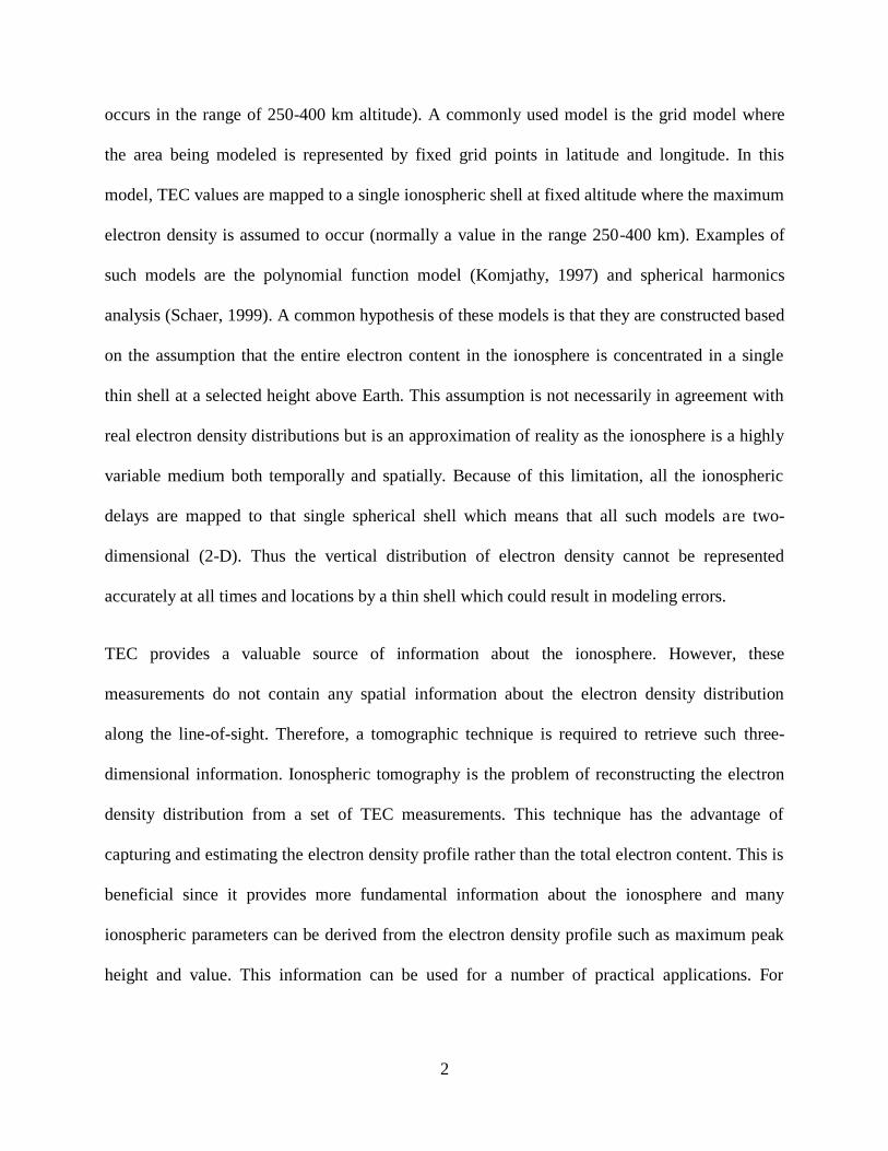
occurs in the range of 250-400 km altitude). A commonly used model is the grid model where
the area being modeled is represented by fixed grid points in latitude and longitude. In this
model, TEC values are mapped to a single ionospheric shell at fixed altitude where the maximum
electron density is assumed to occur (normally a value in the range 250-400 km). Examples of
such models are the polynomial function model (Komjathy, 1997) and spherical harmonics
analysis (Schaer, 1999). A common hypothesis of these models is that they are constructed based
on the assumption that the entire electron content in the ionosphere is concentrated in a single
thin shell at a selected height above Earth. This assumption is not necessarily in agreement with
real electron density distributions but is an approximation of reality as the ionosphere is a highly
variable medium both temporally and spatially. Because of this limitation, all the ionospheric
delays are mapped to that single spherical shell which means that all such models are two-
dimensional (2-D). Thus the vertical distribution of electron density cannot be represented
accurately at all times and locations by a thin shell which could result in modeling errors.
TEC provides a valuable source of information about the ionosphere. However, these
measurements do not contain any spatial information about the electron density distribution
along the line-of-sight. Therefore, a tomographic technique is required to retrieve such three-
dimensional information. Ionospheric tomography is the problem of reconstructing the electron
density distribution from a set of TEC measurements. This technique has the advantage of
capturing and estimating the electron density profile rather than the total electron content. This is
beneficial since it provides more fundamental information about the ionosphere and many
ionospheric parameters can be derived from the electron density profile such as maximum peak
height and value. This information can be used for a number of practical applications. For
3
example the peak height of electron density is used in monitoring and predicting HF
communication capabilities for aircraft polar routes.
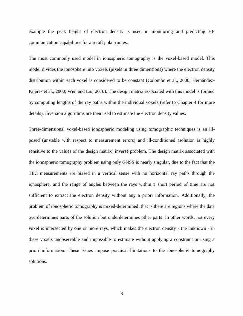
The most commonly used model in ionospheric tomography is the voxel-based model. This
model divides the ionosphere into voxels (pixels in three dimensions) where the electron density
distribution within each voxel is considered to be constant (Colombo et al., 2000; Hernández-
Pajares et al., 2000; Wen and Liu, 2010). The design matrix associated with this model is formed
by computing lengths of the ray paths within the individual voxels (refer to Chapter 4 for more
details). Inversion algorithms are then used to estimate the electron density values.
Three-dimensional voxel-based ionospheric modeling using tomographic techniques is an ill-
posed (unstable with respect to measurement errors) and ill-conditioned (solution is highly
sensitive to the values of the design matrix) inverse problem. The design matrix associated with
the ionospheric tomography problem using only GNSS is nearly singular, due to the fact that the
TEC measurements are biased in a vertical sense with no horizontal ray paths through the
ionosphere, and the range of angles between the rays within a short period of time are not
sufficient to extract the electron density without any a priori information. Additionally, the
problem of ionospheric tomography is mixed-determined: that is there are regions where the data
overdetermines parts of the solution but underdetermines other parts. In other words, not every
voxel is intersected by one or more rays, which makes the electron density - the unknown - in
these voxels unobservable and impossible to estimate without applying a constraint or using a
priori information. These issues impose practical limitations to the ionospheric tomography
solutions.
4
To overcome these limitations, many authors have used a functional representation of the
electron density and transformed the problem to estimate the coefficients of orthogonal basis
functions that describe the electron density distribution. Many functional representations of the
electron density have been used by different authors. However, most of them share the utilization
of Empirical Orthogonal Functions (EOF) to constrain the model vertically. Erturk et al. (2009)
represented the electron density distribution globally as a summation of EOF, where the
International Reference Ionospheric model IRI was used to derive EOFs. Mitchell and Spencer
(2003) used the application of Spherical Harmonic Analysis (SHA) with Empirical Orthogonal
Functions (EOF) to represent the data globally, using the solution to map the electron density
over a restricted region. Spherical Harmonics Analysis (SHA) is well-suited for global
representation but it is very demanding for high resolution models. To represent a field such as
the electron density profile with a short wavelength, a high order of spherical harmonics is
required. As the order and degree of the spherical harmonic expansion increases, the number of
coefficients becomes too large. This imposes large memory requirements and leads to higher
numerical computational cost. Also, higher order and degree generate numerical instabilities in
estimating the coefficients. This makes the model unsuitable for modelling the ionosphere over a
limited sector using a network of GNSS stations.
One region that has attracted a lot of attention in the past decade is the polar cap due to its
importance and effect on radio propagation and communication especially during solar storms
which might cause loss of communication and damage to electrical transmission equipment. The
polar cap region has lacked spatial resolution of TEC measurements due to the orbit limitations
of spaced-based measurements and sparse networks providing such measurements. To overcome
these limitations, the Canadian High Arctic Ionospheric Network (CHAIN) was designed to

5
develop a better understanding of the effect of solar-terrestrial activity on the Earth's
environment. To make use of such a network and provide scientists with other cost effective
sources of information to advance understanding of the ionosphere, a three-dimensional
ionospheric tomographic model for a wide area GNSS network in the Canadian polar region is
required.
1.2 Research Objectives and Contributions
The principle objective of this doctoral thesis is to develop an optimal tomographic model for
determining ionospheric electron density distribution based on observations from a ground-based
regional network of GPS stations in the Canadian polar region. The principle objective can be
achieved by fulfilling the following sub-objectives:
Implement a voxel-based ionospheric tomographic model.
Develop a tool based on existing empirical ionospheric models, such as IRI-2007, to
simulate the electron density distribution.
Obtain a three-dimensional functional representation of the electron density distribution
over a limited sector which reduces the number of unknowns to be estimated, hence
reducing the computational load and memory requirement.
Regularize the underdetermined ill-conditioned ionospheric tomography problem.
Determine the most appropriate settings (Kmax and Q values) of the three-dimensional
functional representation of electron density distribution for the Canadian polar region.
The research contributions of this thesis include:
6
1) A novel Computerized Ionospheric Tomographic (CIT) technique using a voxel-based
model to retrieve a three-dimensional description of the ionospheric electron density
distribution.
2) An implementation of the proposed ionospheric tomographic technique in a MATLAB
software package.
3) An assessment and validation of the performance of the developed tomographic
technique using simulated and real GPS data under various ionospheric conditions.
Limitations and potential of the technique are determined and quantified.
4) An introduction of a reference (pseudo TEC measurement) to estimate the receiver and
satellite Inter-Frequency Biases (IFB)
5) A proposed approach (constraint) to overcome the limitation of bad geometry and
undetected blunders of GPS real data.
1.3 Thesis Outline
This thesis consists of seven chapters:
Chapter 1 states the research background and objectives.
Chapter 2 introduces the fundamental concept of GPS, GPS observables, and error
sources affecting GPS observables.
Chapter 3 contains a review of the ionosphere characteristics and its effect on GPS
signals.
Chapter 4 describes the problem of ionospheric tomography and presents the
development of a novel Computerized Ionospheric Tomographic (CIT) reconstruction
technique for a voxel-based three-dimensional (3-D) tomographic model based on
Empirical Orthogonal Functions (EOF) and Spherical Cap Harmonics (SCH). This

7
chapter also focuses on the extraction of the ionospheric delay observable (STEC) used to
obtain a tomographic description of the electron density distribution using ground-based
GPS data. Tikhonov regularization is also introduced to handle ill-posed problems such
as ionospheric tomography.
Chapter 5 provides an assessment of the implemented tomographic technique using
simulated data. The optimal values of Kmax and Q order of SCH and number of EOF in
the functional representation of the electron density in the proposed model are also
determined. These values are adopted for the processing of real data in Chapter 6.
Simulations of different ionospheric conditions over the Canadian polar region are used
to determine these values and investigate the capability of the technique to recover
different ionospheric parameters such as electron density, TEC, electron density and
maximum peak value. Nominal and storm conditions are simulated and the performance
of the technique under these conditions is analyzed.
Chapter 6 provides a performance analysis of the proposed technique with GPS real data.
A pseudo TEC observation is introduced to estimate the satellite and receiver inter-
frequency biases (IFB). One approach is proposed and used to overcome the limitation of
bad data geometry and undetected errors associated with real data. The optimal values of
Kmax and Q determined in Chapter 5 are adopted in processing the data. Stability of the
IFB and the radio occultation derived electron density profile are used to validate the
results. A study of an ionospheric storm using the implemented CIT is conducted to
demonstrate the applicability of the technique to monitor the ionosphere and provide a
better understanding of the physical processes.

8
Conclusions and recommendation for future work are presented in Chapter 7 based on
development and assessment of the new CIT technique.

9
Chapter Two: The Global Positioning System (GPS)
2.1 Overview
The Global Positioning System (GPS) is a worldwide passive (one-way) satellite-based radio
navigation positioning system that allows a GPS receiver to determine its position based on
trilateration method. The system was approved and developed by the United States Department
of Defense (DoD) starting in 1973 and has been fully operational since 1995. The principal
objective of developing such a system was to enhance the effectiveness of U.S. and allied
military forces by offering accurate estimates of position, velocity and time and, as a by-product,
to serve the civilian community (Parkinson and Spilker, 1996). Due to the GPS near-global
coverage and continuous services independent of the meteorological conditions, this military
navigation system has become an important tool with many applications ranging from mapping
and surveying to international air traffic management and global research. The GPS consists of
three segments: space, control, and user segment. These are described in the next three sub-
sections.
2.1.1 The Space Segment
The space segment utilizes at least 24 satellites (up to 32) with a minimum of four primary
satellites orbiting in each of the six orbital planes that are inclined at 55 degrees with respect to
the equatorial plane. The orbital altitudes are ~20,200 km, with periods of one-half sidereal day
(~11.967h). The orbits are nearly circular, with slight perturbations due to non-sphericity of the
Earth and solar radiation pressure (Hofman-Wellenhof et al., 2001). This orbital configuration is
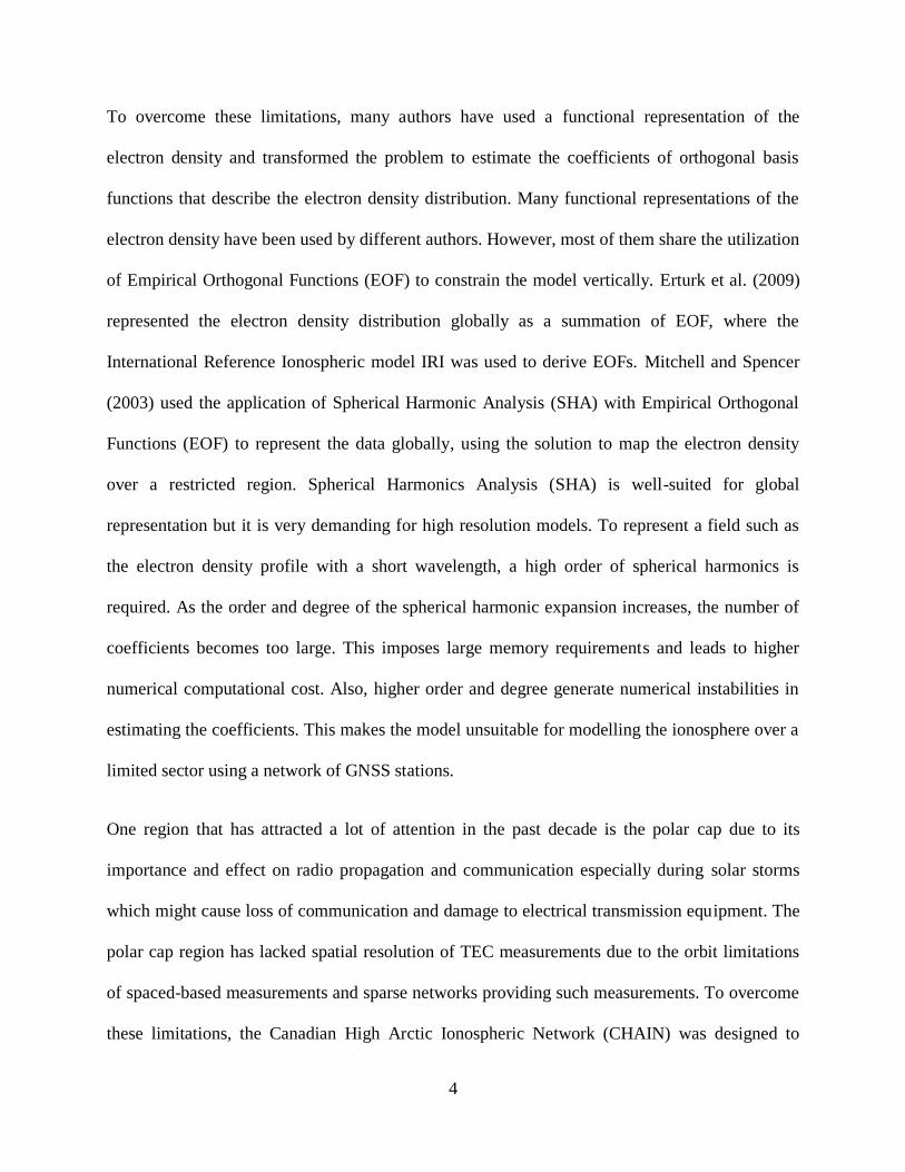
illustrated in Figure 2.1. This constellation ensures that almost all users with a clear sky view
have a minimum of four satellites in view, providing 24-hour global use for navigation.
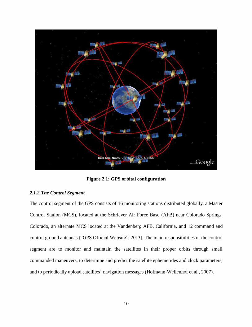
10
Figure 2.1: GPS orbital configuration
2.1.2 The Control Segment
The control segment of the GPS consists of 16 monitoring stations distributed globally, a Master
Control Station (MCS), located at the Schriever Air Force Base (AFB) near Colorado Springs,
Colorado, an alternate MCS located at the Vandenberg AFB, California, and 12 command and
control ground antennas (“GPS Official Website”, 2013). The main responsibilities of the control
segment are to monitor and maintain the satellites in their proper orbits through small
commanded maneuvers, to determine and predict the satellite ephemerides and clock parameters,
and to periodically upload satellites’ navigation messages (Hofmann-Wellenhof et al., 2007).
11
2.1.3 The User Segment
The user segment includes antennas and receivers of the military personnel and civilians which
collect and process measurements from the GPS satellites that are in view to compute local
position, velocity, and time. This process requires measurements from four satellites
simultaneously to compute a unique position solution (in three dimensions), in addition to the
receiver clock offset. With this capability, GPS has three main functions: navigation, precise
positioning, and time and frequency dissemination. The reference frame used by the GPS is the
World Geodetic System 1984 (WGS-84) which is a geocentric Earth-fixed system (Hofmann-
Wellenhof et al., 2007).
2.2 GPS Signal Structure
The legacy GPS signals are broadcast on two L-band frequencies: L1 = 1575.42 MHz and L2 =
1227.60 MHz. These signals are modulated by several codes with certain characteristics.
However, due to the increased need for improved accuracy and higher reliability, especially for
life safety applications, GPS is undergoing continuing modernization efforts with new signals
and bands. Since the number of satellites transmitting the modernized signals is limited, only
measurements from legacy GPS signals are used and described in this section.
The legacy L1 signal is modulated by two pseudorandom noise (PRN) codes: Coarse/Acquisition
code (C/A code) and Precise code (P-code). These codes consist of a digital sequence of random
bits (zeroes and ones) with special properties allowing satellites to transmit at the same
frequency without interfering with each other. The legacy L2 signal is modulated by the P-code
which is encrypted and intended for military users only. However, by using special signal
processing techniques in the receiver such as squaring and cross-correlation, measurement from
legacy L2 signal can be recovered for civilian use (Hofmann-Wellenhof et al., 2007).

12
C/A and P codes are repeated every 1 millisecond and 1 week, respectively, with chipping rates
of 1.023 MHz and 10.23 MHz, respectively. The difference in the chipping rate, hence chip
width (300 m for C/A code and 30 m for P-code), results in greater precision in the range
measurements for P-code than that for C/A-code. In addition to the pseudorandom codes, both
signals are modulated by a binary-coded message referred to as the navigation message which
contains data on the satellite health status, orbit and clock, and ionospheric corrections (Misra
and Enge, 2006). The navigation message is transmitted at a rate of 50 bits per second (bps) with
20 ms bit duration. Table 2.1 summarizes relevant components of the satellite signals.
Table 2.1: Components of the GPS satellite signal (after Hofmann-Wellenhof et al., 2007)
Component Frequency (MHz)
Fundamental frequency
Carrier L1
Carrier L2
P-code
C/A code
Navigation message
The L1 and L2 signals transmitted by the kth
satellite can be expressed mathematically as:
(2.1)
where:
, , and are signal powers for C/A code on L1 and P(Y) codes on L1 and L2
respectively (m)
13
and are the C/A and P(Y) code sequences of the kth
satellite
is the navigation data message of the kth
satellite
and are the carrier frequencies corresponding to L1 and L2 respectively (Hz)
and are the carrier phase offsets on L1 and L2 respectively (cycles)
In late 1990’s, GPS modernization was launched to expand the benefits of GPS for civil
applications. The project includes two new civil signals: L2C and L5. L2C signal is transmitted
on the L2 frequency, as L2 with two multiplexed PRN codes: Civilian Moderate length code
(CM) and Civilian Long length code (CL). The CM code has a length of 10,230 chips repeating
every 20 ms, and CL code has a length of 767,250 chips repeating every 1500 ms. Both codes
are transmitted at 511.5 kbit/s. However, they are multiplexed together to form the new code
L2C, which has the same 1.023 MHz chipping rate as the C/A codes. The L5 signal is
transmitted on the L5 frequency (1176.45 MHz) offering two carrier frequency components: in-
phase (I) and quadrature-phase (Q). The Q channel is a data-less channel, transmitting a pilot
signal modulated with a spreading code. The I channel is modulated with the navigation data and
a spreading code. Both codes are 10,230 chips in length and transmitted at 10.23 MHz, repeating
every 1 ms. Currently, there are ten satellites transmitting L2C signals and three satellites
transmitting L5 signals (“The United States Naval Observatory”, 2013).
2.3 GPS Observables
Generally, the Global Positioning System provides three observables: pseudorange, carrier
phase, and Doppler. A code tracking loop (delay lock loop) correlates the incoming signal with
replicas generated in the receiver to provide the apparent transit time of a signal from a satellite
to the receiver. Multiplication of the transit time by the speed of light in a vacuum results in
derivation of a pseudorange. A carrier phase tracking loop (phase lock loop) provides the phase

14
difference between the received signal and the sinusoidal signal generated by the receiver. The
time derivative of the carrier phase observation is the Doppler measurement. Ideally, the receiver
acquiring phase lock with the incoming signal would measure the initial fractional phase
difference between the received and receiver-generated signal plus the total number of full
carrier cycles between the satellite and the receiver. However, a GPS receiver cannot distinguish
between cycles of the received carrier wave. In reality, the receiver measures the fractional phase
and then keeps track of the changes in this measurement; the initial phase, which is an integer
number of full cycles referred to as carrier phase ambiguity ( ), is left undetermined. Estimation
of is referred to as integer ambiguity resolution.
2.4 GPS Error Sources
The carrier phase observable is more precise than the pseudorange but is ambiguous by the
carrier phase ambiguity. However, both measurements are subject to errors from various sources
which reduce the accuracy of GPS positioning. These errors can be grouped into satellite-based
errors (such as orbital errors and satellite clock errors), receiver-based errors (such as receiver
clock errors and noise), and signal propagation errors (such as ionospheric and tropospheric
delays and multipath). These errors are illustrated in Figure 2.2 and are included in the following
equations describing the pseudorange, carrier phase and Doppler observables:
(2.2)
(2.3)
(2.4)
where:
15
, are the code pseudorange (m), the carrier phase (m), and the Doppler
(m/s), respectively
is the carrier phase observable in cycles
is the carrier wavelength (m)
is the geometrical range between the receiver and the satellite (m)
is the geometrical range rate between the receiver and the satellite (m/s)
is the orbital error (m)
is the velocity error (m/s)
is the speed of light (m/s)
, are the satellite clock error (m) and clock drift error (m/s), respectively
, are the receiver clock error (m) and clock drift error (m/s), respectively
, are the tropospheric delay (m) and drift (m/s), respectively
, are the ionospheric delay (m) and drift (m/s), respectively
is the carrier phase ambiguity (cycles)
, are the satellite and receiver modulation offsets, respectively, which are
different for code versus carrier-phase (m)
is the random error due to receiver noise and multipath
is a subscript denoting GPS carrier frequencies
16
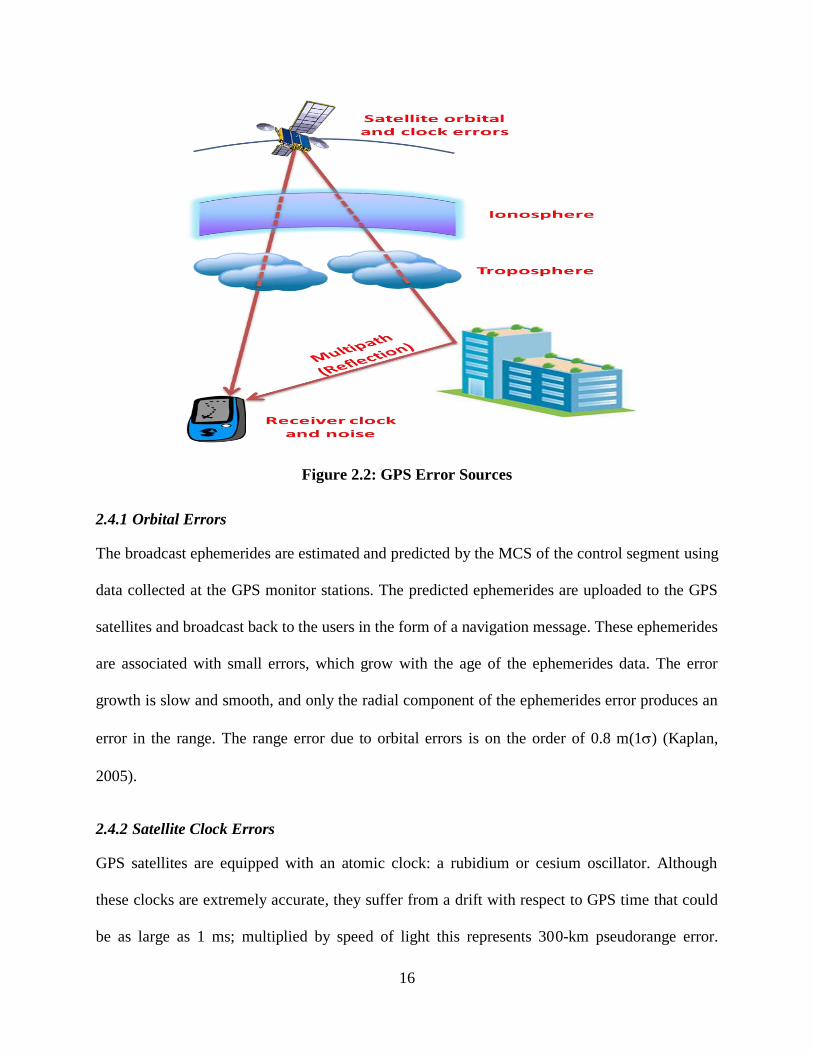
Figure 2.2: GPS Error Sources
2.4.1 Orbital Errors
The broadcast ephemerides are estimated and predicted by the MCS of the control segment using
data collected at the GPS monitor stations. The predicted ephemerides are uploaded to the GPS
satellites and broadcast back to the users in the form of a navigation message. These ephemerides
are associated with small errors, which grow with the age of the ephemerides data. The error
growth is slow and smooth, and only the radial component of the ephemerides error produces an
error in the range. The range error due to orbital errors is on the order of 0.8 m(1) (Kaplan,
2005).
2.4.2 Satellite Clock Errors
GPS satellites are equipped with an atomic clock: a rubidium or cesium oscillator. Although
these clocks are extremely accurate, they suffer from a drift with respect to GPS time that could
be as large as 1 ms; multiplied by speed of light this represents 300-km pseudorange error.
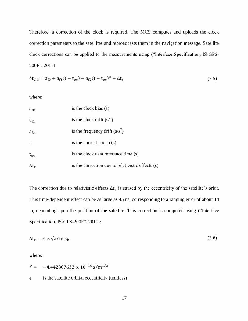
17
Therefore, a correction of the clock is required. The MCS computes and uploads the clock
correction parameters to the satellites and rebroadcasts them in the navigation message. Satellite
clock corrections can be applied to the measurements using (“Interface Specification, IS-GPS-
200F”, 2011):
(2.5)
where:
is the clock bias (s)
is the clock drift (s/s)
is the frequency drift (s/s2)
is the current epoch (s)
is the clock data reference time (s)
is the correction due to relativistic effects (s)
The correction due to relativistic effects is caused by the eccentricity of the satellite’s orbit.
This time-dependent effect can be as large as 45 ns, corresponding to a ranging error of about 14
m, depending upon the position of the satellite. This correction is computed using (“Interface
Specification, IS-GPS-200F”, 2011):
(2.6)
where:
is the satellite orbital eccentricity (unitless)
18
is the semi-major axis of the satellite orbit (m)
is the eccentric anomaly of the satellite orbit (radians)
The satellite clock error can be computed using Equations (2.5) and (2.6); however, some
residual error remains in the range 0.3-0.4 m of equivalent ranging error, depending on the age of
broadcast data and clock type (Kaplan, 2005).
2.4.3 Receiver Clock Errors
The receiver clock error (bias) is the difference between the time observed by the receiver
oscillator and the reference GPS time. This error varies with time and affects all range
measurements by the same amount for a fixed epoch. The receiver clock errors are higher than
the satellite clock errors since receivers use less expensive oscillators than those on satellites
such as low-cost quartz clock, temperature compensated crystal oscillator (TCXO), oven
controlled crystal oscillator (OCXO), or Rubidium oscillator. However, this time-varying error
can be estimated as an unknown along with the receiver position or eliminated by differencing
techniques.
2.4.4 Receiver Noise
The receiver noise error includes noise introduced by the antenna, amplifiers, cables, and the
receiver. The receiver is capable of measuring the phase with a precision of 1/2 % 1% of a
cycle; corresponding to ~2 mm. However, the noise level on the code measurement is much
higher, with typical errors of few decimeters (Misra and Enge, 2006).
19
2.4.5 Multipath
Multipath is the arrival of a signal at the receiver antenna via multiple paths. This phenomenon
results from the reflection of the signal from surfaces and structures in the vicinity such as
buildings, streets and vehicles, and from the ground. Multipath affects both pseudorange and
carrier phase measurements. Typical multipath errors in pseudorange measurements are on the
order of several metres, while the maximum multipath error on the carrier phase measurements
does not exceed a quarter cycle (Kaplan, 2005).
2.4.6 Tropospheric Errors
The troposphere is the lower part of the atmosphere, extending from the Earth’s surface to about
50 km altitude. The refractive index of the atmosphere is larger than unity, causing the speed of
propagation to be lower than that in free space and the signal to be delayed. This delay, referred
to as tropospheric delay, is a function of temperature, pressure and humidity and can be divided
into two parts: hydrostatic (dry) delay and wet delay. The hydrostatic delay is responsible for
90% of the tropospheric delay and can be accurately estimated using empirical models or surface
measurements. On the other hand, the wet delay, corresponding to 10% of the delay, is more
difficult to model due to the variation of water vapour in the lower atmosphere. The troposphere
is a non-dispersive medium at GPS frequencies; the tropospheric delay is frequency independent.
Both pseudorange and carrier phase measurements at L1 and L2 frequencies experience a
common tropospheric delay. Therefore, this delay cannot be derived using dual-frequency GPS
measurements, and tropospheric models (such as Saastamoinen and Hopfield models) must be
used to correct for this delay (Misra and Enge, 2006).
20
2.4.7 Ionospheric Errors
The ionosphere is the region of the atmosphere from about 60 km to more than 1500 km above
the Earth surface. The ionospheric delay is the main error source for GPS. The delay can vary
from a few meters to tens of meters depending on the solar cycle, hour of day, season,
geographic location and satellite elevation angle. The effect on pseudorange and carrier phase is
the same but opposite in sign; the carrier phase is advanced and the pseudorange is delayed. The
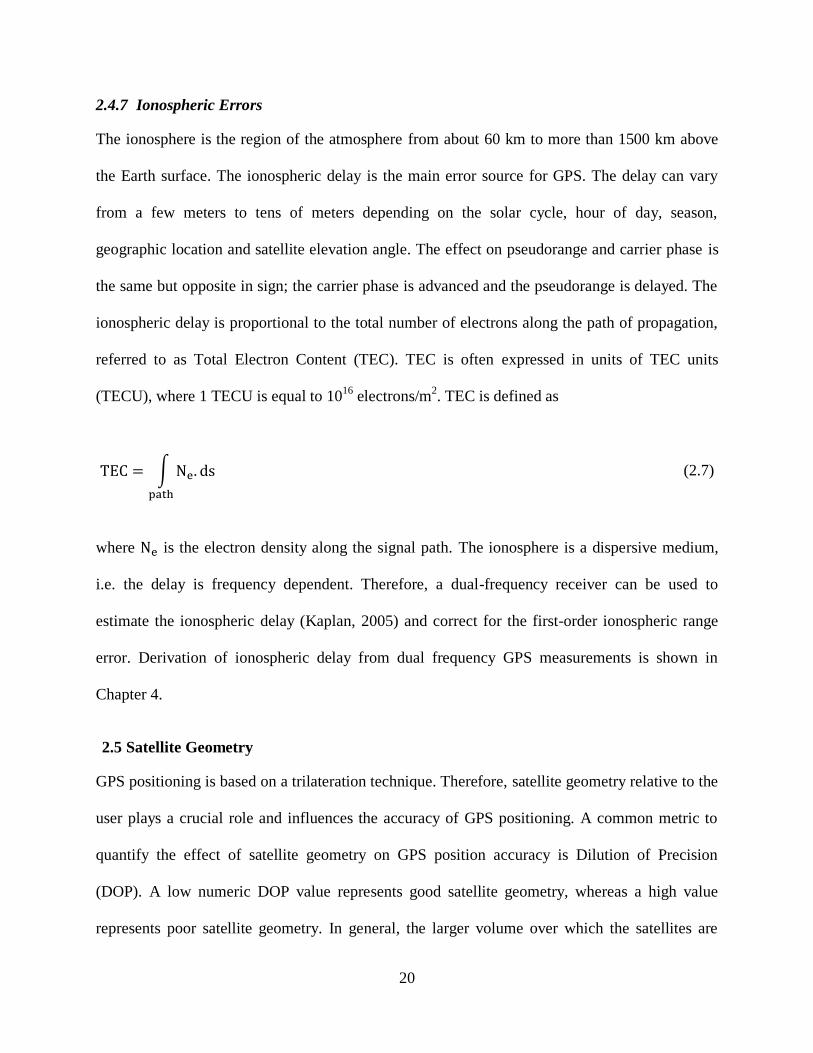
ionospheric delay is proportional to the total number of electrons along the path of propagation,
referred to as Total Electron Content (TEC). TEC is often expressed in units of TEC units
(TECU), where 1 TECU is equal to 1016
electrons/m2. TEC is defined as
(2.7)
where is the electron density along the signal path. The ionosphere is a dispersive medium,
i.e. the delay is frequency dependent. Therefore, a dual-frequency receiver can be used to
estimate the ionospheric delay (Kaplan, 2005) and correct for the first-order ionospheric range
error. Derivation of ionospheric delay from dual frequency GPS measurements is shown in
Chapter 4.
2.5 Satellite Geometry
GPS positioning is based on a trilateration technique. Therefore, satellite geometry relative to the
user plays a crucial role and influences the accuracy of GPS positioning. A common metric to
quantify the effect of satellite geometry on GPS position accuracy is Dilution of Precision
(DOP). A low numeric DOP value represents good satellite geometry, whereas a high value
represents poor satellite geometry. In general, the larger volume over which the satellites are

21
distributed the better the geometry. Figure 2.3 shows examples of good and poor satellite
geometry.
Figure 2.3: Good and poor satellite geometry
GPS positioning accuracy is a function of measurement accuracy as well as the satellite
geometry. The various errors described in the previous sections affect the GPS range observation
accuracy. This can be translated into position/time accuracy using the following rule-of-thumb:
(2.8)
Several DOP forms are used to describe the accuracy of position and time. This includes Position
Dilution of Precision (PDOP), Horizontal Dilution of Precision (HDOP), Vertical Dilution of
Precision (VDOP), and Time Dilution of Precision (TDOP). Geometric Dilution of Precision
(GDOP) is another useful form that characterizes the impact of the satellite geometry on the
position and time solution. Using these many DOP forms, the effect of satellite geometry on
estimating the position and time (GDOP), receiver 3D position (PDOP), horizontal position
22
(HDOP), vertical position (VDOP), easting position (EDOP), northing position (NDOP), and
receiver clock bias (TDOP) can be quantified using the following:
(2.9)
2.6 Differential GPS
Differential GPS (DGPS) is a technique that enhances the accuracy of GPS-derived position
solutions. This approach makes use of the fact that GPS measurements are spatially and
temporally correlated. This technique involves the use of reference stations at accurately known
locations. Collecting GPS measurements at the reference receivers, errors common to the remote
and reference receivers are estimated at the reference site and transmitted in a form of
corrections to the user. The user, in turn, applies these corrections to obtain a more accurate
position solution. Most of the errors discussed earlier can be mitigated except for noise and
multipath which are receiver and environment dependent and cannot be corrected using DGPS.

23
Figure 2.4: Differential GPS
Local-Area Differential GPS (LADGPS) and Wide-Area Differential GPS (WADGPS) are two
common forms of DGPS (Rao, 2010). In LADGPS, the reference receiver is generally located
within line-of-sight and the corrections sent to the user via a radio link account for ionospheric,
satellite clock, and ephemeris errors at the reference station. In WADGPS, the corrections are
determined using multiple reference stations distributed over a continent-wide geographic region
(Figure 2.5). Corrections are transmitted to the user in real time via geostationary satellite
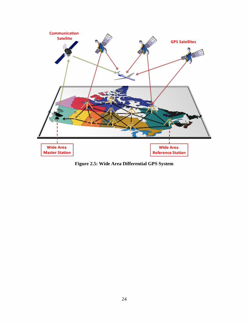
downlinks or through a network of ground based transmitters. Wide Area Augmentation System
(WAAS) (FAA, 2013) and European Geostationary Navigation Overlay Service (EGNOS)
(ESA, 2013) are examples of WADGPS.
24
Figure 2.5: Wide Area Differential GPS System
25
Chapter Three: The Ionosphere
The ionosphere is the part of the Earth’s atmosphere which extends from approximately 60 km to
more than 1500 km altitude. It results from the interaction of solar emissions (solar x-ray and
extreme ultraviolet radiation) with the Earth’s neutral atmosphere. This interaction controls the
ionization process, which in turn affects the electron production in the ionosphere. The evolution
of the ionosphere and its electron content varies in space and time (with solar cycle, seasonal,
and local time) and geographical location (low, mid, and high latitude, auroral and equatorial
regions) (Araujo-Pradere et al., 2005).
3.1 Structure of the Ionosphere
Ionization occurs at a number of atmospheric levels. It is mainly controlled by solar radiation and
solar activities. Having different compositions at different altitudes of the atmosphere, ionization
generates layers that may be identified by their interaction with radio waves. These layers are
shown in Figure 3.1 and described as follows:
Layer D: extends from 60 km to 90 km. This layer is generated by the hard X-radiation of
the sun, and the main effect of this layer is absorbing radiation. Due to the recombination
of ions and electrons, this region is reduced greatly after sunset.
Layer E: extends from 90 km to 140 km. Ionization (primarily of molecular oxygen) in
this layer is due to soft X-radiation of the sun and far ultraviolet solar radiation. This
layer is highly variable in space and time, where it is present during the day and reduced
by night. Sometimes, disturbances might occur in the ionosphere causing large
enhancements of electron density in some limited altitude range. When this feature
appears, a “Sporadic E” layer is said to be present.
26
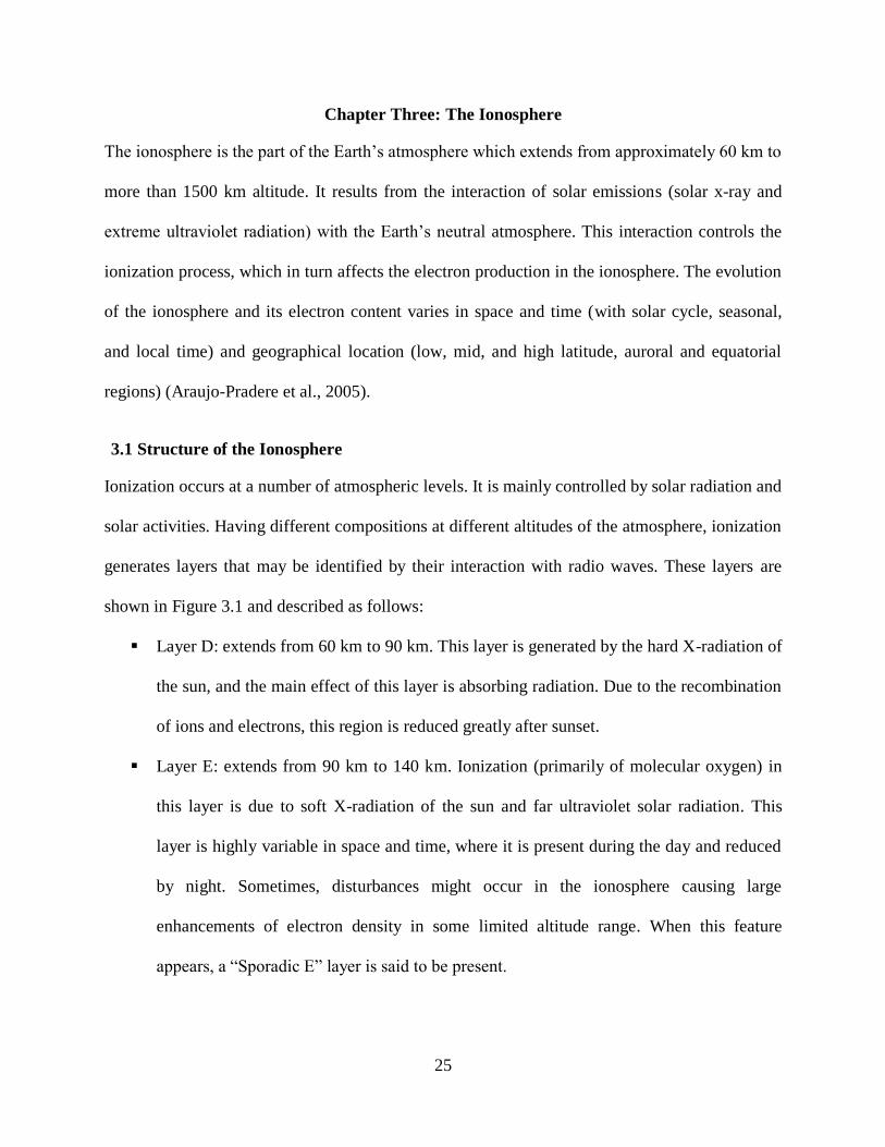
Layer F: extends from 140 km to 1000 km. Ionization of atomic oxygen (O) by extreme
ultraviolet solar radiation generates this layer. The F layer, also known as the Appleton
layer, is the highest significant layer of the ionosphere in terms of radio wave
communication. The central part of the F layer has the greatest electron density in the
Earth's atmosphere. This layer is divided into two sub-layers:
F1 Layer: extends from 140 km to 220 km altitude and only exists during
daytime. This is due to the nightside neutral wind which lifts the electrons, thus
the layer, to higher altitude.
F2 Layer: extends from 220 km to 1000 km altitude. This layer contains the
maximum value of the electron density profile at approximately 300 km altitude.
Figure 3.1: Ionospheric layers. at night, F1 and F2 layers combine into F layer and D layer
disappears

27
3.2 Ionospheric Characteristics
The ionospheric electron density an ionospheric characteristic of interest to GPS varies
spatially and temporally. Spatial variations are geographic position dependent while temporal
variations are Sun dependent. The following major electron density variations are briefly
discussed.
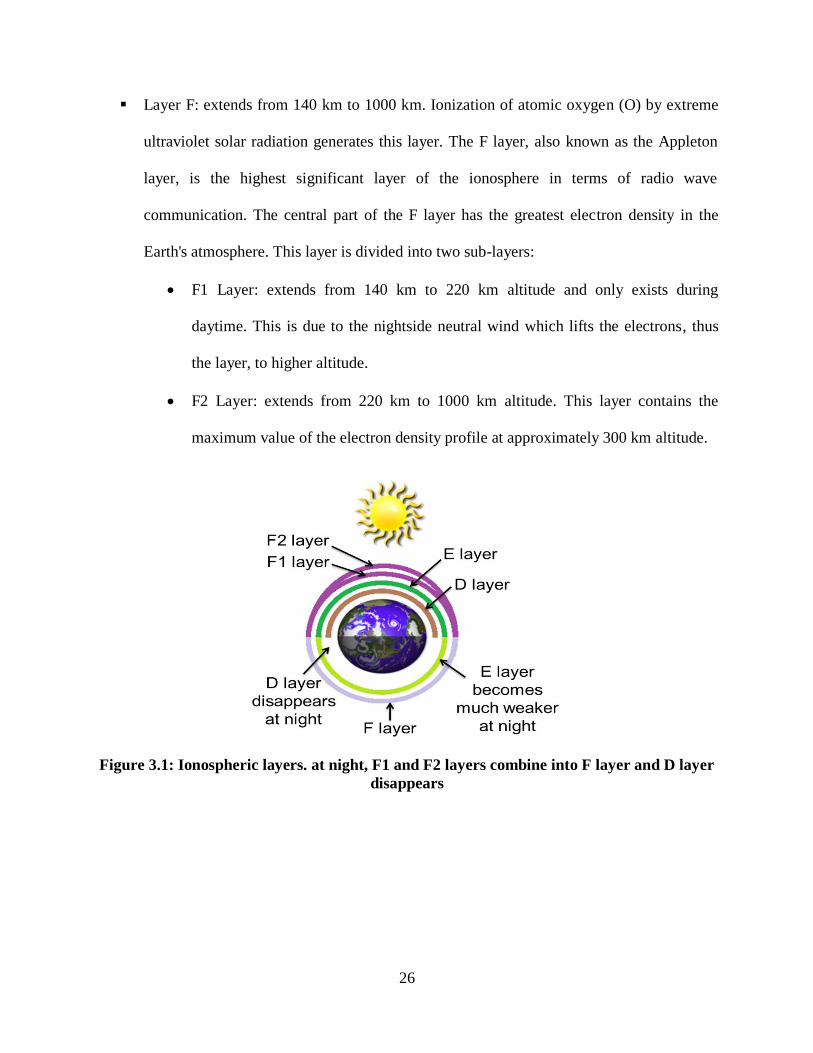
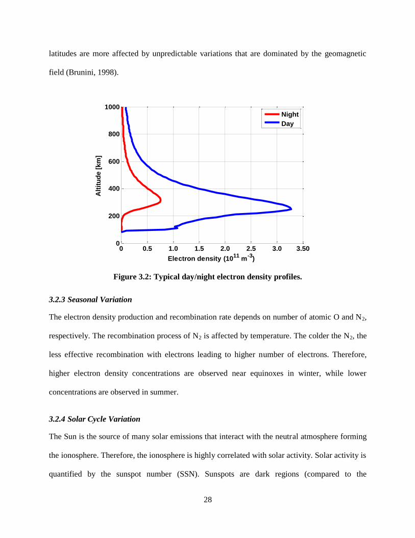
3.2.1 Diurnal Variation
The electron densities vary diurnally in an Earth-fixed reference frame. The rate of change of
electron density depends on the production rate, loss rate by recombination and transport
processes. The rate of ionization depends on solar radiation. Higher solar radiation intensity
leads to higher electron density. Figure 3.1 shows typical day/night electron density profiles.
During the day, the source of radiation, the Sun, stimulates the production of electron density. At
night, the recombination reaction is still in place but the source of radiation is removed causing a
decrease in the rate of ionization and hence decaying of the electron density. The electron density
reaches its maximum value at 1400 Local Time (LT) and has a minimum value at sunrise; the
dayside maximum is 4-6 times larger than the minimum values.
3.2.2 Latitudinal Variation
The ionosphere can be divided into three regions based on latitude: low-latitude (or equatorial)
region, mid-latitude region and high latitude (auroral and polar) region. In the low latitude
region, an equatorial anomaly develops near the geomagnetic equator. These anomalies are
caused indirectly by the neutral wind motions and by the combined action of ionospheric electric
and magnetic fields. The equatorial anomaly causes a minimum of electron density at the
magnetic equator and produces two peaks of electron density approximately 20º north and south
of the geomagnetic equator. In mid-latitudes the variations are more regular, but the high
28
latitudes are more affected by unpredictable variations that are dominated by the geomagnetic
field (Brunini, 1998).
Figure 3.2: Typical day/night electron density profiles.
3.2.3 Seasonal Variation
The electron density production and recombination rate depends on number of atomic O and N2,
respectively. The recombination process of N2 is affected by temperature. The colder the N2, the
less effective recombination with electrons leading to higher number of electrons. Therefore,
higher electron density concentrations are observed near equinoxes in winter, while lower
concentrations are observed in summer.
3.2.4 Solar Cycle Variation
The Sun is the source of many solar emissions that interact with the neutral atmosphere forming
the ionosphere. Therefore, the ionosphere is highly correlated with solar activity. Solar activity is
quantified by the sunspot number (SSN). Sunspots are dark regions (compared to the
0 0.5 1.0 1.5 2.0 2.5 3.0 3.500
200
400
600
800
1000
Alt
itu
de [
km
]
Electron density (1011
m-3
)
Night
Day

29
surrounding regions) on the photosphere of the sun, lying mainly between solar latitudes 5 and
30 caused by intense magnetic activity. The Sun exhibits an 11-year sunspot cycle, known as
the solar cycle. Figure 3.3 shows the solar cycle between 1954 and 2012. The strongest solar
cycle occurred in 1957 and the next peak is expected to occur in 2013-2014. During solar
maximum, the solar energetic emissions increase significantly affecting the ionosphere. These
emissions interact with the ionosphere releasing more electrons which in turn affect GPS
measurements.
Figure 3.3: Monthly and monthly smoothed sunspot numbers since 1954.
(http://sidc.oma.be/html/wolfmms.html, April 2013)

30
3.3 Ionospheric Models
3.3.1 Chapman Profile
The electron density profile in height can be described using a Chapman profile (Kelley, 2009).
Assuming hydrostatic equilibrium of a mass element with respect to the Earth’s surface and the
atmosphere approximation as an ideal gas, an expression for the electron density can be derived.
The final expression for a Chapman profile can be written as follows (Hargreaves, 1995):
(3.1)
where
, is the peak ionization rate, is the mean dissociative coefficient
for the molecular ions, and are the reference and scale heights respectively, and is the
sun zenith angle. Assuming a reference height ( ) of 300 km, a scale height ( ) of 75 km and
= 1012
el/m3, different profiles for different sun zenith angles ( ) are shown in Figure 3.4.
Figure 3.4: Different electron density profiles based on different sun zenith angles using
Chapman profile. (scale height = 75 km, reference height = 300 km, and = 1012
el/m3).

31
3.3.2 International Reference Ionosphere (IRI)
The International Reference Ionosphere (IRI) is an international scientific project sponsored by
the Committee on Space Research (COSPAR) and the International Union of Radio Science
(URSI). For a given location, time, date and sunspot number, the IRI model describes the median
values of electron density, the electron temperature, and ion composition in the altitude range 50
km to 2000 km. The major data sources for the IRI model are the worldwide network of
ionosondes, the powerful incoherent scatter radars, the International Satellites for Ionospheric
Studies (ISIS) and Alouette topside sounders, and in situ instruments on several satellites and
rockets (Bilitza and Reinisch, 2008).
3.3.3 Parameterized Ionospheric Model (PIM)
The Parameterized Ionospheric Model (PIM) is a global ionospheric and plasmaspheric model
based on combined output from the Global Theoretical Ionospheric Model (GTIM) model for
low and middle latitude with output from the Time Dependent Ionospheric Model (TDIM) for
high latitudes and from the empirical Gallagher plasmaspheric model (AIAA, 1999). PIM
produces electron density profiles between 90 and 25000 km altitude, in addition to other profile
parameters such as corresponding critical frequencies and heights for the ionospheric E and F2
regions, and Total Electron Content (TEC) (Daniell et al., 1995). Figure 3.5 is an example of a
profile for the same geographical coordinates and epoch using IRI-2007 and PIM models.

32
Figure 3.5: IRI-2007 and PIM profiles (Calgary, Canada 51.05° N, 114.07° W) .
3.4 Ionospheric Effects on GPS Signals
Electromagnetic signals propagating from a GPS satellite to a GPS receiver on the Earth’s
surface travel through the ionized layer of the atmosphere, i.e. the ionosphere. The ionosphere is
a dispersive medium with respect to the GPS signal: the refractive index, and hence the
ionospheric delay, is a function of the carrier frequency. In deriving the GPS observables it is
assumed that the signal travels at speed of light in a vacuum (index of refraction is equal to one).
Due to the ionospheric refractive index differing from a value of one, GPS signals are
significantly affected by the ionosphere, in terms of modifying the traveling speed of the signal
with respect to the speed of light. This induces two effects: 1) group delay of the signal

33
modulation and 2) carrier phase advance. The following expression relates the phase ( ) and the
group ( ) indices of refraction (Hofman-Wellenhof et al., 2001):
(3.2)
where is the system operating frequency, in Hz. According to Seeber (2003), the phase
refractive index ( ) can be approximated by truncating the series expansion after the quadratic
term:
(3.3)
Differentiating Equation (3.3)
(3.4)
And by substituting Equations (3.4) and (3.3) into Equation (3.2), an expression for the group
index of refraction can be derived:
(3.5)
The value does not depend on frequency but on the quantity of the electron density and is
defined as (Seeber, 2003)
where (3.6)
On the other hand, the measured range between a transmitter and a receiver can be defined using
Fermat’s principle:

34
(3.7)
Assuming =1, the geometric range is obtained:
(3.8)
The difference ( ) between measured range and geometric range is called ionospheric delay:
(3.9)
Since there are two refractive indices for the ionosphere, one for phase and the other for group,
there will be an ionospheric range error associated with each index. Substituting Equations (3.3)
and (3.5) into Equation (3.9) results in the following range errors:
(3.10)
Defining the Slant Total Electron Content ( ) as the integration of the electron density
along the signal path:
(3.11)
and substituting Equation (3.11) into Equation (3.10) yields:
(3.12)
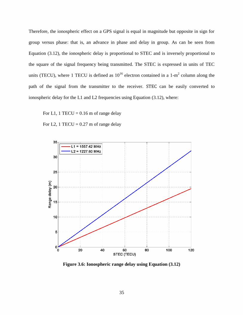
35
Therefore, the ionospheric effect on a GPS signal is equal in magnitude but opposite in sign for
group versus phase: that is, an advance in phase and delay in group. As can be seen from
Equation (3.12), the ionospheric delay is proportional to STEC and is inversely proportional to
the square of the signal frequency being transmitted. The STEC is expressed in units of TEC
units (TECU), where 1 TECU is defined as 1016
electron contained in a 1-m2 column along the
path of the signal from the transmitter to the receiver. can be easily converted to
ionospheric delay for the L1 and L2 frequencies using Equation (3.12), where:
For L1, 1 TECU = 0.16 m of range delay
For L2, 1 TECU = 0.27 m of range delay
Figure 3.6: Ionospheric range delay using Equation (3.12)
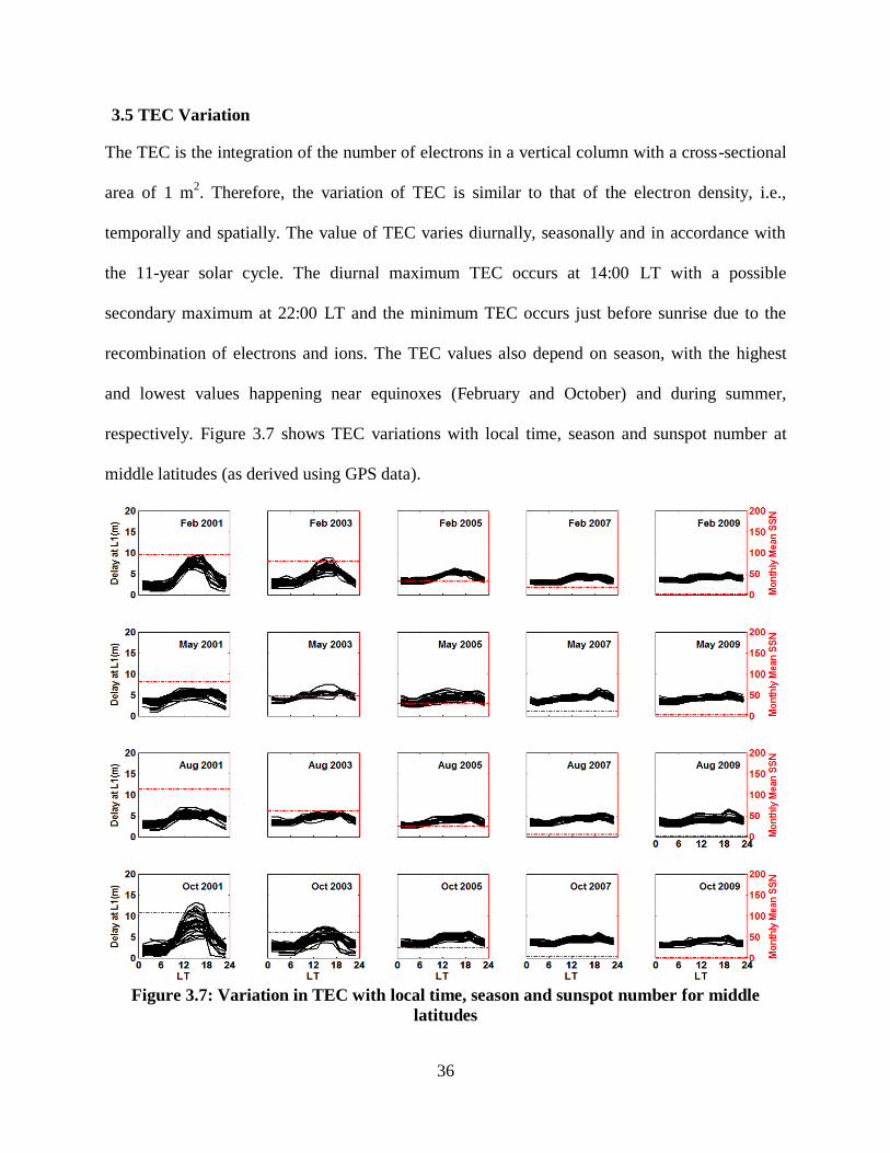
36
3.5 TEC Variation
The TEC is the integration of the number of electrons in a vertical column with a cross-sectional
area of 1 m2. Therefore, the variation of TEC is similar to that of the electron density, i.e.,
temporally and spatially. The value of TEC varies diurnally, seasonally and in accordance with
the 11-year solar cycle. The diurnal maximum TEC occurs at 14:00 LT with a possible
secondary maximum at 22:00 LT and the minimum TEC occurs just before sunrise due to the
recombination of electrons and ions. The TEC values also depend on season, with the highest
and lowest values happening near equinoxes (February and October) and during summer,
respectively. Figure 3.7 shows TEC variations with local time, season and sunspot number at
middle latitudes (as derived using GPS data).
Figure 3.7: Variation in TEC with local time, season and sunspot number for middle
latitudes

37
Figure 3.8 shows an example of how a network of GNSS receivers can be used to map the
ionosphere. This map represents the global variation of TEC values. During nominal ionospheric
conditions the TEC values are maximum near the equator – equatorial anomaly – and decrease
with increasing latitude.
Figure 3.8: Global Ionospheric Map (GIM) (data courtesy of CODE)
During geomagnetically disturbed periods, the electrons in the ionosphere may increase
especially near the mid-to-high latitudes and an enhancement of ionospheric TEC occurs. These
electrons are carried from lower latitudes to high latitudes forming a plume of enhanced TEC.
This phenomenon is referred to as Storm Enhanced Density (SED). SED was first identified in
the early 1990’s with the Millstone incoherent scatter radar (Foster, 1993) and has been observed
and reported over North America (Coster and Skone, 2009) and Europe (Coster et al., 2007). An
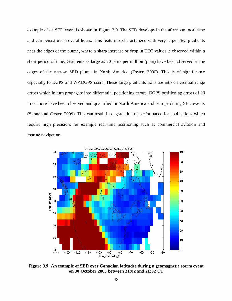
38
example of an SED event is shown in Figure 3.9. The SED develops in the afternoon local time
and can persist over several hours. This feature is characterized with very large TEC gradients
near the edges of the plume, where a sharp increase or drop in TEC values is observed within a
short period of time. Gradients as large as 70 parts per million (ppm) have been observed at the
edges of the narrow SED plume in North America (Foster, 2000). This is of significance
especially to DGPS and WADGPS users. These large gradients translate into differential range
errors which in turn propagate into differential positioning errors. DGPS positioning errors of 20
m or more have been observed and quantified in North America and Europe during SED events
(Skone and Coster, 2009). This can result in degradation of performance for applications which
require high precision: for example real-time positioning such as commercial aviation and
marine navigation.
Figure 3.9: An example of SED over Canadian latitudes during a geomagnetic storm event
on 30 October 2003 between 21:02 and 21:32 UT

39
Chapter Four: Ionospheric Tomography
4.1 Introduction
Tomography is defined as cross-sectional imaging of an object from either transmitted or
reflected data collected by illuminating the object from many different directions and
orientations. This method has been used in medicine, geophysics, biology and many other
sciences. It consists of reconstruction of an image from the integrals of that image in multiple
directions. Ionospheric tomography was first proposed by Austen et al. (1986), and it has
received a lot of attention in the past two decades due to its capabilities of monitoring and
detecting irregularities in the ionosphere. Further improvements were performed and different
methodologies were implemented by many authors (Mitchell and Spencer, 2003; Raymund et al.,
1993).
4.2 Tomography Problem
The following example illustrates the tomography problem. For simplicity, a two-dimensional
projection is shown in Figure 4.1, where four homogeneous blocks with sides of unit length and
assigned parameters are intersected by six ray paths. Each measurement is simply the integration
of the assigned parameters along the measurement path from the transmitter to the receiver.
Approximating integration with a summation, the measurement can be considered as the sum of
the path lengths in each pixel multiplied by the unknown parameter in the pixel. The problem of
tomography is to determine the unknown parameter (such as electron density) from the set of
path-integrated measurements (such as STEC).
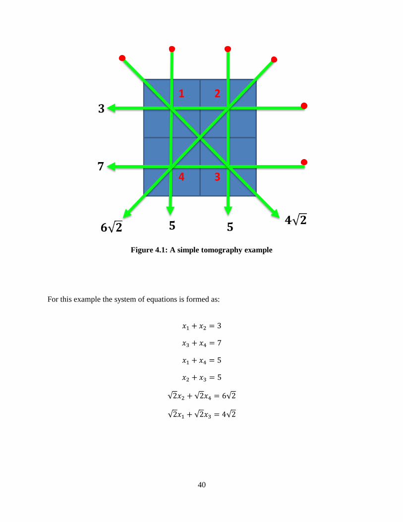
40
Figure 4.1: A simple tomography example
For this example the system of equations is formed as:
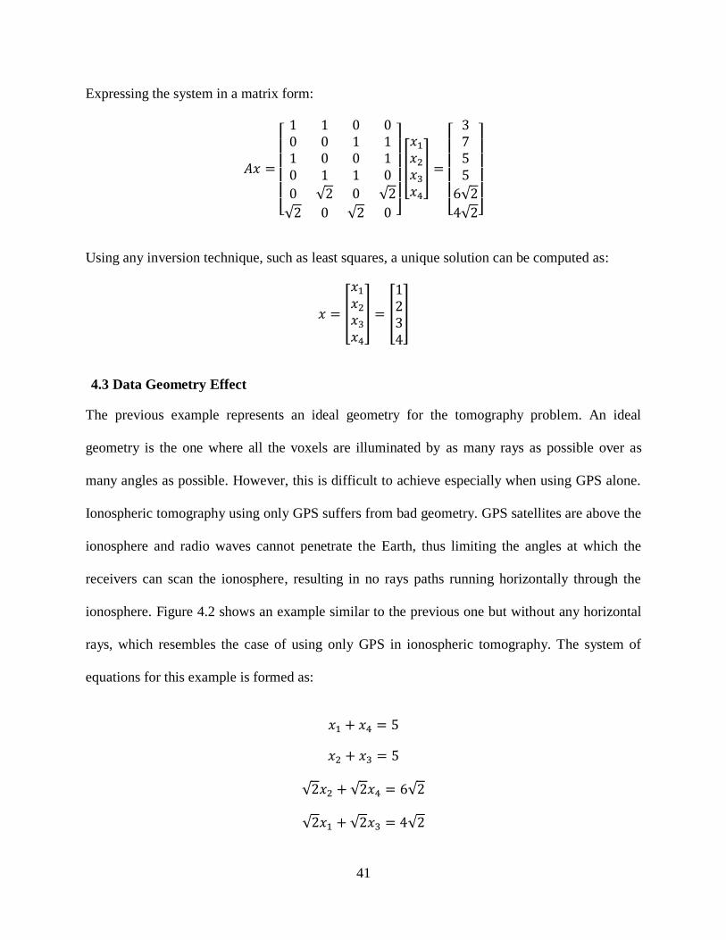
41
Expressing the system in a matrix form:
Using any inversion technique, such as least squares, a unique solution can be computed as:
4.3 Data Geometry Effect
The previous example represents an ideal geometry for the tomography problem. An ideal
geometry is the one where all the voxels are illuminated by as many rays as possible over as
many angles as possible. However, this is difficult to achieve especially when using GPS alone.
Ionospheric tomography using only GPS suffers from bad geometry. GPS satellites are above the
ionosphere and radio waves cannot penetrate the Earth, thus limiting the angles at which the
receivers can scan the ionosphere, resulting in no rays paths running horizontally through the
ionosphere. Figure 4.2 shows an example similar to the previous one but without any horizontal
rays, which resembles the case of using only GPS in ionospheric tomography. The system of
equations for this example is formed as:

42
Figure 4.2: Effect of data geometry on tomography
Expressing the system in a matrix form:
Although all pixels (voxels in two dimensions) are illuminated by two ray paths, this problem
has an infinite number of solutions (determinant of matrix A = 0). and
are two possible solutions that satisfy the above system of equations. In
addition to these solutions, there can be found an infinite number of possible solutions. This
example shows the effect of non-ideal data geometry on the existence and uniqueness of the
solution. This problem is intensified when the model is extended to three dimensions. Therefore,
a different approach is required to minimize the effect of bad data geometry on the uniqueness
and existence of the solution, especially in the case of using only GPS measurements. The
43
following section summarizes the development of ionospheric tomography to overcome the
effect of bad data geometry and solve the ionospheric problem and highlights some of the
technique’s limitations.
4.4 Overview of Ionospheric Tomography Development
Ionospheric imaging was first applied in two dimensions. Iterative techniques were the first
choice to be used to solve the ionospheric tomography problem due to their simplicity and low
memory requirement. Austen et al. (1986) presented the theory of Computerized Ionospheric
Tomography (CIT) and the application of Algebraic Reconstruction Technique (ART) to the
problem of ionospheric imaging. Afraimovich et al. (1992) and Pryse and Kersley (1992)
reported results of ionospheric tomography using Simultaneous Iterative Reconstruction
Technique (SIRT). Raymund et al. (1993) applied Multiplicative Algebraic Reconstruction
Technique (MART) algorithm to a Scandinavian campaign in September 1991. All their results
showed that iterative techniques could retrieve the electron distribution given a good initial
guess. However, some concerns and limitations were identified: noise and initial guess.
Noise and initial guess affect the reconstruction significantly. A proper choice of relaxation
parameter can reduce the effect of noise but affect the number of iterations required. Austen et al.
(1986) showed that the number of iterations increased as the relaxation parameter was reduced.
Also, choosing an initial guess is important in iterative technique. A good guess compensates for
the incomplete information in the measurements. Therefore, a good initial guess (known as a
background ionosphere) has been introduced and used in iterative techniques. Raymund et al.
(1993) used a two-step procedure, where the background ionosphere was reconstructed first
using IRI-90 then used as the initial guess to MART technique.
44
To overcome the limitations of iterative techniques, stochastic inversion techniques were used
and applied by many authors (Fremouw et al., 1992). Because of the limited number of
measurements and poor geometry of the ionospheric tomography problem, many approaches
were developed to compensate for the missing information and singularity of the design matrix.
Bhuyan et al. (2002) presented and discussed the development of a new algorithm based on
Generalized Singular Value Decomposition (GSVD). Meggs et al. (2004) implemented the so-
called full inversion method and compared it to a single shell grid model. Results showed that for
mid- to high-latitudes the inversion method was better than the single shell or at least similar to it
in some cases. Bhuyan et al (2004) extended the investigation of applying GSVD and
regularizing (imposing additional information or constraints to solve ill-posed problems) the
ionospheric tomography problem. The effect of geometry was investigated by increasing the
number of sampling rays within the same latitude range. As a result, the solution gave a very
good reconstructed image with poor reconstruction only near the edges of the image. Also,
results showed that when irregularities are present the first order regularization is optimum and
higher order methods had a much stronger smoothing effect which tends to hide important
features of the image during highly disturbed ionospheric conditions. This is due to the fact that
the first order regularization is a differencing (averaging) operator. The second order is the
derivative of the differencing operator, which results in smoother values. Therefore, the higher
the order is, the strongest the smoothing effect.
It should be mentioned that early results were based on real and/or simulated data of the Navy
Navigation Satellite System (NNSS). Having these satellites in Low-Earth Orbits (LEOs), the
ionosphere was often considered temporally static during a satellite pass and only two-
dimensional images (altitude vs. latitude) of the ionosphere were produced since the ground
45
receivers of NNSS were often installed along a fixed longitude chain cross section. With such
LEO TEC data, only regional images could be produced with a low number of passes per day to
a receiver array. Therefore, two-dimensional LEO tomography is limited both spatially and
temporally. On the other hand, the development of GPS offered a new source of TEC data,
especially after Selective Availability (SA) was turned off in May 2000. First experimental
results using GPS data in ionospheric tomography were demonstrated in Rius et al. (1997) . This
work was the first step to advance from the conventional 2-D imaging into 3-D ionospheric
tomography using GPS.
Three dimensional imaging is based on the same observations as two dimensional imaging but is
more complex in parameter estimation. The data are sparse and the data geometry is often not
ideal. Therefore, iterative techniques are not the best choice since they do not incorporate any
information from the surrounding voxels to the voxel with no measurement intersection. As a
result a new method has been proposed to overcome such limitations. The method compensates
for the missing ionospheric information in many voxels by adding physically reasonable
constraints representing a realistic ionosphere. This can be achieved using orthonormal basis
functions derived from empirical ionospheric models such as PIM and IRI. The idea of
constraining the electron density profile using Empirical Orthogonal Functions (EOF) was taken
from Fremouw et al. (1992) and adopted by many authors in their models with some
modifications (Erturk et al., 2009; Liu and Gao, 2004; Mitchell and Spencer, 2003; Schmidt,
2007; and many others).
All of the above methods considered the ionosphere temporally static. This assumption is an
approximation of reality as the ionosphere is a highly variable medium. Therefore, it is important
to accommodate the temporal changes in the images. Several authors (Mitchell and Spencer,

46
2003; Rius et al., 1997; Schmidt, 2007) extended the model to accommodate temporal changes in
the images. Mitchell and Spencer (2003) used simulated ground-GPS data from actual
measurement geometry over Europe and inverted TEC data to evaluate the underlying
distribution and time evolution of the electron concentration. Results showed an accurate
representation (no worse than 1 TECU error) of the zonal and meridional gradients and slight
underestimation of vertical TEC on the order of 1 percent.
The extension of ionospheric imaging from two dimensions into three and four dimensions (time
being the fourth dimension) has been implemented. IDA3D (Bust et al., 2004) and MIDAS
(Mitchell and Spencer, 2003) are examples of such implementation. MIDAS is a linear inversion
tomographic technique that uses orthogonal functions to constrain the electron density profile
and spherical harmonics to describe the electron density profile horizontally. However, a high
order and degree of spherical harmonics are required to recover the spatial resolution of electron
density over a wide area. This will lead to some difficulties inverting the problem, especially in
areas with limited GPS stations as in the Canadian polar region.
As will be shown later, when the electron density field wavelength decreases, a higher order and
degree of spherical harmonics are required to represent the field. Using higher order and degree
leads to a larger number of unknowns which, in turn, makes the numerical cost expensive and the
problem more susceptible to round-off errors (especially given that ionospheric tomography is
nearly singular and ill-conditioned). Also, having a larger number of coefficients makes
broadcasting them to single-frequency GPS users and using them in near real time difficult. The
computational load associated with this number at the user end is significant. Therefore, a more
suitable functional representation of the electron density over the Canadian polar region is
required. This representation should be able to describe the minimum representable wavelength
47
with a lower number of coefficients (unknowns) than those used in other techniques. Potentially,
these coefficients can be broadcast to single-frequency GPS users to apply any necessary
ionospheric corrections. The following sections describe the development of the model starting
from the observation to the functional representation of the electron density profile in three
dimensions.
4.5 Extracting Ionospheric Information from GPS Observables
In an ionospheric context, the electron density corresponds to the cross-sectional image. To
reconstruct that image, integrals of the image in different directions and orientations are needed.
According to Equation (3.11), is the integral of the electron density along the satellite-
receiver Line-of-Sight (LOS). Once the transmitter and receiver coordinates are known, is
used to reconstruct using tomography. In cases where GPS is used, can be derived
using dual frequency GPS observations.
4.5.1 STEC Observation
The “geometry-free” linear combination of GPS observations is used to derive the
observable. The geometric range, clock-offsets and tropospheric delay are frequency independent
and can be eliminated using this combination. The “geometry-free” linear combinations for
pseudorange and carrier phase observations are given as (Kleusberg and Teunissen, 1998):
(4.1)
(4.2)
where
, are ionospheric delays on L1 and L2 pseudoranges (m)
, are the carrier wavelengths

48
, are the carrier phase ambiguities
is the receiver code-delay Inter-Frequency Bias (IFB) (m)
is the satellite code-delay IFB (m)
is the receiver IFB (m)
is the satellite IFB (m)
is the combination of multipath and measurement noise on
and (m)
is the combination of multipath and measurement noise on
and (m)
Substituting Equation (3.12) in Equation (4.1),
(4.3)
and rearranging Equation (4.3), the relative can be derived as
(4.4)
where
is the receiver code-delay IFB in TECU
is the satellite code-delay IFB in TECU
is the combination of multipath and measurement noise on
and in TECU
49
The relative can be derived from the phase measurements using the same approach:
(4.5)
where
is the receiver IFB in TECU
is the satellite IFB in TECU
is the combination of multipath and measurement noise on
and in TECU
is the bias in the ionospheric observable due to carrier phase
ambiguities on and
4.5.2 STEC Smoothing
Pseudorange measurements are subject to high noise and multipath effects. As a result, the code-
derived observation is noisy. The multipath effect can be mitigated using an RF-
absorbing ground plane or choke-ring at the antenna. The effect can also be reduced in the
receiver where advanced receiver technologies have been developed and implemented (Misra
and Enge, 2006). To reduce the multipath and noise level in the observables, the carrier
phase measurements are used to compute a more precise relative observable. Although the
50
carrier-phase derived observables are more precise than the code-derived , they are
ambiguous due to the presence of integer phase ambiguities in the carrier phase measurements.
To take advantage of the low-noise carrier phase derived and unambiguous nature of the
code-derived , both measurements are combined and is smoothed using the
"levelling" process (Ciraolo et al., 2007). In this approach, the continuous arcs of are
adjusted to the mean value of the corresponding code value. The mean value is computed
for every continuous arc using:
(4.6)
where is the number of continuous measurements contained in the arc and denotes the
mean value. Assuming constant IFBs and substituting Equations (4.4) and (4.5) in Equation
(4.6):
(4.7)
The noise and multipath levels on the geometry-free combination derived from carrier phase
measurements are much smaller than those derived from pseudorange
measurements . Therefore, the noise and multipath term for the carrier phase has
been neglected in Equation (4.7). Subtracting Equation (4.5) from (4.7), the ambiguity terms can
be eliminated and the smoothed can be derived:
(4.8)
Figure 4.3 illustrates the STEC smoothing algorithm for PRN 7 using Equation (4.8). It can be
seen that contains larger noise than .

51
Figure 4.3: Comparison of code-derived (STECP ), phase-derived (STEC ) and smoothed
STEC (STECsmoothed ) calculated along the slant signal path of GPS satellite 7 observed
from ALGO on January 1, 2010.
Equation (4.8) assumes that the carrier phase ambiguity terms and remain constant
throughout the observation period. In other words, the carrier phase observations should not be
affected by cycle slips, i.e., discontinuity of an integer number of cycles in the carrier phase
observations. Therefore, cycle slip detection must be performed for every epoch and cycle slips
corrected when possible. In case a detected cycle slip could not be corrected, the smoothing
algorithm must be reinitialized.
52
4.5.3 Cycle Slip Detection
The receiver carrier phase tracking loop records two components: integer component and
fractional component. When a GPS receiver is tracking a signal, the integer component is
initialized to an arbitrary integer number of cycles (i.e. carrier phase ambiguity) and the receiver
keeps track of the number of full cycles afterward. Adding the full number of cycles to the
fractional component, a carrier phase measurement is formed and reported. If the receiver loses
phase lock, the integer component is reinitialized causing a sudden jump in the carrier phase
observable by an integer number of cycles, known as cycle slip. Occurrence of cycle slips does
not affect the fractional component of the carrier phase. Cycle slips result from a temporary loss
of lock in the carrier tracking loop of a GPS receiver, due to obstructions of the satellite signal
caused by trees, buildings…etc., degraded signal to noise (SNR) due to low elevation
observations and active ionospheric conditions, multipath and higher receiver dynamics. Cycle
slips may occur between two epochs or may last several minutes or more, and their magnitude
may range from few cycles to millions of cycles (Seeber, 2003).
In order to derive continuous series of smoothed using Equation (4.8), cycle slips in the
carrier phase measurement used to derive must be detected and corrected, if possible. In
this research, two methods are used to detect cycle slips: wide lane and geometry-free detection
criteria (Sharma et al., 2011).
The wide lane phase combination is formed as follows:
(4.9)
where the wide lane wavelength is

53
(4.10)
In order to eliminate the common non-dispersive delays and ionospheric terms, the narrow lane
pseudorange combination is used:
(4.11)
and the widelane ambiguity terms is isolated as follows:
(4.12)
Equation (4.12) is highly affected by the multipath and noise propagated through
combination, which makes the cycle slip more difficult to detect especially under large
multipath. A cycle slip is detected if the following condition is satisfied
(4.13)
where denotes the mean value, and
(4.14)
(4.15)
is an arbitrary threshold factor that depends on assumed magnitudes of multipath and receiver
noise. The lower the threshold is, the more sensitive the detection method is, and therefore this
value must be chosen carefully. Optimal threshold factors range from 4 to 6.
The wide lane cycle slip detection method is based on the assumption that there are no identical
cycle slips occurring on L1 and L2 simultaneously. In such cases, an alternative criterion, the

54
geometry-free detection criterion, is used, where Equations (4.1) and (4.2) are used and the
geometry-free bias is formed:
(4.16)
is expected to remain constant over time in the absence of a cycle slip. However, this bias is
corrupted by multipath and noise, and the same algorithm used for the wide line combination is
adopted:
(4.17)
where
(4.18)
(4.19)
4.6 Model Development
The following subsections describe the development of the CIT technique proposed to
reconstruct the electron density over the Canadian polar region.
4.6.1 Voxel-Based Model
Figure 4.4 shows the geometry involved in ionospheric tomography. GPS satellites orbit at an
altitude of ~20,200 km, which is above the ionosphere. As these satellites transmit high
frequency electromagnetic radio waves, GPS receivers located on the Earth’s surface collect
observations that are affected by the ionosphere. Working with high frequency radio waves,
bending due to the ionosphere is considered negligible and the signal path from the satellite to
the receiver is assumed to be a straight line.
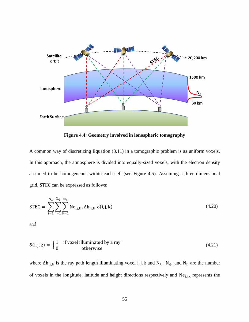
55
Figure 4.4: Geometry involved in ionospheric tomography
A common way of discretizing Equation (3.11) in a tomographic problem is as uniform voxels.
In this approach, the atmosphere is divided into equally-sized voxels, with the electron density
assumed to be homogeneous within each cell (see Figure 4.5). Assuming a three-dimensional
grid, can be expressed as follows:
(4.20)
and
(4.21)
where is the ray path length illuminating voxel and , ,and are the number
of voxels in the longitude, latitude and height directions respectively and represents the
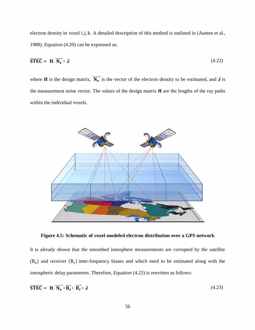
56
electron density in voxel . A detailed description of this method is outlined in (Austen et al.,
1988). Equation (4.20) can be expressed as:
(4.22)
where is the design matrix, is the vector of the electron density to be estimated, and is
the measurement noise vector. The values of the design matrix are the lengths of the ray paths
within the individual voxels.
Figure 4.5: Schematic of voxel-modeled electron distribution over a GPS network
It is already shown that the smoothed ionosphere measurements are corrupted by the satellite
( and receiver inter-frequency biases and which need to be estimated along with the
ionospheric delay parameters. Therefore, Equation (4.22) is rewritten as follows:
(4.23)
57
Equation (4.23) cannot be solved directly using ordinary stochastic techniques because the
observation geometry is not ideal and the design matrix is nearly singular and incorporates no
prior information to the solution. To overcome this problem, a reduction of unknowns is
required. This can be done by eliminating the biases using the relative changes of STEC along
continuous satellite-receiver LOS. Thus, taking a certain reference measurement, usually the
first, within an arc, the design matrix H and the measurement vector are differenced with
respect to the reference measurement. As a result, the ionospheric tomography problem can be
expressed as follows:
(4.24)
However, the design matrix in Equation (4.24) is underdetermined and ill-conditioned;
therefore, a straight solution of this inversion problem must be done in a different way.
Transformation of the problem to another space can be applied to overcome this problem, where
the unknowns are coefficients of three-dimensional orthonormal basis functions (Mitchell and
Spencer, 2003). The mapping matrix used in this transformation is generated using a spherical
harmonic expansion and EOF to represent the horizontal and vertical variation in electron
concentration, respectively, allowing a certain range of possible solutions. A priori information is
needed to generate the mapping function. However, the choice of the vertical profile set to form
the basis functions is a critical factor in the accuracy of the solution. Results presented in
(Mitchell and Spencer, 2003) showed an underestimation of TEC due to the limited number of
EOFs used in the inversion.

58
4.6.1.1 Design of 3-D Voxel-Based Model
The values of and of Equation (4.20) are required to construct the design matrix
H used in the voxel-based model. These values are computed using the following procedure:
Form the equation of LOS from the satellite to the receiver.
Find the equations of each side (6 sides) of each voxel.
Find points of intersection of LOS with each side of each voxel:
o If the LOS illuminates voxel , then is set to 1 and two points of
intersection exist, or 0 otherwise.
o Once is set to 1, is computed as the distance between the two points of
intersection.
Starting with the first step, given the satellite coordinates P1 and the station coordinates Po, the
LOS equation is formed as follows:
(4.25)
Figure 4.6 shows the definition of the voxel sides and its representation with respect to the
Earth’s surface. The top and bottom sides are parallel to the Earth’s surface, which is described
by a sphere. The equation describing the spherical surface at each height is governed by:
(4.26)
where is the Earth's radius. The North and South sides are described by a conic surface,
according to:
(4.27)
59
where is the latitude. Finally, the East and West sides are parallel to two great circles passing
through the two longitudes that define the voxel boundaries along the longitudinal direction. The
relationship between the and coordinates is described by:
(4.28)
Substituting Equation (4.25) in the equation of each side and solving for the value of (t), the
point of intersection of the LOS with each side, if it exists, is computed by substituting (t) in
Equation (4.25).

60
(a) voxel top and bottom sides
(b) voxel front and back sides
(c) voxel left and right sides
Figure 4.6: Voxel sides definition
Top side
South side
North side
East side
Bottom side
West side
Side
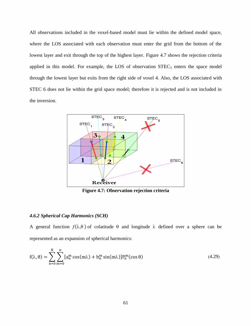
61
All observations included in the voxel-based model must lie within the defined model space,
where the LOS associated with each observation must enter the grid from the bottom of the
lowest layer and exit through the top of the highest layer. Figure 4.7 shows the rejection criteria
applied in this model. For example, the LOS of observation STEC5 enters the space model
through the lowest layer but exits from the right side of voxel 4. Also, the LOS associated with
STEC 6 does not lie within the grid space model; therefore it is rejected and is not included in
the inversion.
Figure 4.7: Observation rejection criteria
4.6.2 Spherical Cap Harmonics (SCH)
A general function , of colatitude and longitude defined over a sphere can be
represented as an expansion of spherical harmonics:
(4.29)
62
where is the Legendre polynomial of integer order and degree and
and are
the global coefficients that characterize the expansion. The terms and
are called the ordinary surface spherical harmonics.
For applications with data limited to a region of the Earth, i.e. spherical cap, the Legendre
polynomials and trigonometric functions are no longer the most appropriate basis functions for
fitting a general function over the restricted area. Since the associated Legendre function
(where and are integers) is orthogonal only over the entire sphere, another set of
orthogonal functions must be used instead. Haines (1985) proposed a technique called Spherical
Cap Harmonic Analysis (SCHA) to solve the problem. The technique can be used to model a
general function on a cap-like region by new functions that are still Legendre functions of integer
order but non-integer degree . The new non-integer Legendre functions and their derivatives
have, alternatively, zero value at the edge of a cap with half-angle . Therefore, Legendre
functions are chosen in order to satisfy the following boundary conditions (Haines, 1985):
for even
(4.30)
for odd
where is used to index (in ascending order) the roots of Equation (4.30) at a given value . The
value of , once determined using the above equations, can be ordered by an index which
starts from value zero and the new expansion has the following form:
(4.31)

63
which corresponds to a spherical expansion developed on a cap-like region in a new reference
system with the North Pole at the centre of the spherical cap. is the maximum degree at
which the expansion is truncated. A great advantage of this technique is that the degree has
the same meaning as in Spherical Harmonics Analysis (SHA) which is the number of (minimum)
representable wavelengths along the terrestrial circumference irrespective of whether is
integer or not:
(4.32)
with = 6371.2 km, the Earth's mean radius. With the number of expansion coefficients as
for SCHA, it is easy to compute, for example, that in a spherical cap of 20 to model a
field with = 1000 km, it would be necessary to use an expansion of 100 coefficients (with
up to 9). This can be computed using (Haines, 1985):
(4.33)
To obtain the same resolution in SHA (apart from possible numerical problems), a maximum
degree = 40000/1000 40 is required and therefore = 1680 coefficients; to represent
the field by means of SCHA less than six percent of the coefficients for SHA are required. This
is reasonable since there is no need for observations from outside the region itself to model the
field (De Santis, 1991).
4.6.2.1 Coordinate Transformation
The first step in SCH analysis is to convert the geographic colatitudes and longitudes of
the data from 'old' values in the normal geographic system to 'new' values relative to the new
pole (spherical cap coordinate system). The spherical cap coordinate system is an Earth-centered
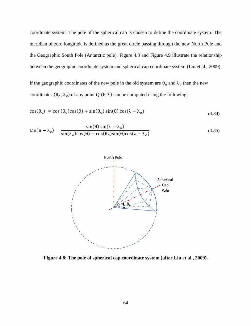
64
coordinate system. The pole of the spherical cap is chosen to define the coordinate system. The
meridian of zero longitude is defined as the great circle passing through the new North Pole and
the Geographic South Pole (Antarctic pole). Figure 4.8 and Figure 4.9 illustrate the relationship
between the geographic coordinate system and spherical cap coordinate system (Liu et al., 2009).
If the geographic coordinates of the new pole in the old system are and then the new
coordinates of any point Q can be computed using the following:
(4.34)
(4.35)
Figure 4.8: The pole of spherical cap coordinate system (after Liu et al., 2009).

65
Figure 4.9: Coordinate transformation between geographic coordinate system and
spherical cap coordinate system (after Liu et al., 2009).
4.6.2.2 Computation of the Associated Legendre Function cosPm
n k
The associated Legendre function can be expressed as follows:
(4.36)
where
(4.37)
and the normalizing factor is approximated using Stirling’s formula (Haines, 1985) by:

66
(4.38)
where
From Equation (4.36) it is shown that
(4.39)
where the second term on the right hand side is set to zero when . In order to calculate the
roots , Equation (4.30) must hold. Using Equation (4.36) and Equation (4.39), the values of
can be solved numerically. The values of
up to for are given in Table
4.1.
Table 4.1: Non-integer degreesmkn for half-angle o = 24
0 1 2 3 4 5
0 0
1 5.234 3.978
2 8.661 8.661 6.918
3 12.675 12.252 11.812 9.711
4 16.256 16.256 15.561 14.829 12.435
5 20.157 19.894 19.626 18.722 17.763 15.118

67
Figure 4.10 illustrates the associated Legendre functions for a spherical cap of half-
angle , for , . It is clear that the functions with “odd” are
zero at the boundary of the cap and the conditions in Equation (4.30) are satisfied.
Figure 4.10: Associated Legendre functions for a spherical cap of half-angle o = 24,
for k = 5, m = 0, 1, … 5
4.6.3 Empirical Orthogonal Functions (EOF)
The vertical resolution of the ionospheric tomographic problem is poor. Therefore, a priori
information is used to form the vertical basis functions that span the entire space in the vertical
direction. This is accomplished using Empirical Orthogonal Function (EOF). EOF analysis is a
powerful tool for data analysis and reduction of data dimensions. These functions are widely
used in meteorology. EOFs are derived from empirical data of the ionospheric electron density,
68
such as the International Reference Ionosphere (IRI) model. Using such functions, the vertical
profiles of electron density are obtained. Given the date, time and location of GPS
measurements, the ionospheric electron density profile can be obtained from the
IRI-2007 model (Bilitza and Reinisch, 2008) and specific EOFs can be tailored for different
geophysical conditions. In this way, the electron density profiles are limited to a certain range of
possible solutions. The electron density profile data matrix ( matrix) can be arranged as:
(4.40)
where is the number of voxels, and N is the number of times series. To obtain the
required EOFs, Singular Value Decomposition (SVD) can be used:
(4.41)
where U and V are orthogonal matrices with columns that span the data and model spaces
respectively, and S is a diagonal matrix:
(4.42)
where the singular values along the diagonal of S are customarily arranged in decreasing order:
··· 0 (4.43)
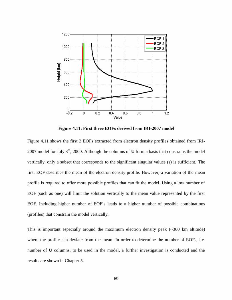
69
Figure 4.11: First three EOFs derived from IRI-2007 model
Figure 4.11 shows the first 3 EOFs extracted from electron density profiles obtained from IRI-
2007 model for July 3rd
, 2000. Although the columns of U form a basis that constrains the model
vertically, only a subset that corresponds to the significant singular values (s) is sufficient. The
first EOF describes the mean of the electron density profile. However, a variation of the mean
profile is required to offer more possible profiles that can fit the model. Using a low number of
EOF (such as one) will limit the solution vertically to the mean value represented by the first
EOF. Including higher number of EOF’s leads to a higher number of possible combinations
(profiles) that constrain the model vertically.
This is important especially around the maximum electron density peak (~300 km altitude)
where the profile can deviate from the mean. In order to determine the number of EOFs, i.e.
number of U columns, to be used in the model, a further investigation is conducted and the
results are shown in Chapter 5.

70
Combining spherical cap harmonic functions and the EOFs, the electron density distribution
can be expressed as follows:
(4.44)
where represents the empirical orthogonal function, is the order of EOFs, and
are the tomography model coefficients that characterize the field of the ionosphere and the
unknowns to be estimated in the model. Based on Equation (4.44), the number of unknowns is:
(4.45)
Equation (4.44) is expressed in a matrix form as:
(4.46)
where contains the basis functions generated using EOFs and SCH expansion, and contains
the tomography model coefficients. Substituting Equation (4.46) in Equation (4.24), the
ionospheric tomography problem can be expressed as follows:
(4.47)
where
(4.48)
71
4.7 Weighted Least Squares
In Equation(4.47), the change in STEC is expressed as a linear system of the form:
(4.49)
where is defined in Equation (4.48), are the change in the observed STECs, and is the
vector of the tomography model coefficients to be estimated. To solve this system of equations,
the method of least squares is used. This method finds the vector which minimizes the sum of
the squares of the errors made in solving every equation. In other words, the least squares
method minimizes the 2-norm of the residuals. The residual is defined as the difference between
the observation and its expected value. In a vector form, the residual vector is defined by:
(4.50)
However, any a priori information about the accuracy of the observation must be taken into
account when solving Equation (4.49). As a result, the weighted least squares solution satisfies
the following (Bjõrck, 1996):
min (4.51)
and the weighted least squares solution can be expressed as follows:
given
(4.52)
where is the initial parameter estimates, is the a priori variance, and is the
measurement variance-covariance matrix. The variance-covariance matrix of the estimated
parameters is given by
(4.53)
where is the a postoriori variance of unit weight which is computed by
72
(4.54)
where is the number of observations and is the number of unknowns .
4.8 Generalized Tikhonov Regularization
The design matrix in Equation (4.48) is nearly singular (large condition number with respect to
singular values). It is difficult to invert it without round-off errors affecting the solution and even
causing it to converge to the wrong solution. Therefore, ionospheric tomography is part of the
family of inverse problems. The ionospheric tomography inverse problem is often ill-posed,
which is characterized by instability, non-uniqueness and even non-existence of the solution.
Therefore, ordinary inversion techniques (i.e. ordinary least squares) are not efficient and special
inversion techniques must be considered in ionospheric tomography.
Many methods have been proposed for regularizing such a problem in order to achieve
reasonable estimates. Generalized Tikhonov regularization is one of the most common methods
for regularization that satisfies the following (Mead, 2007).
min
(4.55)
where and are the inverse of the variance-covariance matrix of the observations and the
initial parameter estimates , respectively. The regularization parameter ≥ 0 controls the
weight given to the norm of , relative to the minimization of the residual norm. The
parameter can be determined using a technique explained in Section 4.8.1. Setting the
following
(4.56)

73
Equation (4.55) is transformed to a simpler form and the minimization problem is replaced with:
(4.57)
Equation (4.57) can be written as
(4.58)
which can be solved by the method of normal equations, i.e.,
(4.59)
Equation (4.59) simplifies to
(4.60)
and the solution of the minimization problem of Equation (4.57) can be written as
(4.61)
Substituting Equation (4.56) in Equation (4.61), the generalized Tikhonov solution of Equation
(4.55) can be expressed as follows:
(4.62)
and the variance-covariance matrix is given by:
(4.63)
where is the a postoriori variance of unit weight which is computed by
(4.64)
where is the number of observation and is the number of unknowns.

74
4.8.1 Regularization Parameter Selection
The choice of regularization parameter is a key element of any Tikhonov regularized solution.
If is chosen to be too small, the solution will be dominated by noise. If is chosen too large,
the solution will be too smooth and major features of the distribution will not appear in the
solution. The method of L-curve is the most common method for selecting a regularization
parameter . The L-curve is an L-shaped plot of optimal values of versus
on a log-log scale. The regularization parameter is selected so that it gives the
solution closest to the L-curve corner (Aster et al., 2012). Figure 4.12 shows the generic form of
the L-curve. Once the optimum value is computed, the generalized Tikhonov solution and its
variance-covariance matrix are computed using Equation (4.62) and Equation (4.63),
respectively.
Figure 4.12: The L-curve
75
4.9 Advantages of Ionospheric Tomography
Three-dimensional ionospheric tomography has many advantages. Compared to two-dimensional
imaging, ionospheric tomography has the capability to model the electron density with multiple
layers which is an improvement over two-dimensional imaging. This is beneficial since it
provides more fundamental information about the ionosphere and many ionospheric parameters
can be derived from the electron density profile such as maximum peak value and height.
Therefore ionospheric tomography is regarded as an important cost effective tool to monitor and
study the ionosphere. (Meggs et al., 2004) and (Meggs and Mitchell, 2006) investigated the
benefits gained by using three-dimensional tomography over the two-dimensional imaging over
a wide geographical area. Results showed that both algorithms gave comparable results during
the nighttime; however, the uncertainty in TEC determination during the daytime using two-
dimensional imaging were up to three times greater than those produced by the three-
dimensional ionospheric tomography.
4.10 Applications of Ionospheric Tomography
Ionospheric tomography is useful for many applications. One application is frequency selection
for HF radio communication. Signals at High Frequency (HF) are reflected back to the Earth.
The electron density defines the refractive path of the signals, which is important for radio
frequency selection. It helps in determining the Maximum Usable Frequency (MUF) and Lowest
Usable Frequency (LUF) which are important parameters for a successful communication.
Ionospheric tomography can be used to recover information about the electron density
distribution and aid in planning the MUF and LUF for HF radio communication. (Rogers et al.,
2001) showed that ionospheric tomography can be used to help scheduling HF communications.
76
Range errors due to the ionosphere are the main error source in GPS positioning. Many real-time
mapping systems such as WAAS monitor the ionosphere continuously and provide correction to
single-frequency GPS users to compensate for such range errors. The accuracy of the ionospheric
model determines the position accuracy of single-frequency users. As stated earlier, (Meggs et
al., 2004) and (Meggs and Mitchell, 2006) showed that three-dimensional imaging provides
more accurate TEC maps than those produced by two-dimensional imaging. Therefore,
ionospheric tomography has potential application in deriving ionospheric corrections for wide
area networks.

77
Chapter Five: Ionospheric Tomography Modelling – Simulation
5.1 Introduction
A new ionospheric tomographic technique has been developed and presented in Chapter 4. To
demonstrate the feasibility of the technique, a number of simulations using the IRI model are
performed. Simulations of different ionospheric conditions are used to investigate the capability
of the technique to recover different ionospheric parameters such as electron density, TEC, and
electron density peak value. The conditions are divided into two categories: 1) nominal
ionospheric conditions, and 2) storm conditions. The first category represents typical ionospheric
conditions during different phases of the solar cycle. Three periods of the solar cycle are chosen:
sunspot minimum, maximum and moderate. The second category represents challenging storm
conditions such as a storm enhanced density (SED) event. In this chapter, the feasibility and
performance of the technique under these conditions are demonstrated and analyzed, via
simulation, and a quantitative comparison of the results is conducted and discussed. The outcome
of the analysis determines the most appropriate combination of and Q in Equation (4.44)
for the Canadian polar region, where these values are adopted for the processing of real data in
the Chapter 6.
5.2 Tomographic Modelling of Canadian Polar Region
The region of interest in this thesis is the polar cap, due to its importance and effect on radio
propagation and communication especially during solar maximum. The polar cap region is
lacking spatial resolution of TEC measurements due to the orbit limitations of spaced-based
measurements and sparse networks providing such measurements. To overcome these
limitations, the Canadian High Arctic Ionospheric Network (CHAIN) was designed and took
advantage of Canada's most accessible landmass in the high arctic regions (Jayachandran et al.,

78
2009). The network consists of 10 (eight within the polar cap region) high data-rate GPS
ionospheric scintillation and TEC monitors and six Canadian Advanced Digital Ionosondes
(CADI). Having access to such data, and applying the new Computerized Ionospheric
Tomographic (CIT) technique, a clear understanding of the quality and limitations of the
technique, particularly in high-latitude regions, is achieved. The importance of the
implementation of the new tomographic technique allows determination of various ionospheric
parameters. For example the peak height of electron density is used in monitoring and predicting
HF communication capabilities for aircraft polar routes. Imaging the three-dimensional extent of
ionospheric structures allows identification of gradients associated with development of
ionospheric scintillations. Velocities of such polar cap patches can be estimated and evolution of
scintillation regions predicted.
5.3 Simulated Data Description
Simulations are based on availability of real data in high-latitude regions. Ten GPS reference
stations from the CHAIN Network are used and twenty-six International Global Navigation
Satellite System (GNSS) Service (IGS) stations are selected to form the network over the
Canadian polar region. The coordinates of the network stations used are listed in Table 5.1 and
their geographic distribution is illustrated in Figure 5.1. All sites are equipped with dual-
frequency GPS receivers. This allows the derivation of STEC at each site using the procedure
presented in Chapter 4. Once the coordinates of the ground receivers and the GPS satellites are
known, electron density profiles can be recovered and TEC maps can be computed using the
proposed CIT technique.
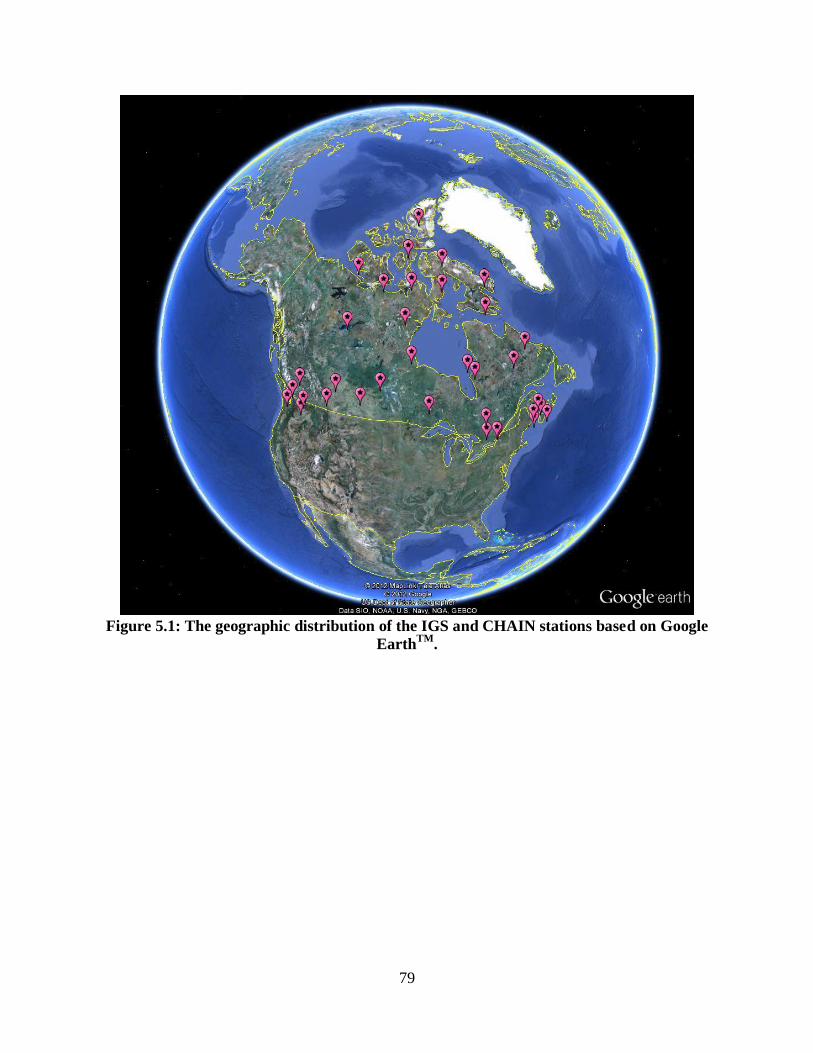
79
Figure 5.1: The geographic distribution of the IGS and CHAIN stations based on Google
EarthTM
.
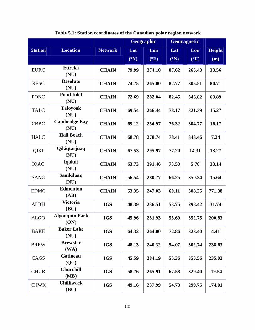
80
Table 5.1: Station coordinates of the Canadian polar region network
Station Location Network
Geographic Geomagnetic
Height
(m)
Lat
(°N)
Lon
(°E)
Lat
(°N)
Lon
(°E)
EURC Eureka
(NU) CHAIN 79.99 274.10 87.62 265.43 33.56
RESC Resolute
(NU) CHAIN 74.75 265.00 82.77 305.51 80.71
PONC Pond Inlet
(NU) CHAIN 72.69 282.04 82.45 346.82 63.89
TALC Taloyoak
(NU) CHAIN 69.54 266.44 78.17 321.39 15.27
CBBC Cambridge Bay
(NU) CHAIN 69.12 254.97 76.32 304.77 16.17
HALC Hall Beach
(NU) CHAIN 68.78 278.74 78.41 343.46 7.24
QIKI Qikiqtarjuaq
(NU) CHAIN 67.53 295.97 77.20 14.31 13.27
IQAC Iqaluit
(NU) CHAIN 63.73 291.46 73.53 5.78 23.14
SANC Sanikiluaq
(NU) CHAIN 56.54 280.77 66.25 350.34 15.64
EDMC Edmonton
(AB) CHAIN 53.35 247.03 60.11 308.25 771.38
ALBH Victoria
(BC) IGS 48.39 236.51 53.75 298.42 31.74
ALGO Algonquin Park
(ON) IGS 45.96 281.93 55.69 352.75 200.83
BAKE Baker Lake
(NU) IGS 64.32 264.00 72.86 323.40 4.41
BREW Brewster
(WA) IGS 48.13 240.32 54.07 302.74 238.63
CAGS Gatineau
(QC) IGS 45.59 284.19 55.36 355.56 235.02
CHUR Churchill
(MB) IGS 58.76 265.91 67.58 329.40 -19.54
CHWK Chilliwack
(BC) IGS 49.16 237.99 54.73 299.75 174.01
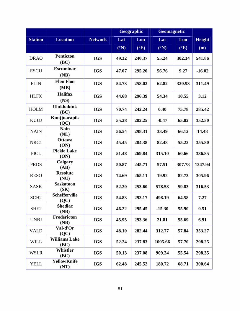
81
Station Location Network
Geographic Geomagnetic
Height
(m)
Lat
(°N)
Lon
(°E)
Lat
(°N)
Lon
(°E)
DRAO Penticton
(BC) IGS 49.32 240.37 55.24 302.34 541.86
ESCU Escuminac
(NB) IGS 47.07 295.20 56.76 9.27 -16.02
FLIN Flon Flon
(MB) IGS 54.73 258.02 62.82 320.93 311.49
HLFX Halifax
(NS) IGS 44.68 296.39 54.34 10.55 3.12
HOLM Ulukhaktok
(BC) IGS 70.74 242.24 0.40 75.78 285.42
KUUJ Kuujjuarapik
(QC) IGS 55.28 282.25 -0.47 65.02 352.50
NAIN Nain
(NL) IGS 56.54 298.31 33.49 66.12 14.48
NRC1 Ottawa
(ON) IGS 45.45 284.38 82.48 55.22 355.80
PICL Pickle Lake
(ON) IGS 51.48 269.84 315.10 60.66 336.85
PRDS Calgary
(AB) IGS 50.87 245.71 57.51 307.78 1247.94
RESO Resolute
(NU) IGS 74.69 265.11 19.92 82.73 305.96
SASK Saskatoon
(SK) IGS 52.20 253.60 578.58 59.83 316.53
SCH2 Schefferville
(QC) IGS 54.83 293.17 498.19 64.58 7.27
SHE2 Shediac
(NB) IGS 46.22 295.45 -15.30 55.90 9.51
UNBJ Fredericton
(NB) IGS 45.95 293.36 21.81 55.69 6.91
VALD Val-d'Or
(QC) IGS 48.10 282.44 312.77 57.84 353.27
WILL Williams Lake
(BC) IGS 52.24 237.83 1095.66 57.70 298.25
WSLR Whistler
(BC) IGS 50.13 237.08 909.24 55.54 298.35
YELL YellowKnife
(NT) IGS 62.48 245.52 180.72 68.71 300.64
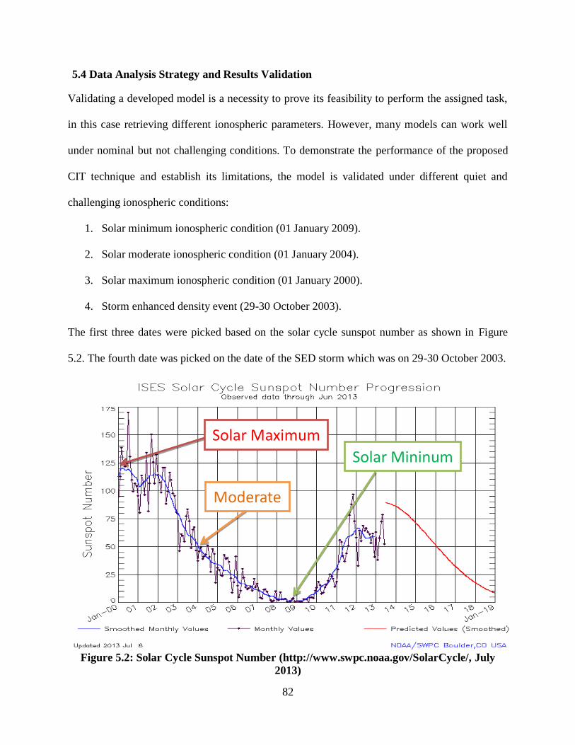
82
5.4 Data Analysis Strategy and Results Validation
Validating a developed model is a necessity to prove its feasibility to perform the assigned task,
in this case retrieving different ionospheric parameters. However, many models can work well
under nominal but not challenging conditions. To demonstrate the performance of the proposed
CIT technique and establish its limitations, the model is validated under different quiet and
challenging ionospheric conditions:
1. Solar minimum ionospheric condition (01 January 2009).
2. Solar moderate ionospheric condition (01 January 2004).
3. Solar maximum ionospheric condition (01 January 2000).
4. Storm enhanced density event (29-30 October 2003).
The first three dates were picked based on the solar cycle sunspot number as shown in Figure
5.2. The fourth date was picked on the date of the SED storm which was on 29-30 October 2003.
Figure 5.2: Solar Cycle Sunspot Number (http://www.swpc.noaa.gov/SolarCycle/, July
2013)
Solar Maximum
Moderate
Solar Mininum
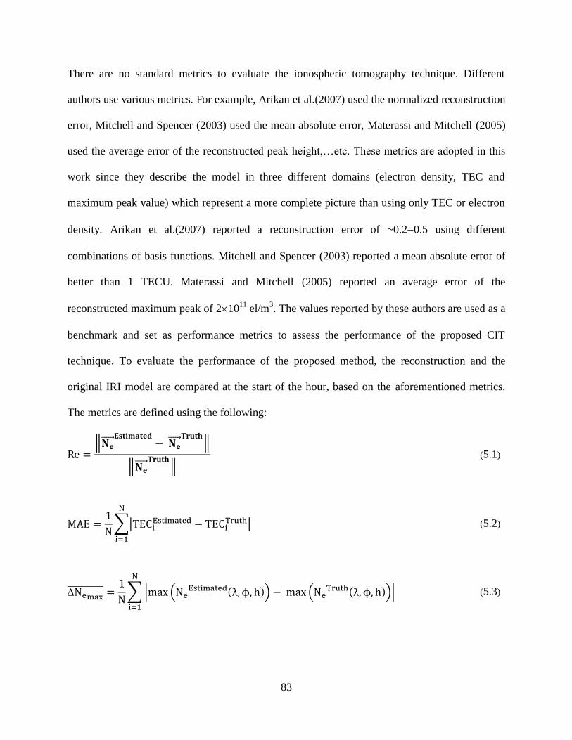
83
There are no standard metrics to evaluate the ionospheric tomography technique. Different
authors use various metrics. For example, Arikan et al.(2007) used the normalized reconstruction
error, Mitchell and Spencer (2003) used the mean absolute error, Materassi and Mitchell (2005)
used the average error of the reconstructed peak height,…etc. These metrics are adopted in this
work since they describe the model in three different domains (electron density, TEC and
maximum peak value) which represent a more complete picture than using only TEC or electron
density. Arikan et al.(2007) reported a reconstruction error of ~0.20.5 using different
combinations of basis functions. Mitchell and Spencer (2003) reported a mean absolute error of
better than 1 TECU. Materassi and Mitchell (2005) reported an average error of the
reconstructed maximum peak of 2 1011
el/m3. The values reported by these authors are used as a
benchmark and set as performance metrics to assess the performance of the proposed CIT
technique. To evaluate the performance of the proposed method, the reconstruction and the
original IRI model are compared at the start of the hour, based on the aforementioned metrics.
The metrics are defined using the following:
(5.1)
(5.2)
(5.3)
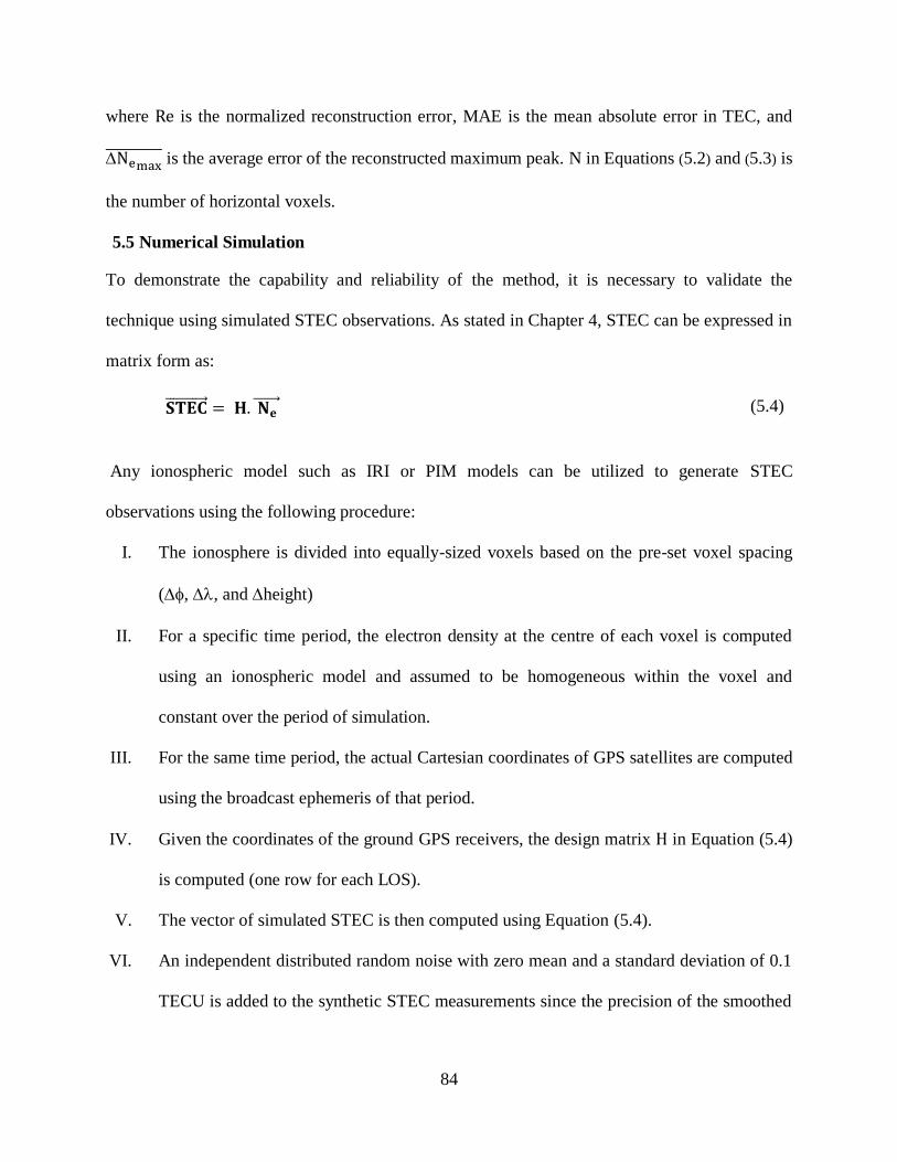
84
where is the normalized reconstruction error, MAE is the mean absolute error in TEC, and
is the average error of the reconstructed maximum peak. N in Equations (5.2) and (5.3) is
the number of horizontal voxels.
5.5 Numerical Simulation
To demonstrate the capability and reliability of the method, it is necessary to validate the
technique using simulated STEC observations. As stated in Chapter 4, STEC can be expressed in
matrix form as:
(5.4)
Any ionospheric model such as IRI or PIM models can be utilized to generate STEC
observations using the following procedure:
I. The ionosphere is divided into equally-sized voxels based on the pre-set voxel spacing
( , , and height)
II. For a specific time period, the electron density at the centre of each voxel is computed
using an ionospheric model and assumed to be homogeneous within the voxel and
constant over the period of simulation.
III. For the same time period, the actual Cartesian coordinates of GPS satellites are computed
using the broadcast ephemeris of that period.
IV. Given the coordinates of the ground GPS receivers, the design matrix in Equation (5.4)
is computed (one row for each LOS).
V. The vector of simulated STEC is then computed using Equation (5.4).
VI. An independent distributed random noise with zero mean and a standard deviation of 0.1
TECU is added to the synthetic STEC measurements since the precision of the smoothed
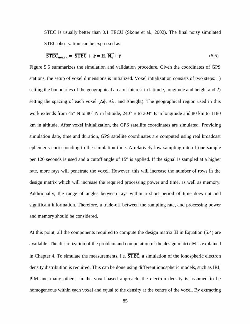
85
STEC is usually better than 0.1 TECU (Skone et al., 2002). The final noisy simulated
STEC observation can be expressed as:
(5.5)
Figure 5.5 summarizes the simulation and validation procedure. Given the coordinates of GPS
stations, the setup of voxel dimensions is initialized. Voxel intialization consists of two steps: 1)
setting the boundaries of the geographical area of interest in latitude, longitude and height and 2)
setting the spacing of each voxel ( , , and height). The geographical region used in this
work extends from 45 N to 80 N in latitude, 240 E to 304 E in longitude and 80 km to 1180
km in altitude. After voxel initialization, the GPS satellite coordinates are simulated. Providing
simulation date, time and duration, GPS satellite coordinates are computed using real broadcast
ephemeris corresponding to the simulation time. A relatively low sampling rate of one sample
per 120 seconds is used and a cutoff angle of 15 is applied. If the signal is sampled at a higher
rate, more rays will penetrate the voxel. However, this will increase the number of rows in the
design matrix which will increase the required processing power and time, as well as memory.
Additionally, the range of angles between rays within a short period of time does not add
significant information. Therefore, a trade-off between the sampling rate, and processing power
and memory should be considered.
At this point, all the components required to compute the design matrix H in Equation (5.4) are
available. The discretization of the problem and computation of the design matrix H is explained
in Chapter 4. To simulate the measurements, i.e. , a simulation of the ionospheric electron
density distribution is required. This can be done using different ionospheric models, such as IRI,
PIM and many others. In the voxel-based approach, the electron density is assumed to be
homogeneous within each voxel and equal to the density at the centre of the voxel. By extracting
86
the centre coordinates of each voxel and passing them to the ionosphere simulator along with the
simulation date and time used to simulate GPS satellite coordinates, the ionosphere is simulated
and the truth electron density profile
is generated. Using Equation (5.4) noise free
synthetic is computed.
To make the simulation more realistic, white Gaussian noise with a standard deviation of 0.1
TECU is added to the synthetic STEC. The design matrix H and the measurements vector
are differenced with respect to the reference measurement to eliminate the satellite and receiver
inter-frequency biases. The outcome of the differencing operation H and are passed to
the ionospheric tomography engine. However, to apply the proposed CIT technique, the
spherical cap harmonics parameters and the empirical orthogonal functions are required.
Empirical orthogonal functions are computed using the procedure provided in Chapter 4. The
spherical cap harmonics are computed after setting the spherical cap pole and half-angle . The
pole is set at the centre of the area of interest, i.e. 62.5 N and 272 E and the half-angle is set
equal to half of the latitude span plus a small number to assure the coverage of the longitude
span. It is found that the half-angle required to cover the area is 27.5. Figure 5.3 shows the
boundary of the area of interest (green) and the spherical cap boundary (red) required to cover
such an area.

87
Figure 5.3: Spherical cap boundary (red) and voxel footprints (green)
Setting the number of empirical orthogonal functions (Q) and the maximum order of spherical
cap harmonics ( ), the basis functions expressed in a matrix form are computed. Using the
design matrix H, the measurements vector and the basis functions matrix B, the
tomography model coefficients of Equation (4.44) are estimated using Generalized Tikhonov
regularization technique. The estimated electron distribution is then computed using the
following:
(5.6)

88
Equations (5.1), (5.2), and (5.3) are used to assess and validate the inversion technique. The
output of the inversion technique is the electron density distribution. TEC is required to compute
the metric MAE. TEC can be computed as shown in Figure 5.4. For simplicity, the ionosphere is
schematically divided into 9 voxels where each voxel is assigned a different electron density
value. Since the voxels’ centres are equally spaced, TEC above a point can be computed
using the trapezoidal rule as:
(5.7)
where the units of and are el/m3 and m, respectively. For example, the TEC above
point is equal to and above is equal to
.
Figure 5.4: Computation of vertical TEC

89
Figure 5.5: Flow chart summarizing the simulation and validation procedure
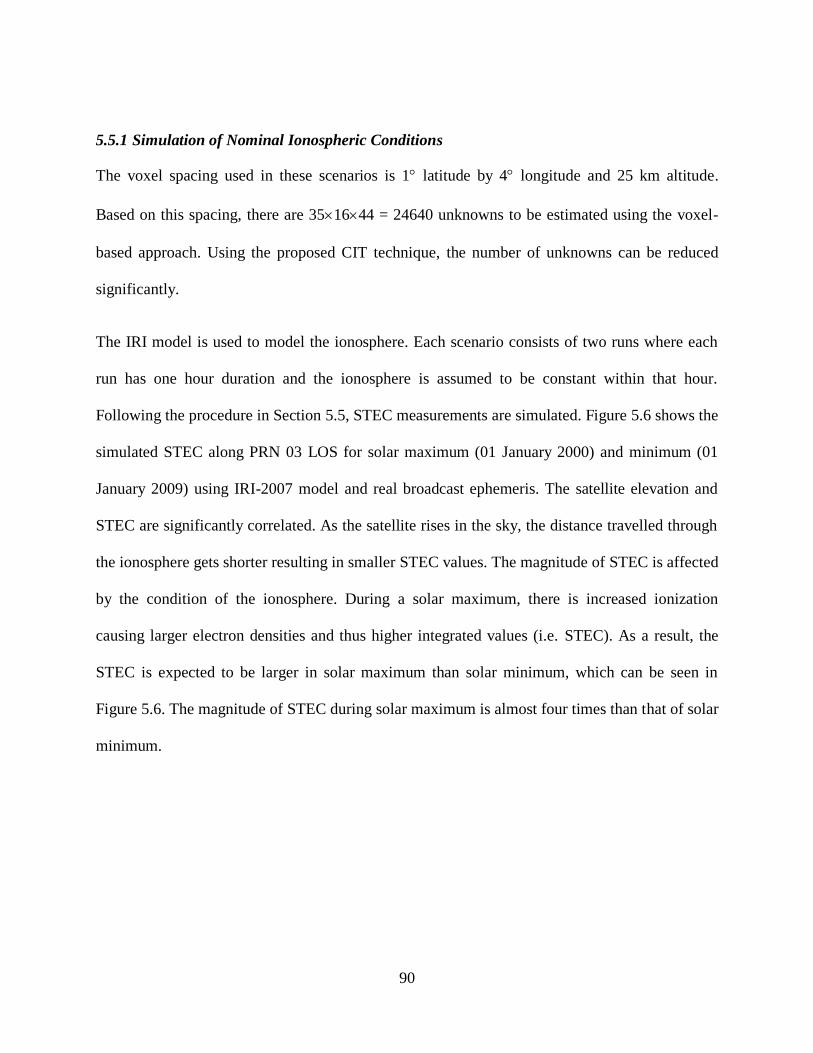
90
5.5.1 Simulation of Nominal Ionospheric Conditions
The voxel spacing used in these scenarios is 1 latitude by 4 longitude and 25 km altitude.
Based on this spacing, there are 35 16 44 = 24640 unknowns to be estimated using the voxel-
based approach. Using the proposed CIT technique, the number of unknowns can be reduced
significantly.
The IRI model is used to model the ionosphere. Each scenario consists of two runs where each
run has one hour duration and the ionosphere is assumed to be constant within that hour.
Following the procedure in Section 5.5, STEC measurements are simulated. Figure 5.6 shows the
simulated STEC along PRN 03 LOS for solar maximum (01 January 2000) and minimum (01
January 2009) using IRI-2007 model and real broadcast ephemeris. The satellite elevation and
STEC are significantly correlated. As the satellite rises in the sky, the distance travelled through
the ionosphere gets shorter resulting in smaller STEC values. The magnitude of STEC is affected
by the condition of the ionosphere. During a solar maximum, there is increased ionization
causing larger electron densities and thus higher integrated values (i.e. STEC). As a result, the
STEC is expected to be larger in solar maximum than solar minimum, which can be seen in
Figure 5.6. The magnitude of STEC during solar maximum is almost four times than that of solar
minimum.

91
Figure 5.6: Simulated STEC along PRN 3 line-of-sight for Churchill site in solar maximum
(top) and solar minimum (bottom)
Figure 5.7 shows the simulated Vertical TEC using IRI model for the three simulated scenarios
over the centre voxel (62.5 N and 272 E) over 24 hours in local time. Two important features
can be extracted from the figure: The diurnal variation and the peak value of the vertical TEC.
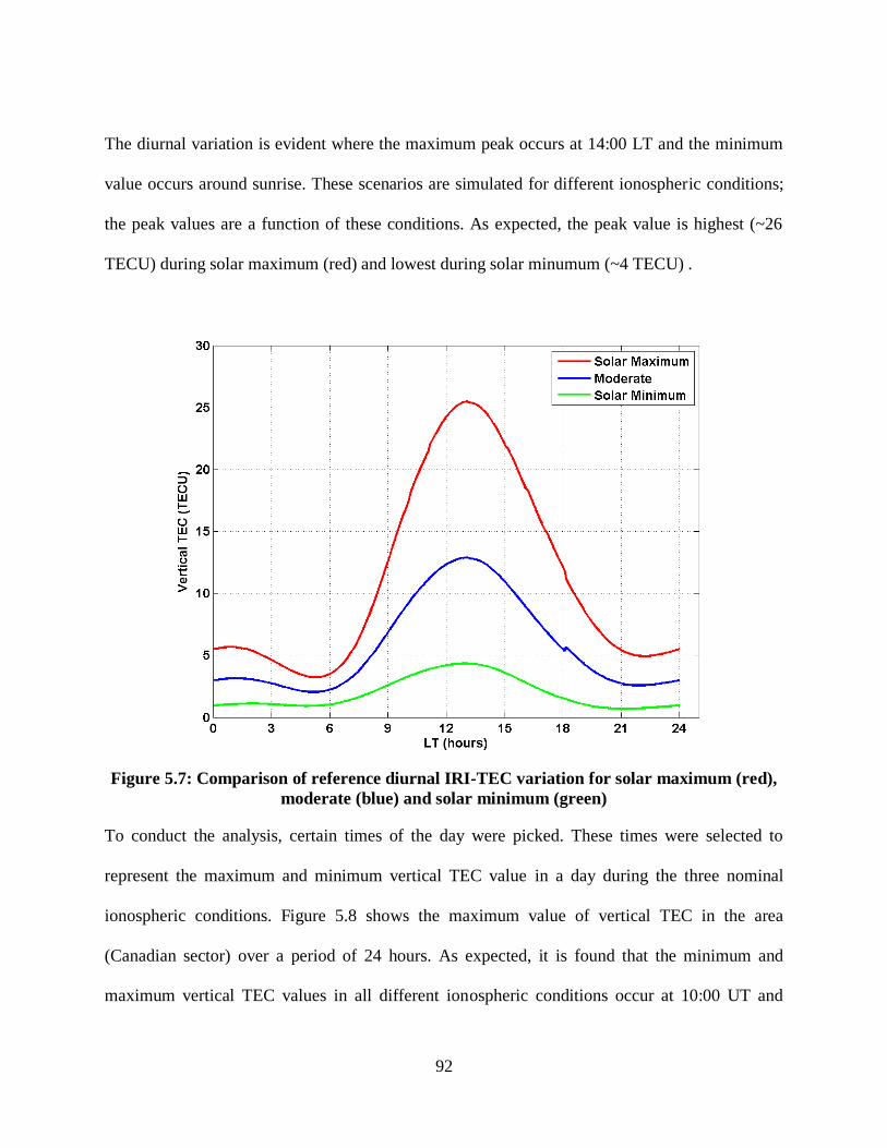
92
The diurnal variation is evident where the maximum peak occurs at 14:00 LT and the minimum
value occurs around sunrise. These scenarios are simulated for different ionospheric conditions;
the peak values are a function of these conditions. As expected, the peak value is highest (~26
TECU) during solar maximum (red) and lowest during solar minumum (~4 TECU) .
Figure 5.7: Comparison of reference diurnal IRI-TEC variation for solar maximum (red),
moderate (blue) and solar minimum (green)
To conduct the analysis, certain times of the day were picked. These times were selected to
represent the maximum and minimum vertical TEC value in a day during the three nominal
ionospheric conditions. Figure 5.8 shows the maximum value of vertical TEC in the area
(Canadian sector) over a period of 24 hours. As expected, it is found that the minimum and
maximum vertical TEC values in all different ionospheric conditions occur at 10:00 UT and

93
21:00 UT, respectively. Therefore, the investigation and the analysis of results are conducted for
these specific hours.
Figure 5.8: Comparison of reference diurnal maximum IRI-TEC variation for solar
maximum (red), moderate (blue) and solar minimum (green) in the Canadian sector
Vertical TEC maps computed from simulated electron density profiles are shown in Figure 5.9.
Different levels of TEC values are evident during different solar cycle periods. While low TEC
values (0.75 – 7 TECU) are common for all solar cycle periods at approximately 10:00 UT,
higher values are dominant over much of Canada at 21:00 UT. The ionosphere’s dependence on
solar activity cycle is observed when comparing the vertical TEC values between 21:00 UT
during solar minimum and 10:00 UT during solar maximum. The minimum values of vertical
TEC (at 10:00 UT) during solar maximum are close to the maximum values of the day (at 21:00
UT) during solar minimum, which emphasizes the high correlation of vertical TEC with the solar
cycle.
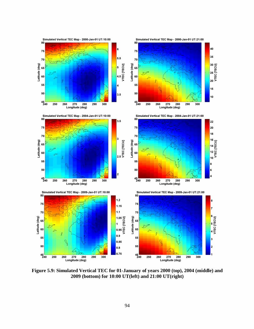
94
Figure 5.9: Simulated Vertical TEC for 01-January of years 2000 (top), 2004 (middle) and
2009 (bottom) for 10:00 UT(left) and 21:00 UT(right)

95
5.5.2 Simulation of Storm Ionospheric Conditions
The Storm Enhanced Density (SED) phenomenon can occur over North America. The SED is
characterized by a plume of enhanced electron density evolving and extending to higher latitudes
(Coster and Skone, 2009). The plume is associated with large vertical TEC gradients causing a
sharp drop of TEC values at the edges. Such localized ionospheric events and TEC gradients
cause large differential ionospheric range errors affecting Differential GPS (DGPS) and Wide
Area Augmentation System (WAAS) users especially near the SED plume where positioning
errors can exceed more than 20m (Coster and Skone, 2009).
Modelling SED in three dimensions is challenging and has not been added to available
ionospheric models, such as IRI. Therefore, the simulation of this event was done with the
assistance of external data. The electron density distribution during 29-30 October 2003 storm
was estimated using IDA3D model (Bust et al., 2004). The electron density profile for 21:00 UT
was provided along 240 E longitude using 5 latitude spacing. A voxel spacing of 5 in latitude,
5 in longitude and 25km in altitude is used for the SED simulation. For simulation purposes,
these profiles are shifted to the middle of the area of interest at 266.5 E. IRI model is also used
as background and the electron density is simulated at the centre of the remaining voxels to
compensate for the missing electron density profiles. This simple approach initially results in
unrealistic electron density profiles since there are only high electron density values along 266.5
E longitude which is ~30 times greater than those simulated by IRI. Therefore, a weighted
averaging of the IDA3D and IRI electron density profiles is used to simulate large westward and
northward gradients at the edges of the plume. The simulation of the electron density profile
along 266.5 E longitude and the vertical TEC map are shown in Figure 5.10.

96
Figure 5.10: Simulated electron density profile (left) and vertical TEC map (right) of a
storm enhanced density
Table 5.2: Simulation settings
Nominal conditions Storm conditions
(SED)
Region boundaries
= 45 N 80 N
= 240 E 304 E
height = 80 km 1180 km
Voxel spacing
( height) 1 4 25km 5 5 25km
Ionosphere
simulator IRI – 2007
External source
(IDA3D)
+
IRI-2007
Simulation
date and year
Solar maximum (01 Jan 2000)
Solar moderate (01 Jan 2004)
Solar minimum (01 Jan 2009)
SED (30 Oct 2003)
Simulation
time of day 10:00 UT and 21:00 UT 21:00 UT
Simulation
duration 60 minutes
Data sampling rate Sample per 120 seconds
SCH pole 62.5 N and 272 E
SCH half-angle 27.5

97
5.6 Determination of SCH and Number of EOF
The degree of Spherical cap harmonics (Kmax) and the number of empirical orthogonal functions
(Q) control the number of unknowns to be estimated. Using lower Kmax and Q leads to lower
number of unknowns. Choosing high degree and number of EOFs generally results in a better
representation (higher resolution) of the electron density profile, but this makes the design matrix
singular and severely ill-conditioned which can make the problem susceptible to noise and small
errors affecting the solution - even causing it to converge to the wrong solution. Therefore,
determining the appropriate degree of spherical cap harmonics (Kmax) and the number of
empirical orthogonal functions (Q) is important in this model.
As will be shown later, high values of Q and Kmax result in better fitting. However, the condition
number of the design matrix will be very high affecting the accuracy of the inversion
significantly. Therefore, a trade-off between model accuracy and ability to invert the problem
must be considered. The determination process consists of two parts: 1) evaluation of the system
model representing the electron density, i.e. SCH and EOF, and 2) evaluation of the
measurement model and the proposed CIT technique to reconstruct the electron density. In the
first part, the lowest possible values of and Q are determined and these values are used to
evaluate the measurement model.
Since the ionospheric tomography problem is a severely ill-conditioned problem, the level of
noise and the observation geometry play a major role in the performance of the proposed
technique. Therefore, the initial procedure to determine the optimized and Q values is
based on how well the model can describe the electron density distribution, i.e. Equation (4.44).
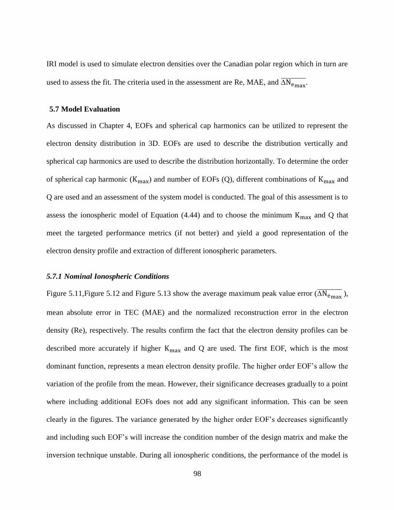
98
IRI model is used to simulate electron densities over the Canadian polar region which in turn are
used to assess the fit. The criteria used in the assessment are Re, MAE, and .
5.7 Model Evaluation
As discussed in Chapter 4, EOFs and spherical cap harmonics can be utilized to represent the
electron density distribution in 3D. EOFs are used to describe the distribution vertically and
spherical cap harmonics are used to describe the distribution horizontally. To determine the order
of spherical cap harmonic ( ) and number of EOFs (Q), different combinations of and
Q are used and an assessment of the system model is conducted. The goal of this assessment is to
assess the ionospheric model of Equation (4.44) and to choose the minimum and Q that
meet the targeted performance metrics (if not better) and yield a good representation of the
electron density profile and extraction of different ionospheric parameters.
5.7.1 Nominal Ionospheric Conditions
Figure 5.11,Figure 5.12 and Figure 5.13 show the average maximum peak value error ( ),
mean absolute error in TEC (MAE) and the normalized reconstruction error in the electron
density (Re), respectively. The results confirm the fact that the electron density profiles can be
described more accurately if higher and Q are used. The first EOF, which is the most
dominant function, represents a mean electron density profile. The higher order EOF’s allow the
variation of the profile from the mean. However, their significance decreases gradually to a point
where including additional EOFs does not add any significant information. This can be seen
clearly in the figures. The variance generated by the higher order EOF’s decreases significantly
and including such EOF’s will increase the condition number of the design matrix and make the
inversion technique unstable. During all ionospheric conditions, the performance of the model is

99
poor when using Q = 1 or 2. The performance improves drastically if Q = 3 or higher is used.
This is expected since using higher degree of EOF’s allows the model to represent the profile
accurately especially around the maximum peak height (~300 km altitude) as explained earlier in
Chapter 4. As a result, the minimum value of Q that should be used in this model should be
higher than or equal to three.
EOF’s are used as the basis function describing the profiles vertically. To be able to represent the
profile horizontally, spherical cap harmonics are used. For cases where Q = 3, results show that
the minimum at which the results are improved significantly is equal to three. As a result,
the minimum optimum values of and Q over the Canadian polar region chosen for this
work are chosen to be 3 and 3, respectively.

100
Figure 5.11: Average maximum peak value error for 01-January of years 2000
(top), 2004 (middle) and 2009 (bottom) for UT 10:00 (left) and UT 21:00 (right)
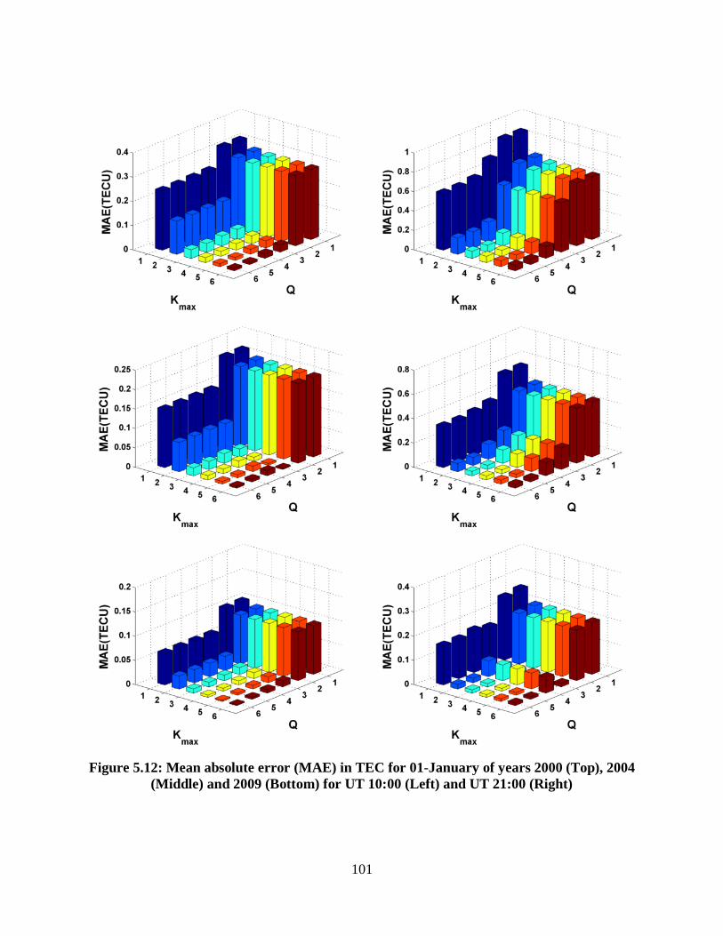
101
Figure 5.12: Mean absolute error (MAE) in TEC for 01-January of years 2000 (Top), 2004
(Middle) and 2009 (Bottom) for UT 10:00 (Left) and UT 21:00 (Right)
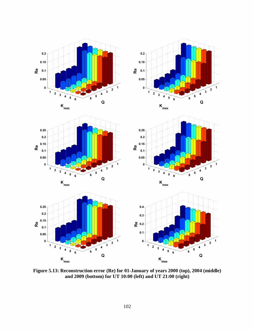
102
Figure 5.13: Reconstruction error (Re) for 01-January of years 2000 (top), 2004 (middle)
and 2009 (bottom) for UT 10:00 (left) and UT 21:00 (right)

103
In the previous step, the best minimum and Q values are determined through evaluating the
model fit and how well it can represent the electron density profile. The next step is to test the
performance of the proposed CIT technique using these values. Table 5.3 summarizes the results
of the inversion for the three nominal ionospheric conditions at 10:00 and 21:00 UT. Results
show high correlation between the ionspheric conditions and the different error metrics. As the
solar activity decreases from maximum to minimum, the errors decrease. This is evident in the
average maximum electron density peak where the error is lower for solar minimum
than solar maximum. The same applies to the errors for local day (21:00 UT or 14:00 LT) versus
local night (10:00 UT or 03:00 LT). Re and MAE in TEC behave similarly for day versus night.
However, it is observed that the errors during 2004 (moderate case) are higher than during solar
maximum for MAE and Re.
Table 5.3: Assessment of the model using Kmax = 3 and Q = 3
10:00 UT 21:00 UT
Re MAE
(TECU)
1011
el/m3
Re MAE
(TECU)
1011
el/m3
2000 0.12 0.07 0.31 0.22 0.17 0.91
2004 0.18 0.13 0.16 0.27 0.18 0.73
2009 0.11 0.09 0.10 0.19 0.14 0.20
Since the three cases are similar, the results for 21:00 UT are presented as an example to
demonstrate the capability of the proposed technique for estimating different ionospheric
parameters over the Canadian polar region. Figure 5.14 shows the estimated vertical TEC map
and the associated errors in the estimation. It can be seen that the technique has produced a very
accurate representation of the vertical TEC and the gradients associated with it. The

104
reconstructed maps show underestimation of TEC in some regions and overestimation in other
regions. This is due to the use of a limited number of empirical orthogonal functions and low
degree of spherical cap harmonics. However, a higher degree and number of orthogonal function
will lead to a higher condition number making the design matrix sensitive to small errors
resulting in a worse solution.
The proposed CIT technique estimates the model coefficients rather than the electron density
profiles. The estimated coefficients are then used in Equation (4.46) to describe the electron
density distribution. Figure 5.15 shows an example of the reconstructed electron density profile
along 270 E longitude using the estimated coefficients. It can be observed that most of the
features are well replicated and the image represents the peak height, maximum electron density
and electron density distribution adequately. Re for 01 January 2000, 2004 and 2009 at 21:00 UT
simulations are 0.22, 0.27 and 0.19, respectively, which are within the required values and meet
the targeted performance metrics. The error in the maximum peak height is within 25 km, which
is the thickness of the voxel.

105
Figure 5.14: Estimated vertical TEC maps using simulated IRI STEC (left) and the
difference between the estimated and simulated TEC maps (right) for 01 January 2000
(top), 2004 (middle) and 2009 (bottom) for UT 21:00 (Kmax =3 and Q = 3)

106
Figure 5.15: Simulated (left) and estimated (right) electron density distribution IRI along
270 E longitude for 01 January 2000 (top), 2004 (middle) and 2009 (bottom) for UT 21:00
(Kmax =3 and Q = 3)

107
Residual analysis provides useful information; for example residuals must be checked for
blunders and goodness of fit. Histograms of the residuals for the three ionospheric conditions at
21:00 UT are shown in Figure 5.16. As expected, the residuals are normally distributed, which
confirms the assumption (parameters are normally distributed). The absolute values of the
residuals are less than 0.5 TECU, which indicates statistically a good fit of the solution to the
model given that an independent distributed random noise with standard deviation of 0.1 TECU
is added to the simulated measurements. The root mean square of the residuals is 0.14 TECU
which is higher than the noise standard deviation. This can be explained by the law of
propagation error. As mentioned in Chapter 4, the measurement matrix is differenced to
eliminate the receiver and satellite biases. This operation will increase the noise standard
deviation by a factor of resulting in noise with a standard deviation of
TECU.
As explained earlier, the electron density profiles can be reconstructed using the proposed CIT
technique. Using the reconstructed profiles, the vertical TEC above a given point can be
computed using Equation (4.46) and vertical TEC maps can be generated. Figure 5.17 and Figure
5.18 present the vertical TEC maps on 01 January 2000 for the selected hours. The computed
maps are compared to the simulated vertical TEC maps and the statistics of the errors are
presented in Table 5.4. Slight variation in the accuracy is observed over time. Nevertheless, the
accuracy of the inversion is better than 0.5 TECU.

108
Figure 5.16 Histogram of the residuals for 01 January 2000 (top), 2004 (middle) and 2009
(bottom) for UT 21:00 (Kmax =3 and Q = 3)

109
Figure 5.17:Comparison between simulated (top), estimated (middle) vertical TEC maps
and the error in the estimation (bottom). Results are shown for 01 January 2000 for UT
00:00 (left) and UT 06:00 (right) using Kmax =3 and Q = 3.

110
Figure 5.18 Comparison between simulated (top), estimated (middle) vertical TEC maps
and the error in the estimation (bottom). Results are shown for 01 January 2000 for UT
12:00 (left) and UT 18:00 (right) using Kmax =3 and Q = 3.

111
Table 5.4: Statistics on the vertical TEC error on 01 January 2000.
Hour
(UT)
Min
(TECU)
Max
(TECU)
Mean
(TECU)
RMSE
(TECU)
00:00 -0.13 2.05 0.26 0.19
06:00 -0.53 1.20 0.25 0.31
12:00 -0.85 2.69 -0.35 0.33
18:00 -0.63 1.38 0.35 0.29
5.7.2 Storm Conditions
The model has been tested and challenged in nominal ionospheric conditions during solar
minimum and maximum. To generate additional realistic and quantitative performance measures,
the model is tested under ionospheric storm conditions (in this case SED). An assessment of the
CIT model is conducted under SED challenging conditions.
Using = 3 and Q = 3, the CIT technique produces vertical TEC maps shown in Figure 5.19.
Due to the limitation of the technique, the model is not able to retrieve an accurate representation
of vertical TEC map. The errors in TEC values (MAE = 7.5 TECU) are considerably high,
especially along the plume and its edges. This is due to the fact that the limited number of EOFs
do not fully represent a highly variable ionosphere. IRI model (used to generate the EOF’s) was
derived using long-term mean values of ionospheric measurements. IRI reflects average
approximation of nominal ionosphere conditions which does not include such challenging
conditions as SED. Therefore, even if a higher number of EOFs are used, the results will not
improve and they may be worse due to the fact that the condition number of the design matrix
will be larger causing the model to be more sensitive to errors. This is demonstrated in Table 5.5.
Different Kmax and Q values are used and the statistics of the errors corresponding to the solution

112
using these values are listed. As the number of EOF increases the condition number of the design
matrix increases and as a result the errors become larger.
Figure 5.19: Estimated vertical TEC map (left) and the error in the estimation (right) using
Kmax =3 and Q = 3.
Table 5.5: Error statistics using different Kmax and Q
( Kmax,Q )
Re
MAE
(TECU)
1011
el/m3
Condition
Number
(3,3) 0.55 7.42 1.59 800
(4,4) 0.63 12.28 2.12 8581
(5,5) 0.69 15.50 2.47 73184
Although the proposed CIT technique does not produce accurate images, the solution computed
by the technique minimizes the errors in a least squares sense. To further make use of this
information, the solution can be used as an initial guess and a constraint imposed on the
ionospheric tomography in its original form as in Equation (4.22). This approach forces the
model to be close to the initial guess and refines it to a better solution so that the residuals are
minimized. However, the design matrix (H) is rank-deficient and severely ill-conditioned;
therefore the regularization technique described in Chapter 4 is used to solve the problem. Figure
5.20 shows the refined image using the solution of the proposed CIT as an initial guess. The SED
113
feature is recognisable and the gradients at the edges of the plume are recovered. The errors in
vertical TEC maps are reduced significantly (MAE = 3.7 TECU).
Figure 5.20:Refined vertical TEC map (left) and the error in the estimation (right).
Figure 5.21 shows the estimated electron density using the proposed CIT technique and the
refined estimated electron density achieved by solving the ionospheric tomography model using
the first solution as an initial guess to constrain the model. As explained earlier, CIT using EOF
and SCH does not recover the values of electron density profile accurately. However, this
technique can estimate the peak altitude of maximum electron density adequately. Using the
refinement technique, more features are recovered and better representation of the peak height
and value is achieved. As a result, the reconstruction error of the electron density (Re) is
improved from 0.55 to 0.38.
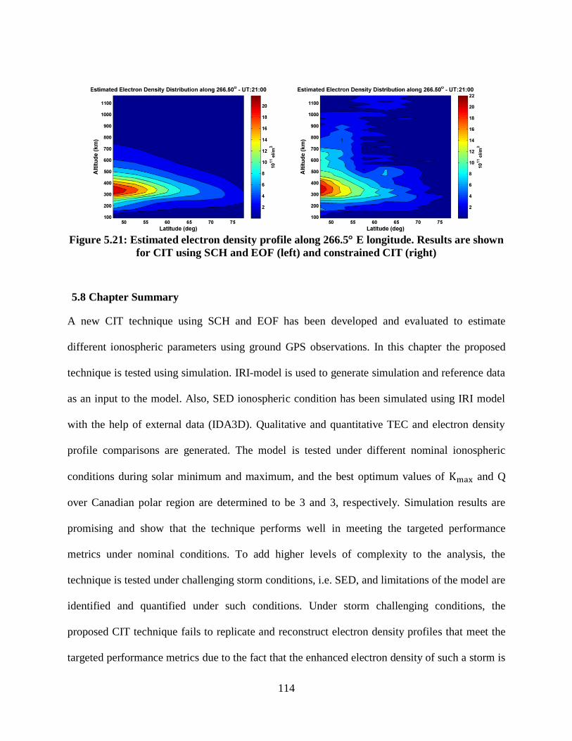
114
Figure 5.21: Estimated electron density profile along 266.5 E longitude. Results are shown
for CIT using SCH and EOF (left) and constrained CIT (right)
5.8 Chapter Summary
A new CIT technique using SCH and EOF has been developed and evaluated to estimate
different ionospheric parameters using ground GPS observations. In this chapter the proposed
technique is tested using simulation. IRI-model is used to generate simulation and reference data
as an input to the model. Also, SED ionospheric condition has been simulated using IRI model
with the help of external data (IDA3D). Qualitative and quantitative TEC and electron density
profile comparisons are generated. The model is tested under different nominal ionospheric
conditions during solar minimum and maximum, and the best optimum values of and Q
over Canadian polar region are determined to be 3 and 3, respectively. Simulation results are
promising and show that the technique performs well in meeting the targeted performance
metrics under nominal conditions. To add higher levels of complexity to the analysis, the
technique is tested under challenging storm conditions, i.e. SED, and limitations of the model are
identified and quantified under such conditions. Under storm challenging conditions, the
proposed CIT technique fails to replicate and reconstruct electron density profiles that meet the
targeted performance metrics due to the fact that the enhanced electron density of such a storm is

115
not modeled in the background ionosphere from which the EOF are derived. Therefore, the basis
functions (EOF) will not be able to model the electron density profile vertically. An approach is
proposed to better estimate the electron density distribution, where the solution of the proposed
CIT technique is used to impose a constraint on the ionospheric tomography in its original form.
However, this approach requires high computational load and memory and inverting the problem
might be challenging, especially if a higher resolution, i.e. higher number of unknowns, is
required.
116
Chapter Six: Ionospheric Tomography Modelling – Real Data
6.1 Introduction
As determined in Chapter 5, the most appropriate combination of values for and Q for the
Canadian polar region is found to be 3 and 3 respectively. These values are determined based on
a realistic wide area network of GPS reference stations and simulated ionospheric conditions.
The electron density distribution is simulated using IRI-2007 model and the GPS satellite
coordinates are simulated using real GPS broadcast ephemeris. Utilizing this information, the
STEC can be integrated and used as an input to the CIT model. However, simulated data
demonstrate the feasibility of the proposed tomographic technique without the effect of errors
(such as outliers) found in real data. GPS derived STEC measurements are susceptible to cycle
slips and highly affected by noise. Since the design matrix is singular and severely ill-
conditioned, these errors can affect the outcome of the model significantly. Therefore, it is
important to validate the model using real data.
Similar to Chapter 5, the model is assessed and the results are analysed during periods of
nominal and active ionosphere. The dates for analysis are chosen based on the planetary Kp
index and local geomagnetic data. The purpose of the analysis is to 1) test the feasibility of the
model for Canadian polar region using real GPS data; 2) test the model under quiet and active
ionospheric conditions; and 3) confirm that the and Q values determined in Chapter 5 are
appropriate for real data. The results are validated using: 1) Radio Occultation (RO) products;
and 2) tests for stability of the Inter-Frequency Biases (IFB).
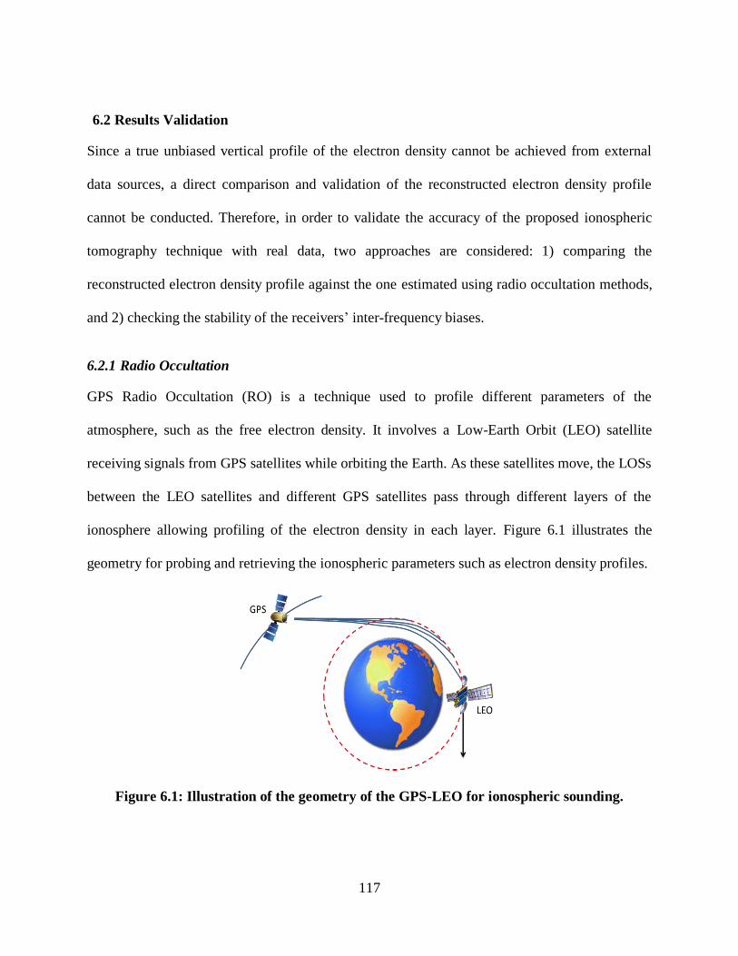
117
6.2 Results Validation
Since a true unbiased vertical profile of the electron density cannot be achieved from external
data sources, a direct comparison and validation of the reconstructed electron density profile
cannot be conducted. Therefore, in order to validate the accuracy of the proposed ionospheric
tomography technique with real data, two approaches are considered: 1) comparing the
reconstructed electron density profile against the one estimated using radio occultation methods,
and 2) checking the stability of the receivers’ inter-frequency biases.
6.2.1 Radio Occultation
GPS Radio Occultation (RO) is a technique used to profile different parameters of the
atmosphere, such as the free electron density. It involves a Low-Earth Orbit (LEO) satellite
receiving signals from GPS satellites while orbiting the Earth. As these satellites move, the LOSs
between the LEO satellites and different GPS satellites pass through different layers of the
ionosphere allowing profiling of the electron density in each layer. Figure 6.1 illustrates the
geometry for probing and retrieving the ionospheric parameters such as electron density profiles.
Figure 6.1: Illustration of the geometry of the GPS-LEO for ionospheric sounding.
118
The Constellation Observing System for the Meteorology, Ionosphere and Climate (COSMIC) is
one of several radio occultation missions where the data collected by GPS receivers onboard of
LEO satellites are post-processed and the electron density profiles are derived. The ionospheric
profiles of electron density (ionPrf) product can be downloaded at COSMIC website with a
reported accuracy of 0.1 – 1 1011
el/m3 (“COSMIC Program Office Website”, 2013). Many
authors have investigated the accuracy of electron density profile derived from radio occultation
measurements: Yue et al. (2013) reported an accuracy of 0.5 1011
el/m3
, Jakowski et al. (2005)
reported a systematic positive bias in the order of less than 0.8 1011
el/m3
and a standard
deviation of 1.3 1011
el/m3. In this research, the accuracy of 1 10
11 el/m
3 reported by COSMIC
Program Office Website is used as a reference of the accuracy measure of the radio occultation
retrieved electron density profiles. These profiles are used to validate the electron density
profiles reconstructed using the proposed ionospheric tomographic technique.
6.2.2 Stability of Receiver Inter-Frequency Biases (IFB)
STEC measurements are biased by the unknown satellite and receiver Inter-Frequency Biases
(IFB). The mean values of the biases are stable over a period of one day (Sardón and Zarraoa,
1997). This information can be useful to assess the solution of the proposed technique. Since the
main goal of the technique is to estimate the electron density using GPS data, it is possible to
reduce the number of unknowns and eliminate the IFB using a differencing technique explained
in Chapter 4. Once the electron density profiles are estimated, the residuals of Equation (4.22)
can be used to estimate the IFBs as follows:
(6.1)

119
(6.2)
where M, N, and P are the number of measurements, number of receivers, and number of
satellites used in the inversion, respectively. is a vector of the receiver and satellite inter-
frequency biases in units of TECU:
(6.3)
The design matrix is defined as:
(6.4)
where k = 1,2, … M, and q = 1,2,… (N+P), and i and j are the receiver and satellite indices used
to derive the kth
STEC measurement, respectively. For example, if N = 39 receivers and P = 10
satellites are used, then the kth
row of the design matrix F corresponding to measurement
derived using receiver i = 2 and satellite j = 2 is
1 N 1 P
(6.5)
120
In order to estimate the receiver and satellite inter-frequency biases, a reference (pseudo-
measurement) has to be introduced. This is due to the fact that the biases are relative values. One
approach, used by Jet Propulsion Laboratory (JPL), is to assume that the sum of all satellite inter-
frequency biases should be equal to zero. JPL estimates vertical TEC spatially and the inter-
frequency biases using stations over the globe, allowing them to observe all operational GPS
satellites. In this research, only the observations with LOS within the defined model space are
considered, where the LOS associated with each observation must enter the grid from the bottom
of the lowest layer and exit through the top of the highest layer as demonstrated in Chapter 4.
This results in a lower number of satellites available for analysis compared to JPL. Therefore,
another approach is adopted in this work where the summation of the satellites’ inter-frequency
biases is forced to be equal to the summation of the receiver inter-frequency biases. This will
yield a different solution than JPL’s (where the receiver inter-frequency biases absorb part of the
satellite inter-frequency biases). To eliminate this effect, the inter-frequency biases of two
receivers are differenced and the results are compared based on the relative inter-frequency
biases between different sites.
Applying the aforementioned approach results in a measurement vector with one more element
than the original observed :
(6.6)

121
and a design matrix F with one more row:
1 N 1 P
(6.7)
The inter-frequency biases are then estimated using the weighted least squares method described
in Chapter 4.
6.3 Data Description and Analysis Strategy
The GPS reference stations from CHAIN Network and the International GNSS Service (IGS) are
selected to assess the tomographic technique over Canadian polar region. The stations names and
geographic locations are listed in Table (5.1). Two types of STEC measurements are derived
from dual frequency GPS data: code-derived STEC and phase-derived STEC. The phase-derived
STEC is corrected for cycle slips, if possible, and then used to smooth the noisy code-derived
STEC, as described in Chapter 4. These measurements are used as input for the CIT model.
The developed CIT model estimates the electron density profiles and generates vertical TEC
maps using settings listed in Table 6.1, where one-hour data sets over a period of twenty four
hours of GPS data are processed. The results are then validated against the ionospheric profiles
of electron density generated by COSMIC Data Analysis and Archive Center (CDAAC) using
the radio occultation approach.

122
Table 6.1: Model settings
Nominal conditions
Region boundaries
= 45 N 80 N
= 240 E 304 E
height = 80 km 1180 km
Voxel spacing
( height) 1 4 25km
Duration 60 minutes
Data sampling rate Sample per 120 seconds
Cut-off angle 15
SCH pole 62.5 N and 272 E
SCH half-angle 27.5
Once the electron density distribution is estimated, the satellite and receiver inter-frequency
biases are estimated using the approach explained in the previous section. The stability of the
receiver inter-frequency biases, represented by the standard deviation, is analysed and a
comparison with a third party product, i.e. JPL, is conducted.
6.4 Constraining the Ionospheric Tomography Problem
The advantages of the proposed CIT technique have been discussed in Chapters 4 and 5. The low
number of required unknowns to represent the electron density profile and the low memory and
computation load using this technique make it a potential candidate as a tool for regional
ionospheric imaging. However, the ionospheric tomography technique is ill-conditioned and
singular. The design matrix is affected by small errors and the occurrence of outliers could affect
the solution significantly. An example of such an error is an undetected cycle slip. In addition to
the errors and outliers, the geometry plays an important role in achieving a reliable and realistic
solution. A realistic solution is an electron density profile that behaves as a Chapman-like profile
with all values being positive. Since ground-based GPS measurements are only used in this
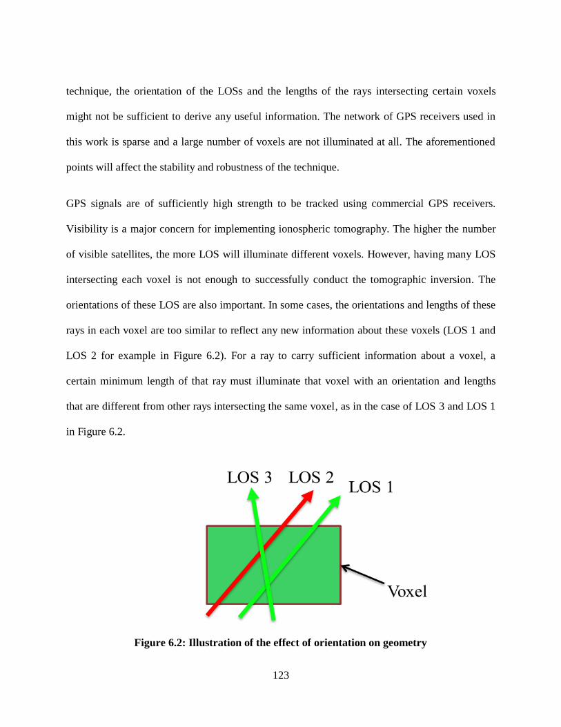
123
technique, the orientation of the LOSs and the lengths of the rays intersecting certain voxels
might not be sufficient to derive any useful information. The network of GPS receivers used in
this work is sparse and a large number of voxels are not illuminated at all. The aforementioned
points will affect the stability and robustness of the technique.
GPS signals are of sufficiently high strength to be tracked using commercial GPS receivers.
Visibility is a major concern for implementing ionospheric tomography. The higher the number
of visible satellites, the more LOS will illuminate different voxels. However, having many LOS
intersecting each voxel is not enough to successfully conduct the tomographic inversion. The
orientations of these LOS are also important. In some cases, the orientations and lengths of these
rays in each voxel are too similar to reflect any new information about these voxels (LOS 1 and
LOS 2 for example in Figure 6.2). For a ray to carry sufficient information about a voxel, a
certain minimum length of that ray must illuminate that voxel with an orientation and lengths
that are different from other rays intersecting the same voxel, as in the case of LOS 3 and LOS 1
in Figure 6.2.
Figure 6.2: Illustration of the effect of orientation on geometry
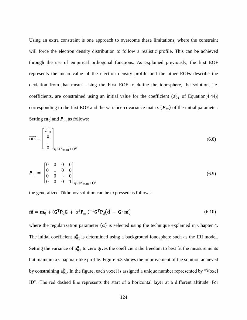
124
Using an extra constraint is one approach to overcome these limitations, where the constraint
will force the electron density distribution to follow a realistic profile. This can be achieved
through the use of empirical orthogonal functions. As explained previously, the first EOF
represents the mean value of the electron density profile and the other EOFs describe the
deviation from that mean. Using the First EOF to define the ionosphere, the solution, i.e.
coefficients, are constrained using an initial value for the coefficient ( of Equation(4.44))
corresponding to the first EOF and the variance-covariance matrix of the initial parameter.
Setting and as follows:
(6.8)
(6.9)
the generalized Tikhonov solution can be expressed as follows:
(6.10)
where the regularization parameter is selected using the technique explained in Chapter 4.
The initial coefficient is determined using a background ionosphere such as the IRI model.
Setting the variance of to zero gives the coefficient the freedom to best fit the measurements
but maintain a Chapman-like profile. Figure 6.3 shows the improvement of the solution achieved
by constraining . In the figure, each voxel is assigned a unique number represented by “Voxel
ID”. The red dashed line represents the start of a horizontal layer at a different altitude. For
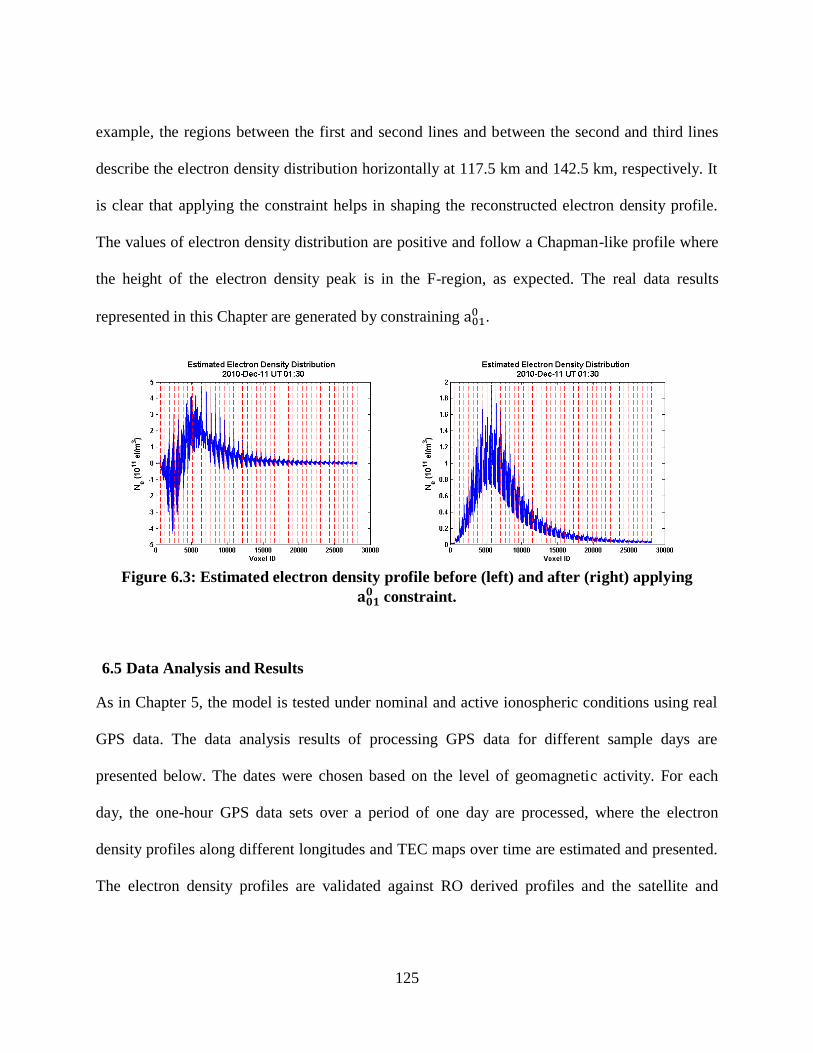
125
example, the regions between the first and second lines and between the second and third lines
describe the electron density distribution horizontally at 117.5 km and 142.5 km, respectively. It
is clear that applying the constraint helps in shaping the reconstructed electron density profile.
The values of electron density distribution are positive and follow a Chapman-like profile where
the height of the electron density peak is in the F-region, as expected. The real data results
represented in this Chapter are generated by constraining .
Figure 6.3: Estimated electron density profile before (left) and after (right) applying
constraint.
6.5 Data Analysis and Results
As in Chapter 5, the model is tested under nominal and active ionospheric conditions using real
GPS data. The data analysis results of processing GPS data for different sample days are
presented below. The dates were chosen based on the level of geomagnetic activity. For each
day, the one-hour GPS data sets over a period of one day are processed, where the electron
density profiles along different longitudes and TEC maps over time are estimated and presented.
The electron density profiles are validated against RO derived profiles and the satellite and

126
receiver inter-frequency biases are computed and their stability over the hours of the day is
checked.
6.5.1 Nominal Ionospheric Conditions
The geomagnetic activities on January 16, 2010, May 01, 2010 and December 11, 2010 are
shown in Figure 6.4. The activities are represented by a set of Kp indices. The Kp index is a
global indicator that reflects the geomagnetic activity level in a given three-hour time interval
(Gonzalez et al., 1994). It is derived using globally distributed (in longitude) sub-auroral ground-
based magnetometers. Kp indices range from 0 to 9. A Kp index can be interpreted as follows: a
value less than 4 indicates a low level of ionospheric activity, a value of 4 indicates a moderate
ionospheric level, and a value of 5 or greater indicates a storm level of geomagnetic activity;
however such values must be interpreted carefully since they reflect the global level of
geomagnetic activity but do not specify the region of high activity. As seen in the Figure, the Kp
index for the three selected dates ranges from 0 to 2 indicating a quiet nominal ionosphere.
The CIT-estimated vertical TEC maps for these dates are presented in Figure 6.5, Figure 6.6, and
Figure 6.7. The vertical TEC maps are obtained by integrating through the CIT-estimated
electron density profiles as described in Section 5.5. As expected, the results follow the expected
diurnal variation of TEC values with low values during nighttime and high values at the middle
of the day. The corresponding Root Mean Square (RMS) of the residuals is listed in Table 6.2.
The RMS increases for local times closer to the midday maximum peak ( ~20:30 UT). However,
the errors are no worse than ~2.5 TECU.

127
Figure 6.4: Planetary Kp indices for 16 January 2010 (top), 01 May 2010 (middle), and 11
December 2010 (bottom)
(http://www.swpc.noaa.gov/ftpmenu/warehouse/2011/2011_plots.html, April 2013)
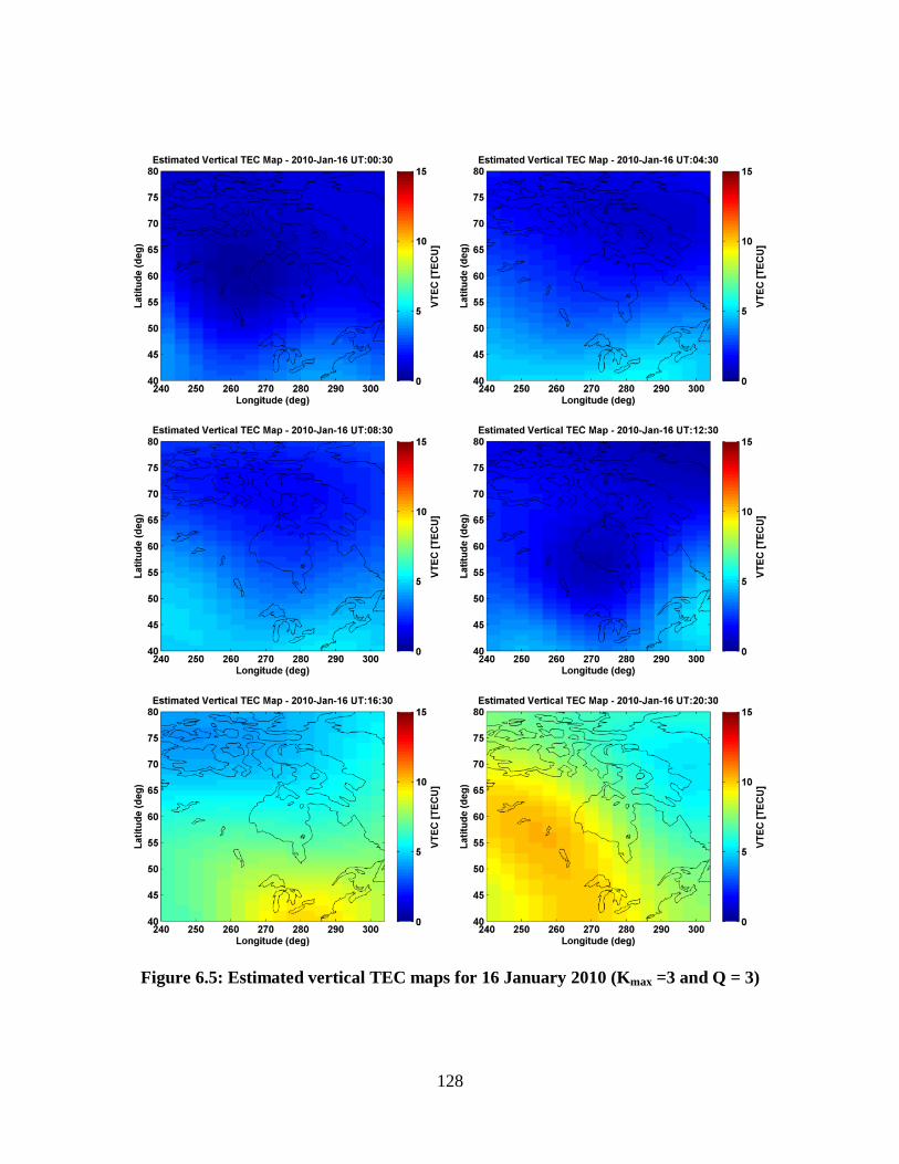
128
Figure 6.5: Estimated vertical TEC maps for 16 January 2010 (Kmax =3 and Q = 3)

129
Figure 6.6: Estimated vertical TEC maps for 01 May 2010 (Kmax =3 and Q = 3)

130
Figure 6.7: Estimated vertical TEC maps for 11 December 2010 (Kmax =3 and Q = 3)

131
Table 6.2: Root mean square of the residuals in TECU (Kmax =3 and Q = 3)
UTC 16 January
2010
01 May
2010
11 December
2010
00:30 1.19 2.00 1.70
04:30 1.87 1.86 1.85
08:30 1.89 1.37 1.70
12:30 1.67 1.89 1.91
16:30 1.75 1.47 1.68
20:30 2.07 2.39 1.93
6.5.1.1 Inter-Frequency Bias Stability
To conduct a quantitative assessment, the reconstruction result is first validated by examining the
relative inter-frequency receiver biases. Figure 6.8 shows a comparison of relative biases of JPL
versus the proposed technique for six IGS sites: ALGO, DRAO, CHUR, PRDS, HOLM and
YELL. The JPL relative inter-frequency receiver biases between DRAO and ALGO, CHUR and
ALGO, and CHUR and DRAO are –5.67 m, -3.54 m and -2.13 m, respectively. The JPL relative
inter-frequency receiver biases between YELL and HOLM, PRDS and HOLM, and PRDS and
YELL are –3.14 m, -1.14 m and -2.00 m, respectively. Comparing these values to the proposed
technique estimates, the receiver inter-frequency biases are consistent within 1.5 TECU (~24
cm).
The mean value of inter-frequency receiver biases is expected to be stable over the day on an
hour-to-hour basis. Therefore, this property can be used to determine accuracy of the ionosphere
reconstruction using the proposed technique. Processing one-hour data sets over a period of
twenty four hours, a measure of the stability can be computed by estimating the mean of the
inter-frequency receiver biases and their corresponding standard deviations. Table 6.3 shows the
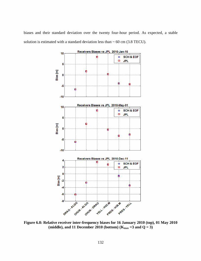
132
biases and their standard deviation over the twenty four-hour period. As expected, a stable
solution is estimated with a standard deviation less than ~ 60 cm (3.8 TECU).
Figure 6.8: Relative receiver inter-frequency biases for 16 January 2010 (top), 01 May 2010
(middle), and 11 December 2010 (bottom) (Kmax =3 and Q = 3)
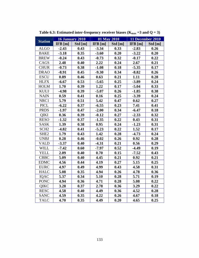
133
Table 6.3: Estimated inter-frequency receiver biases (Kmax =3 and Q = 3)
Station 16 January 2010 01 May 2010 11 December 2010
IFB [m] Std [m] IFB [m] Std [m] IFB [m] Std [m]
ALGO -2.43 0.43 -3.34 0.33 -2.83 0.26
BAKE -3.18 0.35 -3.60 0.20 -3.22 0.20
BREW -0.24 0.43 -0.73 0.32 -0.17 0.22
CAGS 2.48 0.40 2.22 0.24 2.67 0.21
CHUR -0.73 0.38 -1.08 0.18 -5.35 0.17
DRAO -8.91 0.45 -9.30 0.34 -8.82 0.26
ESCU 0.89 0.46 0.63 0.21 1.11 0.28
HLFX -6.67 0.53 -5.65 0.25 -3.89 0.24
HOLM 1.70 0.39 1.22 0.17 -5.04 0.33
KUUJ -4.98 0.39 -5.07 0.26 -1.85 0.38
NAIN 0.59 0.41 0.16 0.25 -3.39 0.24
NRC1 5.79 0.51 5.42 0.47 0.62 0.27
PICL -6.22 0.37 -6.55 0.23 7.41 0.41
PRDS -1.97 0.47 -2.00 0.34 -6.47 0.18
QIKI 0.36 0.39 -0.12 0.27 -2.33 0.32
RESO -1.32 0.37 -1.35 0.22 0.43 0.31
SASK 1.39 0.38 0.95 0.24 -1.23 0.31
SCH2 -4.82 0.41 -5.23 0.22 1.52 0.17
SHE2 1.79 0.43 1.42 0.28 -4.73 0.24
UNBJ 0.28 0.46 -0.02 0.26 0.92 0.28
VALD -3.37 0.40 -4.31 0.21 0.56 0.29
WILL -7.42 0.60 -7.97 0.52 -4.49 0.19
YELL 2.09 0.40 0.70 0.15 -7.52 0.43
CBBC 5.09 0.40 4.45 0.21 0.92 0.21
EDMC 4.56 0.44 4.19 0.27 5.15 0.25
EURC 4.97 0.49 4.99 0.43 4.58 0.31
HALC 5.08 0.35 4.94 0.26 4.78 0.36
IQAC 5.37 0.34 5.10 0.28 5.71 0.19
PONC 4.94 0.36 4.71 0.28 5.08 0.22
QIKC 3.28 0.37 2.78 0.36 3.29 0.22
RESC 4.58 0.40 4.49 0.36 4.52 0.28
SANC 4.59 0.35 4.22 0.26 4.67 0.18
TALC 4.70 0.35 4.49 0.20 4.65 0.25
134
6.5.1.2 Electron Density Profile Comparisons
The proposed CIT method estimates the electron density profile using GPS observations. To
further evaluate the performance of the method, radio occultation can be utilized and the CIT
derived electron density profile is compared to the one derived using radio occultation
measurements. Figure 6.9, Figure 6.10, and Figure 6.11 show four radio occultation events at
different hours of the day. Each plot consists of three subplots. The top left subplot shows the
geographical latitude and longitude of the perigee points. The green and red circles represent the
geographical horizontal coordinates of the first and last perigee points, respectively. The bottom
left subplot compares the electron density profiles derived using radio occultation (red) and
tomographic technique (blue). The subplot on the right shows the difference between the two
derived profiles. The red dotted line represent the accuracy range (± 1 1011
el/m3) of the radio
occultation derived electron density profile, as stated earlier in this Chapter.
The CIT derived electron density is defined at the centre of each voxel. To better compare and
validate the results, CIT derived profiles are interpolated and the electron density profiles are
computed at the geographical coordinates of the radio occultation perigee points. The error
statistics of a full day of radio occultation events are summarized in Table 6.4. It is found that the
CIT derived profile are biased by 0.3 1011
el/m3 with an overall RMS of ~0.5 10
11 el/m
3,
which is within the range of the radio occultation accuracy. For completeness, the mean and
RMS of the errors for all available occultation events for the selected dates are listed in Tables
6.5, 6.6, and 6.7.

135
Figure 6.9: Radio occultation (RO) vs. tomography (TOMO) electron density profiles for
16 January 2010
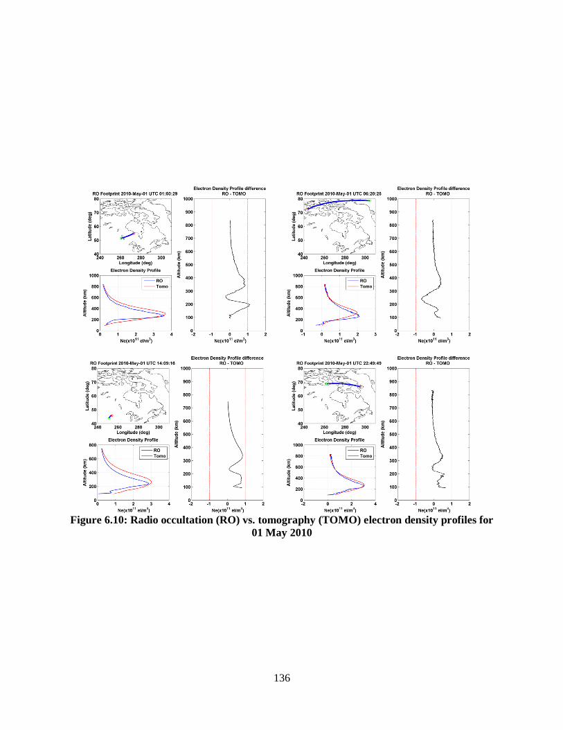
136
Figure 6.10: Radio occultation (RO) vs. tomography (TOMO) electron density profiles for
01 May 2010
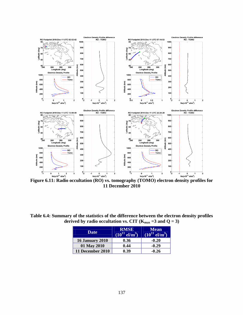
137
Figure 6.11: Radio occultation (RO) vs. tomography (TOMO) electron density profiles for
11 December 2010
Table 6.4: Summary of the statistics of the difference between the electron density profiles
derived by radio occultation vs. CIT (Kmax =3 and Q = 3)
Date RMSE
(1011
el/m3)
Mean
(1011
el/m3)
16 January 2010 0.36 -0.20
01 May 2010 0.44 -0.29
11 December 2010 0.39 -0.26

138
Table 6.5: Statistics of the difference between the electron density profiles derived by radio
occultation vs. CIT for 16 January 2010 (Kmax =3 and Q = 3)
UTC RMSE
(1011
el/m3)
Mean
(1011
el/m3)
UTC RMSE
(1011
el/m3)
Mean
(1011
el/m3)
00:06:48 0.33 -0.14 07:45:57 0.48 0.31
00:13:34 0.15 0.09 07:46:35 0.48 0.36
00:26:27 0.14 0.09 08:03:40 0.70 0.60
00:26:31 0.37 -0.21 08:07:29 0.68 0.55
00:27:13 0.37 -0.22 09:45:15 0.39 0.29
01:09:27 0.12 0.06 09:46:23 0.28 0.17
01:09:46 0.10 0.09 09:49:16 0.17 0.08
01:25:26 0.14 0.07 11:01:20 0.48 0.21
01:25:58 0.09 0.06 11:36:37 0.63 0.49
01:33:35 0.62 0.47 13:04:45 0.58 0.49
01:33:59 0.71 0.57 13:16:01 0.66 0.53
02:06:08 0.08 0.07 13:17:16 0.59 0.36
02:14:33 0.06 0.06 14:53:09 0.29 0.23
02:15:36 0.07 0.07 14:57:36 0.63 0.39
02:54:03 0.22 0.18 15:01:39 0.27 0.19
02:58:39 0.05 0.05 16:07:04 0.55 0.18
02:59:10 0.50 0.34 16:40:13 0.53 0.19
03:10:58 0.09 0.04 17:48:04 0.64 0.20
03:12:49 0.18 0.12 17:52:54 0.69 0.60
03:16:38 0.03 -0.02 18:02:32 0.50 0.18
03:54:01 0.09 0.06 18:06:07 0.66 0.48
03:56:41 0.10 0.09 18:11:46 0.15 0.15
04:15:57 0.11 0.06 18:33:30 0.70 0.52
04:42:26 0.45 0.30 19:29:12 0.58 0.35
04:42:46 0.46 0.35 19:30:19 0.56 0.37
04:42:46 0.40 0.31 19:33:43 0.49 0.35
04:48:26 0.19 0.15 19:40:41 0.09 0.08
04:54:46 0.36 0.26 19:42:55 0.45 0.14
04:55:20 0.46 0.33 19:44:01 0.44 0.23
05:44:40 0.21 0.09 19:50:41 0.49 0.37
05:59:29 0.32 -0.07 19:56:34 0.90 0.72
06:01:40 0.11 0.10 20:15:32 0.34 0.13
06:02:27 0.18 0.16 20:36:55 0.49 0.26
06:03:26 0.41 0.30 20:54:50 0.12 0.12
06:19:40 0.22 0.16 21:12:55 0.80 0.50
06:22:53 0.43 0.28 21:13:16 0.59 0.36
06:23:08 0.44 0.34 21:17:38 0.45 0.31
06:23:30 0.46 0.35 21:18:15 0.50 0.36
06:24:22 0.49 0.37 21:19:05 0.77 0.58
06:25:48 0.08 -0.08 21:22:11 0.20 0.20
07:21:42 0.16 0.10 21:31:17 0.96 0.71
07:28:13 0.51 0.40 21:31:17 0.63 0.50

139
Table 6.6: Statistics of the difference between the electron density profiles derived by radio
occultation vs. CIT for 01 May 2010 (Kmax =3 and Q = 3)
UTC
RMSE
(1011
el/m3)
Mean
(1011
el/m3)
UTC
RMSE
(1011
el/m3)
Mean
(1011
el/m3)
01:10:04 0.05 -0.05 08:07:16 0.24 0.17
01:11:13 0.38 0.23 09:44:33 0.27 0.22
01:50:29 0.39 0.26 09:54:16 0.13 0.11
02:06:17 0.41 0.04 10:47:49 0.25 0.01
02:40:16 0.07 -0.07 10:50:01 0.28 -0.18
02:51:24 0.81 0.66 12:47:55 0.16 0.09
02:54:28 0.28 0.09 14:09:16 0.44 0.35
04:25:11 0.14 0.13 14:12:58 0.20 0.12
04:28:02 0.46 0.33 14:14:57 0.32 0.24
04:36:11 0.50 0.37 14:16:14 0.25 -0.05
04:39:12 0.41 0.25 14:16:31 0.41 0.23
05:35:39 0.27 -0.03 16:39:38 0.46 0.21
05:40:24 0.38 0.29 17:35:41 0.33 0.05
05:50:34 0.33 0.22 17:47:04 0.81 0.10
05:53:40 0.08 0.07 18:19:07 0.04 0.03
06:20:00 0.62 0.56 19:28:34 0.55 -0.27
06:20:25 0.21 0.02 19:30:39 0.30 -0.05
06:23:01 0.52 0.42 21:02:08 0.04 0.00
06:24:49 0.40 0.25 21:02:44 0.34 0.04
06:27:27 0.38 0.22 21:04:28 0.02 0.01
06:31:33 0.07 0.07 22:33:20 0.57 0.52
07:16:25 0.05 -0.05 22:42:49 0.22 0.11
07:40:53 0.03 0.03 22:49:45 0.01 -0.01
07:43:24 0.22 0.17 22:49:49 0.21 0.08
07:43:44 0.42 0.42 22:57:33 0.53 0.19
07:54:20 0.33 0.15 23:00:35 0.56 0.37
08:02:05 1.01 0.93 23:03:02 0.60 0.41
08:07:13 0.74 0.70 23:09:27 0.11 0.09

140
Table 6.7: Statistics of the difference between the electron density profiles derived by radio
occultation vs. CIT for 11 December 2010 (Kmax =3 and Q = 3)
UTC RMSE
(1011
el/m3)
Mean
(1011
el/m3)
UTC RMSE
(1011
el/m3)
Mean
(1011
el/m3)
01:17:05 0.07 0.06 07:48:50 0.35 0.26
02:02:42 0.30 0.19 07:49:50 0.04 0.04
02:13:26 0.96 0.80 07:50:39 0.11 0.11
02:14:14 0.86 0.73 09:15:05 0.20 0.19
02:20:38 0.27 0.18 09:22:09 0.47 -0.47
02:21:47 0.25 0.17 09:27:06 0.64 0.47
03:49:12 0.58 0.40 12:50:09 0.77 0.45
03:56:21 0.21 0.20 12:59:51 0.39 0.18
04:00:40 0.54 0.45 13:00:49 0.63 0.40
04:06:32 0.42 0.24 13:05:08 0.79 0.58
04:10:24 0.02 -0.02 13:06:02 0.16 0.16
05:47:48 0.42 0.29 16:24:48 0.82 0.35
05:46:03 0.52 0.37 17:12:17 1.38 0.95
05:51:09 0.03 0.01 20:22:21 0.71 0.37
05:46:28 0.17 0.15 20:35:27 0.74 0.42
05:48:47 0.36 0.27 20:37:28 0.82 0.44
05:58:05 0.64 0.49 20:40:25 0.29 0.09
05:59:23 0.48 0.35 20:43:18 0.05 0.04
07:14:53 0.10 0.03 22:03:24 1.15 0.25
07:16:24 0.16 0.09 22:12:20 0.39 0.22
07:32:01 0.17 0.12 22:20:54 0.52 0.27
07:33:16 0.22 0.19

141
6.5.2 Disturbed Ionospheric Conditions
To assess the performance of the proposed CIT technique under more challenging conditions,
GPS data during a period of enhanced ionospheric activity are processed and the CIT estimated
profiles are validated. Initially, the disturbed day was chosen based on the Kp index. A Kp index
higher than 4 indicates potentially disturbed local ionospheric conditions. After a thorough
search in the Kp index of the years 2010 and 2011, it was found that 9 and 10 September, 2011
had a period with a Kp index that meets this criteria. Figure 6.12 shows the Kp index from 8 to
10 September, 2011. A Kp index of 7 was recorded after extremely quiet conditions. This is a
strong indication that a geomagnetic storm was in progress. However, the Kp index is derived
from globally distributed ground-based magnetometers. It reflects the conditions in a global
sense and does not indicate where the activity is taking place. Therefore, another indicator (K-
index) is required to confirm the disturbed conditions over a local region such as the Canadian
polar region. The Canadian Geomagnetism Program computes the K-indices for three Canadian
observatories: Ottawa (OTT), Meanook (MEA), and Victoria (VIC). Figure 6.13 shows the K-
indices at these observatories for 09 and 10 September, 2011. It can be seen that K-indices of 4
or greater were recorded on 09 and 10 September, 2011. Specifically, the K-index at MEA
ranges between 5 and 7 during the period of interest confirming that the ionosphere was
disturbed during these days. As a result, the GPS data of 10 September are processed for the 24
hours of day as in the case of quiet days and the results are presented below.

142
Figure 6.12: Planetary Kp indices for 10 September 2011
(http://www.swpc.noaa.gov/ftpmenu/warehouse/2011/2011_plots.html, April 2013)
Figure 6.13: Local K-index for 9-10 September, 2011 (data courtesy of NRCAN)

143
Figure 6.15 shows the vertical TEC maps at selected hours of the day. The maps show the
expected diurnal variation with no negative TEC values. The RMS of the residuals (Table 6.8)
are noticeably high (~4 TECU) for UTC 00:30 and are generally higher than those computed for
quiet days (Table 6.2). This can be explained by considering Figure 6.14 which shows the
geomagnetic field observations at several Magnetic Observatories across Canada. The
observations agree with the local K-index , where a variation along the North-South magnetic
field component was persistent and lasted for the first ~10 hours for most of the stations
especially those located between 49.5 N and 62.5 N and 246 E and 291.5 E. High
fluctuations and sharp spikes in the geomagnetic field were detected especially in the first two
hours of the day. During the same period, a local K-index value of 7 was recorded at MEA. This
indicates a higher local level of geomagnetic activity occurred during these hours, which resulted
in higher TEC residuals.
Figure 6.14: Geomagnetic field observations for Canadian magnetic observatories for 10
September, 2011 (http://www.geomag.nrcan.gc.ca; April 2013)

144
Figure 6.15: Estimated vertical TEC maps for 10 September 2011 (Kmax =3 and Q = 3)

145
Table 6.8: Root mean square of the residuals in TECU (Kmax =3 and Q = 3)
UTC 10 September
2010
00:30 4.03
04:30 2.31
08:30 2.19
12:30 1.94
16:30 2.02
20:30 2.76
Comparing the CIT electron density profiles to the RO-derived electron density profiles, the
errors statistics of the full day of radio occultation events are found to be biased by 0.1 1011
el/m3 with an overall root mean square of the errors of ~0.6 10
11 el/m
3, which is slightly higher
than that computed for the quiet days but within the range of the radio occultation accuracy. The
estimated receiver IFB are listed in Table 6.9 and found to be stable with a standard deviation
less than ~60 cm (3.8TECU). Comparison of the relative biases for JPL versus the proposed CIT
technique (for the same sites analysed in Section 6.5) is presented in Figure 6.16 and results are
consistent within 1.44 TECU (~23 cm). For completeness, the statistics of the difference between
the electron density profiles derived by radio occultation versus CIT for all available occultation
events are listed in Table 6.10.

146
Figure 6.16: Comparison of JPL relative receiver inter-frequency biases for 10 September
2011 (Kmax =3 and Q = 3)
Table 6.9: Estimated inter-frequency receiver biases for 10 September 2011 (Kmax =3 and Q
= 3)
Station IFB [m] Std [m] Station IFB [m] Std [m]
ALGO -2.55 0.57 SASK 2.36 0.38
BAKE -3.05 0.24 SCH2 -5.50 0.27
BREW 0.07 0.56 SHE2 1.09 0.44
CHUR -5.84 0.31 UNBJ 0.68 0.39
DRAO -8.05 0.55 VALD -4.15 0.37
ESCU 1.61 0.39 WILL -6.92 0.58
FLIN -7.83 0.38 YELL 1.34 0.26
HLFX -4.73 0.43 CBBC 4.89 0.33
HOLM -1.85 0.30 EDMC 5.07 0.45
KUUJ -3.03 0.31 EURC 5.34 0.51
NAIN 1.12 0.30 HALC 5.52 0.34
NRC1 6.53 0.48 IQAC 5.58 0.31
PICL -5.59 0.34 PONC 5.20 0.38
PRDS -0.63 0.46 RESC 4.84 0.44
QIKI 1.45 0.36 SANC 5.08 0.26
RESO -0.84 0.36 TALC 4.89 0.31
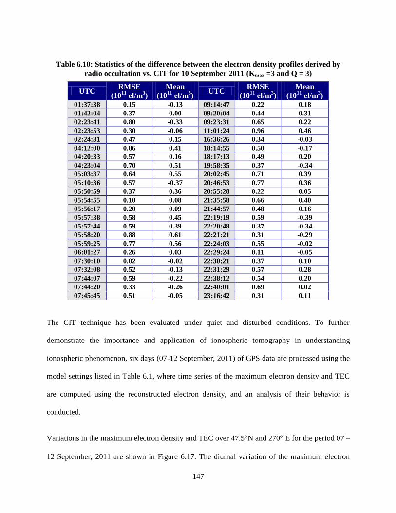
147
Table 6.10: Statistics of the difference between the electron density profiles derived by
radio occultation vs. CIT for 10 September 2011 (Kmax =3 and Q = 3)
UTC RMSE
(1011
el/m3)
Mean
(1011
el/m3)
UTC RMSE
(1011
el/m3)
Mean
(1011
el/m3)
01:37:38 0.15 -0.13 09:14:47 0.22 0.18
01:42:04 0.37 0.00 09:20:04 0.44 0.31
02:23:41 0.80 -0.33 09:23:31 0.65 0.22
02:23:53 0.30 -0.06 11:01:24 0.96 0.46
02:24:31 0.47 0.15 16:36:26 0.34 -0.03
04:12:00 0.86 0.41 18:14:55 0.50 -0.17
04:20:33 0.57 0.16 18:17:13 0.49 0.20
04:23:04 0.70 0.51 19:58:35 0.37 -0.34
05:03:37 0.64 0.55 20:02:45 0.71 0.39
05:10:36 0.57 -0.37 20:46:53 0.77 0.36
05:50:59 0.37 0.36 20:55:28 0.22 0.05
05:54:55 0.10 0.08 21:35:58 0.66 0.40
05:56:17 0.20 0.09 21:44:57 0.48 0.16
05:57:38 0.58 0.45 22:19:19 0.59 -0.39
05:57:44 0.59 0.39 22:20:48 0.37 -0.34
05:58:20 0.88 0.61 22:21:21 0.31 -0.29
05:59:25 0.77 0.56 22:24:03 0.55 -0.02
06:01:27 0.26 0.03 22:29:24 0.11 -0.05
07:30:10 0.02 -0.02 22:30:21 0.37 0.10
07:32:08 0.52 -0.13 22:31:29 0.57 0.28
07:44:07 0.59 -0.22 22:38:12 0.54 0.20
07:44:20 0.33 -0.26 22:40:01 0.69 0.02
07:45:45 0.51 -0.05 23:16:42 0.31 0.11
The CIT technique has been evaluated under quiet and disturbed conditions. To further
demonstrate the importance and application of ionospheric tomography in understanding
ionospheric phenomenon, six days (07-12 September, 2011) of GPS data are processed using the
model settings listed in Table 6.1, where time series of the maximum electron density and TEC
are computed using the reconstructed electron density, and an analysis of their behavior is
conducted.
Variations in the maximum electron density and TEC over 47.5N and 270 E for the period 07 –
12 September, 2011 are shown in Figure 6.17. The diurnal variation of the maximum electron

148
density and TEC is evident in the figure, where the lowest and highest values are expected
during nighttime and 14:00 LT (20:00 UT along meridian 270 E), respectively. However, an
unexpected sudden increase and gradual decrease in these values can be clearly seen on 9
September. Such behavior may indicate that ionospheric activity, such as ionospheric storm, is in
progress.
Ionospheric storm resembles the magnetic storm. The storm effects are observed at high and
middle latitude (Hargreaves, 1995). It is characterized by variations in and TEC. There
are three phases in the ionospheric storm: positive phase, main phase, and recovery phase. The
positive phase, lasting a few hours, is characterized by an initial growth in the electron density
and the total electron content. As the electron density distribution reaches values greater than
normal, the main (negative) phase starts where a decrease in the electron density below normal
values is evident. The electron density gradually returns to normal levels in the recovery phase,
which might last for a period of one or more days.
Ionospheric storms occur in conjunction with geomagnetic storms. Therefore, a confirmation of
the occurrence of a geomagnetic storm is necessary and the behavior of the maximum electron
density is studied according to the definition of ionospheric storm where the positive and
negative phases are identified. Different observations and indicators are used to confirm the
signature associated with the geomagnetic storm. These include geomagnetic field observations,
Disturbed Storm Time (Dst) index, Interplanetary Magnetic Field (IMF), and solar wind
velocity.

149
Figure 6.17: Vertical TEC (top) and Nemax (bottom) over 47.5N and 270 E for September
2011
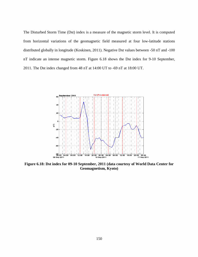
150
The Disturbed Storm Time (Dst) index is a measure of the magnetic storm level. It is computed
from horizontal variations of the geomagnetic field measured at four low-latitude stations
distributed globally in longitude (Koskinen, 2011). Negative Dst values between -50 nT and -100
nT indicate an intense magnetic storm. Figure 6.18 shows the Dst index for 9-10 September,
2011. The Dst index changed from 48 nT at 14:00 UT to -69 nT at 18:00 UT.
Figure 6.18: Dst index for 09-10 September, 2011 (data courtesy of World Data Center for
Geomagnetism, Kyoto)
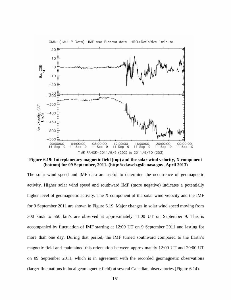
151
Figure 6.19: Interplanetary magnetic field (top) and the solar wind velocity, X component
(bottom) for 09 September, 2011. (http://cdaweb.gsfc.nasa.gov; April 2013)
The solar wind speed and IMF data are useful to determine the occurrence of geomagnetic
activity. Higher solar wind speed and southward IMF (more negative) indicates a potentially
higher level of geomagnetic activity. The X component of the solar wind velocity and the IMF
for 9 September 2011 are shown in Figure 6.19. Major changes in solar wind speed moving from
300 km/s to 550 km/s are observed at approximately 11:00 UT on September 9. This is
accompanied by fluctuation of IMF starting at 12:00 UT on 9 September 2011 and lasting for
more than one day. During that period, the IMF turned southward compared to the Earth’s
magnetic field and maintained this orientation between approximately 12:00 UT and 20:00 UT
on 09 September 2011, which is in agreement with the recorded geomagnetic observations
(larger fluctuations in local geomagnetic field) at several Canadian observatories (Figure 6.14).

152
All the above space weather parameters clearly confirm signatures of a geomagnetic storm on 9-
10 September, 2011. Referring to Figure 6.17, the sudden increase of TEC and values are
consistent with the geomagnetic storm signatures. The positive and main storm phases can be
identified in the figure. During the positive phase, the maximum electron density reached a value
of ~ 10 1011
el/m3
on 09 September at 18:30 UT, which is twice the value of the previous days
(~5. 1011
el/m3). The main phase followed the positive values, where the maximum electron
density values decrease gradually and return to normal levels after one day. The values of TEC
behave similarly.
6.6 Chapter Summary
The CIT technique has been tested and validated under quiet and disturbed ionospheric
conditions using GPS real data. An additional constraint is introduced as a suggested approach to
overcome the effect of bad data geometry and undetected errors on the inversion problem.
Results based on this method are presented. The estimated vertical TEC maps show the expected
diurnal variation with realistic (no negative) TEC values. The relatively good comparison
between the CIT-estimated electron density profiles and the RO derived profiles, combined with
the relatively stable IFB and small differences between JPL and CIT-estimated relative IFB
proves the validity of the technique and the correct implementation of the algorithm. A study of
an ionospheric storm using CIT has been conducted. The phases of the ionospheric storm were
identified based on the TEC and maximum electron density estimated using CIT. The study
demonstrates that GPS tomography has become regarded as a useful tool in monitoring the
ionosphere and providing a better understanding of the physical processes occurring in the
Canadian polar region.
153
Chapter Seven: Conclusions and Recommendations
Ionospheric imaging over the Canadian polar region using GPS observations has been
investigated in this thesis. The following sections summarize the conclusions and
recommendations for future work.
7.1 Conclusions
A new three-dimensional Computerized Ionospheric Tomographic (CIT) technique using GPS
measurements has been developed. The technique uses a combination of Spherical Cap
Harmonics (SCH) and Empirical Orthogonal Functions (EOF) to describe the electron density
distribution. The spherical cap harmonics describe the electron distribution horizontally and the
empirical orthogonal functions describe and constrain the electron density distribution vertically.
The vertical constraint is necessary in the case of using only ground-based GPS measurements so
that a certain range of possible realistic solutions is allowed.
The algorithm has been implemented in a MATLAB software package. The software package
takes in GPS data and applies the technique over a region bounded by latitude, longitude and
altitude. Different settings can be set in the program. Some of these parameters are the cutoff
angle, GPS data sampling interval, number of EOF (Q) and order of spherical cap harmonics
( , spherical cap half-angle (o), and many others.
The feasibility of the new technique has been demonstrated using simulated data. The
International Reference Ionosphere (IRI) model is used to simulate the electron density
distribution in the ionosphere. Different ionospheric conditions have been simulated to assess the
performance of the model in recovering different ionospheric parameters such as the electron
density and Total Electron Content (TEC). These conditions are chosen so that the technique can
154
represent nominal and storm conditions. The purpose of these simulation are: 1) determine the
most appropriate combination of and Q for the Canadian polar region to be adopted for
processing GPS real data, and 2) demonstrate and assess the performance of the new technique.
A network of existing GPS stations and simulated ionospheric conditions using IRI-2007 are
used to determine the most appropriate combination of and Q for the Canadian polar region
which is found to be 3 and 3, respectively. The model is successful in retrieving the electron
density profiles under nominal conditions. However, the technique cannot replicate and
reconstruct electron density profiles that meet the targeted performance metrics under
challenging conditions, such as the Storm Enhanced Density (SED). To overcome this limitation,
a new approach has been proposed where the solution of the CIT technique is used to constrain
the ionospheric tomography in its original form (voxel-based model). The high computational
load and memory requirement associated with this approach is still a major concern and imposes
a limitation in applying the method especially if a higher resolution, i.e. higher number of voxels,
is required.
GPS real data has been used to further validate the CIT technique under quiet and disturbed
conditions. However, in addition to the bad geometry associated with sparse GPS network
stations, GPS-derived STEC measurements are susceptible to cycle slips and highly affected by
noise. Since the design matrix associated with tomographic inversion is singular and severely ill-
conditioned, the solutions estimated in such cases are not accurate and might be physically
unrealistic. Therefore, an additional constraint has been proposed and introduced to enforce the
technique to produce physically realistic solutions. In addition to this constraint, a reference
(pseudo TEC measurement) has been introduced to estimate the receiver and satellite Inter-

155
Frequency Biases (IFB). The results are validated using: 1) Radio Occultation (RO) products;
and 2) testing the stability of the IFB. Results shows expected diurnal variation of TEC values.
The electron density profiles are relatively comparable to the RO derived profiles product within
the reported accuracy of the product. The CIT-estimated IFB are found to be stable over the day
and close to the values reported by Jet Propulsion Laboratory (JPL), indicating the validity and
correct implementation of the technique. A study of an ionospheric storm has been conducted to
demonstrate the importance of GPS tomography in identifying such events and providing a cost
effective tool to remotely sense the Earth’s ionosphere - which helps to better understand the
physical processes in the ionosphere.
7.2 Recommendations
Ionospheric imaging using tomography is an ill-posed ill-conditioned inverse problem. This
problem is mixed-determined: that is there are regions where the measurements over-determine
some of the components in the solution, but under-determine other components. This is due to
the sparsity and lack of data in certain regions. For example, there are no receivers in oceans and
seas. This makes the ionosphere difficult to monitor by the data alone. Also, as explained in
Chapter 4, the data geometry involved in ionospheric tomography using only ground-based GPS
measurements is not ideal. Observations over all possible angles are not possible. There are
insufficient measurements (line of sights) perpendicular to altitude; therefore the vertical
resolution is not as good as the horizontal resolution. These issues impose certain limitations in
the resolution and accuracy of the ionospheric tomography solution. A possible solution to these
limitations is the use of some a priori information. The approach adopted in the thesis work
utilizes empirical orthogonal functions to incorporate some a priori information on the vertical
156
distribution of the electron density. However, combining different data sources that provide
horizontal information can improve the vertical resolution. Satellite-based observations such as
those from COSMIC provide additional observations which have good altitude information that
help increase the coverage of the topside ionosphere data (that is so important for vertical
resolution in the images). Thus, the limitations of sparsity of data and lack of vertical resolution
in 3-D ionospheric tomographic imaging can be addressed through the ongoing development and
availability of new and additional data sources. The new European satellite navigation system,
Galileo, and the restored Russian system, GLONASS, are examples of other constellations that
can double the quantity of TEC data, increasing the data coverage for such imaging.
The focus of the thesis is to develop an optimal tomographic model for the Canadian polar
region to estimate ionospheric parameters that help in understanding the ionosphere better at
such high latitudes. The technique shows promising results. Further investigations should be
conducted for different wide area GPS networks at different latitudes with higher reference
station density; investigations should include feasibility of the technique and the effect of
different parameters on the model accuracy (such as cuttoff angle and site spacing). Studies
should include Kmax and Q as a function of network size, density of receivers, voxel size, polar
cap parameters, and latitude and ionospheric activity.
Although the main product of the model is electron density, TEC maps can be computed and
ionospheric corrections for navigation applications can be generated. The quality of the maps,
hence the ionospheric corrections, are expected to be better than the conventional TEC maps
generated from two-dimensional modelling. Further investigation of the quality of CIT derived
ionospheric corrections for wide area GPS networks is recommended.
157
References
Afraimovich, E.L., Pirog, O.M. and Terekhov, A.I. (1992), “Diagnostics of large-scale structures
of the high-latitude ionosphere based on tomographic treatment of navigation-satellite
signals and of data from ionospheric stations”, Journal of Atmospheric and Terrestrial
Physics, Vol. 54 No. 10, pp. 1265–1273.
AIAA. (1999), AIAA Guide to Reference and Standard Ionosphere Models, AIAA (American
Institute of Aeronautics and Astronautics).
Araujo-Pradere, E.A., Fuller-Rowell, T.J., Codrescu, M.V. and Bilitza, D. (2005),
“Characteristics of the ionospheric variability as a function of season, latitude, local time,
and geomagnetic activity”, Radio Science, Vol. 40 No. 5, p. RS5009.
Arikan, O., Arikan, F. and Erol, C.B. (2007), “Computerized ionospheric tomography with the
IRI model”, Advances in Space Research, Vol. 39 No. 5, pp. 859–866.
Aster, R.C., Borchers, B. and Thurber, C.H. (2012), Parameter Estimation and Inverse
Problems, Academic Press.
Austen, J.R., Franke, S.J. and Liu, C.H. (1988), “Ionospheric imaging using computerized
tomography”, Radio Science, Vol. 23 No. 3, pp. 299–307.
Austen, J.R., Franke, S.J., Liu, C.H. and Yeh, K.C. (1986), “Application of computerized
tomography techniques to ionospheric research”, Presented at the International Beacon
Satellite Symposium on Radio Beacon Contribution to the Study of Ionization and
Dynamics of the Ionosphere and to Corrections to Geodesy and Technical Workshop, pp.
25–35.

158
Bhuyan, K., Singh, S.B. and Bhuyan, P.K. (2002), “Tomographic reconstruction of the
ionosphere using generalized singular value decomposition”, Current Science, Vol. 83
No. 9, pp. 1117–1120.
Bhuyan, K., Singh, S.B. and Bhuyan, P.K. (2004), “Application of generalized singular value
decomposition to ionospheric tomography”, Ann. Geophys., Vol. 22 No. 10, pp. 3437–
3444.
Bilitza, D. and Reinisch, B.W. (2008), “International Reference Ionosphere 2007: Improvements
and new parameters”, Advances in Space Research, Vol. 42, pp. 599–609.
Bjõrck, A. (1996), Numerical Methods for Least Squares Problems, SIAM.
Brunini, C.A. (1998), Global ionospheric model from GPS measurements (Ph.D. thesis, Facultad
de Ciencias Astronomicas y Geofisicas, La Plata, Argentina), Facultad de Ciencias
Astronomicas y Geofisicas, La Plata, Argentina.
Bust, G.S., Garner, T.W. and Gaussiran II, T.L. (2004), “Ionospheric Data Assimilation Three-
Dimensional (IDA3D): A global, multisensor, electron density specification algorithm”,
Journal of Geophysical Research, Vol. 109 No. A11, p. A11312.
Bust, G.S. and Mitchell, C.N. (2008), “History, current state, and future directions of ionospheric
imaging”, Reviews of Geophysics, Vol. 46 No. 1, p. RG1003.
Ciraolo, L., Azpilicueta, F., Brunini, C., Meza, A. and Radicella, S.M. (2007), “Calibration
errors on experimental slant total electron content (TEC) determined with GPS”, Journal
of Geodesy, Vol. 81, pp. 111–120.
Colombo, O.L., Hernandez-Pajares, M., Juan, J.M. and Sanz, J. (2000), “Ionospheric
tomography helps resolve GPS ambiguities on the fly at distances of hundreds of
kilometers during increased geomagnetic activity”, Position Location and Navigation

159
Symposium, IEEE 2000, Presented at the Position Location and Navigation Symposium,
IEEE 2000, pp. 15–21.
“COSMIC Program Office Website”. (2013), . Retrieved from http://cdaac-
www.cosmic.ucar.edu/cdaac/products.html
Coster, A. and Skone, S. (2009), “Monitoring storm-enhanced density using IGS reference
station data”, Journal of Geodesy, Vol. 83 No. 3-4, pp. 345 – 351.
Coster, A.J., Colerico, M.J., Foster, J.C., Rideout, W. and Rich, F. (2007), “Longitude sector
comparisons of storm enhanced density”, Geophysical Research Letters, Vol. 34 No. 18,
p. L18105.
Daniell, R.E., Brown, L.D., Anderson, D.N., Fox, M.W., Doherty, P.H., Decker, D.T., Sojka,
J.J., et al. (1995), “Parameterized ionospheric model: A global ionospheric
parameterization based on first principles models”, Radio Science, Vol. 30 No. 5, pp.
1499–1510.
Erturk, O., Arikan, O. and Arikan, F. (2009), “Tomographic reconstruction of the ionospheric
electron density as a function of space and time”, Advances in Space Research, Vol. 43
No. 11, pp. 1702–1710.
ESA. (2013,April), “European Space Agency”, http://www.egnos-pro.esa.int/index.html.
FAA. (2013,April), “Federal Aviation Administration (FAA)”, http://www.faa.gov.
Foster, J.C. (1993), “Storm time plasma transport at middle and high latitudes”, Journal of
Geophysical Research, Vol. 98 No. A2, pp. 1675–1689.
Foster, J.C. (2000), “Quantitative Investigation of Ionospheric Density Gradients at Mid
Latitudes”, Presented at the Proceedings of the 2000 National Technical Meeting of The
Institute of Navigation, Anaheim, CA, pp. 447–453.
160
Fremouw, E.J., Secan, J.A. and Howe, B.M. (1992), “Application of stochastic inverse theory to
ionospheric tomography”, Radio Science, Vol. 27 No. 5, pp. 721–732.
Gonzalez, W.D., Joselyn, J.A., Kamide, Y., Kroehl, H.W., Rostoker, G., Tsurutani, B.T. and
Vasyliunas, V.M. (1994), “What is a geomagnetic storm?”, Journal of Geophysical
Research: Space Physics, Vol. 99 No. A4, pp. 5771–5792.
“GPS Official Website”. (2013), . Retrieved from http://www.gps.gov/
Haines, G.V. (1985), “Spherical cap harmonic analysis of geomagnetic secular variation over
Canada 1960–1983”, Journal of Geophysical Research: Solid Earth, Vol. 90 No. B14,
pp. 12563–12574.
Hargreaves, J.K. (1995), The Solar-Terrestrial Environment: An Introduction to Geospace - the
Science of the Terrestrial Upper Atmosphere, Ionosphere, and Magnetosphere,
Cambridge University Press.
Hernández-Pajares, M., Juan, J.M., Sanz, J. and Colombo, O.L. (2000), “Application of
ionospheric tomography to real-time GPS carrier-phase ambiguities Resolution, at scales
of 400-1000 km and with high geomagnetic activity”, Geophysical Research Letters, Vol.
27, pp. 2009–2012.
Hofmann-Wellenhof, B., Lichtenegger, H. and Wasle, E. (2007), GNSS - Global Navigation
Satellite Systems: GPS, GLONASS, Galileo, and more, Springer, 8thed.
Hofman-Wellenhof, B., Lichtenegger, H. and Collins, J. (2001), Global Positioning System:
Theory and Practice, Springer Wien, 5thed.
“Interface Specification, IS-GPS-200F”. (2011), . Retrieved from
http://www.gps.gov/technical/icwg/ISGPS-200F.pdf

161
Jakowski, N., Tsybulyal, K., Radicella, S.M., Cueto, M. and Herraiz, M. (2005), “Comparison of
Electron Density Profiles from CHAMP Data with NeQuick Model”, in Reigber,
P.D.D.C., Lühr, P.D.H., Schwintzer, D.P. and Wickert, D.J. (Eds.),Earth Observation
with CHAMP, Springer Berlin Heidelberg, pp. 483–488.
Jayachandran, P.T., Langley, R.B., MacDougall, J.W., Mushini, S.C., Pokhotelov, D., Hamza,
A.M., Mann, I.R., et al. (2009), “Canadian High Arctic Ionospheric Network (CHAIN)”,
Radio Science, Vol. 44 No. 1, p. RS0A03.
Kaplan, E.D. (2005), Understanding GPS: Principles and Applications, (Kaplan, E.D. and
Hegarty, C.,Eds.), Artech House, 2nded.
Kelley, M.C. (2009), The Earth’s Ionosphere: Plasma Physics & Electrodynamics, Academic
Press.
Kleusberg, A. and Teunissen, P.J.G. (1998), GPS for geodesy, Springer.
Komjathy, A. (1997,September), Global ionospheric total electron content mapping using the
global positioning system, Department of Geodesy and Geomatics Engineering,
University of New Brunswick.
Koskinen, H. (2011), Physics of Space Storms: From the Surface of the Sun to the Earth,
Springer.
Liu, J., Chen, R., Kuusniemi, H., Wang, Z., Zhang, H. and Yang, J. (2009), “Mapping the
regional ionospheric TEC using a spherical cap harmonic model and IGS products in
high latitudes and the arctic region”, Proceedings of IAIN 2009 World Congress,
Stockholm, Sweden.
Liu, Z. and Gao, Y. (2004), “Development and Evaluation of a New 3-D Ionospheric Modeling
Method”, Navigation, Vol. 51 No. 4, pp. 311–329.

162
Materassi, M. and Mitchell, C.N. (2005), “A simulation study into constructing of the sample
space for ionospheric imaging”, Journal of atmospheric and solar-terrestrial physics,
Vol. 67 No. 12, pp. 1085–1091.
Mead, J.L. (2007), “Parameter estimation: A new approach to weighting a priori information”, J.
Inv. Ill-Posed Problems, Vol. 15, pp. 1–21.
Meggs, R.W. and Mitchell, C.N. (2006), “A study into the errors in vertical total electron content
mapping using GPS data”, Radio Science, Vol. 41 No. 1, p. RS1008.
Meggs, R.W., Mitchell, C.N. and Spencer, P.S.J. (2004), “A comparison of techniques for
mapping total electron content over Europe using GPS signals”, Radio Science, Vol. 39
No. 1, p. RS1S10.
Misra, P. and Enge, P. (2006), Global positioning system: signals, measurements, and
performance, Ganga-Jamuna Press.
Mitchell, C.N. and Spencer, P.S.J. (2003), “A three-dimensional time-dependent algorithm for
ionospheric imaging using GPS”, Annals of Geophysics. Retrieved from
http://www.earth-prints.org/handle/2122/977
Parkinson, B.W. and Spilker, J.J. (Eds.). (1996), Global Positioning System: Theory &
Applications (Volume One), American Institute of Aeronautics and Astronautics, 1sted.
Pryse, S.E. and Kersley, L. (1992), “A preliminary experimental test of ionospheric
tomography”, Journal of Atmospheric and Terrestrial Physics, Vol. 54 No. 7–8, pp.
1007–1012.
Rao, G.S. (2010), Global Navigation Satellite Systems, Tata McGraw-Hill Education.

163
Raymund, T.D., Pryse, S.E., Kersley, L. and Heaton, J. a. T. (1993), “Tomographic
reconstruction of ionospheric electron density with European incoherent scatter radar
verification”, Radio Science, Vol. 28 No. 5, pp. 811–817.
Rius, A., Ruffini, G. and Cucurull, L. (1997), “Improving the vertical resolution of ionospheric
tomography with GPS Occultations”, Geophysical Research Letters, Vol. 24 No. 18, pp.
2291–2294.
Rogers, N.C., Mitchell, C.N., Heaton, J. a. T., Cannon, P.S. and Kersley, L. (2001), “Application
of radio tomographic imaging to HF oblique incidence ray tracing”, Radio Science, Vol.
36 No. 6, pp. 1591–1598.
De Santis, A. (1991), “Translated origin spherical cap harmonic analysis”, Geophysical Journal
International, Vol. 106 No. 1, pp. 253–263.
Sardón, E. and Zarraoa, N. (1997), “Estimation of total electron content using GPS data: How
stable are the differential satellite and receiver instrumental biases?”, Radio Science, Vol.
32 No. 5, pp. 1899–1910.
Schaer, S. (1999), Mapping and predicting the earth’s ionosphere using the global positioning
system, University of Bern, Bern, Switzerland.
Schmidt, M. (2007), “Wavelet modelling in support of IRI”, Advances in Space Research, Vol.
39 No. 5, pp. 932–940.
Seeber, G.N. (2003), Satellite Geodesy: Foundations, Methods, and Applications, Walter de
Gruyter.
Sharma, S., Dashora, N., Galav, P. and Pandey, R. (2011), “Cycle slip detection, correction and
phase leveling of RINEX formatted GPS observables”, Current Science, Vol. 100 No. 2,
pp. 205–212.

164
Skone, S. and Coster, A. (2009), “Studies of storm-enhanced density impact on DGPS using IGS
reference station data”, Journal of Geodesy, Vol. 83 No. 3-4, pp. 235–240.
Skone, S., Hoyle, V., Lee, S. and Poon, S. (2002), “Variations in Point Positioning Accuracies
for Single Frequency GPS Users during Solar Maximum”, Geomatica, Vol. 56 No. 2, pp.
131–140.
“The United States Naval Observatory”. (2013), . Retrieved from
http://www.usno.navy.mil/USNO/time/gps/current-gps-constellation
Wen, D. and Liu, S. (2010), “A new ionospheric tomographic algorithm — constrained
multiplicative algebraic reconstruction technique (CMART)”, Journal of Earth System
Science, Vol. 119 No. 4, pp. 489–496.
Yue, X., Schreiner, W.S., Kuo, Y.-H., Wu, Q., Deng, Y. and Wang, W. (2013), “GNSS radio
occultation (RO) derived electron density quality in high latitude and polar region:
NCAR-TIEGCM simulation and real data evaluation”, Journal of Atmospheric and
Solar-Terrestrial Physics.