INVITED PAPER Faster-Than-NyquistSignaling called faster-than-Nyquist (FTN) signaling. Its roots trace back to the 1970s, but it has attracted inter-est in our bandwidth-starved world

INV ITEDP A P E R

Faster-Than-Nyquist SignalingIn a bandwidth scarce world, high-rate digital radio is moving beyond the

older ideas of large-alphabet modulation, independent data pulses, and

straightforward error-correcting codes.

By John B. Anderson, Fellow IEEE, Fredrik Rusek, and Viktor Owall, Member IEEE

ABSTRACT | In this paper, we survey faster-than-Nyquist (FTN)

signaling, an extension of ordinary linear modulation in which

the usual data bearing pulses are simply sent faster, and con-

sequently are no longer orthogonal. Far from a disadvantage,

this innovation can transmit up to twice the bits as ordinary

modulation at the same bit energy, spectrum, and error rate.

The method is directly applicable to orthogonal frequency di-

vision multiplex (OFDM) and quadrature amplitude modulation

(QAM) signaling. Performance results for a number of practical

systems are presented. FTN signaling raises a number of basic

issues in communication theory and practice. The Shannon

capacity of the signals is considerably higher.

KEYWORDS | Bandwidth-efficient coding; coded modulation;

constrained capacities; faster than Nyquist (FTN); intersymbol

interference (ISI)

I . SOME INTRODUCTORY IDEAS

This is a tutorial and survey about a new method of data

transmission called faster-than-Nyquist (FTN) signaling.

Its roots trace back to the 1970s, but it has attracted inter-est in our bandwidth-starved world because it can pack

30%–100% more data in the same bandwidth at the same

energy per bit and error rate compared to traditional

methods. Its signals make available a higher Shannon

capacity as well, and this leads to new attitudes about

capacity. The survey will introduce FTN signals, their re-

ceivers, and their Shannon capacity. We will show how the

signals relate to standard methods like quadrature ampli-tude modulation (QAM) and orthogonal frequency divi-

sion multiplex (OFDM). We will look at tests of software

implementations and some early hardware implementa-

tions. FTN comes at a price of higher computational com-

plexity but new silicon technology is making FTN systems

a feasible alternative.

The FTN idea stems from basic ideas of bandwidth,detection and capacity, but it looks at them in interesting

new ways. We will begin with some of these ideas.

Most data transmission uses linear modulation, which is

a simple adding up of a sequence of data pulses, with the

form sðtÞ ¼ffiffiffiffiEs

p Pn anhðt� nTÞ. Here an is a sequence of

independent M-ary data symbols, each with energy Es, and

a new unit-energy pulse hðtÞ appears each T seconds, the

symbol time. The transmission rate is log2 M=T bits persecond (b/s). In what follows we will refer often to another

energy, the energy Eb allocated to a data bit, which for

M-ary linear modulation is given by Es= log2 M. The se-

quence fang and h can be real, which produces baseband

FTN, or complex, which produces carrier FTN. For sim-

plicity, we mostly treat baseband FTN, but a carrier sys-

tem appears in Section VI. In this survey the channel will

have additive white Gaussian noise (AWGN), with densityN0=2 watts per hertz (W/Hz), and the ratio Eb=N0 is the

signal-to-noise ratio (SNR) of the transmission.

The pulse hðtÞ in applications is almost always

orthogonalVor ‘‘Nyquist’’Vwith respect to shifts by nT.

The mathematical meaning of this is that the product of

two pulses offset by an integer number of symbol times has

integral zero; the practical meaning is that pulses are in-

visible to each other. This makes optimal detection possi-ble in a symbol-by-symbol way, with just a filter matched

to h and a sampler. In binary antipodal signaling at base-

band, h is real and M ¼ 2; in QAM, both h and an are

complex and M is often large. In OFDM, there are a num-

ber of sðtÞ packed together on noninterfering parallel fre-

quencies. Almost all popular coding methods, including

parity-check codes, trellis-coded modulation (TCM), low-

density parity check (LDPC), and bit-interleaved codedmodulation (BICM), are based on orthogonal pulses.

Into this mix has come more and more need for band-

width: Modern communication demands more bits be

Manuscript received August 22, 2012; accepted November 12, 2012. Date of publication

March 14, 2013; date of current version July 15, 2013. This work was supported by

the Swedish Research Council (VR) under Grant 621-2003-3210, and by the Swedish

Foundation for Strategic Research (SSF) through its Strategic Center for High

Speed Wireless Communication in Lund, Sweden.

The authors are with the Swedish Strategic Center for High Speed Wireless

Communication and the Department of Electrical and Information Technology, Lund

University, Lund SE-221 00, Sweden (e-mail: [email protected]; [email protected];

[email protected]).

Digital Object Identifier: 10.1109/JPROC.2012.2233451

Vol. 101, No. 8, August 2013 | Proceedings of the IEEE 18170018-9219/$31.00 �2013 IEEE

carried. The easy ways to do this are to send longer orfaster data streams, that is, to consume more time or more

bandwidth. We can also trade one of these for the other.

But time and bandwidth are limited, often costly, re-

sources. How can more information be carried per hertz

and second? The proper measure of efficiency here is the

data bit density, in b/Hz-s. A transmission can trade hertz

and seconds to varying degrees, employ different modula-

tions, and use coding or not, but what counts most is thenumber of income-producing data bits it carries, per Hz-s.

Bit density gives us a measure of efficiency, but it plays a

second role in this survey because the FTN method grows

more effective at higher densities, and they point to where

FTN is most useful.

Transmission methods whose bit density is below

2 b/Hz-s are called wideband because their bit energy is

small and they achieve a high rate in bits per second chieflyby raising the bandwidth; space communication is an ex-

ample. Methods that work above 2 are called high energy

because they achieve the same end chiefly by increasing

Es=N0, that is, by means of a higher symbol energy in the

channel; short range wireless communication, which can

afford a high Es=N0, provides many examples. These gene-

rally require about 3 dB more Es=N0 in the channel per

unit increase in their bit density.How can bit density be increased? If the transmission

method is a simple M-ary modulator, a direct way is to

increase M. With Nyquist pulses, there are about 2WTindependent modulator uses available in T seconds and

W hertz, that is, 2 per Hz-s. The bit density for a simple

modulator is thus 2 log2 M b/Hz-s. Detection theory shows

that to increase this by 1 requires that Eb approximately

double at large M, if the error probability is not to change.In Section III, we will see that the relevant Shannon capa-

city follows the same trend at high densities.

For a given transmission method, more bits can be

carried by spending more time or bandwidth. If these are

scarce, the method until now in both coded and uncoded

communication has been to employ the M-ary modulator

with a large M, which in turn requires large Es=N0. Tele-

phone modems and the coded 64-ary QAM used in digitaltelevision are two examples. FTN signaling offers an alter-

native that follows a milder energy growth at useful

densities.

For reference in what follows, here are the bit densities

of common modulations. In the case of carrier modula-

tions, the total bandwidth is taken as the sum of the

positive-hertz widths of the I and Q baseband signals.

Simple antipodal signaling and quaternary phase-shift key-ing (PSK), with the most bandwidth-efficient pulse, has bit

density 2 b/Hz-s; 16QAM modulation has 4 b/Hz-s. Adding

a rate 1/2 error-correcting code reduces these by half.

An important issue in coded communication is compu-

tational complexity. We lack the space for a detailed

exploration, but it is useful to set up three orders of com-

plexity in Sections V–VII: simple, meaning a demodulator;

trellis, meaning that the scheme needs a trellis (Viterbi)decoder; and iterative, meaning repeated iterations of two

soft-output trellis decoders, probably with a very long

block length. The meanings of these terms will become

clear as we describe FTN systems. As receiver performance

moves toward Shannon capacity, both storage and compu-

tation grow rapidly, and it is important to think about

whether a given closeness is worth the penalty.

While traditional signaling systems enjoy great success,some interesting questions about them lie just below the

surface in this discussion. Does the assumption of ortho-

gonal pulses have an energy or bandwidth cost? Does

linear modulation achieve the Shannon performance? Is a

large modulation alphabet the only way to increase bit

density? Is the performance of an alternative worth its

complexity? Research with FTN signals has shown that

orthogonal pulses and large M do indeed have weaknesses.Linear modulation, however, does not. The weaknesses

grow more dramatic as the bits per Hz-s grow. This last

point means these fundamental questions are closely

linked to the high-energy narrowband transmission meth-

ods now being applied in wireless, satellite, and other

applications.

II . FTN SIGNALS

With this background, we turn to FTN signaling. The key

aspect of the FTN method is that hðtÞ is no longer ortho-gonal with respect to the symbol time. The same h is em-

ployed but the symbol time is �T, � G 1. The signal

becomes

sðtÞ ¼ffiffiffiffiEs

p Xn

anhðt� n�TÞ: (1)

The factor � can be thought of as a time acceleration factor

since now the pulses come too fast by a factor 1=� . If a

filter matched to hðtÞ is used in the detection, its samples

are no longer the M-ary values an plus noise, but containintersymbol interference (ISI) as well. It can be shown that

the average power spectral density (PSD) shape for sðtÞ is

the sameVwith uncorrelated and identically distributed an

it is in fact jHðfÞj2 no matter what � is, where HðfÞ is the

Fourier transform of hðtÞ. Fig. 1 shows an example of sinc

pulse FTN with orthogonal symbol time T ¼ 1 and

� ¼ 0:8. Above is ordinary orthogonal linear modulation

with hðtÞ ¼ ðffiffiffiTp

=�tÞ sinð�t=TÞ, with the lighter sincpulses representing symbols þ1;�1;þ1;�1;�1 that add

up to the heavier curve sðtÞ. Below is FTN with the same

T ¼ 1 but � ¼ 0:8; it can be seen that the five sinc pulses

are now advanced in time by 0, 0.2, 0.4, etc.

A basic parameter of signals like (1), that determines

their error probability, is their minimum distance dmin. It

plays a fundamental role in understanding FTN. Consider

Anderson et al. : Faster-Than-Nyquist Signaling

1818 Proceedings of the IEEE | Vol. 101, No. 8, August 2013

signals sðtÞ generated by all the different sequences fang.Let siðtÞ and sjðtÞ be two of these, such that their symbols an

are the same up to some no and different thereafter at least

at position no þ 1. Then, d2min is the least square Euclidean

distance

1

2Eb

� � Z1�1

siðtÞ � sjðtÞ�� 2dt; i 6¼ j (2)

between any such pair. The error rate for the symbols an,

with the best detection, tends to

Q

ffiffiffiffiffiffiffiffiffiffiffiffiffid2

minEb

N0

s0@1A (3)

as the SNR grows. Here 1=2Eb is a normalizing constant,

and QðuÞ, u > 0, is the integral of the unit Gaussian den-sity over ½u;1Þ.

The square minimum distance d2min in (2) with binary

orthogonal pulses is always 2, no matter what the pulse

shape. This quantity is called the matched filter bound, and

it and the corresponding error rate Qðffiffiffiffiffiffiffiffiffiffiffiffiffiffiffi2Eb=N0

pÞ are fund-

amental quantities in communication theory. A similar

fixed value exists for other modulation alphabets; for ex-

ample, M ¼ 4 equi-spaced values lead to d2min ¼ 0:8 for

any real orthogonal hðtÞ, which implies a much higher

error rate at a given Eb=N0.

The history of FTN signaling began with the 1975 paper

of James Mazo [1], who investigated the binary sinc-pulse

case in Fig. 1. He accelerated the pulses and discovered an

interesting fact: d2min does not change when � drops below

1 and the pulses become nonorthogonal. He found that it

remains 2 for � in the range [0.802, 1], despite the ISI.That is, 1/0.802 � 25% more bits could be carried in the

same bandwidth, without damage to the error rate. He was

barely believed by some, since the result seemed to

contradict Nyquist’s limit of 1=2T Hz for orthogonal

signals that carry 1=T b/s. Indeed, a certain quack atmo-

sphere surrounded FTN until recently. But any apparent

paradox here comes from confusing orthogonality with the

distance-2 threshold: The bandwidths at which these twocease to be possible are not the same. Today we call the

secondVthe bandwidth at which d2min first falls below its

orthogonal valueVthe Mazo limit. The Nyquist limit is the

bandwidth below which orthogonality can no longer exist.

For the binary sinc pulse, the first is 0.401 Hz-s, in symbol-

normalized terms, whereas the Nyquist limit is 0.5 Hz-s.

Mazo’s result lay quiet for many years but interest grew

after 1990. It was shown that the same phenomenon oc-curred with root raised cosine (rRC) pulses [4], the ones

most commonly used in applications. An example is the

binary 30% excess bandwidth rRC pulse, which ceases to

have distance 2 at � ¼ 0:703, a 42% increase in the bit

density. A Mazo limit applies to nonbinary transmission

[2], to pulses that are not orthogonal for any symbol time,

and applies in a general way even to nonlinear modulation

[3]. In all cases, the bandwidth at which the distance firstdrops is noticeably smaller than the Nyquist bandwidth

and leads to significant bandwidth savings compared to

typical practical systems.

What price is paid for this new bandwidth efficiency?

Since there is now trellis-structured ISI in the matched

filter samples, a trellis decoder is needed to decipher the

data. Signal decoding near the Mazo limit turns out to be

quite simple, on the ‘‘trellis’’ order of computation, butsmaller � than the limit lead to attractive combinations of

bandwidth and energy efficiency, and in particular, they

lead to good high bit density schemes. These require a

larger trellis decoder. FTN signals can also be coded, and

this increases detection complexity still more, to the

‘‘iterative’’ order. All this will be illustrated by the imple-

mentations in Sections V–VII.

A. FTN and Partial Response SignalingThe FTN method can be viewed as part of the larger

development of partial response (PR) signals. PR intro-

duces intentional ISI to achieve some end. It originated in

the 1960s as a method of shaping and lengthening the

pulse h in signals of form (1) so as to achieve properties

such as spectral zeros (see [5]). The technique has evolved

continuously since then, to embrace a more general viewof the energy and bandwidth of signals and to study equal-

izers and trellis detectors like those in this survey. One

object has been the discovery of signal sets of the form (1)

with maximum dmin for a given bandwidth criterion or

minimum bandwidth for a given dmin [6]. The more recent

subject is summarized in [7, Ch. 6]. FTN signals are a

subset of PR signals: They have a special type of ISI, which

Fig. 1. Illustration of FTN signaling with unit-T sinc pulses and

� ¼ 1 and 0.8.


Vol. 101, No. 8, August 2013 | Proceedings of the IEEE 1819

stems from an agreed-upon spectrum shape, and they arenot necessarily optimum in any sense.

B. Frequency FTNAn important extension of the FTN idea that appeared

in 2005 [8] is squeezing signals together in frequency, just

as they were accelerated in time. Consider N signals, each

of bandwidth W hertz, sent in N adjacent channels with

total bandwidth NW . In OFDM, the signals are orthogonalby virtue of frequency separation. Now bring the signals

closer in frequency, so that the ‘‘orthogonal’’ in OFDM no

longer holds. There is now cochannel interference, and

just as with the time-FTN signal, the (binary) square min-

imum distance continues to be 2 up to a limit, this one a

frequency Mazo limit. More bits can be carried per Hz-s,

without damaging the error rate. The improvement in bit

density is about the same as with time FTN, but time FTNand frequency FTN give independent improvements; this

has been verified by finding dmin for various combinations

of time and frequency squeezing [8], [9]. If both tech-

niques are applied, bandwidth efficiency can more than

double while d2min remains 2. We will take up a multi-

carrier FTN system in Section VII.

For both time FTN and frequency FTN, one can investi-

gate the pulse shape h that leads to the least Mazo limit.Under reasonable assumptions, this pulse turns out to be

nearly Gaussian in shape [10]. Note that the Gauss pulse is

not orthogonal for any symbol time; the idea here is only to

accelerate pulses until the d2min of the signal set falls below 2.

III . CAPACITY OF TIME FTN SIGNALS

Since ordinary modulation with FTN signals is more effi-cient, it is of interest whether the Shannon capacity of the

single-carrier FTN channel is in some sense higher. It is

indeed considerably higher, and FTN has brought with it a

somewhat different way to view capacity. This section

begins the discussion by reviewing how capacity works in

narrowband transmission.

The concept of capacity applies to coded signals, and

before beginning we need to say what coding means whenapplied to FTN signals. One view is as follows. The uncoded

FTN signal set in (1) is that produced by a modulator; the

fang are data symbols and the modulator signal sets have a

certain performance, meaning here that for a certain spec-

trum and error rate they need a certain SNR Eb=N0. It is

much higher than Shannon capacity predicts, generally

8–10 dB more. By coding is meant the selection of a subsetof the FTN signals, which, having fewer signals, will carryfewer data bits. The fang are no longer data symbols. Each

signal in the subset corresponds to a set of data bits. For a

clever enough selection of the subset, less SNR will be

needed for the same per-data-bit spectrum and error rate.

Shannon’s capacity is the ultimate limit to this game.

An important issue is how to incorporate spectrum into

the capacity calculation. In any practical transmission, the

pulse h as well as the PSD will have a certain smoothspectral shape. However, capacity references for signaling

are almost always computed for sinc pulses, meaning that a

‘‘square’’ PSD is assumed. That is, the reference assumes

one spectrum, while the signals have another. Sinc pulses

are difficult to use for many reasons,1 but the issue goes

deeper. The information carrying ability of the actual

nonsinc pulses is generally higher; they leave room for

higher rate transmission.This mismatch in the benchmark is a fundamental

issue, but hidden within it is a more surprising result, to

which we will return at the end of the section: coding

based on orthogonal pulses can only achieve the sinc ca-

pacity, not the higher nonsinc one. The disparity grows

worse as the data bit density grows. The coded schemes we

now employ, including ‘‘near-capacity’’ turbo coding, can

fall significantly short of the capacity that applies with thepulses that we really use.

Now we discuss the capacity calculation. We begin

with Shannon’s classic Gaussian capacity.2 Let the signals

have power P watts and a square PSD shape on ½�W;W�;their capacity is then

Csq ¼ W log2ð1þ P=WN0Þ b/s: (4)

The proof assumes sinc pulses. We can note about (4) that

if the signal spectrum is scaled wider by �, then P is also

scaled by �, and since P=W is then constant, Csq must be

scaled by � as well. The energy per information bit carried

Eb is P=Csq and, consequently, Eb is unchanged. This ex-

presses the fact that (4) is transparent to a ‘‘fair’’ band-

width scaling, and except for that depends only on P=N0. IfEb is what is of interest, a fair scaling has no effect. By

taking W ¼ 1, we convert the dimensions of Csq to bits per

Hz-s. Each Eb allows a certain bits per Hz-s to be carried.

The FTN signals in (1) have in general a nonsquare

PSD. How do we add the PSD constraint to the calcula-

tion? A straightforward argument works as follows. The

smooth spectrum can be approximated by many rectangu-

lar pieces, and information is then sent through thesesmall channels. By the fundamental theorem of integral

calculus, the total capacity is

CPSD ¼Z10

log2 1þ 2P

N0HðfÞj j2

� �df b/s: (5)

1Among the reasons are: synchronization is difficult, synthesis ofsignal alternatives requires too much computation and storage, and sincpulses make inefficient use of the combined time and bandwidth resource.

2This formula first appeared in this very Proceedings, and that paperremains an excellent source: C. E. Shannon, ‘‘Communication in thepresence of noise,’’ Proceedings of the IRE, Vol. 37, No. 1, pp. 10–21,Jan. 1949.



Here P is the signal power in watts and jHðfÞj2 is its spec-tral distribution, normalized to unit integral over the real

line. For a fixed bandwidth ½�W;W�, this rate is largest

when the PSD is square, and then it is (4). Technically,

CPSD is called a constrained information rate, in this case

the highest rate that signals constrained to the spectral den-sity HðfÞ can carry information, whether made from ortho-

gonal pulses or not, and for any probability distribution on

the input symbols an.The same Hz-s argument as above applies to (5): a fair

bandwidth scaling by � increases CPSD by � and the

capacity-achieving Eb is fixed at P=CPSD. Now it is total Pand the shape of the PSD that determine Eb. We can con-

vert (5) to bits per Hz-s by adopting a calibration frame-

work for the bandwidth. The PSD can in principle have

infinite support, so it is best to measure its width by taking

some characteristic point on the PSD shape. A useful onethat families of shapes often have in common is their 3-dB

power bandwidth; for all T-orthogonal pulses this is in fact

1=2T Hz. The aim of this survey is to see how much capa-

city opens up when sinc is replaced by another orthogonal

pulse, and so this is a convenient measure.

Therefore, we scale the HðfÞ width so that its 3-dB

point lies at 1 Hz and compute (5). The result is the capa-

city in bits per Hz-s for this pulse shape P and spectralcalibration. When sent for T seconds, signals with band-

width W in the measurement system will have capacity

WT CPSD bits. It can be seen from (4) that each increase in

Csq by 1 b/Hz-s requires about a 3-dB increase in P at large

P. But this is not true at moderate P. Calculations with (5)

and a 30% RC spectrum show that CPSD requires only

about 1.9 dB more P per unit increase, when CPSD is in the

range 4–12 b/Hz-s.Here is an example how different the rates can be. Let

hðtÞ be a 30% rRC T-orthogonal pulse with T ¼ 1=2

(hence 1=2T ¼ 1 Hz). Let P=N0 ¼ 1, which means a

wideband, low energy channel. Both (4) and (5) yield

capacity close to 1 b/s. In bit density terms this is 1 b/Hz-s,

since 1 Hz was consumed. The ratio Eb=N0 is P=CN0 � 1

as well. Now let P=N0 ¼ 1000; this ratio is typical of

digital TV and lower than a local telephone loop. Now thetwo capacities CPSD and Csq are 11.81 and 9.97 b/s, and

the bit densities are the same values in bits per Hz-s. An

alternate view is that Eb=N0 at capacity is 85 in the first

case but 100 in the second. Yet another calculation shows

that Eb needs to rise by 5.6 dB if the capacity of orthogonal-

pulse coding is to achieve the CPSD value 11.81 b/s. The

first numbers mean that coding based on 30% orthogonal

pulses, including present-day turbo coding, is limited toa capacity 15% lower than the spectrum actually allows.

In the limit of large P=N0, the rate CPSD is 30% higher

than Csq.

The foregoing discussion relates primarily to time FTN.

In frequency FTN, many carriers would presumably be

stacked, as in OFDM, and occupy a wide spectrum. A gain

in capacity due to the two outer spectral skirts would have

little effect on the total capacity. The capacity wouldessentially be (4) with the OFDM bandwidth.

To summarize the time FTN case, the sinc pulse capa-

city (4) is traditionally used to benchmark systems, but it

has the logical flaw that it does not include the PSD con-

straint of the signals employed. Equation (5), on the other

hand, depends on a spectrum shape. Research in recent

years [14], [15] has shown some interesting results about (5).

• When a nonsinc T-orthogonal pulse is substitutedfor hðtÞ, (5) always grows, and can give a much

larger rate.

• Codes assembled from FTN signals ð� G 1Þ can in

principle actually reach the larger rate (5). They

can come near it even with binary M ¼ 2 pulses.

Large modulation alphabets are unnecessary.

• The higher capacities seem to be reflected in prac-

tical systems.• Codes assembled from sðtÞ in (1) built from or-

thogonal pulses are always limited to the lower rate

(4), whether or not the pulse is a sinc.

We finish by expanding on the last item, the question

of why the orthogonal pulse/linear modulation combina-

tion limits bit rates to the lower capacity (4), even when

the pulses are not sincs. The poorer capacity, denoted

‘‘Nyquist’’ in figures that follow, applies to, for example,TCM and LDPC coding. Sequences of coded orthogonal

pulses are so popular because the pulses act during

matched filter detection like a sequence of independent

symbol transmissions. Each symbol can be identified with

a letter in a traditional codeword. TCM coding is built on

large-alphabet QAM symbol values, but here again pulses

correspond to values, this time QAM values. But this cor-

respondence can also be used to show that capacity islimited. Imagine now that we employ an error correction

scheme and orthogonal pulses are used to carry the code

symbols; these can be sinc or any other kind of orthogonal

pulses. Our code’s performance will be limited by (4) no

matter what orthogonal pulse it is coupled with, since the

code mechanics are dissociated from the pulse modulation.

The information carrying ability of this code thus cannot

exceed capacity (4).If all our transmissions used sinc pulses, there would be

no better capacity to aspire to. But real systems use other

pulse shapes, and the test results in the next sections sug-

gest that a higher capacity does indeed govern these real-

life systems.

IV. UNCODED FTN AND ITS DETECTION

How can FTN signals be detected? The pulses in (1) have

longer duration and interfere with each other. Somehow

each needs to be separated, by viewing its neighbors before

and after. A useful general transmit/receive structure is as

shown in (6) at the bottom of the next page. It starts with

the data-bearing symbols fang and ends with a sequence

fyng that contains fang plus ISI and Gaussian noise. The



essential elements in this flow are a continuous-timematched filter plus a sampler, which convert the noisy

continuous FTN signal to a discrete-time sequence. There

are several variations of this basic structure, but the main

point is that the end result yn is a convolution of fangand a sequence fvng plus Gaussian noise, that is

yn ¼ fang � fvng þ �n.

A few facts are the following. The continuous-time

filter can be matched to the whole pulse hðtÞ, as in thewhitened matched filter (WMF) receiver, or to a shorter

basis pulse, for example, a pulse orthogonal to �T shifts. In

the second case, the noise in the samples will then

automatically be white. Many of the interesting hðtÞ are

zero in certain spectral regions, and the WMF is then not

well defined, so the second approach is the more attractive

one. The postprocessing filter BðzÞ has a variety of uses:

whitening the noise �n, shortening the impulse responselength, and making the fvng minimum phase are three of

them. Minimum phase is important, and to achieve it in a

causal way the structure needs to reverse the sequence

fyng and detect it backwards. There are also detector

structures that let the noise in fyng remain colored [20].

Finally, prefiltering can be performed before the matched

filter; we will return to this at the end of the section.

It remains to perform the Detect fang block. Whenfvng is a finite sequence, we can say that the fang are

‘‘trellis coded’’ by fvng. One basic way to implement the

Detect fang block is to ‘‘decode’’ them with a standard

Viterbi algorithm (VA), a scheme that compares the

received signal to the trellis signal structure to find the

most likely fang sequence. The fang are viewed as the state

of the ISI. Another way is the BCJR algorithm,3 a method

that computes the likelihoods of the fang rather thandeciding them. The BCJR method turns out to be essential

in iterative decoding, which is at present the only practical

way to detect coded FTN schemes. The VA and BCJR are

indeed attractive when the FTN is mild (� is not too

small). But under severe FTN the trellis is gigantic and

other methods are called for. These may be classified as

follows.

• More efficient variations of the basic VA, so-calledreduced trellis methods. These generally assume

that fyng contains white noise. One kind, theDuel–Hallen, or ‘‘offset,’’ schemes break the trellis

state variable (the recent an) into a part that is

trellis-searched and a prehistory that is not.

• Modifications to the VA idea that work with

colored-noise fyng. We look at one of these at the

end of the section.

• Searching only tiny parts of the whole trellis,

reduced search methods. A minimum phase inputfyng is essential for these. We will report tests with

one, the M-algorithm, a scheme that views a fixed,

small number M of the trellis paths.

• The BCJR algorithm, in reduced-trellis or reduced-

search variants. We will report on an M-algorithm

variant.

• Successive interference cancellation (SIC), in

which a soft estimate of the ISI is subtracted afterone or more iterations. One of these is explored at

the end of Section VII.

• Equalization. FTN detection is ISI removal, and

one of the many simplified equalizers can be used.

Any good equalizer will partially detect FTN, but if

the ISI is severe, a simple scheme such as zero

forcing is usually not good enough.

Detection of uncoded FTN uses algorithms of codingand is often referred to as decoding, but technically it is

demodulation. We will take up true coding in the next

section and devote the rest of this section to uncoded

signals.

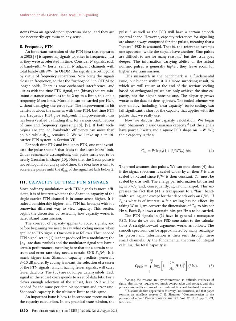
Fig. 2 shows the frequency of error events4 for FTN

with � ¼ 0:5; 0:35; 0:25. These values lie well below the

Mazo limit and represent strong ISI and narrowband

transmission. The base pulse hðtÞ is the 30% rRC pulse.This h has spectrum zero outside 1:3=2T Hz and so the

sequence fvng is in theory infinite, but a good approxima-

tion results when v has length 13, 17, and 27, respectively.

The last FTN runs at density 8 b/Hz-s and has a huge

memory; no variant of the full VA or BCJR is practical with

this ISI. The heavy solid curves are error estimates based

on a minimum distance analysis. Immediately above are

performances of an M-algorithm BCJR (henceforth calledthe M-BCJR). These show that this reduced-search de-

tector can limit the BCJR recursions respectively to 4, 7, 20

fang�!

Linear modulation by hðtÞ at rate1

�T�!AWGN channel�!

Matched filter�! Sample at n�T�!Discrete-time filter BðzÞ�! fyng�!Detect fang: (6)

3Named after its authors Bahl–Cocke–Jelinek–Raviv and published in1974 [17]. BCJR is based on the earlier Baum–Petrie algorithm foridentifying models. The algorithm lay dormant many years, wasrecognized as the critical element in turbo decoding in the early 1990s,and won a paper prize, finally, in 1998.

4Errors in FTN and error-correction decoding do not occur in isolatedbit errors, but rather in multibit events. Error statistics and distanceanalysis relate to these events. Details about the tests and the receiveralgorithm can be found in [11] and [13].



signal paths through the ISI trellis and still achieve near-

optimal performance.5 A reduced-trellis Viterbi decoder of

size 256 and 4096 states is shown for comparison at� ¼ 0:35; 0:25; the 4096 state reduction is much too sev-

ere, but the normal reduced VA is impractical.

It is interesting to observe that the � ¼ 0:25 FTN case

has the same PSD shape as 256-ary QAM modulation with

the same hðtÞ. But 256QAM needs Eb=N0 � 24 dB to

achieve error rate � 10�6, 4–5 dB more than the � ¼ 0:25

plot. The Shannon capacity CPSD crosses the x-axis at about

12 dB. In a similar way, ordinary 16QAM compares to the� ¼ 0:5 case, both having bit density 4 b/Hz-s. Error rate

10�6 is reached at about 15 and 13 dB, respectively, with

CPSD at 4.7 dB. These comparisons show that uncoded

FTN is significantly more energy efficient than QAM at the

same error rate and bandwidth, but that it still lies well

above capacity.

All the � here lie well below the Mazo limit � ¼ 0:703.

With 0.703, 16-state reduced-trellis VA designs existthat perform near the theoretical error probability

Qðffiffiffiffiffiffiffiffiffiffiffiffiffiffiffi2Eb=N0

pÞ for ISI-free transmission. The M-algorithm

BCJR requires only three trellis paths. These are simple

detectors, and they make possible a system with 30% less

bandwidth.

Receivers That Work With Colored Noise: For many years

most of detection theory has been concerned with receiv-ers where the processing in the Detect fang block in (6)

assumes the noise is white. The processing is then more

straightforward, but it may be more for a given BER than

the nonwhite alternatives, and resolving this question is a

present research question. Placing a prefilter either before

or after the Matched filter/Sampler blocks in (6) will ingeneral color the noise. It can also reduce the signal set dmin,

which will damage the bit error rate (BER) performance,

but there can be a complexity reduction for a given BER

and Eb=N0.

Examples of recent research in this sort of colored-

noise receiver are Colavolpe et al. [20], who adapt the

BCJR algorithm to colored fyng, and Dang et al. [21], who

analyze the effects of prefiltering. A much older approachis combined linear Viterbi detection (CLVD), which origi-

nated in [22]–[24]. The rationale behind CLVD is to apply

the filter BðzÞ with taps ½b0; b1; . . . ; bN� to the receiver filter

samples, call them fxng, in order to shorten the memory of

the filtered impulse response fvng � fbng. The shortened

response is referred to as the target impulse response vtar

and is constrained to have finite duration L. The two filters

fbng and fvtarn g are jointly optimized so that

fbng � fxng � vtarn

� � fang þ f�ng:

The noise f�ng here is not necessarily white. Details of this

optimization can be found in [22]–[25]. A trellis detector

follows that operates as if the true impulse response were

vtar and the noise were white. With binary pulses, the

number of states has been found to be reasonable with

some FTN pulses.Since the noise may be colored and vtar does not ex-

actly model the signal convolution, the decoder is mis-

matched with its input signal. This is the classical setting of

mismatched decoding. The concept has emerged as a

powerful tool for analyzing practical FTN systems.

V. CODED FTN AND TURBO DECODING

In the last section, we saw that FTN with low-complexity

receivers improves upon simple modulation with the same

bit density, but performance still lies well short of capacity.

What coded systems are available that reach closer to

CPSD? One that has been fully researched at this writing isa rate R convolutional code driving a binary FTN modula-

tor. Now the fang sequences in (1) are convolutional

codewords, and the data bit density is reduced by a factor

R.6 Standard practice for many years is to place an inter-

leaver before the FTN modulation, so that the receiver can

break up the error bursts that are characteristic of ISI. The

convolutional encoder defines an allowed subset of se-

quences from (1), and we have a true coded system.In principle a maximum-likelihood decoder, perhaps a

VA, could estimate which word from the code was sent. As

a trellis structure, the code would have a state space that

was the product of the convolutional and FTN state spaces.

5The M-algorithm VA will perform a little better in this application.The required trellis decision depth is 15–40, depending on the value of � .

6An equivalent view is that the encoder drives an orthogonalmodulation, which then passes through an ISI channel.

Fig. 2. Error event rates for simple rRC FTN detection versus

Es=N0 in decibels; an M-algorithm BCJR (dotted) is compared

to a reduced-trellis VA (dash–dot) and a distance-based estimate.

(From [11].)



But with convolutionally coded FTN and small � , the VA

would be far too large. A way out of this called turbo

equalization was proposed by Douillard et al. [16] and is

sketched in Fig. 3. The transmitter and the channel are the

traditional convolutional code/interleaver/ISI, but the re-

ceiver is an iterative detector consisting of two soft de-coders in a feedback loop, one for the ISI and one for the

convolutional code. An interleaver and deinterleaver reas-

semble the transmission in the right order, and they also

make the inputs to the soft decoders quasi-independent,

which is essential to proper convergence of the itera-

tions. The soft information needs to flow around the loop

5–50 times, depending on the SNR and the ISI.

The critical elements in the feedback loop are the softdecoders, and the design of these is a major subject. It is

crucial that the information fed around is soft. Instead of

decisions about bits, it must be a statement of their proba-

bilities: in turbo equalization, the log-likelihood ratio

(LLR) is used.7 The standard algorithm to compute soft

information values for signals that can be organized in a

trellis structure is the aforementioned BCJR algorithm.

The algorithm consists of forward and backward linearrecursions that work along the received sequence; there is

no add/compare/select as in the VA. It is still true that the

ISI has a very large trellis structure, and like the VA, the

BCJR needs to be simplified and focused, either by reduc-

ing its trellis or by reducing the regions of the trellis where

it performs calculations. These algorithms are active re-

search areas.

The convolutional encoder can be simple, and mostresearch has in fact studied the memory-2 feedforward

(7, 5) encoder, the standard introductory example in many

textbooks. The best convolutional code depends on the

operating Eb=N0 [19], but its BCJR is in any case small. Theinterleavers, however, need to be long and this sets the

coding scheme’s block length. The overall coded FTN

structure includes the interleaver, as does a turbo code,

and is thus neither simple nor short.

Fig. 4 shows the BER of the (7, 5) 4-state convolutional

code and the � ¼ 1=3 FTN. The BER plot has two

fundamental properties. At some low threshold Eb=N0

(�3.5 dB in the figure), the BER suddenly drops from ahigh value. Thereafter, the data BER tracks that of the

convolutional code over an ISI-free AWGN channel with

the same Eb=N0; this ‘‘CC line’’ appears in the figure. The

ISI–BCJR application in the first iteration is the simple

detection in Section IV, and it produces error rate

� Qðffiffiffiffiffiffiffiffiffiffiffiffiffiffiffiffiffiffiffiffid2

minEs=N0

pÞ. Shown for comparison is a Nyquist-

pulse 64-state TCM system with the same PSD shape and

same 3 b/Hz-s. It has a fixed complexity for all Eb=N0,about the same as the turbo decoder operating at Eb=N0

above 5–6 dB. It depends for its operation on orthogonal

pulses.

When the FTN-induced ISI is this long or longer, the

ISI–BCJR can be replaced by an M-algorithm BCJR [12],

[13]. This greatly reduces computation, and under these

conditions the ISI–BCJR in Fig. 4 can limit its computation

to 5–100 trellis paths and the turbo decoder needs 3–40turbo iterations and block length 1500–40 000, all

depending on how far Eb=N0 lies from capacity. The high

figures will bring BER performance to within 1 dB of

capacity, as shown in the figure.

A special version of the capacity CPSD called the

Shannon BER capacity is shown as a heavy dashed line, for

systems with the 30% rRC PSD that carry 3 b/Hz-s. This

useful curve shows the limit to the BER of any systemworking at the Eb=N0 on the x-axis, for the given PSD and

Fig. 3. Iterative detection of FTN signals. The simple detection in

Section IV includes just the dashed box. P denotes an interleaver.

7Receivers like that in Fig. 3 were studied as early as 1970, but failedbecause they fed around hard bit decisions.

Fig. 4. BERs for Nyquist-pulse TCM and convolutionally coded

� ¼ 1=3 FTN versus Eb=N0 in decibels, at 3 b/Hz-s. All signals have

30% rRC PSD. rRC and sinc pulse capacities for 3 b/Hz-s shown

for comparison. ‘‘CC line’’ denotes (7, 5) code BER over ISI-free

AWGN channel (capacities do not apply to this line).



bit density. We will skip the details of the calculation.8 Thecoded FTN system lies as close as 1 dB to the BER version

of CPSD and the TCM system lies about 2 dB further away.

The lighter dashed curve gives the BER capacity when hðtÞis replaced by the sinc pulse, or alternately, when coding is

limited to Nyquist pulses. This curve is a BER capacity, but

starting from Csq in (4). The curve lies 0.7 dB closer to

both schemes, but it is not the correct reference for the

FTN scheme.The complexity of coded FTN is thus at the ‘‘iterative’’

level. ISI–BCJRs with much reduced complexity have been

developed, and there is much research on turbo decoding

hardware, but even so the total complexity and block

length are not small. Reducing computation and inter-

leaver length, or using a shortened ISI model v easily drive

performance away from Shannon capacity, and diminish

the reward for using iterative detection in the first place.

VI. MORE ON CAPACITY

In Section III, we gave the fundamental capacity integral

for signals that, like FTN, have a certain PSD. Although (5)

states the ultimate information rate for a PSD, the pro-

mised rate can only be achieved under the ideal assump-

tions of Gaussian-distributed data and optimal detection.

This section explores how capacity is affected by practical

constellations of the input values, such as occur in QAM or

PSK, or by processing, such as occurs in the suboptimalCLVD receiver. Aside from being interesting in itself, the

CLVD idea also simplifies capacity calculation, and helps

answer the question of how close coded FTN can come

to CPSD.

For true maximum-likelihood (ML) detection, the

capacity constrained to a certain input constellation is

the highest mutual information, denoted IML, between the

input and output of the channel

IML ¼ max I fyng; fangð Þ: (7)

Here the max is over the probability distributions of y and

a, given AWGN, the FTN ISI and the constellation con-

straint. The long memory of the ISI makes IML difficult to

evaluate, and one way to simplify the problem is to add the

constraint that CLVD processing is present. This shortens

the channel memory, and as a side benefit suggests a

potentially practical low-complexity detector. We denotethe new highest mutual information by ICLVD. It must be

true that CPSD � IML � ICLVD, where the first inequality

holds since the Gaussian input assumption has been re-

laxed and the second holds because ML-detection has been

relaxed. The rate ICLVD is derived in [25], based on the

results of [26] and [27].

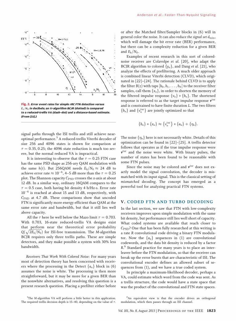
Fig. 5 shows the results of some of these capacity

calculations. We show the max ICLVD, expressed as bits

per second, for optimized CLVD reception for � ¼ 0:5;0:35; 0:25. The memory of the target impulse response L is2, 4, 6, which correspond to a complexity of 4, 16, 64 states

in the model. The three curves marked with circles,

squares, and triangles show the constrained capacities of

the competing Nyquist systems ð� ¼ 1Þ, based on 4ASK

(amplitude shift keying), 8ASK and 16ASK (with complex-

valued constellations, these correspond to 16QAM,

64QAM, 256QAM). The heavy line shows the capacity

of a Nyquist system with random Gaussian-distributedinput values, which is the optimal strategy from a capa-

city point of view. As can be seen, the FTN systems are

always superior to the competing Nyquist systems. In

fact, � ¼ 0:35 and 0:25 FTN outperforms the optimal

Gaussian-based Nyquist system even though it works with

a small fixed set of channel input values and its curve is an

underbound. This has even been shown for binary ASK

with small enough � [14].It may appear that coded FTN violates the Shannon

limit, but this is, of course, not the case. An FTN system

has the ability to exploit the excess bandwidth of the base

pulse hðtÞ. This is not the case for systems based on otho-

gonal pulses, whose performance is independent of the

excess bandwidth in the orthogonal pulse. Some study of

(4) and (5) shows that the dependence of capacity on

8Shannon demonstrated how to compute such curves in 1959; themethod is adapted to coded FTN in [18] and works from (5). In (5), the3-dB bandwidth of the 30% RC jHðfÞj2 is set to 1 Hz and CPSD ¼ 3 b/Hz-s.

Fig. 5. Plot of underbound to achievable rates ICLVD versus P=N0 for

FTN and Nyquist schemes. Circles, squares, and triangles denote M-ary

ASK Nyquist systems with M ¼ 16;64; 256. The heavy solid line uses

Gaussian inputs and marks the ultimate limit of Nyquist transmission.

Curves with no markers denote binary-input FTN systems with

� ¼ 0:5;0:35;0:25, which have the same bits per Hz-s and PSD shape

as the ASK systems. There exist binary FTN systems that outperform

the ultimate Nyquist transmission.



bandwidth is roughly linear, whereas it depends logarith-

mically on power. As P=N0 grows, even a small fraction of

power lying in a PSD stopband has a major effect. There is

no FTN capacity ‘‘bonus’’ with sincðt=TÞ pulses, but as

soon as a practical pulse is substituted for sinc, new capa-

city appears.

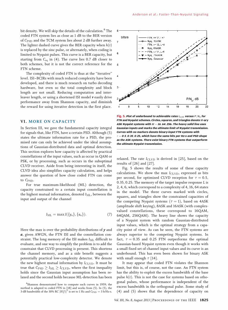
A Carrier Modulation Example: The capacity advantageextends also to carrier modulation systems. Consider the

bit-interleaved coded modulation (BICM) system in Fig. 6,

where QPSK feeds an FTN system with � ¼ 1=2. A se-

quence of bits u feeds two memory-2 shift-register pre-

coders, one of which is preceded by a length-100 000

interleaver (details can be found in [28]). Mapping to

QPSK and FTN modulation follow, and the receiver is an

iterative decoder in the style of Section V. This FTN systemcan be viewed as working with complex-valued data and

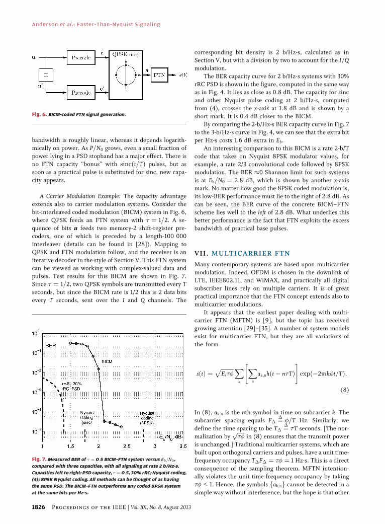
pulses. Test results for this BICM are shown in Fig. 7.

Since � ¼ 1=2, two QPSK symbols are transmitted every Tseconds, but since the BICM rate is 1/2 this is 2 data bits

every T seconds, sent over the I and Q channels. The

corresponding bit density is 2 b/Hz-s, calculated as inSection V, but with a division by two to account for the I=Qmodulation.

The BER capacity curve for 2 b/Hz-s systems with 30%

rRC PSD is shown in the figure, computed in the same way

as in Fig. 4. It lies as close as 0.8 dB. The capacity for sinc

and other Nyquist pulse coding at 2 b/Hz-s, computed

from (4), crosses the x-axis at 1.8 dB and is shown by a

short mark. It is 0.4 dB closer to the BICM.By comparing the 2-b/Hz-s BER capacity curve in Fig. 7

to the 3-b/Hz-s curve in Fig. 4, we can see that the extra bit

per Hz-s costs 1.6 dB extra in Eb.

An interesting comparison to this BICM is a rate 2-b/T

code that takes on Nyquist 8PSK modulator values, for

example, a rate 2/3 convolutional code followed by 8PSK

modulation. The BER �0 Shannon limit for such systems

is at Eb=N0 ¼ 2.8 dB, which is shown by another x-axismark. No matter how good the 8PSK coded modulation is,

its low-BER performance must lie to the right of 2.8 dB. As

can be seen, the BER curve of the concrete BICM–FTN

scheme lies well to the left of 2.8 dB. What underlies this

better performance is the fact that FTN exploits the excess

bandwidth of practical base pulses.

VII. MULTICARRIER FTN

Many contemporary systems are based upon multicarrier

modulation. Indeed, OFDM is chosen in the downlink ofLTE, IEEE802.11, and WiMAX, and practically all digital

subscriber lines rely on multiple carriers. It is of great

practical importance that the FTN concept extends also to

multicarrier modulations.

It appears that the earliest paper dealing with multi-

carrier FTN (MFTN) is [9], but the topic has received

growing attention [29]–[35]. A number of system models

exist for multicarrier FTN, but they are all variations ofthe form

sðtÞ ¼ffiffiffiffiffiffiffiffiffiEs��

p Xk

Xn

ak;nhðt� n�TÞ" #

exp �2�ik�t=Tð Þ:

(8)

In (8), ak;n is the nth symbol in time on subcarrier k. The

subcarrier spacing equals F� ¼� �=T Hz. Similarly, we

define the time spacing to be T� ¼��T seconds. [The nor-

malization byffiffiffiffiffi��p

in (8) ensures that the transmit poweris unchanged.] Traditional multicarrier systems, which are

built upon orthogonal carriers and pulses, have a unit time-

frequency occupancy T�F� ¼ �� ¼ 1 Hz-s. This is a direct

consequence of the sampling theorem. MFTN intention-

ally violates the unit time-frequency occupancy by taking

�� G 1. Hence, the symbols fak;ng cannot be detected in a

simple way without interference, but the hope is that other

Fig. 6. BICM-coded FTN signal generation.

Fig. 7. Measured BER of � ¼ 0:5 BICM–FTN system versus Eb=N0,

compared with three capacities, with all signaling at rate 2 b/Hz-s.

Capacities left to right: PSD capacity, � ¼ 0:5, 30% rRC; Nyquist coding,

(4); 8PSK Nyquist coding. All methods can be thought of as having

the same PSD. The BICM–FTN outperforms any coded 8PSK system

at the same bits per Hz-s.



gains can be harvested at the expense of receiver com-

plexity. Fig. 8 imagines the fak;ng (crosses) superposed on

the time-frequency locations of the original orthogonal

transmission (dots), and shows how one pulse can inter-fere with its neighbors in frequency and time.9 When �� is

near 1, the interference will be mostly with nearest neigh-

bors, but lower �� will lead to much more interference and

to a challenging detection problem.

An alternate description of these signals appears in [42].

The Mazo limit extends naturally to MFTN. There is a

smallest product T�F� such that the minimum distance

remains at the matched filter bound. With QPSK inputsand a 30% rRC pulse, the smallest product reported where

there is no loss in minimum distance is near 0.5 [9], which

corresponds to a doubling of the spectral efficiency.

Unfortunately, the state space associated with trellis

detection of MFTN is far larger than for single-carrier

FTN. This fact has motivated research in applicable low-

complexity detection [30], [31]. In [29], a memoryless de-

tector for FTN is investigated. Such a detector has thesame order of complexity as a detector for orthogonal sys-

tems, regardless of the product T�F�. More precisely, the

detector works as follows. Suppose that we want to decode

the nth symbol in time on the kth subcarrier. Then, a

decision variable can be formed by the inner product

rk;n ¼R1�1 rðtÞ �k;ndt, where rðtÞ is the received signal and

k;n is an arbitrary function (� denotes complex conju-

gate). In [29], k;n is chosen as the matched filter k;n ¼h�ðt� n�T�Þ expð2�iktF�Þ, but other functions such as an

minimum mean square error (MMSE) filter can be used.

The decision variable can be broken into a signal-dependent part, an interference-dependent part, and a

noise part, in the form

rk;n ¼ffiffiffiffiEs

pak;n þ

X‘ 6¼k;m 6¼n

�‘;ma‘;m|fflfflfflfflfflfflfflfflfflffl{zfflfflfflfflfflfflfflfflfflffl}Interference

þ �k;n: (9)

Finally, the interference term is modeled as Gaussian noise

so that the received signal model becomes

rk;n ¼ffiffiffiffiEs

pak;n þ ~�k;n: (10)

The variance of ~�k;n is higher than N0=2 due to the inter-

ference and ~H is not white, but the model is the same as

that of an interference-free system and its complexity does

not depend on T�F�. Spectral efficiency grows with de-creasing T�F�, but at the same time the receiver perfor-

mance deteriorates. According to [29], a good compromise

lies near �� ¼ 0:8.

A Coded MFTN Receiver: We conclude this section with

a test of a coded MFTN system that has 50 carriers � 100

QPSK symbols, together with an outer (7, 5) convolutional

code. We use the same system model as Fig. 3, but the‘‘ISI’’ box is replaced by an MFTN modulator. The mem-

oryless detector described above has been used, in com-

bination with soft interference cancellation. In each

iteration, soft estimates of the interference terms f�‘;mgin (9) are calculated based on the LLRs from the channel

decoder. The estimates are then subtracted from rk;n be-

fore the a posteriori LLRs are calculated. Interleaver size

10 000 b and seven iterations were used, although manyfewer are required for products 0.5 and 0.55. The results

for the products �� ¼ 0:45; 0:5; 0:55 appear in Fig. 9;

� ¼ 0:8 always, so that � ¼ 0:5626; 0:625; 0:6875. All

three cases show BER similar to the no-ISI convolutional

code at high SNR, but the spectral efficiency is roughly

doubled.

Without FTN, the bit density here is only 1 b/Hz-s; the

time-frequency MFTN roughly doubles this spectralefficiency to 1=��, or about 2. The BICM system in

Fig. 7 has the same spectral efficiency in terms of 3-dB

power bandwidth and is much more energy efficient, but it

requires a far more complex receiver.

VIII . HARDWARE IMPLEMENTATIONS

A main reason that FTN-like communication is not yet in

wide use is its computational complexity. The situation can

be compared to LDPC codes that needed some 40 years

from their initial proposal by Gallager in 1963 to their

Fig. 8. Time-frequency view of multicarrier FTN, showing ISI and

intercarrier interference (ICI) paths. For simplicity, only time

squeezing is employed in this example. (Courtesy D. Dasalukunte,

Lund University, Lund, Sweden.)

9For simplicity, Fig. 8 takes the original orthogonal frequencyspacing. In reality, the new subcarriers lie closer and are phase shifts ofeach other; the shift is a design parameter in the FTN system.



hardware implementation in the 21st century. Bandwidth

efficiency cannot after all be achieved by introducing a

computational overhead that consumes most of the bene-

fits. Hardware for FTN signaling began to appear around

2009, when integrated circuits matured enough to copewith the complexity demands. Tradeoffs have to be made

between energy and bandwidth performance on the one

hand and hardware complexity on the other. From a prac-

tical perspective, it is also important that FTN systems

utilize hardware resources that are similar to those in

conventional systems.

The first FTN hardware implementation papers [36]–

[38] mainly investigated complexity issues related to thetransmitter. Due to their popularity, multicarrier systems

have been the primary focus, and one issue has been how

FTN-based signaling can be combined with a traditional

OFDM system without wasting resources. References [37],

[38] investigate a hardware transmitter architecture based

on lookup tables that projects the FTN symbols onto an

orthogonal basis function set (represented, for example, by

the dots in Fig. 8). IOTA pulses10 are used to reduce theprojections onto neighboring pulses. Since IOTA filters

are already used to help remove the cyclic prefix of

OFDM systems, this is an attractive solution. Another

group at the University College London (London, U.K.)

has proposed an implementation based on several phase-

shifted inverse fast Fourier transforms (IFFTs), whose

signals are combined to form frequency compressed FTN

signals [40]–[42]. These works studied transmitters only

and were mainly verified by field-programmable gate

array (FPGA)-based implementations.

The major challenges in FTN hardware implementa-tion are associated with the receiver. As the product ��drops well below one and compression increases, hard-

ware complexity, memory requirements, and energy con-

sumption grow rapidly in a receiver that has near-ML error

performance. With time-frequency FTN, the processing is

a 2-D exchange between time and frequency detectors.

Reception becomes very complex in the region 0:5 G�� G 0:7, even though it lies above the Mazo limit, and thesearch for efficient detection algorithms has only just

begun in this region. Still, good receivers are a worthwhile

goal because they offer large bandwidth compaction with

little loss in BER.

To our knowledge, the first hardware architecture

implemented in silicon for an FTN receiver based on

multicarrier modulation was presented in [43]–[45]. The

T�F� was kept as an adjustable parameter, i.e., in a badchannel with strong ISI, the system can back off to tradi-

tional OFDM, while in a good channel, compression can be

high. Fig. 10 gives a block diagram of the transceiver. A

complete iterative decoder based on the successive inter-

ference cancellation in the last section is implemented in

hardware. The system includes an outer convolutional

code, and a max-log-MAP BCJR convolutional decoder in

the receiver. Several hardware optimization techniqueswere employed to lower the complexity without severely

damaging the receiver performance. The architecture was

implemented in 65-nm complementary metal–oxide–

semiconductor (CMOS) and occupied 0.8 mm2; clock

speed was 100 MHz and power consumption was 9.6 mW

at supply voltage 1.2 V. Up to 16 turbo iterations can be

executed and T�F� is selectable over f0:4; 0:5; 0:6;0:7; 0:9g. At eight iterations, the data throughput was1 Mb/s. This early work shows that the complexity intro-

duced by FTN signaling can be handled in modern silicon

10The isotropic orthogonal transform algorithm (IOTA) pulse is anorthogonalization of the Gaussian pulse that is isotropic in time and fre-quency. They thus reduce the total spread of ISI and ICI. See [39] and [46].

Fig. 10. Block diagram of FTN coded transmitter/receiver

implemented in hardware in [43]. (Courtesy D. Dasalukunte,

Lund University.)Fig. 9. Simulation of (7, 5) encoded MFTN systems with different

products TDFD and memoryless SIC detection of the MFTN system.

‘‘CC line’’ denotes (7, 5) reference performance with orthogonal

signaling. All three MFTN systems converge toward the reference.

Interleaver size 10 000 b and seven iterations.



processes. Further hardware implementations of FTNsystems seem just around the corner.

IX. CONCLUSION

FTN signaling, either coded or uncoded, can provide up to

twice the bandwidth efficiency of ordinary modulation

without consuming more transmitter energy per bit. Below

a threshold called the Mazo limit, more energy is needed,but the signaling still offers attractive combinations of

bandwidth and energy efficiency, which allow operation in

new regions of the energy–bandwidth plane. We have

demonstrated these facts with tests of a number of

software implementations of both baseband and carrier

systems. One explanation for this better performance is

that unlike Nyquist-pulse signaling, FTN takes advantage

of the higher Shannon information rate that practical pulsetransmission makes available. At the same time, FTN is a

direct extension of techniques such as QAM and OFDM

that are already in place. New FTN hardware chips thattake advantage of this have already begun to appear.

As higher bit rate wireless systems grow in impor-

tance and become shorter range, they gain SNR and need

to carry more data bits in the same spectrum. The same

can be said for single-carrier systems such as satellite

digital television, which find themselves with more SNR

but still must work in the same radio-frequency (RF)

channel. We have quantified the idea of more bits perunit of bandwidth by introducing the concept of bit

density. New systems need to operate at densities of

3–8 b/Hz-s, rather than the lower values that have

applied until now. These densities are available with

uncoded large-alphabet QAM modulation, but fewer

options are known for coded systems. As a general tech-

nique coding offers energy and bandwidth gains at high

densities as well as low, and it is precisely in the relativelyunexplored high densities that coded FTN offers new

possibilities. h

RE FERENCES

[1] J. E. Mazo, ‘‘Faster-than-Nyquist signaling,’’Bell Syst. Tech. J., vol. 54, pp. 1451–1462,Oct. 1975.

[2] C.-K. Wang and L.-S. Lee, ‘‘Practicallyrealizable digital transmission significantlybelow the Nyquist bandwidth,’’ in Proc. IEEEGlobal Commun. Conf., Phoenix, AZ, USA,Dec. 1991, pp. 1187–1191.

[3] N. Seshadri, ‘‘Error performance of trellismodulation codes on channels with severeintersymbol interference,’’ Ph.D. dissertation,Dept. Electr., Comput. Syst. Eng., RensselaerPolytechnical Inst., Troy, NY, USA,Sep. 1986.

[4] A. D. Liveris and C. N. Georghiades,‘‘Exploiting faster-than-Nyquist signaling,’’IEEE Trans. Commun., vol. 51, no. 9,pp. 1502–1511, Sep. 2003.

[5] P. Kabal and S. Pasupathy, ‘‘Partialresponse signaling,’’ IEEE Trans. Commun.,vol. COMM-23, no. 9, pp. 921–934,Sep. 1975.

[6] A. Said and J. B. Anderson,‘‘Bandwidth-efficient coded modulationwith optimized linear partial-responsesignals,’’ IEEE Trans. Inf. Theory,vol. 44, no. 2, pp. 701–713, Mar. 1998.

[7] J. B. Anderson and A. Svensson, CodedModulation Systems. New York, NY,USA: Kluwer/Plenum, 2003.

[8] F. Rusek and J. B. Anderson, ‘‘The twodimensional Mazo limit,’’ in Proc. IEEEInt. Symp. Inf. Theory, Adelaide, Australia,Sep. 2005, pp. 970–974.

[9] F. Rusek and J. B. Anderson, ‘‘Multi-streamfaster than Nyquist signaling,’’ IEEE Trans.Commun., vol. 57, no. 5, pp. 1329–1340,May 2009.

[10] F. Rusek and J. B. Anderson, ‘‘Optimalsidelobes under linear and faster thanNyquist modulation,’’ in Proc. IEEE Int.Symp. Inf. Theory, Nice, France, Jun. 2007,pp. 2301–2304.

[11] J. B. Anderson, A. Prlja, and F. Rusek,‘‘New reduced state space BCJR algorithmsfor the ISI channel,’’ in Proc. IEEE Int.Symp. Inf. Theory, Seoul, Korea, Jun. 2009,pp. 889–893.

[12] J. B. Anderson and A. Prlja, ‘‘Turboequalization and an M-BCJR algorithmfor strongly narrowband intersymbolinterference,’’ in Proc. Int. Symp. Inf.Theory Appl., Taichung, Taiwan, Oct. 2010,pp. 261–266.

[13] A. Prlja and J. B. Anderson,‘‘Reduced-complexity receivers forstrongly narrowband intersymbol interferenceintroduced by faster-than-Nyquist signaling,’’IEEE Trans. Commun., vol. 60, no. 9,pp. 2591–2601, Sep. 2012.

[14] Y. G. Yoo and J. H. Cho, ‘‘Asymptoticoptimality of binary faster-than-Nyquistsignaling,’’ IEEE Commun. Lett.,vol. 14, no. 9, pp. 788–790, Sep. 2010.

[15] F. Rusek and J. B. Anderson, ‘‘Constrainedcapacities for faster than Nyquist signaling,’’IEEE Trans. Inf. Theory, vol. 55, no. 2,pp. 764–775, Feb. 2009.

[16] C. Douillard, A. Picart, P. Didier, M. Jezequel,C. Berrou, and A. Glavieux, ‘‘Iterativecorrection of intersymbol interference: Turboequalization,’’ Eur. Trans. Telecommun.,vol. 6, pp. 507–511, Sep./Oct. 1995.

[17] L. R. Bahl, J. Cocke, F. Jelinek, and J. Raviv,‘‘Optimal decoding of linear codes forminimizing symbol error rate,’’ IEEE Trans.Inf. Theory, vol. IT-20, no. 2, pp. 284–287,Mar. 1974.

[18] J. B. Anderson and F. Rusek, ‘‘The Shannonbit error limit for linear coded modulation,’’ inProc. Int. Symp. Inf. Theory Appl., Parma, Italy,Oct. 2004, pp. 9–11.

[19] J. B. Anderson and M. Zeinali, ‘‘Best rate1/2 convolutional codes for turbo equalizationwith severe ISI,’’ in Proc. IEEE Int. Symp.Inf. Theory, Cambridge, MA, USA, Jul. 2012,pp. 2366–2370.

[20] G. Colavolpe and A. Barbieri, ‘‘On MAPsymbol detection for ISI channels usingthe Ungerboeck observation model,’’ IEEECommun. Lett., vol. 9, no. 8, pp. 720–722,Aug. 2005.

[21] U. L. Dang, W. H. Gerstacker, andS. T. M. Slock, ‘‘Maximum SINR prefilteringfor reduced-state trellis-based equalization,’’in Proc. IEEE Int. Conf. Commun., Kyoto,Japan, Jun. 2011, DOI: 10.1109/icc.2011.5963034.

[22] D. D. Falconer and F. R. Magee, ‘‘Adaptivechannel memory truncation for maximumlikelihood sequence estimation,’’ BellSys. Tech. J., vol. 52, pp. 1541–1562,Nov. 1973.

[23] S. A. Fredricsson, ‘‘Joint optimization oftransmitter and receiver filter in digitalPAM systems with a Viterbi detector,’’IEEE Trans. Inf. Theory, vol. IT-22, no. 2,pp. 200–210, Mar. 1976.

[24] C. T. Beare, ‘‘The choice of the desiredimpulse response in combined linear-Viterbialgorithm equalizers,’’ IEEE Trans. Commun.,vol. COMM-26, no. 8, pp. 1301–1307,Aug. 1978.

[25] F. Rusek and A. Prlja, ‘‘Optimal channelshortening of MIMO and ISI channels,’’IEEE Trans. Wireless Commun., vol. 11, no. 2,pp. 810–818, Feb. 2012.

[26] N. Merhav, G. Kaplan, A. Lapidoth, andS. Shamai Shitz, ‘‘On information ratesfor mismatched decoders,’’ IEEE Trans.Inf. Theory, vol. 46, no. 6, pp. 1953–1967,Nov. 1994.

[27] A. Ganti, A. Lapidoth, and I. E. Telatar,‘‘Mismatched decoding revisited: Generalalphabets, channels with memory, andthe wide-band limit,’’ IEEE Trans. Inf.Theory, vol. 46, no. 6, pp. 2315–2328,Nov. 2000.

[28] F. Rusek and J. B. Anderson, ‘‘Serial andparallel concatenations based on fasterthan Nyquist signaling,’’ in Proc. IEEEInt. Symp. Inf. Theory, Seattle, WA, USA,Jul. 2006, pp. 1993–1997.

[29] A. Barbieri, D. Fertonani, and G. Colavolpe,‘‘Time-frequency packing for linearmodulations: Spectral efficiency andpractical detection schemes,’’ IEEE Trans.Commun., vol. 57, no. 10, pp. 2951–2959,Oct. 2009.

[30] I. Kanaras, ‘‘Spectrally efficient multicarriercommunication systems: Signal detection,mathematical modelling and optimisation,’’Ph.D. dissertation, Dept. Electron. Electr.Eng., Univ. College London, London, U.K.,2010.

[31] A. Chorti, I. Kanaras, M. R. D. Rodrigues, andI. Darwazeh, ‘‘Joint channel equalizationand detection of spectrally efficient FDMsignals,’’ in Proc. IEEE Conf. Pers. Indoor



Mobile Radio Commun., Istanbul, Turkey,Sep. 2010, pp. 177–182.

[32] S. Isam and I. Darwazeh, ‘‘Precoded spectrallyefficient FDM system,’’ in Proc. IEEE Conf.Pers. Indoor Mobile Radio Commun., Istanbul,Turkey, Sep. 2010, pp. 99–104.

[33] I. Kanaras, A. Chorti, M. Rodrigues, andI. Darwazeh, ‘‘Investigation of a semidefiniteprogramming detection for a spectrallyefficient FDM system,’’ in Proc. IEEE Conf.Pers. Indoor Mobile Radio Commun., Tokyo,Japan, Sep. 2009, pp. 2827–2832.

[34] M. He, D. Liang, and Q. Cao, ‘‘A modulationwith higher bandwidth efficiency thanOFDM,’’ in Proc. Int. Conf. Signal Process.Syst., Dalian, China, Jul. 2010, pp. 393–397.

[35] F.-M. Han and X.-D. Zhang, ‘‘Wirelessmulticarrier digital transmission viaWeyl-Heisenberg frames over time-frequencydispersive channels,’’ IEEE Trans. Commun.,vol. 57, no. 6, pp. 1721–1733, Jun. 2009.

[36] I. Kanaras, A. Chorti, M. R. D. Rodrigues, andI. Darwazeh, ‘‘Spectrally efficient FDMsignals: Bandwidth gain at the expense ofreceiver complexity,’’ in Proc. IEEE Int. Conf.Commun., Dresden, Germany, Jun. 2009,DOI: 10.1109/ICC.2009.5199477.

[37] D. Dasalukunte, F. Rusek, J. B. Anderson, andV. Owall, ‘‘A transmitter architecture forfaster-than-Nyquist signaling systems,’’ inProc. IEEE Int. Symp. Circuits Syst., Taipei,Taiwan, May 2009, pp. 1028–1031.

[38] D. Dasalukunte, F. Rusek, V. Owall,K. Ananthanarayanan, and M. Kandasamy,‘‘Hardware implementation of mapper forfaster-than-Nyquist signaling transmitter,’’ inProc. IEEE NORCHIP, Trondheim, Norway,Nov. 2009, DOI: 10.1109/NORCHP.2009.5397801.

[39] B. Le Floch, M. Alard, and C. Berrou,‘‘Coded orthogonal frequency divisionmultiplex,’’ Proc. IEEE, vol. 83, no. 6,pp. 982–996, Jun. 1995.

[40] M. R. Perrett and I. Darwazeh, ‘‘Flexiblehardware architecture of SEFDM transmitterswith real-time non-orthogonal adjustment,’’ inProc. 18th Int. Conf. Telecommun., Cyprus,May 2011, pp. 369–374.

[41] P. N. Whatmough, M. R. Perrett, S. Isam, andI. Darwazeh, ‘‘VLSI architecture for areconfigurable spectrally efficient FDMbaseband transmitter,’’ in Proc. IEEE Int.Symp. Circuits Syst., Rio de Janeiro, Brasil,May 2011, pp. 1688–1691.

[42] P. N. Whatmough, M. R. Perrett, S. Isam,and I. Darwazeh, ‘‘VLSI architecture fora reconfigurable spectrally efficient FDMbaseband transmitter,’’ IEEE Trans. CircuitsSyst. I, Reg. Papers, vol. 59, no. 5,pp. 1107–1118, May 2012.

[43] D. Dasalukunte, F. Rusek, and V. Owall,‘‘Multicarrier faster-than-Nyquist signalingtransceivers: Hardware architecture andperformance analysis,’’ IEEE Trans.Circuits Syst. I, Reg. Papers, vol. 58, no. 4,pp. 827–838, Apr. 2011.

[44] D. Dasalukunte, F. Rusek, and V. Owall,‘‘Improved memory architecture formulticarrier faster-than-Nyquist iterativedecoder,’’ in Proc. IEEE Comput. Soc. Annu.Symp. Very Large Scale Integr., Chennai, India,Jul. 2011, pp. 296–300.

[45] D. Dasalukunte, F. Rusek, and V. Owall,‘‘A 0.8 mm2 9.6 mW implementation of amulticarrier faster-than-Nyquist signalingiterative decoder in 65 nm CMOS,’’ in Proc.38th Eur. Solid State Circuits Conf., Bordeaux,France, Sep. 2012, pp. 173–176.

[46] M. Alard, ‘‘Construction of a multicarriersignal,’’ U.S. Patent 6 278 686, Aug. 2001.

ABOUT THE AUT HORS

John B. Anderson (Fellow, IEEE) was born in

New York State in 1945. He received the Ph.D.

degree in electrical engineering from Cornell

University, Ithaca, NY, USA, in 1972.

During 1972–1980, he was on the electrical

engineering faculty at McMaster University,

Hamilton, ON, Canada, and during 1981–1998, he

was a Professor at Rensselaer Polytechnic Insti-

tute, Troy, NY, USA. Since 1998, he has held the

Ericsson Chair in Digital Communication at Lund

University, Lund, Sweden. He has held visiting professorships at the

University of California at Berkeley (Berkeley, CA, USA), Chalmers Univ-

ersity (Goteborg, Sweden), Queen’s University (Kingston, ON, Canada),

Deutsche Luft und Raumfahrt (Cologne, Germany), and Technical Univ-

ersity of Munich (Munich, Germany). He was the Director of the Swedish

Strategic Research Foundation Center for High Speed Wireless Commu-

nication at Lund University during 2005–2011. He is an author of six

textbooks, including most recently Digital Transmission Engineering

(Piscataway, NJ, USA: IEEE Press, 2005, 2nd ed.), Coded Modulation Sys-

tems (New York, NY, USA: Plenum/Springer, 2003), and Understanding

Information Transmission (Piscataway, NJ, USA: IEEE Press, 2005). Since

1998, he has edited the IEEE Press book Series on Digital and Mobile

Communication. His research work is in coding and communication

algorithms, bandwidth-efficient coding, and the application of these to

data transmission and compression. He has served widely as a consultant

in these fields.

Dr. Anderson was a member of the IEEE Information Theory Society

Board of Governors during 1980–1987 and 2001–2006, serving as the

Society’s Vice President and President (1985). In 1983 and 2006, he was

Co-Chair of the IEEE International Symposium on Information Theory. In

the IEEE publications sphere, he served on the Publications Board of the

IEEE on three occasions, and was Editor-in-Chief of IEEE PRESS during

1994–1996 and 2012–2014. He has also served as an Associate Editor for

several IEEE TRANSACTIONS. He received the Humboldt Research Prize

(Germany) in 1991. In 1996, he was elected Swedish National Visiting

Chair in Information Technology. He received the IEEE Third Millennium

Medal in 2000.

Fredrik Rusek was born in Lund, Sweden, in 1978.

He received the M.S. and Ph.D. degrees in electri-

cal engineering from Lund University, Lund,

Sweden, in 2003 and 2007, respectively.

Since 2008, he has held an assistant profes-

sorship at the Department of Electrical and Infor-

mation Technology, Lund University. His research

interests include modulation theory, equalization,

wireless communications, and applied informa-

tion theory.

Viktor Owall (Member, IEEE) received the M.Sc.

and Ph.D. degrees in electrical engineering from

Lund University, Lund, Sweden, in 1988 and 1994,

respectively.

During 1995–1996, he joined the Electrical

Engineering Department, University of California

at Los Angeles, Los Angeles, CA, USA, as a Post-

doctoral Researcher, where he mainly worked in

the field of multimedia simulations. Since 1996, he

has been with the Department of Electrical and

Information Technology, Lund University. He is currently full Professor at

the same department and since 2009 the Head of the Department. He

is the Director of the VINNOVA Industrial Excellence Center in System

Design on Silicon (SoS). His main research interest is in the field of

digital hardware implementation, especially algorithms and architec-

tures for wireless communication, image processing, and biomedical

applications. His research projects include combining theoretical

research with hardware implementation aspects in the areas of wireless

communication, video processing, and digital holography.

Dr. Owall was an Associate Editor of the IEEE TRANSACTIONS ON CIRCUITS

AND SYSTEMSVPART II: ANALOG AND DIGITAL SIGNAL PROCESSING from 2000 to

2002 and of the IEEE TRANSACTIONS ON CIRCUITS AND SYSTEMSVPART I:

REGULAR PAPERS from 2007 to 2009. He was Guest Editor for the Special

issue on ISCAS 2010 of the IEEE TRANSACTIONS ON BIOMEDICAL CIRCUITS AND

SYSTEMS.



Documents

INVITED PAPER Faster-Than-NyquistSignaling called faster-than-Nyquist (FTN) signaling. Its roots trace back to the 1970s, but it has attracted inter-est in our bandwidth-starved world