INVITED PAPER CapacityTrends andLimitsofOptical ... · INVITED PAPER CapacityTrends andLimitsofOptical CommunicationNetworks ... fiber nonlinear optics; ... we present an overview

INV ITEDP A P E R

Capacity Trendsand Limits of OpticalCommunication NetworksDiscussed in this paper are: optical communication network traffic evolution trends,

required capacity and challenges to reaching it, and basic limits to capacity.

By Rene-Jean Essiambre, Senior Member IEEE, and Robert W. Tkach, Fellow IEEE

ABSTRACT | Since the first deployments of fiber-optic com-

munication systems three decades ago, the capacity carried by

a single-mode optical fiber has increased by a staggering

10 000 times. Most of the growth occurred in the first two

decades with growth slowing to ten times in the last decade.

Over the same three decades, network traffic has increased by

a much smaller factor of 100, but with most of the growth

occurring in the last few years, when data started dominating

network traffic. At the current growth rate, the next factor of

100 in network traffic growth will occur within a decade. The

large difference in growth rates between the delivered fiber

capacity and the traffic demand is expected to create a capacity

shortage within a decade. The first part of the paper recounts

the history of traffic and capacity growth and extrapolations for

the future. The second part looks into the technological chal-

lenges of growing the capacity of single-mode fibers by pre-

senting a capacity limit estimate of standard and advanced

single-mode optical fibers. The third part presents elementary

capacity considerations for transmission over multiple trans-

mission modes and how it compares to a single-mode trans-

mission. Finally, the last part of the paper discusses fibers

supporting multiple spatial modes, including multimode and

multicore fibers, and the role of digital processing techniques.

Spatial multiplexing in fibers is expected to enable system

capacity growth to match traffic growth in the next decades.

KEYWORDS | Channel capacity; communication system traffic;

fiber nonlinear optics; multiple-input–multiple-output (MIMO);

optical fiber communication; optical networks

I . INTRODUCTION

Optical communications is unchallenged for the transmis-

sion of large amounts of data over long distances with low

latency and it underlies modern communications net-

works, in particular the internet. The transmission capa-

city of optical network technology has made dramatic

strides over the decades since its introduction in the early

1970s. The early years of optical communications werecharacterized by a steady development of technology, a

moderate rate of increase of bit rate in the single optical

channel supported on these systems and the gradual

change of the optical frequency transmission windows

from 800 to 1300 to 1550 nm [1]–[3]. The latter part of the

1990s saw dramatic increases in system capacity brought

about through the use of wavelength division multiplexing

(WDM) enabled by optical amplifiers. This technologicalrevolution ignited massive investment in system develop-

ment both from traditional vendors as well as new en-

trants, and the capacity of commercial lightwave systems

increased from less than 100 Mb/s when they debuted in

the 1970s to roughly 1 Tb/s by 2000 [4]. This is an increase

of more than 10 000 times in 30 years, but more incre-

dibly, the introduction of WDM resulted in a factor of

1000 increase in just 10 years. This was enabled by thesimple addition of more wavelengths to systems which

were not limited by the available optical bandwidth. In the

last decade, progress has slowed dramatically since the

readily available bandwidth has become occupied and in-

creases in capacity now require improvements in the effi-

ciency of the utilization of optical bandwidth. The rapid

growth in system capacity catalyzed by WDM resulted in

system capacities that exceeded the requirements of net-work traffic for most of the past decade. However, the

continued rapid growth of traffic has reversed this situa-

tion and now the need for increased system capacity is

Manuscript received August 19, 2011; revised December 12, 2011; accepted

December 22, 2011. Date of publication March 16, 2012; date of current version

April 18, 2012.

The authors are with Bell Laboratories, Alcatel-Lucent, Holmdel, NJ 07733 USA

(e-mail: [email protected]; [email protected]).

Digital Object Identifier: 10.1109/JPROC.2012.2182970

Vol. 100, No. 5, May 2012 | Proceedings of the IEEE 10350018-9219/$31.00 �2012 IEEE

becoming acute. The current trends of traffic growth andsystem capacity increase will result in system capacity

falling behind traffic by a factor of 10 over the next decade.

Scaling system capacity to meet this challenge will be

difficult and will require breakthroughs on a similar scale

to the introduction of large-scale wavelength division

multiplexing. This growth in traffic coupled with observed

trends in commercial practice will also result in a re-

quirement for interfaces to the core network to migratefrom the current 10, 40, and 100 Gb/s to 1 Tb/s by 2020.

Terabit single-channel bit rates seem extremely difficult to

achieve by pursuing current technological paths.

In this paper, we present an overview of the challenges

associated to the rapid growth of traffic demand and of the

slower growth in network capacity. We evaluate a maxi-

mum fiber capacity estimate for a wide variety of single-

mode fibers and discuss possible capacity scaling throughspatial multiplexing in fibers and associated new fiber

technologies.

II . NETWORK TRAFFIC

Internet traffic has been growing strongly since the earliest

days of personal computers. At various times different

applications have been cited as the drivers of this growth,

but an examination of growth rates shows a fairly steady

growth rate over the last 15 years [5].1 Fig. 1 shows North

American Internet traffic data from various sources over

the period from 1990 through the present and some fore-casts through 2015. There are two sources for the traffic

data: the Minnesota Internet Traffic Study (MINTS) [6]

and a report from the Discovery Institute by Swanson and

Gilder [7]. The MINTS data shows a period of rapid growth

in 1996, but the remainder of the years show a growth rate

ranging from 100% a year in the early years to 50% to 60%a year since 2000. The latest growth rate estimate from

this data is 50% to 60% a year as of year-end 2008. The

Swanson and Gilder data shows very good agreement with

the MINTS data. The other set of points on the chart are

from a forecast prepared by Cisco in 2007 [8] and revised

in 2011 [9]. The 2007 forecast is consistent with the 2008

data from MINTS and predicts a similar growth rate until

2011, while the 2011 revision suggests a slightly reducedgrowth rate. While the current estimated growth rates are

far less than the Bdoubling every 100 days[ sometimes

quoted in the late 1990s through 2000 [10], they still give

rise to an increase in traffic by a factor of 100 in 10 years.

The solid line on Fig. 1 is set at the mean of the high and

low estimates for 2007 and extrapolated using the esti-

mated growth rate for year-end 2008. It is clear that the

growth rate has been fairly consistent since 2000. Whilethere are a variety of services that underlie the traffic de-

mand described above it is possible to see a reason for the

traffic growth that is independent of the individual services

but instead considers trends in the technology used to

support those services. In particular, it is useful to look at

the evolution of microprocessor speed and data storage.

The Top 500 organization charts the performance increase

of the 500 fastest supercomputers and has shown an in-crease of 10 times in 4 years since the early 1990s [11].

Individual microprocessors have shown a similar improve-

ment rate. Since the data traffic we are interested in ori-

ginates and terminates on machines made up of these

processors, it is unsurprising that the traffic scales at es-

sentially the same rate. Alternatively traffic can be thought

of as movement of data. The International Data Corpora-

tion (IDC) has estimated the total amount of stored data toincrease by a factor of 10 in 5 years again essentially equal

to the rate of traffic increase [12]. Both the speed of the

devices connected to the network and the total amount of

information stored are scaling at the same rate we observe

for network traffic and these underlying trends show no

sign of abating.

III . SYSTEM CAPACITY

Optical communications underwent a revolution in the

1990s as optical amplifiers and WDM enabled the informa-

tion carried on a single fiber to move from a few gigabits

per second to over one terabit per second. This rapid ex-

pansion of system capacity is visible in Fig. 2. The points

on the figure are total capacities for a single fiber in

laboratory/research demonstrations. Points are also dis-tinguished by whether WDM is employed. Generally, only

points which represent a new record of capacity are

plotted. Various time periods exhibit relatively stable

growth rates with relatively sharp demarcations between

them. We see an initial rapid rise in capacity for single-

channel time division multiplexing (TDM) demonstrations

as researchers employed available microwave components

1Some of the material in this section and the next has been presentedin an earlier form in [5] but is updated and expanded here.

Fig. 1. North American Internet traffic.

Essiambre and Tkach: Capacity Trends and Limits of Optical Communication Networks

1036 Proceedings of the IEEE | Vol. 100, No. 5, May 2012

in digital circuits. Progress levels-off in the late 1980s as

the optical system speed became limited by the speed of

components and further progress was controlled by therate of technological development of transistors. Another

rapid rise in capacity begins in 1993 when the availability

of optical amplifiers, dispersion management, and gain

equalization enabled the application of WDM. The availa-

ble spectrum was rapidly populated by more channels until

1996, when the spectrum was nearly filled, and the first

1 Tb/s experiments were being performed [13]–[15]. From

this time until the present, a slower rate of capacity in-crease is observed as research focused on increased spec-

tral efficiency (SE). Fig. 3 shows the SE achieved in these

demonstrations as a function of year. It is clear from the

figure that improvements in SE have driven the im-

provements in capacity. The current capacity record of

101.7 Tb/s achieved a SE of 11 b/s/Hz [16] (see Fig. 9)

using coherent detection, offline processing and pilot-

tone-based phase-noise mitigation. The modulation format

is quadrature amplitude modulation (QAM) with 128 con-

stellation points (128-QAM) [17]. The signal-to-noise ratio

required for this format, combined with the limitationsimposed by impairments arising from optical fiber nonlin-

earity, allowed transmission over only three relatively

short, Raman-amplified spans. The SE of this result is im-

pressive and it is worth noting that improving it by a factor

of two via a more complex constellation would require the

use of 16 384-QAM and would increase the required opti-

cal signal-to-noise ratio (OSNR) by about two orders of

magnitude making transmission over useful distances im-possible given the presence of nonlinear effects in fibers

described in Section IV. Fig. 4 shows the capacity of com-

mercial optical communication systems as a function of the

year of introduction. These tend to track the research de-

monstrations of Fig. 3 with a three to seven year delay. The

point at 8.8 Tb/s in late 2009 corresponds to a system with

88 100-Gb/s channels using polarization-multiplexed

QPSK modulation and coherent detection. The solid linesin Fig. 4 provide a continuous representation of system

capacity vs. year and are projected into the future. The

slope of the line from 2000 forward corresponds to a

growth rate of less than 20% per year. The curve in Fig. 4

is the composite network traffic composed of the data

traffic extrapolation described above combined with voice

traffic which dominated the network before 2002 but

grows slowly. Notice that the total network traffic andsystem capacity cross twice. First, in 2000, commercial

system capacity increases through the total network traffic

and it became possible to buy a system that could carry the

entire network traffic on a single fiber pair. Second, the

Fig. 2. Demonstrated system capacities. Single channel TDM

systems (filled circles) WDM systems (filled squares).

Fig. 3. Spectral efficiency achieved in research demonstrations

versus year.

Fig. 4. Commercial system capacities (squares) and total network

traffic including voice (blue curve) using measurements and

projections from Fig. 1 and measured and projected voice traffic

as of 1998.


Vol. 100, No. 5, May 2012 | Proceedings of the IEEE 1037

two curves cross again in 2008, when traffic growth re-sulted in network traffic exceeding system capacity. In the

following years the projected curves diverge with traffic

outstripping capacity by more than a factor of 10 per

decade.

It is important to note that there is no obvious reason

to compare network traffic with the capacity of a single

optical communication system; however, the comparison

can be justified, at least when plotted on a logarithmicaxis. The capacity of a link must obviously be larger than

the traffic carried on that link; typically the factor is

between two and five, accounting for peak to average

traffic ratios [18]. Of course, the traffic on a link is not the

same as the traffic in the network. In North America there

are three to five links passing east to west, so we might

expect that link traffic would be roughly three to five

times lower than network traffic. These two errors are inopposing directions and one may hope that the compar-

ison carries at least qualitative and order-of-magnitude

value.

As system capacity scales to meet the growth of net-

work traffic, it is important for the speed of interface rates

to the networking equipment to increase as well in order

to limit the increase in complexity of the network. Fig. 5

shows interface rates for a variety of networking equip-ment plotted against the year of commercial introduction.

The plot starts with an early high-speed interface at

168 Mb/s [19], [20] through today. The years before

2000 are characterized by a variety of rates for various

layers of the network, with cross connects and internet

protocol (IP) routers using lower rates than those available

for transmission. In 2000, we see a remarkable coalescing

of rates at 10 Gb/s for transmission, cross connects, androuters. While this plot overstates the case, since inter-

faces introduced in earlier years persist in the network, it

is clear that there has been a substantial flattening of thenetwork; the utility of low bit rate circuits and the network

elements that provision them becomes marginal as inter-

face rates to nodal equipment rise. The line on the graph is

drawn through the transmission points and attempts to

project the evolution of interface rates into the next

decade. This extrapolation suggests that 1-Tb/s interfaces

will be used towards the end of the decade. The slope of

the line is roughly a factor of 10 in 10 yearsVsimilar to thatseen for the extrapolation of system capacity. Thus far we

have only examined trends and extrapolated their contin-

uation. Now we turn our attention to the requirements

that these trends in traffic and capacity will place on sys-

tem design. We begin by reviewing the evolution of some

key system parameters. The earliest WDM systems had

between four and eight 2.5-Gb/s channels and were intro-

duced in 1995 [2]. These first systems had capacities on theorder of 20 Gb/s and operated on a 200-GHz channel

spacing resulting in a SE of 0.0125 b/s/Hz. By 2000,

systems had rapidly advanced to 80 or more 10-Gb/s chan-

nels operating on 50-GHz spacing for capacities of nearly

1 Tb/s, and a SE of 0.2 b/s/Hz. Commercial systems

introduced in 2010 operate with 100-Gb/s channels on

50-GHz spacing with SE of 2.0 b/s/Hz. To obtain the

same factor of 10 improvement over the next decadewould imply systems with 1-Tb/s channels, capacity of

100 Tb/s, and SE of 20 b/s/Hz. Clearly these are very

challenging specifications. In fact, further increase in

capacity will be hampered by significant limitations arising

from fiber nonlinearity as we see below.

IV. LIMITS TO SYSTEM CAPACITY

As shown in Fig. 2, there has been a tremendous increase

in capacity of three orders of magnitude in the last two

decades. Clearly, it is of interest to investigate whether

there are fundamental limits to this capacity increase. In

this section, we first briefly review Shannon’s information

theory for the additive white Gaussian noise (AWGN)channel and then present results of calculations of a

Bnonlinear Shannon limit[ associated to the presence of

the Kerr nonlinear effects in fibers.

A. Shannon CapacityThe notion of Bcapacity[ of a channel was introduced

in 1948 by Claude Shannon [22].2 The capacity of a chan-

nel can be described as the asymptote of the rates oftransmission of information that can be achieved with

arbitrarily low error rate. In his seminal work [22],

Shannon focused primarily on a channel that adds white

Gaussian noise, and more specifically, the AWGN channel

[23]–[25]. In the last 60 years, Shannon’s Binformation

Fig. 5. Interface rates for a variety of networking equipment versus

year of introduction. Optical communication systems (squares),

cross connects (diamonds), and IP routers (triangles).

2A channel in the sense of Shannon is not to be confused with aWDM channel in optical communication, which is a signal occupying acertain frequency band, often contaminated by noise and other sources ofdistortion.



theory[ has been applied and adapted to more complexchannels such as wireless communication [26]–[33], digi-

tal subscriber lines (DSLs) over twisted copper wires [34]–

[38], coaxial cables [36]–[39] and the Bphoton channel[[40]–[45], relevant to deep space and satellite commu-

nications [46], [47].

We review in this section the capacity relations for a

single-channel with AWGN that we later use as a reference

in the multiple channels Section V-A. For a bandlimitedchannel, it is convenient3 to quote the SE defined as the

capacity C per unit of bandwidth B. From Shannon’s

theory, the SE of a single AWGN channel is given by the

well-known relation [23], [25]

SE � C

B¼ log2ð1þ SNRÞ (1)

where the signal-to-noise ratio SNR is defined as SNR ¼P=N where P is the signal average power and N the noise

average power in a bandwidth B. We consider here a

signal constructed from a serial concatenation of symbols

at a rate of Rs symbols per seconds. Many bits of infor-

mation can be encoded using the amplitude and phase ofthe signal on each symbol. The minimum bandwidth that

such a signal can have while remaining free from

intersymbol interference (ISI) [48], [49] at the optimum

sampling point is equal to the value of the symbol rate Rs

[22], [50]–[52]. This signal is generated using a field

waveform of the form sinðtÞ=t associated with each

symbol [17], [48]. For such a minimum-bandwidth signal,

the noise power N ¼ N0Rs, where N0 is the noise powerspectral density. The SNR can be written as [30], [31],

[48], [49]

SNR � P

N¼ P

N0Rs¼ Es

N0(2)

where the last equality is obtained using the relation

P ¼ EsRs, where Es is the energy per symbol. Note that

both, signal and noise, are represented by complex fields,

each having two quadratures. At low SNR, (1) can be

approximated by

SE � 1

ln 2SNR� SNR2

2

� �: (3)

An interesting observation from (3) is that both SE andSNR, or Es at fixed N0, go to zero simultaneously, i.e.,

one cannot achieve high SE at low SNR on a single

channel.

Using (2) one can define an SNR per bit, SNRb, as [25],

[48], [49]

Eb

N0� SNRb ¼

SNR

SE(4)

where the energy per bit Eb ¼ Es=SE. The SNR per bit

can therefore be interpreted as the energy per bit per unit

of noise power spectral density. Equation (1) can bereexpressed as

SNRb ¼2SE � 1

SE: (5)

The SNR per bit can be written as SNRb ¼ Eb=N0 where

Eb ¼ Es=SE is the energy per bit. At high SE, SNRb �2SE=SE.

One can write (5) as a series expansion around SE ¼ 0.

It is given by SNRb ¼PQ

q¼0ðln 2Þqþ1SEq=ðqþ 1Þ!. Expan-

sion to second order and at low SE gives

SNRb � ln 2þ ðln 2Þ2

2SE þ ðln 2Þ3

6SE2: (6)

One notes that, in contrast to the relation between

SE and SNR of (3), the SNR per bit, SNRb, does not go

to zero when SE goes to zero, but assumes a minimum

value

SNRminb ¼ ln 2 (7)

or � �1:59 dB [53] (see Fig. 6). There is, therefore, a

minimum SNR or energy per bit to transmit information

over the AWGN channel [23], [25] and this minimum

occurs at low SNR.

It is interesting to define the ratio �SNRb

�SNRb � SNRb=SNRminb (8)

which can be referred to as an excess SNR or energy per bit

at which a system operates. The quantity �SNRb, in dB, is

represented schematically on the Shannon curve of Fig. 6,

3For simplicity, we use the word capacity to refer to either capacity orSE in this paper as both are simply related by the channel bandwidth B.



which also shows the approximation to first and second

order in SE from (6).We can also express the SE as a function of SNRb to

first order in SNRb as

SE � 2

ðln 2Þ2SNRb � SNRmin

b

� �: (9)

B. Relations between SNR and OSNRIn optical communication, the optical signal-to-noise

ratio is the quantity typically reported to characterize the

ratio between signal and noise. In other areas of digital

communication, the SNR is used. The quantities involved

in both OSNR and SNR definitions are displayed in Fig. 7.The OSNR is written as

OSNR ¼ P

2NASEBref(10)

where P is the average signal power, summed over the

two states of polarization if polarization division multi-

plexing (PDM) is used, NASE is the spectral density of

amplified spontaneous emission per polarization and Bref

is a reference bandwidth, commonly taken to be 0.1 nm,

which corresponds to 12.5 GHz at 1550 nm. Note that

the definition of OSNR does not require the signal to

carry any data since the OSNR definition uses a fixedreference bandwidth Bref instead of the symbol rate Rs

used in the SNR definition [see (2)]. The OSNR also

considers the noise in both polarization states indepen-

dent of whether PDM of the signal is used or not. From(2) and (10), the relation between OSNR and SNR can be

expressed as

OSNR ¼ pRs

2BrefSNR (11)

where p ¼ 1 for a singly-polarized signal and p ¼ 2 for a

PDM signal, and where NASE and N0 have canceled each

other out since they represent the same physical quantity,

the noise power spectral density [17].

Equation (12) can also be written in the following

form

OSNR ¼ Rs

BrefSNRð2Þ (12)

Fig. 7. Definition of signal and noise for the (a) signal-to-noise ratio (SNR) and (b) optical signal-to-noise ratio (OSNR). l.u.: linear units.

Fig. 6. Spectral efficiency versus SNR per bit for a single channel,

a few approximations of SNRb and a graphic representation

of DSNRb.



where SNRð2Þ is the average SNR over the two polarizationmodes. It is defined as

SNRð2Þ �Px þ Py

Nx þ Ny(13)

where the indices x and y refer to the x and y polarizations,

respectively. In this definition of SNRð2Þ, when the signal

is singly-polarized, the signal power originates from one

polarization while the noise power remains summed over

both polarizations. This definition of SNR has the advan-tage that it can easily be generalized to a large number of

modes [see (21)].

We define the information bit rate RðpÞb , in bits per

second, as the sum of the information rates in both polari-

zation states. Assuming the same structure of the signal for

both polarizations if PDM is used, i.e., same symbol rate

Rs, same number of constellation points per polarization

M, and same code rate ~Rc, the bit rate RðpÞb , valid for a

singly-polarized or a PDM signal, can be written as

RðpÞb ¼ p ~Rc log2ðMÞRs (14)

where ~Rc is the encoder rate, which represents the ratio of

input to output bits at the encoder so that 0 G ~Rc � 1. Notethat the transmission information rate in bits per symbol~R ¼ ~Rc log2ðMÞ can be identified to the SE in Shannon’s

formula (1) for an ideal code and a Gaussian constellation.

For PDM, a symbol corresponding to the symbol rate Rs

extends to both polarization states and represents all the

possible ways to combine the M symbol(s) of each

polarization. The symbol size at the symbol rate Rs is

therefore Mp with p ¼ 2. One can see that (14) can bewritten in a more natural form as R

ðpÞb ¼ ~Rc log2ðMpÞRs,

where log2ðMpÞ represents the number of uncoded bits of

the constellation at Rs. Using (4), one can express (12) as

OSNR ¼ RðpÞb

2BrefSNRb (15)

where SNRb is the SNR per bit in one of the polarization

state having a signal.

Note that the relation between OSNR and SNRb

requires only the knowledge of RðpÞb , but does not require to

know whether the signal is singly-polarized or if PDM is

used. Equation (15) can be also expressed as

OSNR ¼ RðpÞb

pBrefSNR

ð2Þb (16)

where SNRð2Þb ¼ pSNRb=2 is the SNR per bit accounting

for the two polarization modes.

C. Nonlinear Shannon Limit for a NonlinearFiber Channel

It is only relatively recently that information theoretic

approaches have been applied to fiber-optic communica-

tion systems based on single-mode fibers (SMFs) [17],

[54]–[79] (more details can be found in [17]). This Flate_focus on the Bfiber channel[ is mainly due to the fact that

an optical fiber is a Kerr nonlinear medium [80]–[83],

which raises many challenges. One of them is that there is

no well established framework of information theory to

calculate the capacity of a channel that is simultaneously

nonlinear and bandwidth-limited. A second difficulty is

the absence of closed-form analytic expressions describing

fiber propagation for arbitrary input signal shapes andpower levels.

Capacity limitations of the most commonly studied

channels originate from the presence of in-band sources of

distortion, being either in-band noise or some form of in-

band interference coming from other sources [30], [31],

[84]. The capacity of these channels typically increases

monotonically with power. In the case of the nonlinear

fiber channel, the capacity is limited by noise at low powerbut becomes limited by fiber nonlinearity as power in-

creases. Remarkably, in the context of optically-routed

networks (ORNs), the high-power fiber capacity limita-

tions originate mainly from fields present outside the

bandwidth of the signal of interest [17] and lead to a

maximum capacity. Fig. 8 illustrates schematically the

nonlinear process that results in capacity limitation for the

nonlinear fiber channel. The presence in a fiber of a WDMchannel occupying a distinct frequency band from a WDM

channel of interest, changes the refractive index of the

fiber medium through the Kerr nonlinear effect [85]. Since

Fig. 8. Schematic illustration of the main nonlinear process limiting

capacity in fiber.



the WDM channel of interest is also present in the fiber, it

experiences these variations of refractive index and be-

comes distorted. In general, the change of refractive index

depends not only on power but also on the data being

transmitted [86]–[88]. Since different WDM frequency

bands are optically routed to different physical locations in

optical networks, the data of the copropagating WDM

channels are not known and distortions created by copro-pagating WDM channels on the WDM channel of interest

cannot be fully compensated [17].

Nonlinear propagation through optical fibers is de-

scribed by the partial differential equation [17]

@E

@zþ i

2�2@2E

@t2� i�jEj2E ¼ iN (17)

where Eðz; tÞ is the optical field at a given location z and

time t, �2 is the fiber chromatic dispersion, � the fiber

nonlinear coefficient and Nðz; tÞ is the field that repre-

sents amplified spontaneous emission (ASE). The field

Eðz; tÞ is assumed to be singly polarized and (17) is written

for a system using ideal distributed Raman amplificationwhere the Raman gain continuously compensates for fiber

loss [89]. The fiber nonlinear coefficient � ¼ n2!s=ðcAeffÞwhere n2 is the fiber nonlinear refractive index [83],

!s ¼ 2��s is the angular optical frequency at the signal

wavelength with �s being the optical carrier frequency,

c the speed of light and Aeff the fiber effective area [83].

Assuming that ASE generated by optical amplification

can be represented by an AWGN source [90], [91],Shannon’s information theory can therefore be applied to

evaluate the impact of ASE noise on capacity. The autocor-

relation [92] of the ASE field Nðz; tÞ is given by [93]–[95]

E N ðz; tÞN �ðz0; t0Þ½ � ¼ �Lh�sKT�ðz� z0Þ�ðt� t0Þ (18)

where E½� is the expectation value operator and � the Dirac

functional. The factor KT ¼ 1þ �ðT; �s; �pÞ where

�ðT; �s; �pÞ is the phonon occupancy factor [17], [96],

[97]. The value of KT � 1:13 at room temperature.

For ideal distributed Raman amplification, the noise

spectral density per state of polarization can be written

as [53], [89]

NASE ¼ �Lh�sKT (19)

where L is the system length and h the Planck constant.

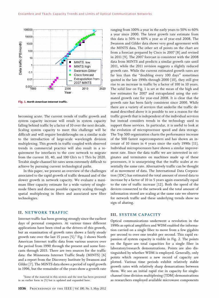
The noise power per polarization is simply NASERs.The capacity calculation of the nonlinear fiber channel

in the context of ORNs has been performed under certain

assumptions summarized in Table 1. Fiber capacities are

computed for a single WDM channel of interest in an

ORN, assuming that all other WDM channels are simul-

taneously present, but not known at the transmitter or

receiver. The constellations adopted are concentric ring

constellations that approach closely the Shannon capacityeven though a small gap from Shannon curves that can be

seen at SNR | 25 dB in Fig. 9 still remains. Routing in

the network is performed using optical filters approaching

the ideal square shape and is performed sufficiently

frequently (every 100 km) that more frequent use of

optical filters does not impact capacity. The signal is

recovered by first performing ideal coherent detection

followed by digital signal processing using reverse

Table 1 Assumptions in the Model to Calculate a Fiber Capacity Estimate

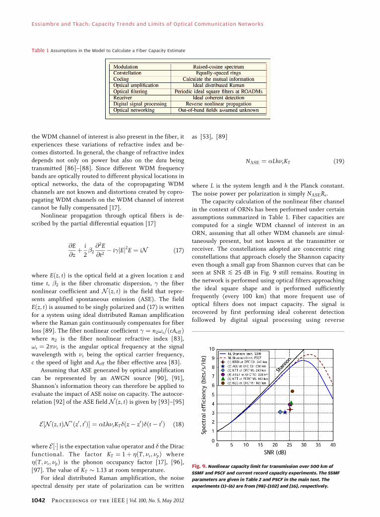
Fig. 9. Nonlinear capacity limit for transmission over 500 km of

SSMF and PSCF and current record capacity experiments. The SSMF

parameters are given in Table 2 and PSCF in the main text. The

experiments (1)–(6) are from [98]–[102] and [16], respectively.



nonlinear propagation performed on the fields present in

the frequency band of the WDM channel of interest.

Because of the various approximations made during theevaluation of capacity, we refer to these nonlinear fiber

capacities as estimates. Extensive explanations on how the

nonlinear fiber capacity calculations have been performed

can be found in [17], [70].

D. Standard Single-Mode FiberThe parameters of the standard single-mode fiber

(SSMF) are given in Table 2 and the corresponding non-

linear capacity estimate is given in Fig. 9. The six filledsymbols in Fig. 9 represent the latest record SE experi-

ments (from 2009 to August 2011) that propagate over at

least 100 km. Also shown are the calculated nonlinear

capacity estimates when the loss coefficient � ¼0:15 dB/km and the effective area Aeff ¼ 120 m2, param-

eters achievable for pure silica-core fibers (PSCFs). The

experimental results are within a factor 1.6 to 3 from the

estimated capacity. Note that the highest SE experimentshave been achieved for distances shorter than 500 km and

that a reduction in SE is expected if the distance were to be

extended to 500 km.

Calculations of nonlinear fiber capacity estimates have

been performed for various distances and the results are

displayed in Fig. 10. One observes that the SNR at which

the capacity peaks decreases by �2.65 dB for every doubl-

ing of the distance. Since the ASE noise power increases by

3 dB when the distance doubles, the optimum signal power

has a weak dependence on distance, decreasing by only

1.4 dB for the range of distance of 500 to 8000 km. One

can understand this surprising result by realizing that

higher capacities are achieved using denser constellations

(largerM), and that the larger the constellation, the moresensitive a signal is to nonlinear distortions. These larger

constellations prevent raising the signal power signifi-

cantly, even when the transmission distance is shortened

dramatically. Note that having a nearly distance-indepen-

dent optimum signal power is advantageous in network

designs, since optical amplifiers can operate at nearly the

same power per WDM channel for a wide range of

distances.Fig. 11 shows the maximum SE values for each curve in

Fig. 10. These calculated SE values fit well a linear relation

when the distance is plotted in a logarithmic scale, so a

linear fit to the SE is also shown in Fig. 11.

The types of networks covered by the various distances

of the plot are shown near the bottom. As can be seen in

the figure, the maximum SE of submarine (SM), ultra-

long-haul (ULH), and long-haul (LH) does not vary widelyconsidering that the range of distances covered is more

than one order of magnitude. The maximum SE increases

as the distance decreases to metropolitan (metro) and

access networks. Finally, fiber-to-the-home (FTTH) has

the highest maximum SE, but, remarkably, only 3 times

the maximum SE of SM systems. This is a rather small

increase in maximum SE considering that there is a

difference of four orders of magnitude in distancebetween these two types of networks. This illustrates

the difficulty of increasing SE in optical networks based

on SMFs.Fig. 10. Nonlinear capacity curves for a range of transmission

distances.

Fig. 11. Spectral efficiency as a function of distance from data at

maximum capacity of Fig. 10. A linear fit to the data is also provided

along with the type of networks it can be applied to.

Table 2 Standard Single-Mode Fiber Parameters



E. Advanced Single-Mode FibersFor a given optical networking scenario and optical

amplification scheme, the nonlinear fiber capacity de-

pends mainly on the fiber parameters and system length.

We show below the calculated maximum nonlinear fiber

capacity estimates when varying three fiber parameters:

the fiber loss coefficient �, the fiber nonlinear coefficient

�, and fiber dispersion D.

1) Fiber Loss: Fig. 12 shows the dependence of the

maximum nonlinear fiber capacity on the fiber loss

coefficient �dB, which relates to � of (17) by �dB ¼10 log10ðeÞ�. One observes that the maximum nonlinear

capacity does not increase dramatically with a large

reduction of �dB. For instance, reducing �dB from 0.2

to 0.05 dB/km increases capacity only from �8 to

�9 b/s/Hz. It is worth pointing out, however, that adecrease in fiber loss coefficient, which generally occurs at

all wavelengths simultaneously, benefits greatly practical

system deployments by either increasing the distance be-

tween amplification sites or by reducing the Raman pump

power requirements.

It is interesting to note that the dependence of the

maximum capacity on the fiber loss coefficient is nearly

linear when �dB is plotted on a log scale as seen in Fig. 12.Shown on the graph are SSMF typical fiber loss coefficient,

the lowest fiber loss coefficient of 0.1484 dB/km achieved

using PSCF [103], and conjectured 0.05 dB/km that may

possibly be achievable for a hollow-core fiber (HCF) ope-

rating at 2 m [104]. One can see in Fig. 12 that even

though it represents a tremendous challenge to reduce the

fiber loss coefficient below 0.15 dB/km, the benefit on

capacity is surprisingly limited.It is worth pointing out that the benefit of reducing the

fiber loss coefficient will increase for systems not using

ideal distributed Raman amplification, and especially for

systems using discrete amplification based on erbium-

doped fiber amplifiers (EDFAs) [105], [106]. The reason is

that, in ideal distributed Raman amplification systems, the

quantity of noise at the end of the system is proportional to�, while it is approximately proportional to expð�Þ in

systems based on EDFAs [17, eq. (54)].

2) Fiber Nonlinear Coefficient: The fiber nonlinear coef-

ficient can be made to vary by a change of the fiber mate-

rial itself, material properties or through advances in fiber

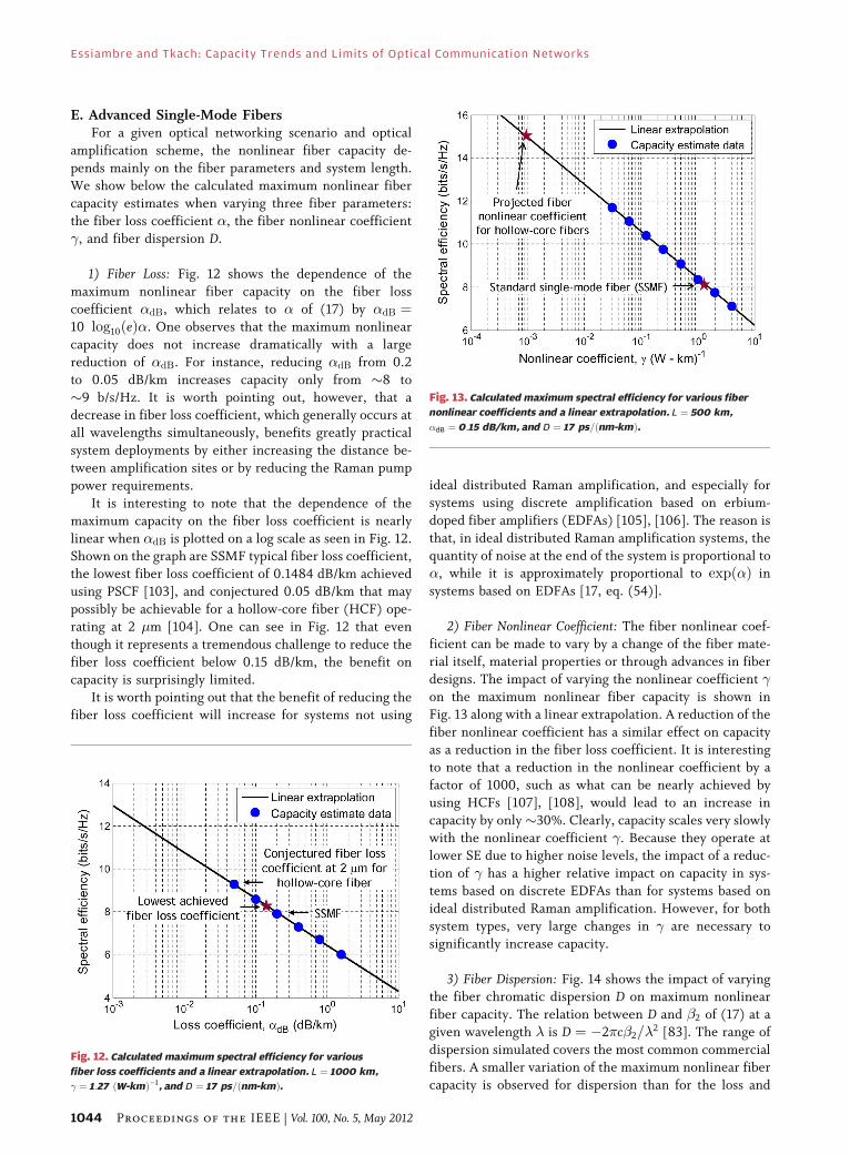
designs. The impact of varying the nonlinear coefficient �on the maximum nonlinear fiber capacity is shown inFig. 13 along with a linear extrapolation. A reduction of the

fiber nonlinear coefficient has a similar effect on capacity

as a reduction in the fiber loss coefficient. It is interesting

to note that a reduction in the nonlinear coefficient by a

factor of 1000, such as what can be nearly achieved by

using HCFs [107], [108], would lead to an increase in

capacity by only�30%. Clearly, capacity scales very slowly

with the nonlinear coefficient �. Because they operate atlower SE due to higher noise levels, the impact of a reduc-

tion of � has a higher relative impact on capacity in sys-

tems based on discrete EDFAs than for systems based on

ideal distributed Raman amplification. However, for both

system types, very large changes in � are necessary to

significantly increase capacity.

3) Fiber Dispersion: Fig. 14 shows the impact of varyingthe fiber chromatic dispersion D on maximum nonlinear

fiber capacity. The relation between D and �2 of (17) at a

given wavelength is D ¼ �2�c�2=2 [83]. The range of

dispersion simulated covers the most common commercial

fibers. A smaller variation of the maximum nonlinear fiber

capacity is observed for dispersion than for the loss and

Fig. 12. Calculated maximum spectral efficiency for various

fiber loss coefficients and a linear extrapolation. L ¼ 1000 km,

� ¼ 1:27 ðW-kmÞ�1, and D ¼ 17 ps=ðnm-kmÞ.

Fig. 13. Calculated maximum spectral efficiency for various fiber

nonlinear coefficients and a linear extrapolation. L ¼ 500 km,

�dB ¼ 0:15 dB/km, and D ¼ 17 ps=ðnm-kmÞ.



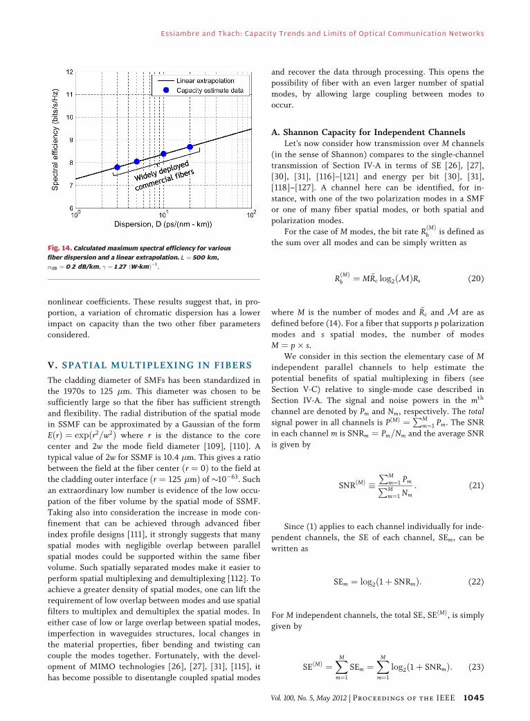
nonlinear coefficients. These results suggest that, in pro-

portion, a variation of chromatic dispersion has a lower

impact on capacity than the two other fiber parameters

considered.

V. SPATIAL MULTIPLEXING IN FIBERS

The cladding diameter of SMFs has been standardized in

the 1970s to 125 m. This diameter was chosen to be

sufficiently large so that the fiber has sufficient strength

and flexibility. The radial distribution of the spatial mode

in SSMF can be approximated by a Gaussian of the formEðrÞ ¼ expðr2=w2Þ where r is the distance to the core

center and 2w the mode field diameter [109], [110]. A

typical value of 2w for SSMF is 10.4 m. This gives a ratio

between the field at the fiber center ðr ¼ 0Þ to the field at

the cladding outer interface ðr ¼ 125 mÞ of�10�63. Such

an extraordinary low number is evidence of the low occu-

pation of the fiber volume by the spatial mode of SSMF.

Taking also into consideration the increase in mode con-finement that can be achieved through advanced fiber

index profile designs [111], it strongly suggests that many

spatial modes with negligible overlap between parallel

spatial modes could be supported within the same fiber

volume. Such spatially separated modes make it easier to

perform spatial multiplexing and demultiplexing [112]. To

achieve a greater density of spatial modes, one can lift the

requirement of low overlap between modes and use spatialfilters to multiplex and demultiplex the spatial modes. In

either case of low or large overlap between spatial modes,

imperfection in waveguides structures, local changes in

the material properties, fiber bending and twisting can

couple the modes together. Fortunately, with the devel-

opment of MIMO technologies [26], [27], [31], [115], it

has become possible to disentangle coupled spatial modes

and recover the data through processing. This opens thepossibility of fiber with an even larger number of spatial

modes, by allowing large coupling between modes to

occur.

A. Shannon Capacity for Independent ChannelsLet’s now consider how transmission over M channels

(in the sense of Shannon) compares to the single-channel

transmission of Section IV-A in terms of SE [26], [27],

[30], [31], [116]–[121] and energy per bit [30], [31],

[118]–[127]. A channel here can be identified, for in-

stance, with one of the two polarization modes in a SMFor one of many fiber spatial modes, or both spatial and

polarization modes.

For the case of M modes, the bit rate RðMÞb is defined as

the sum over all modes and can be simply written as

RðMÞb ¼ M ~Rc log2ðMÞRs (20)

where M is the number of modes and ~Rc and M are as

defined before (14). For a fiber that supports p polarization

modes and s spatial modes, the number of modesM ¼ p s.

We consider in this section the elementary case of Mindependent parallel channels to help estimate the

potential benefits of spatial multiplexing in fibers (see

Section V-C) relative to single-mode case described in

Section IV-A. The signal and noise powers in the mth

channel are denoted by Pm and Nm, respectively. The totalsignal power in all channels is PðMÞ ¼

PMm¼1 Pm. The SNR

in each channel m is SNRm ¼ Pm=Nm and the average SNR

is given by

SNRðMÞ �PM

m¼1 PmPMm¼1 Nm

: (21)

Since (1) applies to each channel individually for inde-

pendent channels, the SE of each channel, SEm, can bewritten as

SEm ¼ log2ð1þ SNRmÞ: (22)

For M independent channels, the total SE, SEðMÞ, is simplygiven by

SEðMÞ ¼XM

m¼1

SEm ¼XM

m¼1

log2ð1þ SNRmÞ: (23)

Fig. 14. Calculated maximum spectral efficiency for various

fiber dispersion and a linear extrapolation. L ¼ 500 km,

�dB ¼ 0:2 dB/km, � ¼ 1:27 ðW-kmÞ�1.



Interesting relations can be obtained when SNRm � 1for all the M channels, where SEðMÞ in (23) simplifies to

SEðMÞ � 1

ln 2

XM

m¼1

SNRm ¼1

ln 2

XM

m¼1

Pm

Nm: (24)

If we further assume that the noise present in all channels

is identical to the noise produced in the reference single

channel, which is a realistic first-order approximation for

spatial multiplexing in fibers, i.e., Nm ¼ N for all values of m,

SEðMÞ simplifies to

SEðMÞ � 1

ln 2

XM

m¼1

Pm

N¼ PðMÞ

N ln 2: (25)

Note that, in this regime of low SNR per channel, SE

depends, to first order, only on the total signal power and

not on the exact distribution of powers between

channels.Let’s now consider systems for which all M channels

have the same SNRm that is not necessarily small: the total

SE of the M channels, SEðMÞ, is simply M times the SE of

each channel. If further, the signal powers in each of the Mchannels identical, i.e., Pm ¼ Pc and similarly all the noise

powers are equal, i.e., Nm ¼ N, SEðMÞ can be written

simply as

SEðMÞ ¼M log2 1þ Pc

N

� �(26)

¼M log2ð1þ �SNRÞ (27)

where SNR ¼ P=N is the SNR in the reference single

channel and � is the ratio of the power in each channel Pc

to P. The reason to express SEðMÞ in terms of the ratio Pc=Pis that, in fibers, Pc and P have maximum values

determined by fiber nonlinearity and fiber types. In the

limit of an infinite number of channels M with a fixed

Pc ¼ P=M, SEð1Þ ! SNR= ln 2, identical to the single-

channel result of (3) to first order in SNR.It is interesting to evaluate the gain in SE

GSE �SEðMÞ

SE(28)

for various values of SNR and signal powers. Restricting

ourselves to channels with identical noise per channel

Nm ¼ N and identical signal power Pc in all channels, onecan write GSE as

GSE ¼M log2ð1þ �SNRÞ

log2ð1þ SNRÞ : (29)

From (29), one can see that three independent parameters

affect GSE: the number of channels M, the ratio of powers

� ¼ Pc=P and the SNR of the reference channel P=N. From(29), when the power per channel Pc equals the single-

channel power P, GSE ¼ M, as it should be for M inde-

pendent channels. Also, when both Pc � N and P� N,

GSE � MPc=P, i.e., the SE increases approximately by the

ratio Pc=P above the value of M when the signal powers are

below the noise power. The power per mode Pc that can be

used for spatial multiplexing in fibers will depend on fiber

nonlinearity and the design of the fiber used for spatialmultiplexing (see Section V-C).

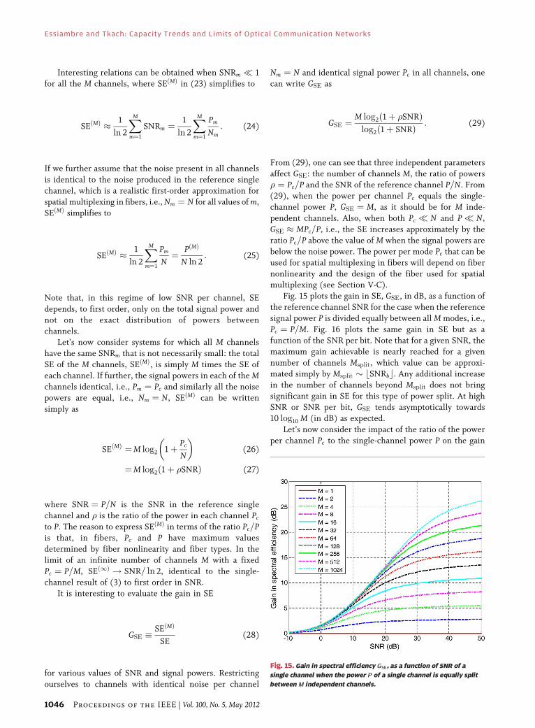
Fig. 15 plots the gain in SE, GSE, in dB, as a function of

the reference channel SNR for the case when the reference

signal power P is divided equally between all M modes, i.e.,

Pc ¼ P=M. Fig. 16 plots the same gain in SE but as a

function of the SNR per bit. Note that for a given SNR, the

maximum gain achievable is nearly reached for a given

number of channels Msplit, which value can be approxi-mated simply by Msplit � bSNRbc. Any additional increase

in the number of channels beyond Msplit does not bring

significant gain in SE for this type of power split. At high

SNR or SNR per bit, GSE tends asymptotically towards

10 log10 M (in dB) as expected.

Let’s now consider the impact of the ratio of the power

per channel Pc to the single-channel power P on the gain

Fig. 15. Gain in spectral efficiency GSE, as a function of SNR of a

single channel when the power P of a single channel is equally split

between M independent channels.



in SE. The ratio Pc=P is a relevant quantity that will bedetermined by the nonlinear effects present in fibers

supporting multiple spatial modes. The impact on trans-

mission of the various nonlinear effects is expected to

depend greatly on fiber designs. From (29), one can see

that the gain in SE per mode, GSE=M, is a quantity

independent of M. Fig. 17 shows the gain in SE per mode as

a function of the ratio Pc=P for various values of SNR. A

negative gain means a reduction in SE. As seen in Fig. 17,the highest values of SNR are the least affected by a

reduction or increase in signal power per channel Pc relative

to the single channel power P. This can be understood by the

fact that a reduction of a few dBs in power when operating at

high SNR on the SE curve changes the SE by only a small

amount relative to the original SE, thereby producing lowergain or loss in SE. Note that this behavior is valid for an

arbitrary number of channels M and that the curves for the

gain in SE alone, GSE, are identical to the curves in Fig. 17 but

shifted up by 10 log10 M. The maximum relative impact or

reduced power per channel is therefore for systems operating

at low SNR.

A second quantity of interest is the gain in energy per

bit, GE, obtained by using M channels instead of a singlechannel to achieve a fixed SE [30], [31], [118], [123]–[126].

This gain GE is defined as

GE �SNRb

SNRðMÞb

(30)

where the SNR per bit for M modes, SNRðMÞb , is defined as

SNRðMÞb � Eb

N0

� �ðMÞ¼ PðMÞP

m Nm

M

SEðMÞ: (31)

This gain GE is defined in such a way that a positive

value of GE corresponds to a system benefit, a reduction

in energy per bit. One can express SNRðMÞb in terms of

the SE as

SNRðMÞb � 2SE=M � 1

SE=M(32)

which, with the help of (5), gives for the gain in energy per

bit in terms of SE as

GE ¼2SE � 1

M½2SE=M � 1� : (33)

Fig. 18 shows GE as a function of SE for various

numbers of channels. A noticeable feature of GE is that

only a relatively small number of channels M is sufficient

to obtain most of the gain in energy per bit. Increasing Mbeyond 16 barely increases GE for the range of SEs dis-

played in Fig. 18. A simple equal split of signal powerbetween two channels brings a large contribution to the

power saving when using multiple channels.

It is interesting to note that the value of SNRðMÞb is equal

to the value of SNRb of a single channel having a SE of

SE=M. In the limit of infinite M, SNRðMÞb ¼ ln 2 ¼ SNRmin

b

and GE ¼ SNRb=SNRminb , which is the excess SNR per bit

�SNRb defined in (8) for a single channel. Therefore, the

Fig. 17. Gain in spectral efficiency per mode,GSE=M, as a function of the

ratio of the signal power per mode Pc to the single channel power P.

These curves are independent of the number of modes M.

Fig. 16. Same as Fig. 15 but as a function of SNR per bit.



maximum energy saving from splitting a signal power

equally between multiple independent modes can easily be

visualized from the single channel curve represented in

Fig. 6.

B. Advanced Fibers for Spatial MultiplexingSpatial multiplexing in fibers requires fibers that guide

more than one spatial mode. Fig. 20 shows examples of

fibers guiding multiple spatial modes (fibers 2 to 7) along

with a single-mode fiber (fiber 1). Fibers 2–4 are multicore

fibers (MCFs) with a varying number of cores but follow-

ing an hexagonal grid [128]–[133]. The hexagonal patternof cores allows for the most compact placement of the

cores for 7 and 19 cores, where all nearest-neighbor cores

are separated by the same distance (see the problem of

sphere packing in two dimensions [134]). Fibers that have

a single large core that can support a few (�3 to 10) or

many (above �10) spatial modes are traditionally called

multimode fibers (MMFs) [135]–[138]. They are repre-

sented by fibers 5 and 6, respectively. Fiber 7 is an example

of a photonic bandgap fiber (PBF), the hollow-core fiber

(HCF) mentioned in Section IV-E. We discuss these fibers

below.A MCF can be designed in essentially two ways. The

first is to try to isolate the cores as much as possible from

each other to create uncoupled parallel channels [130],

[131], [139], [140]. Each core is considered as an inde-

pendent channel over which independent data are sent.

We refer to such a fiber as low-coupling MCF (LMCF). To

achieve this goal, a LMCF is designed to minimize energy

transfer between cores from linear coupling. Linear cou-pling between cores occurs as a consequence of the overlap

of individual core modes (considered in isolation) with the

index profile of neighboring cores of a MCF. Linear cou-

pling can be suppressed by ensuring the extent of the

isolated-core mode to be well within the distance between

cores. The overlap of the field associated to one core near

the location of a different core can be reduced by reshaping

the mode field using specially designed refractive indexprofiles [131]–[133], [140], [141]. One can also simply

reduce the mode field diameter of each of the isolated-core

modes without reshaping the mode itself, but this ap-

proach has the drawback of decreasing the effective area of

each mode and increasing the nonlinear coefficient � [see

definition of � below (17)]. Smaller mode field diameters

can also require more precision in the fabrication of MCFs,

such as more precision on the location of each core insidethe fiber. These fiber design trade-offs generally lead to the

presence of residual crosstalk between cores. Other

sources of crosstalk between cores are also present in sys-

tems based on MCFs, including crosstalk induced by fiber

macrobending [140], [142], spatial multiplexing and

demultiplexing, and splicing. Since the cores in a LMCF

Fig. 20. Cross sections of a single-mode fiber and fibers supporting

spatial multiplexing. Filled areas with darker shades of gray

have a higher index of refraction (solid lines are shown as

delimiters only).

Fig. 18. Gain in energy per bit GE obtained by using M channels

compared to a single channel at identical SE. The power is

equally split between the M channels.

Fig. 19. Schematic of a single-mode fiber and of spatial

multiplexing in fibers.



are considered independent channels and are processedseparately, any source of crosstalk between cores creates

an irreversible degradation in performance.

A second design of MCF does not impose any restric-

tions on the linear coupling between cores, allowing large

coupling to occur. We refer to such a fiber as a high-

coupling MCF (HMCF). The impact of the high level of

crosstalk induced by coupling in HMCF can be largely

removed by first performing coherent detection at theoutput of each core followed by joint digital signal process-

ing of all the fields received using MIMO techniques [26].

This MIMO processing enables recovery of the data with

minimum penalty. An experimental demonstration using

MIMO processing to transmit nearly penalty-free over

24 km of a three-core HMCF with 4-dB total crosstalk

between cores is reported in [143].

Multimode fibers are made from a single core of suffi-ciently large diameter to support more than one spatial

mode. The number of spatial modes guided in a MMF

grows rapidly with the core diameter and can number in

the hundreds. For an ideal MMF, the spatial modes spa-

tially overlap but do not couple and transmission can be

performed by using spatial multiplexing and demulti-

plexing of each individual mode using spatial filters [112].

In practice, coupling between modes occurs due to bothmacro- [136], [144], [145] and micro-bending [136], [144],

[146]–[149]. In a similar manner to the MCFs, MIMO

techniques can be applied in combination with coherent

detection in MMFs to recover the data even in the

presence of large coupling between modes. Experimental

realizations of MIMO processing that successfully reduced

the impact of coupling between modes in MMF transmis-

sion are reported in [150], [151].It is interesting to consider advanced fibers such as

microstructured fibers, or photonics crystal fibers (PCFs),

and how they can impact transmission if they mature to

become manufacturable in long lengths and at low cost. An

example of PCF of interest is the HCF shown in Fig. 20

that can be designed to support a single or multiple spatial

modes [152], [153]. Because the core, where most of the

spatial mode is confined, is composed of air, HCFs canhave an ultra-low nonlinear coefficient [152]. It has been

conjectured that HCFs may be able to achieve ultra-low

loss, possibly as low as �0.05 dB/km at a wavelength of

2 m [104], even though the lowest loss coefficient

achieved to date is 0.48 dB/km [153]. The impact of re-

duced loss and reduced nonlinearity on capacity for single-

mode operation has been discussed in Section IV-E. The

technique to multiplex and demultiplex spatial modes inand out of a HCF supporting many spatial modes is ex-

pected to be similar to other fibers supporting multiple

spatial modes.

Finally, one should note that a HMCF can be con-

sidered as supporting Bsupermodes[ [154]. These super-

modes are the spatial modes calculated taking into account

the entire HMCF structure [155], [156] as opposed to

considering the HMCF modes as a combination of isolated-core modes. These supermodes are in fact the true modes

of the HMCF. Nevertheless, approximations of super-

modes using isolated-core modes can be accurate and

useful [157]–[161]. Therefore, HMCF, MMF and multi-

mode PBF can be seen as different fiber technologies and

designs that can support multiple spatial modes. HMCF

and MMF with a large number of modes and low loss

(�0.2 dB/km) have been routinely fabricated while PBFsfor long distance transmission have yet to be demonstrated.

C. Capacity of Spatial Multiplexing in FibersAs mentioned in previous sections, the spatial modes of

an ideal fiber do not couple to each other during propa-

gation. For such an ideal fiber, each spatial mode can be

identified as a channel in the sense of Shannon. However,

for practical fibers, linear coupling between modes almostinvariably occurs due to imperfections in waveguide,

material or due to fiber bending [162]. Such linear mode

coupling can occur at various locations along the fiber and

with various coupling strengths. Despite this unpredict-

ability in the coupling of individual modes, the overall

effect of mode coupling on all modes is not arbitrary and

obeys the coupled-mode theory (CMT) [138], [163]–[176].

Coupled-mode theory can be applied for instance to thefield evolution in each core of a HMCF and to spatial

modes in MMF experiencing linear coupling. It has been

shown that the matrix of coupling coefficients between

modes is Hermitian [175], which makes the corresponding

channel transfer matrix unitary. It is well known in infor-

mation theory that a unitary transformation does not im-

pact channel capacity [27], [30]–[32]. Therefore, the

coupling between modes in fibers does not impact capacityand one can use the capacity comparison between a single

and M independent AWGN channels developed in

Sections V-A and V to assess the potential of spatial mul-

tiplexing in fibers.

A variety of phenomena can occur during propagation

over fibers that can make capacity differ from the case of

independent AWGN channels. The first category involves

mode-dependent loss (MDL), and it includes polarization-dependent loss (PDL) [177]–[182] and spatial MDL

[183]–[186]. A similar impact on capacity is expected

from mode-dependent gain (MDG) such as polarization-

dependent gain (PDG) or spatial MDG. Spatial MDL can

originate from various sources, including a difference in

fiber loss coefficients between spatial modes, a differential

in transmission between spatial modes in discrete network

elements, such as at the transmitter or receiver, at cou-plers, at mode multiplexers and demultiplexers, at reconfi-

gurable optical add-drop multiplexers (ROADMs), or at

the location of fiber splices. The phenomena of PDG and

spatial MDG can only occur at the location of optical

amplifiers. Note that the MDLs and MDGs mentioned

above can be reduced by advanced fiber and device fabri-

cation techniques.



A second category of phenomena that can affect capa-city originates from the Kerr nonlinear effects discussed in

Section IV for SMFs. The equations that describe nonlin-

ear propagation need to be generalized to include all

possible nonlinear interactions between all modes present

[187]–[192]. It is well known that nonlinear interactions

between copropagating fields depends mainly on two

parameters, the nonlinear overlap between modes [189],

[190] and the difference in the modal propagation con-stants. The nonlinear field overlap terms are propor-

tional to the integral [189]RR

dx dyðF�p FlÞðFm F�nÞ orRRdx dyðF�p F�l ÞðFm FnÞ where Fmðx; yÞ is the trans-

verse field representing the mode labeled m and F�m its

complex conjugate. The larger these overlap integrals are,

the larger the nonlinear coefficients associated with non-

linear modes interactions. When two fields have similar

constants of propagation �, nonlinear interactions be-tween these fields can increase dramatically due to the

onset of phase matching conditions that leads to four-wave

mixing (FWM) [193], [194] or due to group-velocity

matching that lead to a cross-phase modulation (XPM)

type process [195], [196]. The difference in constants of

propagation between spatial modes is determined mainly

by the fiber design and to a lesser extent by fabrication

tolerances.Three scenarios emerge to describe the nonlinear in-

teractions between spatial modes. A first scenario is when

the overlap between spatial modes is kept small so as to

minimize the nonlinear field overlap terms mentioned

above. A second scenario is to allow large overlap between

spatial modes, but design a fiber to have a sufficient dif-

ference between the constants of propagation so as to

minimize nonlinear distortions between modes. The thirdscenario is to allow spatial modes to overlap and have

similar constants of propagation, in which cases nonlinear

interactions between modes are expected to be the

strongest. It is interesting to note that one can cancel the

effects of crosstalk between modes only if the time delay

between all the modes allows a realizable implementation

of MIMO processing at the receiver. There is therefore a

maximum difference of group velocity between modesabove which MIMO processing cannot be performed and

for which crosstalk cannot be suppressed. There is there-

fore a trade-off between crosstalk and nonlinearity suppres-

sion for spatial multiplexing in fibers. From a fundamental

perspective, it is unclear which fiber design that supports

multiple spatial modes has maximum capacity.

Increasing the capacity of optical fibers through spatial

multiplexing will only have a large impact on system cost ifit is possible to similarly increase the capacity of the sub-

systems attached to the fiber. The development of spatial

multiplexing in fibers will require dramatic progress in a

broad area of integrated technologies including trans-

ceivers, optical amplifiers, wavelength multiplexers and

demultiplexers and a variety of other components. A first

example of this integration is monolithic receivers de-

signed to simultaneously detect the signals from 7 cores ofa MCF [197]. This device received signals on two wave-

lengths from each core and provided polarization diversity.

VI. NETWORK IMPLICATIONS

The scaling of network traffic and capacity discussed above

does not imply that the network itself is scaled; as traffic

increases there is not a concomitant increase in the num-ber of nodes or the number of users. This has some impli-

cations for the use of optical networking technologies. If

fiber capacity were to be limited to that supportable in a

single mode, then demands between nodes would need to

be served by an increasing number of fibers and the capa-

city of a fiber would become a smaller and smaller unit as

time goes by. This would in turn suggest a diminishing

value for optical add/drop technologies since there wouldeventually be little reason to terminate less than a com-

plete fiber’s worth of traffic. If alternatively spatial multi-

plexing technology enables the scaling of fiber capacity

with traffic, new optical add/drop technologies will need to

be developed. If fibers with strongly coupled modes or

cores are used, then the need for MIMO processing to

mitigate against the adding or dropping of individual modes

or cores and wavelength-based add/drops of MMF or MCFsignals will be needed. In this way the MMF or MCF signal

will become a new optical channel and will also allow

scaling of the channel rate to speeds beyond 1 Tb/s.

VII. CONCLUSION

In this paper, we presented historical data on fiber capacity

and network traffic growths and pointed out that, at therate of growth of the last decade, network traffic demand is

now exceeding the capacity of individual fiber communi-

cation systems, reversing the situation that has existed

since the beginning of the WDM era. We presented capa-

city limit estimates of advanced single-mode fibers and

showed that even a large reduction in fiber loss or non-

linear coefficients would not be sufficient to double the

capacity of standard single-mode fibers. We presented thepotential of using spatial multiplexing in fibers supporting

multiple spatial modes in combination with multiple-input

multiple-output digital signal processing to provide dra-

matic increase in capacity or reducing the energy of trans-

mission by one to two orders of magnitude. Spatial

multiplexing in fibers is the only new fiber technology that

can provide the capacity scaling compatible with traffic

demands in the next few decades. h

Acknowledgment

The authors would like to thank J. Foschini, A. Tulino,

G. Kramer, R. Ryf, B. Basch, A. Chraplyvy, P. Winzer,

C. Xie, X. Liu, H. Kogelnik, and many other Researchers

from Bell Laboratories.



RE FERENCES

[1] E. B. Basch, Optical-Fiber Transmission.Sams Technical Publishing, 1986.

[2] H. Kogelnik, BHigh-capacity opticalcommunications: Personal recollections,[IEEE J. Sel. Topics Quantum Electron.,vol. 6, no. 6, pp. 1279–1286,Nov./Dec. 2000.

[3] G. P. Agrawal, Fiber-Optic CommunicationSystems, 3rd ed. Hoboken, NJ:Wiley-Interscience, 2010.

[4] A. H. Gnauck, R. W. Tkach, A. R. Chraplyvy,and T. Li, BHigh-capacity opticaltransmission systems,[ J. Lightw. Technol.,vol. 26, no. 9, pp. 1032–1045, May 1, 2008.

[5] R. Tkach, BScaling optical communicationsfor the next decade and beyond,[ Bell LabsTechn. J., vol. 14, no. 4, pp. 3–9, 2010.

[6] University of Minnesota, Minnesota InternetTraffic Studies (MINTS). [Online]. Available:http://www.dtc.umn.edu/mints/home.php

[7] B. Swanson and G. Gilder, BEstimating theExafloodVThe impact of video and richmedia on the internetVA zettabyte by2015?[ Discovery Institute, Jan. 29, 2008.

[8] C. V. N. Index, BForecast and Methodology,2007–2012,[ White Paper, Cisco Systems,San Jose, CA, Jun. 16, 2008.

[9] C. V. N. Index, BForecast and Methodology,2010–2015,[ White Paper, Cisco Systems,San Jose, CA, Jun. 1, 2011. [Online].Available: http://www.cisco.com/en/US/solutions/collateral/ns341/ns525/ns537/ns705/ns827/white\_paper\_c11-481360\_ns827\_Networking\_Solutions\_White\_Paper.html.

[10] A. M. Odlyzko. (2010). Bubbles, gullibility,and other challenges for economics,psychology, sociology, and informationsciences. First Monday. [Online]. 15(9-6).Available: http://ssrn.com/abstract=1668130

[11] [Online]. The list of the Top 500 computerscan be found at http://www.Top500.org

[12] J. Gantz and D. Reinsel, BThe DigitalUniverse DecadeVAre You Ready?[IDC White Paper, May 2010. [Online].Available: http://www.emc.com/collateral/analyst-reports/idc-digital-universe-are-you-ready.pdf.

[13] H. Onaka, H. Miyata, G. Ishikawa,K. Otsuka, H. Ooi, Y. Kai, S. Kinoshita,M. Seino, H. Nishimoto, and T. Chikama,B1.1 Tb/s WDM transmission over a 150 km,1.3 /m zero-dispersion single-mode fiber,[in Proc. Opt. Fiber Commun. Conf. (OFC),PD19, 1996.

[14] A. H. Gnauck, A. R. Chraplyvy, R. W. Tkach,J. L. Zyskind, J. W. Sulhoff, A. J. Lucero,Y. Sun, R. M. Jopson, F. Forghieri,R. M. Derosier, C. Wolf, andA. R. McCormick, BOne terabit/stransmission experiment,[ in Proc. Opt.Fiber Commun. Conf. (OFC), PD20, 1996.

[15] T. Morioka, H. Takara, S. Kawanshi,O. Kamatani, K. Takiguchi, K. Uchiyama,M. Saruwatari, H. Takahashi, M. Yamada,T. Kanamori, and H. Ono, B100 Gbit/s 10 channel OTDM/WDM transmission usinga single supercontinuum WDM source,[ inProc. Opt. Fiber Commun. Conf. (OFC), PD21,1996.

[16] D. Qian, M. Huang, E. Ip, Y. Huang,Y. Shao, J. Hu, and T. Wang, B101.7-Tb/s(370 294-Gb/s) PDM-128QAM-OFDMtransmission over 3 55-km SSMFusing pilot-based phase noise mitigation,[presented at the Opt. Fiber Commun. Conf.(OFC), 2011, Paper PDPB5.

[17] R.-J. Essiambre, G. Kramer, P. J. Winzer,G. J. Foschini, and B. Goebel, BCapacitylimits of optical fiber networks,[ J. Lightw.Technol., vol. 28, pp. 662–701, 2010.

[18] M. Roughan, A. Greenberg, C. Kalmanek,M. Rumsewicz, J. Yates, and Y. Zhang,BExperience in measuring backbone trafficvariability: Models, metrics, measurementsand meaning,[ in Proc. 2nd ACM SIGCOMMWorkshop Internet Measure. (IMW ’02). ACM,2002, pp. 91–92.

[19] E. B. Basch, R. A. Beaudette, andH. A. Carnes, BThe GTE optical systemfield trial in Belgium,[ Proc. NTC,pp. 5.3.1–5.3.5, 1978.

[20] E. B. Basch, R. A. Beaudette, H. A. Carnes,and R. F. Kearns, BAspects of operationalfiber optic systems,[ in Proc. IEEE Int. Conf.Commun., no. 8, pp. 19.6.1–19.6.7, 1979.

[21] E. B. Basch, R. A. Beaudette, H. A. Carnes,and R. F. Kearns, BAspects of fiber opticinteroffice trunks,[ in Proc. IEEE Commun.Syst. Seminar, no. 8, pp. 20–25, 1979.

[22] C. E. Shannon, BA mathematical theoryof communication,[ The Bell Syst. Technol.J., vol. 27, pp. 379–423, 623–656, 1948.

[23] R. G. Gallager, Information Theory andReliable Communication. Hoboken, NJ:Wiley, 1968.

[24] D. J. C. MacKay, Information Theory,Inference and Learning Algorithms.Cambridge, U.K.: Cambridge Univ.Press, 2003.

[25] T. M. Cover and J. A. Thomas, Elements ofInformation Theory, 2nd ed. Hoboken, NJ:Wiley, 2006.

[26] G. J. Foschini, BLayered space-timearchitecture for wireless communicationin a fading environment when usingmulti-element antennas,[ Bell LabsTechnol. J., vol. 1, pp. 41–59, 1996.

[27] I. E. Telatar, BCapacity of multiantennaGaussian channels,[ Eur. Trans.Telecommun., vol. 10, no. 6, pp. 585–595,1999.

[28] S. Benedetto and E. Biglieri, Principlesof Digital Transmission With WirelessApplications. New York: KluwerAcademic/Plenum Publishers, 1999.

[29] T. S. Rappaport, Wireless Communications:Principles and Practice. Englewood Cliffs,NJ: Prentice Hall, 2002.

[30] D. Tse and P. Viswanath, Fundamentals ofWireless Communication. Cambridge, U.K.:Cambridge Univ. Press, 2005.

[31] A. Goldsmith, Wireless Communications.Cambridge, U.K.: Cambridge Univ. Press,2005.

[32] A. F. Molisch, Wireless Communications.Hoboken, NJ: Wiley, 2005.

[33] S. Hranilovic, Wireless OpticalCommunication Systems. Berlin,Germany: Springer-Verlag, 2005.

[34] I. Kalet and S. Shamai, BOn the capacityof a twisted-wire pair: Gaussian model,[IEEE Trans. Commun., vol. 38, no. 3,pp. 379–383, Mar. 1990.

[35] J. J. Werner, BThe HDSL environment,[IEEE J. Sel. Areas Commun., vol. 9, no. 6,pp. 785–800, Nov./Dec. 1991.

[36] M. Gagnaire, BAn overview of broad-bandaccess technologies,[ Proc. IEEE, vol. 85,no. 12, pp. 1958–1972, Dec. 1997.

[37] A. Sendonaris, V. V. Veeravalli, andB. Aazhang, BJoint signaling strategies forapproaching the capacity of twisted-pairchannels,[ IEEE Trans. Commun., vol. 46,no. 5, pp. 673–685, May 1998.

[38] W. Rhee and J. M. Cioffi, BIncrease incapacity of multiuser OFDM systemusing dynamic subchannel allocation,[in Veh. Technol. Conf. Proc., 2000, vol. 2,pp. 1085–1089.

[39] J. D. Gibson, Ed., The CommunicationsHandbook. Boca Raton, FL: CRC Press,1997.

[40] J. P. Gordon, BQuantum effects incommunications systems,[ Proc. IRE,vol. 50, pp. 1898–1908, 1962.

[41] J. Pierce, BOptical channels: Practicallimits with photon counting,[ IEEE Trans.Commun., vol. 26, no. 12, pp. 1819–1821,Dec. 1978.

[42] J. Massey, BCapacity, cutoff rate, and codingfor a direct-detection optical channel,[IEEE Trans. Commun., vol. 29, no. 11,pp. 1615–1621, Nov. 1981.

[43] A. D. Wyner, BCapacity and errorexponent for the direct detection photonchannelVPart I,[ IEEE Trans. Inf. Theory,vol. 34, no. 6, pp. 1449–1461, Jun. 1988.

[44] A. D. Wyner, BCapacity and errorexponent for the direct detection photonchannelVPart II,[ IEEE Trans. Inf. Theory,vol. 34, no. 6, pp. 1462–1471, Jun. 1988.

[45] S. Shamai, BCapacity of a pulse amplitudemodulated direct detection photon channel,[IEE Proc. Part I: Commun., Speech, Vis.,vol. 137, no. 6, pp. 424–430, 1990.

[46] H. Hemmati, Ed., Deep Space OpticalCommunications. Hoboken, NJ: Wiley,2006.

[47] D. O. Caplan, BLaser communicationtransmitter and receiver design,[ J. Opt. FiberCommun. Res., vol. 4, no. 4, pp. 225–362,2007.

[48] J. G. Proakis and M. Salehi, DigitalCommunications, 5th ed. New York:McGraw Hill, 2007.

[49] S. Haykin, Communication Systems, 5th ed.Hoboken, NJ: Wiley, 2009.

[50] H. Nyquist, BCertain factors affectingtelegraph speed,[ Bell Syst. Techn. J.,vol. 3, pp. 324–346, 1924.

[51] H. Nyquist, BCertain topics of telegraphtransmission theory,[ Trans. Amer. Inst.Electr. Eng., vol. 47, pp. 617–644, 1928.

[52] R. V. L. Hartley, BCertain factors affectingtelegraph speed,[ Bell Syst. Tech. J., vol. 7,pp. 535–563, 1928.

[53] R.-J. Essiambre, G. J. Foschini, G. Kramer,and P. J. Winzer, BCapacity limits ofinformation transmission in optically-routedfiber networks,[ Bell Labs Tech. J., vol. 14,no. 4, pp. 149–162, 2010.

[54] J. B. Stark, BFundamental limits ofinformation capacity for opticalcommunications channels,[ in Proc.Eur. Conf. Opt. Commun. (ECOC),1999, no. 4, p. I-28.

[55] F. T. S. Yu, Entropy and Information Optics.New York: Marcel Dekker, 2000.

[56] J. Tang, BThe Shannon channel capacityof dispersion-free nonlinear optical fibertransmission,[ J. Lightw. Technol., vol. 19,pp. 1104–1109, Aug. 2001.

[57] P. P. Mitra and J. B. Stark, BNonlinearlimits to the information capacity of opticalfibre communications,[ Nature, vol. 411,pp. 1027–1030, 2001.

[58] E. Desurvire, BA quantum model for opticallyamplified nonlinear transmission systems,[Opt. Fiber Technol., pp. 210–230, 2002.

[59] E. Desurvire, BA common quantumnoise model for optical amplificationand nonlinearity in WDM transmission,[



presented at the Eur. Conf. on Opt.Commun. (ECOC), 2002, Paper Tu3.1.1.

[60] J. Tang, BThe channel capacity of a multispanDWDM system employing dispersivenonlinear optical fibers and an ideal coherentoptical receiver,[ J. Lightw. Technol., vol. 20,pp. 1095–1101, Jul. 2002.

[61] K.-P. Ho, BChannel capacity of WDMsystems using constant-intensity modulationformats,[ presented at the Opt. FiberCommun. Conf. (OFC), 2002,Paper ThGG85.

[62] E. Narimanov and P. P. Mitra, BThe channelcapacity of a fiber optics communicationsystem: Perturbation theory,[ J. Lightw,Technol., vol. 20, pp. 530–537, Mar. 2002.

[63] K. S. Turitsyn, S. A. Derevyanko,I. V. Yurkevich, and S. K. Turitsyn,BInformation capacity of optical fiberchannels with zero average dispersion,[Phys. Rev. Lett., vol. 91, 2003, Paper 203901.

[64] J. M. Kahn and K.-P. Ho, BSpectral efficiencylimits and modulation/detection techniquesfor DWDM systems,[ IEEE J. Sel. TopicsQuantum Electron., vol. 10, pp. 259–272,Oct. 2004.

[65] L. G. L. Wegener, M. L. Povinelli,A. G. Green, P. P. Mitra, J. B. Stark, andP. B. Littlewood, BThe effect of propagationnonlinearities on the information capacityof WDM optical fiber systems: Cross-phasemodulation and four-wave mixing,[Physica D, vol. 189, pp. 81–99, 2004.

[66] I. Djordjevica, B. Vasic, M. Ivkovic, andI. Gabitov, BAchievable information rates forhigh-speed long-haul optical transmission,[J. Lightw. Technol., vol. 23, pp. 3755–3763,Nov. 2005.

[67] M. H. Taghavi, G. C. Papen, and P. H. Siegel,BOn the multiuser capacity of WDMin a nonlinear optical fiber: Coherentcommunication,[ IEEE Trans. Inf. Theory,vol. 52, no. 11, pp. 5008–5022, Nov. 2006.

[68] M. Ivkovic, I. Djordjevic, and B. Vasic,BCalculation of achievable informationrates of long-haul optical transmissionsystems using instanton approach,[ J. Lightw.Technol., vol. 25, no. 5, pp. 1163–1168,May 2007.

[69] R.-J. Essiambre, G. J. Foschini, P. J. Winzer,G. Kramer, and E. C. Burrows, BThe capacityof fiber-optic communication systems,[presented at the Opt. Fiber Commun.Conf. (OFC), 2008, Paper OTuE1.

[70] R.-J. Essiambre, G. J. Foschini, G. Kramer,and P. J. Winzer, BCapacity limits ofinformation transport in fiber-opticnetworks,[ Phys. Rev. Lett., vol. 101,2008, Paper 163901.

[71] R.-J. Essiambre, G. J. Foschini, P. J. Winzer,and G. Kramer, BExploring capacity limitsof fibre-optic communication systems,[presented at the Eur. Conf. on Opt.Commun. (ECOC), 2008, Paper We1.E.1.

[72] R.-J. Essiambre, G. Kramer, G. J. Foschini,and P. J. Winzer, BHigh spectral efficiencymodulation for high capacity transmission,[presented at the IEEE/LEOS SummerTopical Meeting, 2008, Paper TuC2.2,pp. 113–114.

[73] R.-J. Essiambre, G. J. Foschini,P. J. Winzera, and G. Kramer, BCapacitylimits of fiber-optic communicationsystems,[ presented at the Opt. FiberCommun. Conf. (OFC), 2009,p. OThL1.

[74] I. Djordjevic, L. Xu, and T. Wang,BOn the channel capacity of multilevelmodulation schemes with coherentdetection,[ presented at the Asia

Commun. Photon. Conf. Exhibition,2009, Paper ThC4.

[75] E. Desurvire, Classical and QuantumInformation Theory. Cambridge, U.K.:Cambridge Univ. Press, 2009.

[76] H. Haunstein and M. Mayrock, BOFDMspectral efficiency limits from fiber andsystem non-linearities,[ presented at theOpt. Fiber Commun. Conf. (OFC), 2010,Paper OThM7.

[77] I. Djordjevic, BUltimate information capacityof fiber optic networks,[ in SPIE Photon.West, 2010, no. 4, p. 7621-19.

[78] A. Ellis, J. Zhao, and D. Cotter, BApproachingthe non-linear Shannon limit,[ J. Lightw.Technol., vol. 28, no. 4, pp. 423–433,Feb. 15, 2010.

[79] I. Djordjevic, W. Ryan, and B. Vasic,BOptical channel capacity,[ in Codingfor Optical Channels. Berlin, Germany:Springer-Verlag, 2010, pp. 353–398.

[80] R. Stolen, BNonlinearity infiber transmission,[ Proc. IEEE,vol. 68, no. 10, pp. 1232–1236,Oct. 1980.

[81] A. R. Chraplyvy, BLimitations on lightwavecommunications imposed by optical-fibernonlinearities,[ J. Lightw. Technol., vol. 8,pp. 1548–1557, Oct. 1990.

[82] R.-J. Essiambre, G. Raybon, andB. Mikkelsen, BPseudo-linear transmissionof high-speed TDM signals: 40 and160 Gb/s,[ in Opt. Fiber Telecommun. IV,I. Kaminow and T. Li, Eds. New York:Academic Press, 2002, pp. 232–304.

[83] G. P. Agrawal, Nonlinear Fiber Optics,4th ed. San Diego: Elsevier Science &Technology, 2006.

[84] G. J. Foschini and M. J. Gans, BOn limitsof wireless communications in a fadingenvironment when using multipleantennas,[ Wireless Personal Commun.,vol. 6, no. 3, pp. 311–335, 1998.

[85] J. Kerr, BOn rotation of the plane ofpolarization by reflection from the poleof a magnet,[ Phil. Mag., vol. 3, no. 19,pp. 321–343, 1877.

[86] R.-J. Essiambre and P. J. Winzer, BFibrenonlinearities in electronicaly pre-distortedtransmission,[ presented at the Eur.Conf. Opt. Commun. (ECOC), 2005,Paper Tu3.2.2.

[87] R. Essiambre and P. Winzer, BImpact offiber nonlinearities on advanced modulationformats using electronic pre-distortion,[presented at the Opt. Fiber Commun. Conf.(OFC), 2006, Paper OWB1.

[88] R.-J. Essiambre, P. J. Winzer, X. Q. Wang,W. Lee, C. A. White, and E. C. Burrows,BElectronic predistortion and fibernonlinearity,[ Photon. Technol. Lett.,vol. 18, no. 17, pp. 1804–1806, Sep. 2006.

[89] L. F. Mollenauer and J. P. Gordon, Solitonsin Optical Fibers: Fundamentals andApplications. New York: Academic Press,2006.

[90] J. P. Gordon, W. H. Louisell, andL. R. Walker, BQuantum fluctuationsand noise in parametric processes II,[Phys. Rev., vol. 129, pp. 481–485, 1963.

[91] J. P. Gordon, L. R. Walker, andW. H. Louisell, BQuantum statisticsof masers and attenuators,[ Phys. Rev.,vol. 130, pp. 806–812, 1963.

[92] J. R. Barry, D. G. Messerschmitt, andE. A. Lee, Digital Commun., 5th ed.Berlin, Germany: Springer, 2003.

[93] A. Mecozzi, BLimits to long-haul coherenttransmission set by the Kerr nonlinearity and

noise of the in-line amplifiers,[ J. Lightw.Technol., vol. 12, pp. 1993–2000, Nov. 1994.

[94] C. W. Gardiner, Handbook of StochasticMethods: For Physics, Chemistry and theNatural Science, 3rd ed. Berlin, Germany:Springer-Verlag, 2004.

[95] C. W. Gardiner and P. Zoller, QuantumNoise: A Handbook of Markovian andNon-Markovian Quantum Stochastic MethodsWith Applications to Quantum Optics,3rd ed. Berlin, Germany: Springer-Verlag,2004.

[96] N. W. Ashcroft and N. D. Mermin, SolidState Physics, vol. 826. Pacific Grove, CA:Brooks Cole, 1976.

[97] J. Bromage, BRaman amplification forfiber communications systems,[ J. Lightw.Technol., vol. 22, pp. 79–93, Jan. 2004.

[98] H. Takahashi, A. A. Amin, S. L. Jansen,I. Morita, and H. Tanaka, BDWDMtransmission with 7.0 bit/s/Hz spectralefficiency using 8 65.1 Gbit/s coherentPDM OFDM signals,[ presented at theOpt. Fiber Commun. Conf. (OFC), 2009,Paper PDPB7.

[99] A. H. Gnauck, P. J. Winzer, C. R. Doerr, andL. L. Buhl, B10 112-Gb/s PDM 16-QAMtransmission over 630 km of fiber with6.2-b/s/Hz spectral efficiency,[ presented atthe Opt. Fiber Commun. Conf. (OFC), 2009,Paper PDPB8.

[100] A. Sano, H. Masuda, T. Kobayashi,M. Fujiwara, K. Horikoshi, E. Yoshida,Y. Miyamoto, M. Matsui, M. Mizoguchi,H. Yamazaki, Y. Sakamaki, and H. Ishii,B69.1-Tb/s (432 171-Gb/s) C- andextended L-band transmission over 240 kmusing PDM-16-QAM modulation and digitalcoherent detection,[ presented at the Opt.Fiber Commun. Conf. (OFC), 2010,Paper PDPB7.

[101] X. Zhou, J. Yu., M.-F. Huang, Y. Shao,T. Wang, L. Nelson, P. Magill,M. Birk, P. I. Borel, D. W. Peckham, andR. Lingle, Jr., B64-Tb/s (640 107-Gb/s)C- PDM-36 QAM transmission over 320 kmusing both pre- and post-transmissiondigital equalization,[ presented at the Opt.Fiber Commun. Conf. (OFC), 2010,Paper PDPB9.

[102] A. Sano, T. Kobayashi, A. Matsuura,S. Yamamoto, S. Yamanaka, E. Yoshida,Y. Miyamoto, M. Matsui, M. Mizoguchi, andT. Mizuno, B100 120-Gb/s PDM64-QAM transmission over 160 km usinglinewidth-tolerant pilotless digital coherentdetection,[ presented at the Eur. Conf. Opt.Commun. (ECOC), 2010, Paper PD2.4.

[103] K. Nagayamaa, M. Kakui, M. Matsui,I. Saitoh, and Y. Chigusa, BUltra-low-loss(0.1484 dB/km) pure silica core fibre andextension of transmission distance,[ IEEElectron. Lett., vol. 38, no. 20, pp. 1168–1169,2002.

[104] P. J. Roberts, F. Couny, H. Sabert,B. J. Mangan, D. P. Williams, L. Farr,M. W. Mason, A. Tomlinson, T. A. Birks,J. C. Knight, and P. S. J. Russell, BUltimatelow loss of hollow-core photonic crystalfibres,[ Opt. Exp., vol. 13, no. 1, pp. 236–244,2005.

[105] P. C. Becker, N. A. Olsson, andJ. R. Simpson, Erbium-Doped Fiber Amplifiers,Fundamentals and Technology. New York:Academic Press, 1999.

[106] E. Desurvire, D. Bayart, B. Desthieux, andS. Bigo, Erbium-Doped Fiber Amplifiers andDevice and System Developments. Hoboken,NJ: Wiley, 2002.



[107] D. G. Ouzounov, F. R. Ahmad, D. Muller,N. Venkataraman, M. T. Gallagher,M. G. Thomas, J. Silcox, K. W. Koch, andA. L. Gaeta, BGeneration of megawatt opticalsolitons in hollow-core photonic band-gapfibers,[ Science, vol. 301, no. 5640, p. 1702,2003.

[108] A. R. Bhagwat and A. L. Gaeta,BNonlinear optics in hollow-corephotonic bandgap fibers,[ Opt. Exp.,vol. 16, no. 7, pp. 5035–5047, 2008.

[109] K. Thyagarajan and A. Ghatak, FiberOptic Essentials. Hoboken, NJ:Wiley-Interscience, 2007.

[110] B. E. A. Saleh and M. C. Teich, Fundamentalsof Photonics, 2nd ed. Hoboken, NJ:Wiley-Interscience, 2007.

[111] G. Keiser, Optical Fiber Communications,3rd ed. New York: McGraw Hill,2000.

[112] R. Ryf, BOptical coupling components forspatial multiplexing in multi-mode fibers,[presented at the Eur. Conf. Opt. Commun.(ECOC), Th.12.B.1, 2011.

[113] J. Wang, S. Zhua, and L. Wang, BOn thechannel capacity of MIMO-OFDM systems,[in IEEE Int. Symp. Commun. Inf. Technol.,2005, vol. 2, pp. 1372–1375.

[114] E. Biglieri, R. Calderbank, andA. Constantinides, MIMO WirelessCommunications. Cambridge, U.K.:Cambridge Univ. Press, 2007.

[115] C. Oestges and B. Clerckx, MIMOWireless Communications: From Real-WorldPropagation to Space-Time Code Design.New York: Academic Press, 2007.

[116] H. R. Stuart, BDispersive multiplexing inmultimode optical fiber,[ Science, vol. 289,no. 5477, pp. 281–283, 2000.

[117] H. Bolcskei, D. Gesbert, and A. J. Paulraj,BOn the capacity of OFDM-based spatialmultiplexing systems,[ IEEE Trans.Commun., vol. 50, no. 2, pp. 225–234,Feb. 2002.

[118] S. Verdu, BSpectral efficiency in thewideband regime,[ IEEE Trans. Inf.Theory, vol. 48, no. 6, pp. 1319–1343,Jun. 2002.

[119] R. C. J. Hsu, A. Tarighat, A. Shah,A. H. Sayed, and B. Jalali, BCapacityenhancement in coherent optical MIMO(COMIMO) multimode fiber links,[IEEE Commun. Lett., vol. 10, no. 3,pp. 195–197, Mar. 2006.

[120] A. Tarighat, R. Hsu, A. Shah, A. Sayed, andB. Jalali, BFundamentals and challengesof optical multiple-input multiple-outputmultimode fiber links,[ IEEE Commun.Mag., vol. 45, no. 5, pp. 57–63, May 2007.

[121] I. B. Djordjevic, M. Arabaci, L. Xu, andT. Wang, BSpatial-domain-basedmultidimensional modulation for multi-Tb/sserial optical transmission,[ Opt. Exp.,vol. 19, no. 7, pp. 6845–6857, 2011.

[122] A. Lozano, A. M. Tulino, and S. Verdu,BMultiple-antenna capacity in thelow-power regime,[ IEEE Trans. Inf.Theory, vol. 49, no. 10, pp. 2527–2544,Oct. 2003.

[123] S. K. Jayaweera, BAn energy-efficient virtualMIMO architecture based on V-BLASTprocessing for distributed wireless sensornetworks,[ in Proc. IEEE Sensor Ad HocCommun. Netw. Conf., 2003, pp. 299–308.

[124] S. Cui, A. J. Goldsmith, and A. Bahai,BEnergy-efficiency of MIMO and cooperativeMIMO techniques in sensor networks,[IEEE J. Sel. Areas Commun., vol. 22, no. 6,pp. 1089–1098, Nov./Dec. 2004.

[125] S. Cui, A. J. Goldsmith, and A. Bahai,BEnergy-constrained modulationoptimization,[ IEEE Trans. WirelessCommun., vol. 4, no. 5, pp. 2349–2360,May 2005.

[126] P. J. Winzer, BEnergy-efficient opticaltransport capacity scaling through spatialmultiplexing,[ Photon. Technol. Lett.,vol. 23, no. 13, pp. 851–853, Jul. 1, 2011.

[127] I. B. Djordjevic, BEnergy-efficientspatial-domain-based hybridmultidimensional coded-modulationsenabling multi-Tb/s optical transport,[ Opt.Exp., vol. 19, no. 17, pp. 16 708–16 714,2011.

[128] S. Inao, T. Sato, S. Sentsui, T. Kuroha, andY. Nishimura, BMulticore optical fiber,[presented at the Opt. Fiber Commun.Conf. (OFC), WB1, 1979.

[129] M. Koshiba, K. Saitoh, and Y. Kokubun,BHeterogeneous multi-core fibers: Proposaland design principle,[ IEICE Electron. Exp.,vol. 6, no. 2, pp. 98–103, 2009.

[130] B. Zhu, T. F. Taunay, M. F. Yan, J. M. Fini,M. Fishteyn, E. M. Monberg, andF. V. Dimarcello, BSeven-core multicorefiber transmissions for passive opticalnetwork,[ Opt. Exp., vol. 18, no. 11,pp. 11 117–11 122, 2010.

[131] J. M. Fini, T. Taunay, B. Zhu, and M. Yan,BLow cross-talk design of multi-core fibers,[in Proc. Conf. Lasers Electro-optics, 2010.

[132] T. Hayashi, T. Taru, O. Shimakawa,T. Sasaki, and E. Sasaoka, BLow-crosstalkand low-loss multi-core fiber utilizing fiberbend,[ presented at the Opt. Fiber Commun.Conf. (OFC), OWJ3, 2011.

[133] T. Hayashi, T. Taru, O. Shimakawa,T. Sasaki, and E. Sasaoka,BUltra-low-crosstalk multi-core fiberfeasible to ultra-long-haul transmission,[presented at the Opt. Fiber Commun.Conf. (OFC), PDPC2, 2011.

[134] J. H. Conway and N. J. A. Sloane, SpherePackings, Lattices, and Groups, 3rd ed.Berlin, Germany: Springer-Verlag, 2010.

[135] D. Gloge, BOptical power flow inmultimode fibers,,[ Bell Syst. Tech. J.,vol. 51, pp. 1767–1783, 1972.

[136] D. Gloge, BBending loss in multimode fiberswith graded and ungraded core index,[Appl. Opt., vol. 11, no. 11, pp. 2506–2513,1972.

[137] D. Gloge and E. A. J. Marcatili, BMultimodetheory of graded-core fibers,[ Bell Syst.Techn. J., vol. 52, pp. 1563–1578, 1973.

[138] D. Marcuse, Theory of DielectricOptical Waveguides, P. F. Liao andP. L. Kelley, Eds. New York:Academic Press, 1991.

[139] Y. Kokubun and M. Koshiba, BNovelmulti-core fibers for mode divisionmultiplexing: Proposal and designprinciple,[ IEICE Electron. Exp.,vol. 6, no. 8, pp. 522–528, 2009.

[140] K. Imamura, K. Mukasa, and T. Yagi,BInvestigation on multi-core fibers withlarge aeff and low micro bending loss,[presented at the Opt. Fiber Commun.Conf. (OFC), OWK6, 2010, Paper OThM7.

[141] B. Zhu, T. F. Taunay, M. Fishteyn, X. Liu,S. Chandrasekhar, M. F. Yan, J. M. Fini,E. M. Monberg, and F. V. Dimarcello,BSpace-, wavelength-, polarization-divisionmultiplexed transmission of 56 Tb/s over a76.8 km seven-core fiber,[ presented at theOpt. Fiber Commun. Conf. (OFC), PDPB7,2011.

[142] J. M. Fini, B. Zhu, T. F. Taunay, andM. F. Yan, BStatistics of crosstalk in bentmulticore fibers,[ Opt. Exp., vol. 18, no. 14,pp. 15 122–15 129, 2010.

[143] R. Ryf, R.-J. Essiambre, S. Randel,A. H. Gnauck, P. J. Winzer, T. Hayashi,T. Taru, and T. Sasaki, BMIMO-basedcrosstalk suppression in spatiallymultiplexed 56-Gb/s PDM-QPSK signalsin strongly-coupled 3-core fiber,[ Photon.Technol. Lett., vol. 23, no. 7, Jul. 2011.

[144] R. Olshansky, BMode coupling effects ingraded-index optical fibers,[ Appl. Opt.,vol. 14, no. 4, pp. 935–945, 1975.

[145] D. Marcuse, BCurvature loss formula foroptical fibers,[ J. Opt. Soc. Amer., vol. 66,no. 3, pp. 216–220, 1976.

[146] D. Marcuse, BCoupled mode theory of roundoptical fibers,[ Bell Syst. Techn. J., vol. 52,no. 6, pp. 817–842, 1973.

[147] W. B. Gardner, BMicrobending loss in opticalfibers,[ Bell Syst. Tech. J., vol. 54, no. 2,pp. 457–465, 1975.

[148] L. Jeunhomme and J. P. Pocholle, BModecoupling in a multimode optical fiber withmicrobends,[ Appl. Opt., vol. 14, no. 10,pp. 2400–2405, 1975.

[149] L. Su, K. Chiang, and C. Lu,BMicrobend-induced mode coupling in agraded-index multimode fiber,[ Appl. Opt.,vol. 44, no. 34, pp. 7394–7402, 2005.

[150] R. Ryf, S. Randel, A. H. Gnauck,C. Bolle, R.-J. Essiambre, P. J. Winzer,D. W. Peckham, A. McCurdy, andR. Lingle, Jr., BSpace-division multiplexingover 10 km of three-mode fiberusing coherent 6 6 MIMO processing,[presented at the Opt. Fiber Commun.Conf. (OFC), PDPB10, 2011.

[151] M. Salsi, C. Koebele, D. Sperti, P. Tran,P. Brindel, H. Mardoyan, S. Bigo, A. Boutin,F. Verluise, P. Sillard, M. Bigot-Astruc,L. Provost, F. Cerou, and G. Charlet,BTransmission at 2 100 Gb/s, overtwo modes of 40 km-long prototypefew-mode fiber, using LCOS based modemultiplexer and demultiplexer,[ presentedat the Opt. Fiber Commun. Conf. (OFC),PDPB9, 2011.

[152] R. F. Cregan, B. J. Mangan, J. C. Knight,T. A. Birks, P. S. J. Russell, P. J. Roberts, andD. C. Allan, BSingle-mode photonic bandgap guidance of light in air,[ Science,vol. 285, no. 5433, pp. 1537–1539, 1999.

[153] M. Nielsen, C. Jacobsen, N. Mortensen,J. Folkenberg, and H. Simonsen, BLow-lossphotonic crystal fibers for transmissionsystems and their dispersion properties,[Opt. Exp., vol. 12, no. 7, pp. 1372–1376,2004.

[154] E. Kapon, J. Katz, and A. Yariv, BSupermodeanalysis of phase-locked arrays ofsemiconductor lasers,[ Opt. Lett., vol. 9,no. 4, pp. 125–127, 1984.

[155] Y. Huo, P. K. Cheo, and G. G. King,BFundamental mode operation of a 19-corephase-locked Yb-doped fiber amplifier,[Opt. Exp., vol. 12, no. 25, pp. 6230–6239,2004.

[156] Y. Huo and P. K. Cheo, BAnalysis oftransverse mode competition and selectionin multicore fiber lasers,[ J. Opt. Soc. Amer.B, vol. 22, no. 11, pp. 2345–2349, 2005.

[157] E. Yamashita, S. Ozeki, and K. Atsuki,BModal analysis method for optical fiberswith symmetrically distributed multiplecores,[ J. Lightw. Technol., vol. 3, no. 2,pp. 341–346, Apr. 1985.



[158] N. Kishi, E. Yamashita, and K. Atsuki,BModal and coupling field analysis of opticalfibers with circularly distributed multiplecores and a central core,[ J. Lightw. Technol.,vol. 4, no. 8, pp. 991–996, Aug. 1986.

[159] A. J. Stevenson and J. D. Love, BVectormodes of six-port couplers,[ IEE Electron.Lett., vol. 23, no. 19, pp. 1011–1013, 1987.

[160] N. Kishi and E. Yamashita, BA simplecoupled-mode analysis method formultiple-core optical fiber and coupleddielectric waveguide structures,[ IEEETrans. Microw. Theory Technol., vol. 36,no. 12, pp. 1861–1868, Dec. 1988.

[161] R. J. Black and L. Gagnon, OpticalWaveguide Modes: Polarization, Couplingand Symmetry. New York: McGraw-Hill,2009.

[162] J. A. Buck, Fundamentals of Optical Fibers.Hoboken, NJ: Wiley-IEEE, 2004.

[163] S. E. Miller, BCoupled wave theoryand waveguide applications,[ Bell Syst.Tech. J., vol. 33, pp. 661–719, 1954.

[164] J. R. Pierce, BCoupling of modesof propagation,[ J. Appl. Phys.,vol. 25, no. 2, pp. 179–183, 1954.

[165] H. E. Rowe and D. T. Young,BTransmission distortion in multimoderandom waveguides,[ IEEE Trans. Microw.Theory Technol., vol. 20, no. 6, pp. 349–365,Jun. 1972.

[166] J. A. Morrison and J. McKenna, BCoupledline equations with random coupling,[ BellSyst. Tech. J., vol. 51, no. 1, pp. 209–228,1972.

[167] D. Marcuse, BDerivation of coupled powerequations,[ Bell Syst. Tech. J., vol. 51, no. 1,pp. 229–237, 1972.

[168] A. W. Snyder, BCoupled-mode theoryfor optical fibers,[ J. Opt. Soc. Amer.,vol. 62, no. 11, pp. 1267–1277, 1972.

[169] A. Yariv, BCoupled-mode theory forguided-wave optics,[ IEEE J. QuantumElectron., vol. 9, no. 9, pp. 919–933,Sep. 1973.

[170] A. Hardy and W. Streifer, BCoupled modesolutions of multiwaveguide systems,[IEEE J. Quantum Electron., vol. 22, no. 4,pp. 528–534, Apr. 1986.

[171] A. Hardy and W. Streifer, BCoupled modesof multiwaveguide systems and phasedarrays,[ J. Lightw. Technol., vol. 4, no. 1,pp. 90–99, Jan. 1986.

[172] H. Haus, W. Huang, S. Kawakami, andN. Whitaker, BCoupled-mode theoryof optical waveguides,[ J. Lightw. Technol.,vol. 5, no. 1, pp. 16–23, Jan. 1987.

[173] H. Kogelnik, BTheory of opticalwaveguides,[ in Guided-Wave

Optoelectronics, 2nd ed. Berlin,Germany: Springer-Verlag,1988, pp. 7–88.

[174] H. A. Haus and W. Huang, BCoupled-modetheory,[ Proc. IEEE, vol. 79, no. 10,pp. 1505–1518, Oct. 1991.

[175] W. P. Huang and L. Li, BCoupled-modetheory for optical waveguides: Anoverview,[ J. Opt. Soc. Amer. A,vol. 11, no. 3, pp. 963–983, 1994.

[176] J. N. Kutz, J. A. Cox, and D. Smith, BModemixing and power diffusion in multimodeoptical fibers,[ J. Lightw. Technol., vol. 16,no. 7, pp. 1195–1202, Jul. 1998.

[177] A. Nafta, E. Meron, and M. Shtaif,BCapacity limitations in fiber-opticcommunication systems as a result ofpolarization-dependent loss,[ Opt. Lett.,vol. 34, no. 23, pp. 3613–3615, 2009.

[178] S. Mumtaz, G. Othman, and Y. Jaouen,BSpace-time codes for optical fibercommunication with polarizationmultiplexing,[ in Proc. IEEE Int.Conf. Commun., 2010, pp. 1–5.

[179] E. Meron, A. Andrusier, M. Feder, andM. Shtaif, BUse of space-time coding incoherent polarization-multiplexed systemssuffering from polarization-dependent loss,[Opt. Lett., vol. 35, no. 21, pp. 3547–3549,2010.

[180] S. Mumtaz, Y. Rekaya-Ben, G. Othman, andJaouen, BPDL mitigation in PolMux

OFDM systems using golden and silverpolarization-time codes,[ presented at theOpt. Fiber Commun. Conf. (OFC), 2010,Paper JThA7.

[181] E. Matarazzo and M. Mayrock, BCapacityloss due to polarization effects in coherentoptical systems,[ presented at the Eur.Conf. on Opt. Commun. (ECOC), 2010,Paper 4.19.

[182] E. Meron, A. Andrusier, M. Feder, andM. Shtaif, BIncreasing the PDL toleranceof systems by use of the golden-code,[presented at the Eur. Conf. Opt.Commun. (ECOC), 2010, Paper 4.12.

[183] H. Blow, BCoherent multi channeltransmission over multimode-fiber andrelated signal processing,[ presented at theAccess Netw. In-House Commun., 2010,Paper 4.04.

[184] H. Bulow, H. Al-Hashimi, and B. Schmauss,BStable coherent mimo transport over fewmode fiber enabled by an adiabatic modesplitter,[ presented at the Eur. Conf. Opt.Commun. (ECOC), 2010, Paper 4.04.

[185] P. J. Winzer and G. J. Foschini, BOutagecalculations for spatially multiplexed fiber

links,[ presented at the Opt. FiberCommun. Conf. (OFC), OThO5, 2011.

[186] P. J. Winzer and G. J. Foschini, BMIMOcapacities and outage probabilities inspatially multiplexed optical transportsystems,[ Opt. Exp., vol. 19, no. 17,pp. 16 680–16 696, 2011.

[187] B. Crosignani and P. Di Porto, BSolitonpropagation in multimode optical fibers,[Opt. Lett., vol. 6, pp. 329–331, 1981.

[188] B. Crosignani, A. Cutolo, and P. Di Porto,BCoupled-mode theory of nonlinearpropagation in multimode andsingle-mode fibers: Envelope solitonsand self-confinement,[ J. Opt. Soc. Amer.,vol. 72, no. 9, pp. 1136–1141, 1982.

[189] F. Poletti and P. Horak, BDescription ofultrashort pulse propagation in multimodeoptical fibers,[ J. Opt. Soc. Amer. B, vol. 25,no. 10, pp. 1645–1654, 2008.

[190] F. Poletti and P. Horak, BDynamics offemtosecond supercontinuum generationin multimode fibers,[ Opt. Exp., vol. 17,no. 8, pp. 6134–6147, 2009.

[191] C. Koebele, M. Salsi, G. Charlet, andS. Bigo, BNonlinear effects in long-haultransmission over bimodal optical fibre,[presented at the Eur. Conf. Opt.Commun. (ECOC), Mo.2.C.6, 2010.

[192] C. Koebele, M. Salsi, G. Charlet, andS. Bigo, BNonlinear effects in modedivision multiplexed transmission overfew-mode optical fiber,[ Photon. Technol.Lett., 2012, accepted for publication.

[193] D. Marcuse, A. R. Chraplyvy, andR. W. Tkach, BEffect of fiber nonlinearityon long-distance transmission,[ J. Lightw.Technol., vol. 9, no. 1, pp. 121–128, Jan. 1991.

[194] R. W. Tkach, A. R. Chraplyvy, F. Forghieri,A. H. Gnauck, and R. M. Derosier,BFour-photon mixing and high-speed WDMsystems,[ J. Lightw. Technol., vol. 13, no. 5,pp. 841–849, May 1995.

[195] G. P. Agrawal, BModulation instabilityinduced by cross-phase modulation,[ Phys.Rev. Lett., vol. 59, pp. 880–883, 1987.

[196] M. Yu, C. J. McKinstrie, and G. P. Agrawal,BInstability due to cross-phase modulationin the normal-dispersion regime,[ Phys.Rev. E, vol. 48, no. 3, pp. 2178–2186,1993.

[197] C. R. Doerr and T. F. Taunay, BSiliconphotonics core-, wavelength-, andpolarization-diversity receiver,[ IEEEPhoton. Technol. Lett., vol. 23, no. 9,pp. 597–599, May 2011.

ABOUT THE AUT HORS

Rene-Jean Essiambre (Senior Member, IEEE)

received the B.Sc. and Ph.D. degrees in physics and

optics, from Universite Laval, Quebec City, QC,

Canada, in 1988 and 1994, respectively. During his

Ph.D. studies, he spent one year at McGill Univer-

sity, Montreal, QC, Canada, where he was engaged in

research on solid-state physics.

From 1995 to 1997, he was a Postdoctoral

Fellowwith Prof. Agrawal at The Institute of Optics,

University of Rochester, Rochester, NY. Since 1997,

he has been at Bell Laboratories, Alcatel-Lucent, Holmdel, NJ. His early

research interests includeon optical switching, soliton communication

systems, high-power fiber lasers, and mode-locked fiber lasers. His current

research interests include high-speed transmission (100 Gb/s and above)

and physical layer design of fiber-optic communication systems, including

Raman amplification, Rayleigh backscattering, fiber nonlinearities, network

design, advancedmodulation formats, information theory, and coding. He is

the author and coauthor ofmore than 100 scientific publications and several

book chapters. He has served on many conference committees including

ECOC, OFC, CLEO, and LEOS. He is program cochair of CLEO: Science and

Innovations 2012.

Dr. Essiambre is a Fellow of the Optical Society of America (OSA). He is

the recipient of the 2005 OSA Engineering Excellence Award. He is also a

Distinguished Member of Technical Staff at Bell Laboratories.



Robert W. Tkach (Fellow, IEEE) received the Ph.D.

degree in physics from Cornell University, Ithaca,

NY, in 1982.

He is currently the Director of the Advanced

Photonics Research Department at Bell Laborato-

ries, Alcatel-Lucent, Crawford Hill, NJ. Prior to

rejoining Bell Laboratories in 2006, he was CTO of

Celion Networks, Division Manager at AT&T

LabsVResearch, and a Distinguished Member of

Technical Staff at AT&T Bell Laboratories. His

research interests include dispersion management, optical amplification,

optical networking, and high-speed DWDM transmission systems.

Dr. Tkach was General Cochair of OFC, Vice-President of OIF, Associate

Editor of the Journal of Lightwave Technology and a member of the IEEE

LEOS Board of Governors. He received the Thomas Alva Edison Patent

Award from the R&D Council of New Jersey and is a Fellow of the Optical

Society of America and AT&T. He received the 2008 John Tyndall Award

and in 2009 he was elected to the U.S. National Academy of Engineering

and was awarded the 2009 Marconi Prize and Fellowship.



Documents

INVITED PAPER CapacityTrends andLimitsofOptical ... · INVITED PAPER CapacityTrends andLimitsofOptical CommunicationNetworks ... fiber nonlinear optics; ... we present an overview