Invited Paper: An Anomaly Detection System for Equipment ... · Invited Paper: An Anomaly Detection System for Equipment Condition Monitoring . Makoto Imamura *, Michael Jones **,

Invited Paper: An Anomaly Detection System for Equipment Condition Monitoring Makoto Imamura*, Michael Jones**, and Daniel Nikovski **

*School of Information and Telecommunication Engineering, Tokai University, Japan** Mitsubishi Electric Research Laboratories, USA

*[email protected] **{mjones, nikovski}@merl.com

Abstract - In industrial domains, equipment condition mon-itoring (ECM) has attracted much attention as the Internet of Things (IoT) has been emerging and growing. This paper describes our anomaly detection system for ECM to solve the requirements in terms of development efficiency, sensor big data management, and feature extraction characteristic of sensor data, which we have experienced in the develop-ment of practical systems. First, we proposed a novel rela-tion based query language TPQL (Trend Pattern Query Lan-guage) as a basis for declaratively describing the conditions that anomaly sensor data satisfy in order to improve devel-opment efficiency and the maintainability of programs. TPQL provides a convolution operator and a time interval join as important common operations for anomaly detection. The former is for extracting features of time series segments, and the latter is for time consuming preprocessing, such as missing value completion and merging data with different sampling periods. Second, we introduce function libraries for TPQL in order to solve the problems in terms of sensor big data management and feature extraction. In terms of sensor big data management, we select key-value store data-base for accumulating sensor data and provide data trans-formation functions among key-value, stream and relation to enable the selection of data type in accordance with various processes such as storage, aggregation among relations, and time series processing. Furthermore, we propose an exem-plar learning method that can summarize the features of training time series with a smaller set of exemplars for ena-bling fast anomaly detection even for big sensor data. In terms of feature extraction, we propose a novel leg vibration analysis that can extract the global trend pattern in time se-ries with local fluctuations, so that it can capture the vibra-tion behavior depending on a given amplitude and a given window size.

Keywords: Equipment Condition Monitoring, Anomaly Detection, Feature Extraction, Sensor Data

1 INTRODUCTION

As the Internet of Things (IoT) [1] has been emerging and growing, sensor big data that are streamed from various equipment in power plants, industrial facilities, and build-ings can be made available for monitoring, diagnosis, ener-gy-saving, productivity improvement, quality management, and marketing. As a result, industry has paid much attention to the use of big sensor data generated from equipment or facilities in order to create a smarter society.

Equipment Condition Monitoring (ECM) is a typical ser-vice that uses big sensor data, and machine learning tech-niques for big sensor data are key technologies to make ECM smarter [2].

We have published elemental technologies for anomaly detection [3]-[6]. This paper illustrates a total anomaly de-tection system exploiting the elemental technologies. The rest of our paper is organized as follows. Section 2 describes the problems to be solved, and then introduces an anomaly detection system based on Trend Pattern Query Language (TPQL) to solve them. Section 3 and section 4 discuss leg vibration analysis and exemplar learning, respectively, as key technologies of our system. Section 5 shows an evalua-tion of our system.

2 ANOMALY DETECTION SYSTEM-BASED ON TPQL

The problems of anomaly detection for ECM can be large-ly grouped into three categories: development efficiency, management of sensor big data, and accuracy of anomaly detection.

In order to solve the above problems, first, we have pro-posed a relation based query language TPQL (Trend Pattern Query Language) [3]-[4] to express constraints in time se-ries data for anomaly detection. TPQL is an SQL-like lan-guage, and it can help programmers describe application-dependent conditions for anomaly sensor data with a com-mon function library. And then, we implemented an anoma-ly detection system based on TPQL with Java, and applied it to real applications.

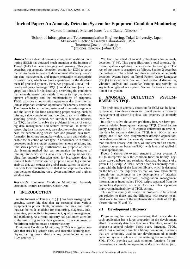
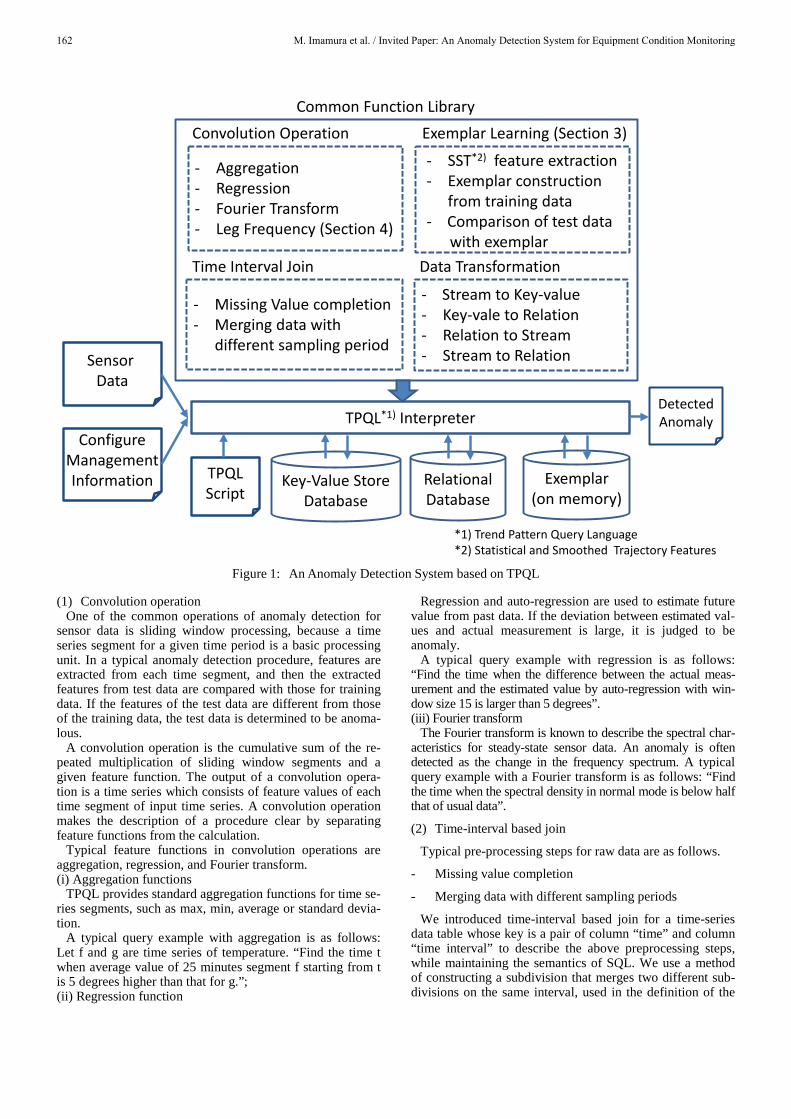
Figure 1 shows the overall structure of our system. A TPQL interpreter calls the common function library, key-value store database, and relational database, by means of a given TPQL script. A TPQL script describes anomaly condi-tions with the help of the function library, which is designed on the basis of the requirements that we have encountered through our experience in the development of practical ECM systems. Furthermore, configuration management information as input makes TPQL scripts separated from the parameters dependent on actual facilities. This separation improves maintainability of TPQL scripts.

This section mainly illustrates the problems to be solved, our solution to those, and the difference with respect to re-lated work. In terms of the implementation details of TPQL, please refer to [3] and [4].

2.1 Development Efficiency

Programming for data preprocessing that is specific to each application has a large proportion in the development effort for anomaly detection functions. Therefore, we aim to propose a general relation based query language, TPQL, which has a common function library containing functions that are commonly used in our development of anomaly detection systems, while also maintaining the semantics of SQL. TPQL provides two basic common functions for pre-processing: a convolution operation and a time-interval join.

International Journal of Informatics Society, VOL.8, NO.3 (2016) 161-169 161

ISSN1883-4566 ©2016 - Informatics Society and the authors. All rights reserved.

(1) Convolution operationOne of the common operations of anomaly detection for

sensor data is sliding window processing, because a time series segment for a given time period is a basic processing unit. In a typical anomaly detection procedure, features are extracted from each time segment, and then the extracted features from test data are compared with those for training data. If the features of the test data are different from those of the training data, the test data is determined to be anoma-lous.

A convolution operation is the cumulative sum of the re-peated multiplication of sliding window segments and a given feature function. The output of a convolution opera-tion is a time series which consists of feature values of each time segment of input time series. A convolution operation makes the description of a procedure clear by separating feature functions from the calculation.

Typical feature functions in convolution operations are aggregation, regression, and Fourier transform. (i) Aggregation functions

TPQL provides standard aggregation functions for time se-ries segments, such as max, min, average or standard devia-tion.

A typical query example with aggregation is as follows: Let f and g are time series of temperature. “Find the time t when average value of 25 minutes segment f starting from t is 5 degrees higher than that for g.”; (ii) Regression function

Regression and auto-regression are used to estimate future value from past data. If the deviation between estimated val-ues and actual measurement is large, it is judged to be anomaly.

A typical query example with regression is as follows: “Find the time when the difference between the actual meas-urement and the estimated value by auto-regression with win-dow size 15 is larger than 5 degrees”. (iii) Fourier transform

The Fourier transform is known to describe the spectral char-acteristics for steady-state sensor data. An anomaly is often detected as the change in the frequency spectrum. A typical query example with a Fourier transform is as follows: “Find the time when the spectral density in normal mode is below half that of usual data”.

(2) Time-interval based join

Typical pre-processing steps for raw data are as follows.

- Missing value completion

- Merging data with different sampling periods

We introduced time-interval based join for a time-seriesdata table whose key is a pair of column “time” and column “time interval” to describe the above preprocessing steps, while maintaining the semantics of SQL. We use a method of constructing a subdivision that merges two different sub-divisions on the same interval, used in the definition of the

Figure 1: An Anomaly Detection System based on TPQL

Key-Value Store Database

*1) Trend Pattern Query Language*2) Statistical and Smoothed Trajectory Features

TPQL*1) Interpreter

TPQLScript

ConfigureManagementInformation

Exemplar Learning (Section 3)

- SST*2) feature extraction- Exemplar construction

from training data- Comparison of test data

with exemplar

Convolution Operation

- Aggregation- Regression- Fourier Transform- Leg Frequency (Section 4)

Time Interval Join

- Missing Value completion- Merging data with

different sampling period

Data Transformation

- Stream to Key-value- Key-vale to Relation- Relation to Stream- Stream to Relation

RelationalDatabase

Exemplar (on memory)

Common Function Library

Sensor Data

DetectedAnomaly

M. Imamura et al. / Invited Paper: An Anomaly Detection System for Equipment Condition Monitoring162

Stieltjes integral, for joining tables with different time inter-vals.

A standard temporal query language TSQL [7] also sup-ports operation over time intervals, such as intersection and inclusion and so on, but does not support time-interval join.

2.2 Sensor Big Data Management There are a lot of sensors in a facility, so that a large

amount of data will be accumulated as time passes. If there are 10,000 sensors, sampling period is one second and one byte per one point, the amount of data is about 1 Gbytes per one day. If the number of sensors per device is 50, the total number of 10000 sensors would be reched by as little as 200 devices in a facility, or 200 products in the consumer market. Therefore, 10,000 sensors is not an excessive assumption. Furthermore, missing values often occur in sensor data, so relational databases that are frequently used in enterprise domains, may not be suitable, because they have excessively strict data management functions. We propose two functions. One is for data transformation and the other is for fast pro-cessing. (1) Data Transformation

With respect to storage, our system uses key-value storedatabase, which is often used for big data, and provides mu-tual transformation functions among key-value data, rela-tional data and stream data for developers to select a suitable data type in accordance with the purpose of processing in TPQL scripts. Generally speaking, key-value data are suita-ble for accumulating data, relational data are suitable for aggregation over relations, and stream data are suitable for data passing to external functions and time series analysis.

The typical stream query language CQL [8] is also a rela-tion-based one, and has a sliding window process as one of its basic operations. CQL provides the transformation be-tween relational data and stream data, that is, “Relation to Stream” and “Stream to Relation”. TPQL adds “Stream to Key-value” and “Key-value to Relation” as basic data trans-formation functions. (2) Exemplar Learning

With respect to fast processing, we proposed a compres-sion method that opearates by combining similar data seg-ments into one segment, in order to speed up anomaly detec-tion procedures. We call this method exemplar learning in this paper. Exemplar learning will be illustrated in the next section.

2.3 Feature Extraction Characteristics of Sensor Data

A lot of algorithms have been proposed for anomaly detec-tion [9]. We have a policy to select existing algorithms in accordance with our application requirements. Pre-processing for sensor data is as important as the anomaly detection algorithms themselves. The techniques for prepro-cessing are sometimes called feature engineering [10], and are a very important factor in determining the success of anomaly detection systems.

Vibrational behavior is very important for anomaly detec-tion. The Fourier transform is a useful and frequently used feature for steady state data, but it is not so useful for transi-ent or non-periodical data from our experience. We intro-duce a novel feature which we call leg frequency in order to calculate the frequency of variations in time series that in-

clude an upward trend and a downward trend alternatively. Leg frequency is treated as a feature function in convolution operation in TPQL.

Rain flow method [11],[12] in material mechanics is a re-lated work. It calculates the amplitude of deformation which causes the fatigues or the cracks form in materials. It calcu-lates the maximal pair of upward trend and downward trend at each maximal point. But our leg vibration analysis calcu-lates the frequency in a time series segment for given ampli-tude so that it can describe the degree of fluctuation for the given amplitude that is decided to distinguish anomaly from noise with domain knowledge.

A typical query with leg vibration analysis is used in de-tecting hunting in control systems. A query example is as follows: “Find the time when the number of the alternate oc-currences of upward and downward trends whose amplitude are above 3 ℃ during 30 minutes window is larger than 2”. In this example, 3 ℃ and 30 minutes are the parameter that are decid-ed by the application requirement.

Leg vibration analysis will be illustrated in section 4.

3 EXEMPLAR LERNING

3.1 Statistical and Smoothed Trajectory (SST) Features

We proposed statistical and smoothed trajectory (SST) features [5] that can capture the shape and the stochastic behavior of the time series within the window so that it can handle various types of sensor data.

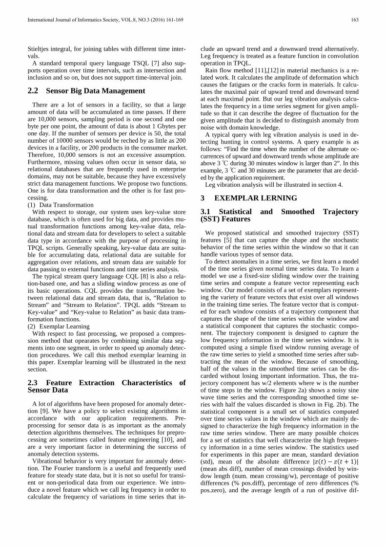
To detect anomalies in a time series, we first learn a model of the time series given normal time series data. To learn a model we use a fixed-size sliding window over the training time series and compute a feature vector representing each window. Our model consists of a set of exemplars represent-ing the variety of feature vectors that exist over all windows in the training time series. The feature vector that is comput-ed for each window consists of a trajectory component that captures the shape of the time series within the window and a statistical component that captures the stochastic compo-nent. The trajectory component is designed to capture the low frequency information in the time series window. It is computed using a simple fixed window running average of the raw time series to yield a smoothed time series after sub-tracting the mean of the window. Because of smoothing, half of the values in the smoothed time series can be dis-carded without losing important information. Thus, the tra-jectory component has w/2 elements where w is the number of time steps in the window. Figure 2a) shows a noisy sine wave time series and the corresponding smoothed time se-ries with half the values discarded is shown in Fig. 2b). The statistical component is a small set of statistics computed over time series values in the window which are mainly de-signed to characterize the high frequency information in the raw time series window. There are many possible choices for a set of statistics that well characterize the high frequen-cy information in a time series window. The statistics used for experiments in this paper are mean, standard deviation (std), mean of the absolute difference |𝑧𝑧(𝑡𝑡) − 𝑧𝑧(𝑡𝑡 + 1)| (mean abs diff), number of mean crossings divided by win-dow length (num. mean crossing/w), percentage of positive differences (% pos.diff), percentage of zero differences (% pos.zero), and the average length of a run of positive dif-


ferences divided by window length (avg. run of pos. diff/w). Here, 𝑧𝑧(𝑡𝑡) is the value of the raw time series at time 𝑡𝑡. Fig-ure 5(c) shows the vector of statistics for an example win-dow. This choice of statistics has worked well in practice across a variety of different time series, but as mentioned before other statistics would likely also work well. The tra-jectory component is half the length of the window (w/2 time steps), and the statistical component is 7 real numbers for a total of w/2+7 real values. We call this novel represen-tation Statistical and Smoothed Trajectory (SST) features.

3.2 Anomaly Detection using Exemplar Learning

One possible model for a time series is simply the set of all SST features that are computed from all overlapping win-dows of the time series. This model would be an inefficient representation because the overlapping windows would pro-duce many very similar feature vectors. A much more effi-cient model is created by finding a small set of exemplars that compactly represent the set of all SST features from the time series. An exemplar in this context is a representation of the SST features of a group of similar windows (overlap-ping or not) from the training time series. We use an ag-glomerative clustering algorithm to select SST exemplars from the set of all SST features for a time series.

The agglomerative clustering algorithm works as follows. After computing SST features for every window of the train-ing time series, a set of exemplars is learned by initially as-signing each SST feature as its own exemplar and then itera-tively combining the two nearest exemplars until the mini-mum distance between nearest exemplars is above a thresh-old. This is illustrated in Fig. 3.

We use Euclidean distance to measure the distance be-tween two exemplars:

𝑑𝑑𝑑𝑑𝑑𝑑𝑡𝑡�𝑓𝑓1,𝑓𝑓2� = ∑ �𝑓𝑓1. 𝑡𝑡(𝑑𝑑) − 𝑓𝑓2. 𝑡𝑡(𝑑𝑑)�2 +𝑤𝑤2𝑖𝑖=1

𝑤𝑤14∑ �𝑓𝑓1. 𝑑𝑑(𝑑𝑑) − 𝑓𝑓2. 𝑑𝑑(𝑑𝑑)�27𝑖𝑖=1

where 𝑓𝑓1 and 𝑓𝑓2 are two feature vectors, 𝑓𝑓𝑗𝑗 . 𝑡𝑡 is the length w/2 trajectory component of 𝑓𝑓𝑗𝑗, and 𝑓𝑓𝑗𝑗 . 𝑑𝑑 is the length 7 sta-tistical component of 𝑓𝑓𝑗𝑗 . The w/14 coefficient causes the statistical and trajectory components to be weighted equally.

Two exemplars are combined by a weighted average of the corresponding elements. The weight is the count of the number of feature vectors that have already been averaged into each exemplar divided by the total count. Each resulting exemplar is thus simply the overall average of the feature vectors that went into it. The threshold that determines when to stop combining exemplars is set to 𝜇𝜇 + 3𝜎𝜎 where 𝜇𝜇 is the mean of the Euclidean distances (𝑑𝑑𝑑𝑑𝑑𝑑𝑡𝑡�𝑓𝑓1,𝑓𝑓2�) between each initial SST feature vector and its nearest neighbor among the initial SST feature vectors and 𝜎𝜎 is the sample standard de-viation of these distances. The running time of this exemplar selection algorithm is 𝑂𝑂(𝑛𝑛2𝑤𝑤) (where 𝑛𝑛 is the length of the training time series and 𝑤𝑤 is the chosen window size).

After exemplar selection, each exemplar is associated with a set of original SST features that were averaged together to form the exemplar. The standard deviation of each element of the w/2+7 length feature vector is then computed and stored with each exemplar. These standard deviations are computed over the set of SST feature vectors associated with a particular exemplar. An exemplar is thus represented by w/2 + 7 mean elements and w/2 + 7 standard deviation elements. In our experiments, the final exemplar set is typi-cally between 1% and 5% of the total number of features (windows).

After the model is learned, anomalies are found in a test-ing time series as follows. For each window of the testing time series, an anomaly score is computed. This is done by first computing the SST feature of the window. Then the nearest neighbor exemplar to the SST feature is found. The distance function used is

Figure 2: Example time series window (a) along with its trajectory (b) and statistical components

(c) Statistical components

a) Raw time series subsequence

b) Trajectory Component (Smoothed time series)

c) Statistical component : mean: 0.25 std: 0.74 mean abs diff: 0.29 num mean crossings/w: 0.12 % pos.diff: 0.49 % zero.diff: 0.00 avg. run of pos. diff/w: 0.005


𝑑𝑑(𝑓𝑓, 𝑒𝑒) = �max �0,|𝑓𝑓. 𝑡𝑡(𝑑𝑑) − 𝑒𝑒. 𝑡𝑡(𝑑𝑑)|

𝑒𝑒.𝜎𝜎(𝑑𝑑)− 3�

𝑤𝑤2

𝑖𝑖=1

+𝑤𝑤 14

�max�0,|𝑓𝑓. 𝑑𝑑(𝑑𝑑) − 𝑒𝑒. 𝑑𝑑(𝑑𝑑)|

𝑒𝑒. 𝜀𝜀(𝑑𝑑)− 3�

7

𝑖𝑖=1

where 𝑓𝑓 is the SST feature vector for the current window consisting of a trajectory vector, 𝑓𝑓. 𝑡𝑡 and a statistical vector 𝑓𝑓. 𝑑𝑑, 𝑒𝑒 is an exemplar for the current dimension consisting of trajectory (𝑒𝑒. 𝑡𝑡) and statistical (𝑒𝑒. 𝑑𝑑) vectors as well as the corresponding standard deviation vectors, 𝑒𝑒.𝜎𝜎 for the trajec-tory component and 𝑒𝑒. 𝜀𝜀 for the statistical component.

This distance corresponds to assigning 0 distance for each element of the trajectory or statistical component that is less than 3 standard deviations from the mean and otherwise assigning the absolute value of the difference divided by the standard deviation for each element that is more than 3 standard deviations from the mean. In equation 2 and in our experiments, the statistical component is given equal weighting to the trajectory component, although this weighting can be changed based on the application.

4 LEG VIBRATION ANALYSIS

Facility maintenance in buildings, plants, or factories needs to calculate the frequency of variations in sensor data in order to detect a sign of failure or deterioration. Fink et al. proposed a leg search method [13] to find a global trend in a time-series including small variations such as noise. The dotted lines in Fig. 4 are examples of legs. Both lines show the global upward trend that includes local up-down seg-ments.

However, their method treats only single legs so that it can find an upward or downward trend, but can't catch the fre-quency of variations. We developed leg vibration analysis that can calculate the frequency of variations in time-series that includes upward trends and downward trends that can appear alternately and iteratively. We showed an algorithm whose calculation order is linear in the window size. In con-trast, the computational order of a naïve algorithm is factori-al in the square of window size.

Definition: time series X, sbsequences X[p:q] A Time Series X=[x1,…,xm] is a continuous sequence of

real values. The value of the i-th time point is denoted by X[i] = xi.

Figure 3: Illustration of agglomerative clustering for learning exemplars. The exemplars (which are SST feature vectors) are represented by blue rectangles. At each iteration the exemplars with minimum distance between them are averaged together using a weighted average. This process is repeated until the minimum

distance is above a threshold.


A Time Series subsequence s = [xp, xp+1,...,xq] = X[p:q] is a continuous subsequence of X starting at position p and ending at position q. We denote the starting time point, the ending time point, and the length of a subsequence l by start, end and length respectively:

start(s) ≡ p end(s) ≡ q

length(s) ≡ q-p+1

Definition: Leg Let X be time series. An upward leg l = X[p:q] is a subsequence of X that satis-

fies the following conditions from (1) to (3). ∀𝑑𝑑. 𝑝𝑝 ≤ 𝑑𝑑 ≤ 𝑞𝑞 𝑋𝑋[𝑝𝑝] < 𝑋𝑋[𝑑𝑑] < 𝑋𝑋[𝑞𝑞] (1)

𝑋𝑋[𝑝𝑝 − 1] ≥ 𝑋𝑋[𝑝𝑝] (2) 𝑋𝑋[𝑞𝑞] ≥ X[𝑞𝑞 + 1] (3) A downward leg l = X[p:q] is a subsequence of X that sat-

isfies the following conditions from (4) to (6) ∀𝑑𝑑. 𝑝𝑝 ≤ 𝑑𝑑 ≤ 𝑞𝑞 𝑋𝑋[𝑝𝑝] > 𝑋𝑋[𝑑𝑑] > 𝑋𝑋[𝑞𝑞] (4) 𝑋𝑋[𝑝𝑝 − 1] ≤ 𝑋𝑋[𝑝𝑝] (5) 𝑋𝑋[𝑞𝑞] ≤ X[𝑞𝑞 + 1] (6)

If l is an upward leg or downward leg, l is called a leg.

Definition: Sign and amplitude of a leg Let X[p:q] be a leg l . We define the sign and amplitude of

a leg l by the following. We denote them by amp and sign respectively:

sign(𝑙𝑙) ≡ sign(𝑋𝑋[𝑞𝑞] − 𝑋𝑋[𝑝𝑝]) amp(𝑙𝑙) ≡ abs(𝑋𝑋[𝑞𝑞] − 𝑋𝑋[𝑝𝑝])

Definition: Leg Vibration Sequence Let l1, l2,.., ln be legs, and A be a positive real number. A

leg vibration sequence with amplitude A is a leg sequence u = [l1, l2,.., ln] that satisfies the following conditions from (7) to (9).

For 1≦i≦n-1 end(li) ≦start(li+1) (7) For 1≦i≦n amp(li) ≧ A (8) For 1≦i≦n-1 sign (li) × sign (li+1) < 0 (9)

Definition: Frequency of a leg vibration sequence Let v = [l1, l2,.., ln] be a leg vibration sequence. The start,

end, length, sign, amplitude and frequency for a leg vibra-tion sequence v are defined as follows. We denote them by start, end, length, amp and freq respectively:

start(v) ≡ start(𝑙𝑙1) end(v) ≡ end(𝑙𝑙𝑛𝑛) length(v) ≡ n

sign(v) ≡ sign(𝑙𝑙1) amp(v) ≡ min

𝑖𝑖amp( 𝑙𝑙𝑖𝑖)for 1 ≦ 𝑑𝑑 ≦ 𝑛𝑛

freq(v) ≡ sign(𝑣𝑣) × length(𝑣𝑣)

Definition: Leg vibration sequence set of a subsequence for amplitude A

Let X[p:q] and A be a subsequence of time series X and amplitude respectively. Leg vibration sequence set for am-plitude A 𝑉𝑉(𝑋𝑋[𝑝𝑝: 𝑞𝑞],𝐴𝐴) is defined by a set of leg vibration sequences v = [l1, l2,.., ln] that satisfy the following condi-tions from (10) to (12).

amp(v) ≧ A (10) p ≦start(v) (11) end(v) ≦ q (12)

Definition: Leg frequency of a subsequence for amplitude A Let 𝑉𝑉(𝑋𝑋[𝑝𝑝: 𝑞𝑞],𝐴𝐴) be a leg vibration sequence set of a sub-

sequence 𝑋𝑋[𝑝𝑝: 𝑞𝑞] for an amplitude A. Leg frequency 𝑓𝑓𝑓𝑓𝑒𝑒𝑞𝑞𝐴𝐴 of a subsequence X[p:q] for A is defined by below.

freq𝐴𝐴(𝑋𝑋[𝑝𝑝: 𝑞𝑞]) ≡ sign(𝑣𝑣max) × length(𝑣𝑣max) where 𝑣𝑣max = argmax

𝑣𝑣∈𝑉𝑉(𝑋𝑋[𝑝𝑝:𝑞𝑞],𝐴𝐴)length(v) (13)

Leg frequency is well defined because 𝑣𝑣max is not unique but the sign of 𝑣𝑣maxs is unique due to the lemma below.

Lemma: Let 𝑉𝑉(𝑋𝑋[𝑝𝑝: 𝑞𝑞],𝐴𝐴) be a leg vibration sequence set of a subsequence 𝑋𝑋[𝑝𝑝: 𝑞𝑞] for amplitude A. The signs of leg vibration sequences that satisfy (13) are the same.

Proof. We assume that u = [l1, l2,.., ln] and v = [m1, m2,.., mn] are leg vibration sequences where both u and v have the maximal length n in 𝑉𝑉(𝑋𝑋[𝑝𝑝: 𝑞𝑞],𝐴𝐴) and have different signs. We will show this assumption implies contradiction. With-out loss of generality, we can assume that sign(u) is positive and sign(v) is negative; leg l1 is upward leg and m1 is down-ward leg.

Since l1 and m1 cross, either one is included by the other, or either one proceeds the other, one of the following condi-tions is true.

start(l1) < start(m1) < end(l1) < end(m1) (14) start(m1) < start(l1) < end(m1) < end(l1) (15) start(l1) < start(m1) < end(m1) < end(l1) (16) start(m1) < start(l1) < end(l1) < end(m1) (17) start(l1) < end(l1) ≤ start(m1) < end(m1) (18) start(m1) < end(m1) ≤ start(l1) < end(l1) (19)

The definition of leg implies that the above magnitude re-lations in the formulas from (14) to (17) satisfy not equality but inequality.

First, we will deduce the contradiction when the condition (14) is true. Since l1 is an upward leg, X[start(m1)] <X[end(l1)]. Since m1 is an downward leg, X[start(m1)] >X[end(l1)]. These equations contradict each other. When thecondition (15) is true, a proof is in the same way.

Secondary, we will deduce the contradiction when the condition (16) is true. Since amp(m1) ≧ A and l1 an upward leg, l1_1 = X[start(l1): start(m1)] is an upward leg whose am-plitude is greater than or equal to A. Therefore, [l1_1, m1, m2,.., mn] is a leg sequence whose length is n + 1. It contra-dicts that v has the maximal length n in 𝑉𝑉(𝑋𝑋[𝑝𝑝: 𝑞𝑞],𝐴𝐴). When the condition (17) is true, a proof is in the same way.

Lastly, we will deduce the contradiction when the condi-tion (18) is true. Since [l1, m1, m2,.., mn] is a leg sequence whose length is n + 1. It contradicts that v has the maximal

Figure4: Leg


length n in 𝑉𝑉(𝑋𝑋[𝑝𝑝: 𝑞𝑞],𝐴𝐴). When the condition (19) is true, a proof is in the same way.

Therefore, the initial assumption – u and v have different sign – must be false. □

Definition: Leg Frequency 𝑓𝑓𝑓𝑓𝑒𝑒𝑞𝑞𝑋𝑋,𝐴𝐴,𝑊𝑊(𝑡𝑡) Let X, A, W are time series, amplitude and window size re-

spectively. A Leg Frequency of X at time t with A and W, 𝑓𝑓𝑓𝑓𝑒𝑒𝑞𝑞𝑋𝑋,𝐴𝐴,𝑊𝑊(𝑡𝑡), is defined as follows:

𝑓𝑓𝑓𝑓𝑒𝑒𝑞𝑞𝑋𝑋,𝐴𝐴,𝑊𝑊(𝑡𝑡) ≡ 𝑓𝑓𝑓𝑓𝑒𝑒𝑞𝑞𝐴𝐴(𝑋𝑋[𝑡𝑡: 𝑡𝑡 + 𝑊𝑊 − 1])

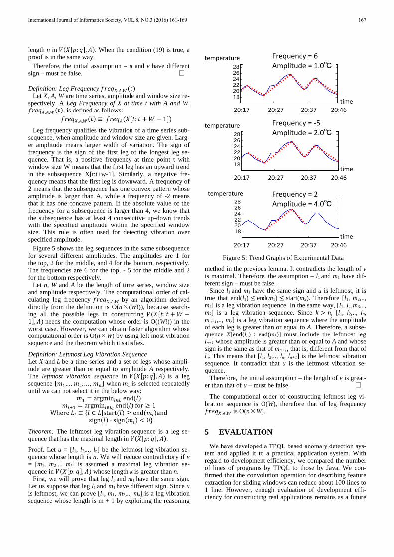
Leg frequency qualifies the vibration of a time series sub-sequence, when amplitude and window size are given. Larg-er amplitude means larger width of variation. The sign of frequency is the sign of the first leg of the longest leg se-quence. That is, a positive frequency at time point t with window size W means that the first leg has an upward trend in the subsequence X[t:t+w-1]. Similarly, a negative fre-quency means that the first leg is downward. A frequency of 2 means that the subsequence has one convex pattern whose amplitude is larger than A, while a frequency of -2 means that it has one concave pattern. If the absolute value of the frequency for a subsequence is larger than 4, we know that the subsequence has at least 4 consecutive up-down trends with the specified amplitude within the specified window size. This rule is often used for detecting vibration over specified amplitude.

Figure 5 shows the leg sequences in the same subsequence for several different amplitudes. The amplitudes are 1 for the top, 2 for the middle, and 4 for the bottom, respectively. The frequencies are 6 for the top, - 5 for the middle and 2 for the bottom respectively.

Let n, W and A be the length of time series, window size and amplitude respectively. The computational order of cal-culating leg frequency 𝑓𝑓𝑓𝑓𝑒𝑒𝑞𝑞𝑋𝑋,𝐴𝐴,𝑊𝑊 by an algorithm derived directly from the definition is O(n×(W!)), because search-ing all the possible legs in constructing 𝑉𝑉(𝑋𝑋[𝑡𝑡: 𝑡𝑡 + 𝑊𝑊 −1],𝐴𝐴) needs the computation whose order is O((W!)) in the worst case. However, we can obtain faster algorithm whose computational order is O(n×W) by using left most vibration sequence and the theorem which it satisfies.

Definition: Leftmost Leg Vibration Sequence Let X and 𝐿𝐿 be a time series and a set of legs whose ampli-tude are greater than or equal to amplitude A respectively. The leftmost vibration sequence in 𝑉𝑉(𝑋𝑋[𝑝𝑝: 𝑞𝑞],𝐴𝐴) is a leg sequence [𝑚𝑚1,.., 𝑚𝑚𝑖𝑖,…, 𝑚𝑚𝑛𝑛] when 𝑚𝑚𝑖𝑖 is selected repeatedly until we can not select it in the below way:

𝑚𝑚1 = argmin𝑙𝑙∈𝐿𝐿 end(𝑙𝑙) 𝑚𝑚𝑖𝑖+1 = argmin𝑙𝑙∈𝐿𝐿𝑖𝑖 end(𝑙𝑙) for ≥ 1

Where 𝐿𝐿𝑖𝑖 ≡ {𝑙𝑙 ∈ 𝐿𝐿|start(𝑙𝑙) ≥ end(𝑚𝑚𝑖𝑖)and sign(𝑙𝑙) ⋅ sign(𝑚𝑚𝑖𝑖) < 0}

Theorem: The leftmost leg vibration sequence is a leg se-quence that has the maximal length in 𝑉𝑉(𝑋𝑋[𝑝𝑝: 𝑞𝑞],𝐴𝐴).

Proof. Let u = [l1, l2,.., ln] be the leftmost leg vibration se-quence whose length is n. We will reduce contradictory if v = [m1, m2,.., mk] is assumed a maximal leg vibration se-quence in 𝑉𝑉(𝑋𝑋[𝑝𝑝: 𝑞𝑞],𝐴𝐴) whose length k is greater than n.

First, we will prove that leg l1 and m1 have the same sign. Let us suppose that leg l1 and m1 have different sign. Since u is leftmost, we can prove [l1, m1, m2,.., mk] is a leg vibration sequence whose length is m + 1 by exploiting the reasoning

method in the previous lemma. It contradicts the length of v is maximal. Therefore, the assumption – l1 and m1 have dif-ferent sign – must be false.

Since l1 and m1 have the same sign and u is leftmost, it is true that end(l1) ≤ end(m1) ≤ start(m2). Therefore [l1, m2,.., mk] is a leg vibration sequence. In the same way, [l1, l2, m3,.., mk] is a leg vibration sequence. Since k > n, [l1, l2,.., ln, mn+1,.., mk] is a leg vibration sequence where the amplitude of each leg is greater than or equal to A. Therefore, a subse-quence X[end(ln) : end(mk)] must include the leftmost leg ln+1 whose amplitude is greater than or equal to A and whose sign is the same as that of mn+1, that is, different from that of ln. This means that [l1, l2,.., ln, ln+1] is the leftmost vibration sequence. It contradict that u is the leftmost vibration se-quence.

Therefore, the initial assumption – the length of v is great-er than that of u – must be false. □

The computational order of constructing leftmost leg vi-bration sequence is O(W), therefore that of leg frequency 𝑓𝑓𝑓𝑓𝑒𝑒𝑞𝑞𝑋𝑋,𝐴𝐴,𝑊𝑊 is O(n×W).

5 EVALUATION

We have developed a TPQL based anomaly detection sys-tem and applied it to a practical application system. With regard to development efficiency, we compared the number of lines of programs by TPQL to those by Java. We con-firmed that the convolution operation for describing feature extraction for sliding windows can reduce about 100 lines to 1 line. However, enough evaluation of development effi-ciency for constructing real applications remains as a future

20:17 20:27 20:37 20:46

20:17 20:27 20:37 20:46

20:17 20:27 20:37 20:46

Frequency = 6 Amplitude = 1.0℃

temperature

time

temperature

time

time

Frequency = -5Amplitude = 2.0℃

Frequency = 2Amplitude = 4.0℃

temperature

Figure 5: Trend Graphs of Experimental Data


work. The rest of this section shows the result of processing time. (1) TPQL

We confirmed that our system satisfies the processing timethat are required by our real application. Our requirement of ECM for buildings is that the processing must be completed within one day for the following conditions: - 3 anomaly detection scenarios for each signal- 5,000 signals with sampling period one minute in half a

yearThe detail results and the conditions in the experiment are

described in [4]. (2) Exemplar Learning

We compared our algorithm to the simple yet effectiveBrute Force Euclidian Distance (BFED) algorithm [14] which has proven to be the most accurate over a variety of different testing time series [15]. Data for the experiment are 24 data sets that are available from the paper [16] and 2 syn-thesized data sets. The result shows that our algorithm is about from 5 times to 100 times faster than the BFED algo-rithm without losing accuracy. The detail results and the conditions in the experiment are described in [5]. (3) Leg vibration analysis

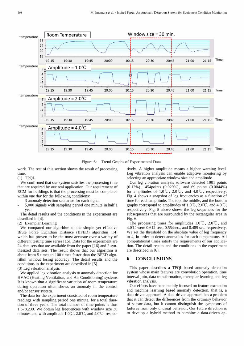
We applied leg vibration analysis to anomaly detection forHVAC (Heating Ventilation, and Air Conditioning) systems. It is known that a significant variation of room temperature during operation often shows an anomaly in the control and/or sensor system.

The data for the experiment consisted of room temperature readings with sampling period one minute, for a total dura-tion of three years. The total number of time points is thus 1,578,239. We obtain leg frequencies with window size 30 minutes and with amplitude 1.0℃, 2.0℃, and 4.0℃, respec-

tively. A higher amplitude means a higher warning level. Leg vibration analysis can enable adaptive monitoring by selecting an appropriate window size and amplitude.

Our leg vibration analysis software detected 1901 points (0.12%)，454points (0.029%)，and 69 points (0.0044%) for amplitudes of 1.0℃ , 2.0℃ , and 4.0℃ , respectively. Fig. 4 shows a snapshot of leg frequencies as a function of time for each amplitude. The top, the middle, and the bottom graphs correspond to amplitudes of 1.0℃, 2.0℃, and 4.0℃, respectively. Fig. 5 above shows the leg sequences for the subsequences that are surrounded by the rectangular area in Fig. 6.

The processing times for amplitudes 1.0℃ , 2.0℃ , and 4.0℃ were 0.612 sec., 0.554sec., and 0.489 sec. respectively. We set the threshold on the absolute value of leg frequency to 4, in order to detect anomalies for each temperature. All computational times satisfy the requirements of our applica-tion. The detail results and the conditions in the experiment are described in [6].

6 CONCLUSIONS

This paper describes a TPQL-based anomaly detection system whose main features are convolution operation, time interval join, data transformation, exemplar learning and leg vibration analysis.

Our efforts have been mainly focused on feature extraction and machine learning based anomaly detection, that is, a data-driven approach. A data-driven approach has a problem that it can detect the differences from the ordinary behavior of sensor data, but it cannot distinguish the symptoms of failures from only unusual behavior. Our future direction is to develop a hybrid method to combine a data-driven ap-

Figure 6: Trend Graphs of Experimental Data

temperature

temperature

temperature

temperature

時区間A 時区間B 時区間C 時区間D

Amplitude = 1.0℃

Room Temperature28242016

840

-4-8

19:15 19:30 19:45 20:00 10:15 20:30 20:45 21:00 21:15

19:15 19:30 19:45 20:00 10:15 20:30 20:45 21:00 21:15

62

-2-6

19:15 19:30 19:45 20:00 10:15 20:30 20:45 21:00 21:15

420

-2-4

19:15 19:30 19:45 20:00 10:15 20:30 20:45 21:00 21:15

Amplitude = 2.0℃

Amplitude = 4.0℃

Window size = 30 min.

Time

Time

Time

Time


proach with a physical model-based approach with equip-ment domain knowledge in order to explain whether anoma-lous behavior is actually a symptom of a failure.

REFERENCES

[1] J. Zheng, D. Simplot-Ryl, C. Bisdikian, H.T.Mouftah: “TheInternet of Things [Guest Editorial],” Communications Maga-zine, IEEE , Vol.49, No.11, pp.30-31 (2011).

[2] M. Imamura, D. Nikovski, Z. Sahinoglu, M. Jones: “A Surveyon Machine Learning for Equipment Condition Monitoring Us-ing Sensor Big Data,” IIEEJ Transactions on Image Electronicsand Visual Computing Vol.2 No.2, pp. 112-121 (2014).

[3] M. Imamura, S. Takayama, and T. Munaka: “A stream querylanguage TPQL for anomaly detection in facility management,”The 16th International Database Engineering & ApplicationsSymposium (IDEAS '12), pp. 235-238 (2012).

[4] M. Imamura,T. Takeuchi, S. Kitagami, M. Kanno, T. Munaka:“Time Series Data Query Language TPQL for anomaly detec-tion in facility,” Journal C of Electronics and Communicationsin Japan,Vol.134, No.1, pp. 156-167 (2014). (in Japanese).

[5] M. Jones and D. Nikovski and M. Imamura and T. Hirata: “Ex-emplar Learning for Extremely Efficient Anomaly Detection inReal Valued Time Series,” Data Mining and Knowledge Dis-covery (DAMI), First online: 25, pp 1-28 (2016).

[6] M. Imamura, T. Nakamura, H. Shibata, N. Hirai, S. Kitagami, T.Munaka: “Leg Vibration Analysis for Time Series,” IPSJ Jour-nal, Vol. 57, No.4, pp.1303-1318 (2016). (in Japanese).

[7] R. T. Snodgrass (Ed.): The TSQL2 Temporal Query Language.Kluwer (1995).

[8] A. Arasu, S. Babu, J. Widom: “The CQL continuous querylanguage: semantic foundations and query execution,” The In-ternational Journal on Very Large Data Bases archive, Vol. 15,No. 2, (2006).

[9] V. Chandola, A. Banerjee, V. Kumar: “Anomaly detection: asurvey,” ACM Comput Survey, Vol. 41, No. 3 (2009).

[10] W. Yan: “Feature Engineering for PHM applications,” The 7thAnnual Conference of the Prognostics and Health ManagementSociety,http://www.phmsociety.org/sites/phmsociety.org/files/FeatureEngineeringTutorial_2015PHM_V2.pdf (2015).

[11] T. Endo, M. Matsuishi, K. Kounaga, K. Kobayashi, K.Takahashi: “Rain Flow Method and Its Application,” ResearchReport of Kyushu Institute of Technology, http://www-it.jwes.or.jp/qa/details.jsp?pg_no=0040020170 (1974).

[12] I. Rychlik: “A new definition of the rainflow cycle countingmethod,” International journal of fatigue Vol. 9. No. 2, pp.119-121 (1987).

[13] E. Fin, B. P. Kevin: “Indexing of Compressed Time series,”DATA MINING IN TIME SERIES DATABASES, World Sci-entific, pp. 43-65 (2004).

[14] T. RakthanmanonT, B. Campana B, A. Mueen, G. Batista, B.Westover, Q. Zhu, J. Zakaria, E. Keogh Searching and miningtrillions of time series subsequences under dynamic time warp-ing. 18th ACM SIGKDD international conference onknowledge discovery and data mining, pp 262–270 (2012).

[15] H. Ding, G. Trajcevski, P. Scheuermann, X. Wang, and E.Keogh: “Querying and Mining of Time Series Data: Experi-mental Comparison of Representations and Distance Measures,”VLDB 2008, pp.1542-1552 (2008).

[16] E. Keogh, J. Lin, A. Fu: “HOT SAX: finding the most unusu-al time series subsequence: algorithms and applications,” TheFifth IEEE international conference on data mining, pp. 226–233, www.cs.ucr.edu/eamonn/discords/ (2005).

(Received September,30,2015) (Revised June 10,2016)

Makoto Imamura He received a M.E. degree from Kyoto Uni-versity of Applied Mathematics and Physics in 1986 and a Ph.D. degree from Osaka University of the Information Science and Technology in 2008. He is a professor of the school of In-

formation and Telecommunication Engineering at Tokai University. He had been worked as a research staff at the Information Technology R&D Center in Mitsubishi Electric Corporation until 2015. He has worked on datamining methods for prognostics and health management and cyber-physical production system.

Daniel Nikovski He received a PhD in robotics from Carnegie Mellon University in 2002, and is presently a senior member of research staff and group manager of the Data Analytics group at Mitsubishi Electric Research La-boratories. He has worked on probabilistic methods for reason-

ing, learning, planning, and scheduling, and their applications to hard industrial problems. He is a member of IEEE.

Michael Jones He received a Ph.D. degree from the Electrical

Engineering and Computer Sci-ence department of the Massachu-setts Institute of Technology (MIT) in 1997, and is currently a senior principal member of the research staff at Mitsubishi Elec-tric Research Laboratories. He has

worked mainly on problems in computer vision, but recently has also focused on time series analysis.


Documents

Invited Paper: An Anomaly Detection System for Equipment ... · Invited Paper: An Anomaly Detection System for Equipment Condition Monitoring . Makoto Imamura *, Michael Jones **,