Investment in Electricity Markets with Asymmetric

Technologies

Talat S. Genc∗

University of Guelph

Henry Thille

University of Guelph

April 29, 2010

Abstract

Capacity investments in electricity markets is one of the main issues in the restruc-

turing process to ensure competition and enhance system security of networks. We

study competition between hydro and thermal electricity generators under demand

uncertainty. Producers compete in quantities and each is constrained: the thermal

generator by capacity and the hydro generator by water availability. We analyze a

two-period game emphasizing the incentives for capacity investments by the thermal

generator. We characterize both Markov perfect and open-loop equilibria. In the

Markov perfect equilibrium, investment is discontinuous in initial capacity and higher

than it is in the open-loop equilibrium. However, since there are two distortions in

the model, equilibrium investment can be either higher or lower than the e�cient

investment.

Keywords: Electricity markets; Dynamic game; Duopoly; Capacity investment.

JEL codes: D24, L13, L94

∗We are grateful for comments and suggestions from Stanley Reynolds, the corresponding editor, anony-mous referees and seminar participants at several conferences and workshops where this paper was presented.Both authors acknowledge research support from SSHRC, Canada. The �rst author is the correspondingauthor. Address: University of Guelph, Dept. of Economics, Guelph, ON, N1G2W1, Canada. Email:tgenc@uoguelph.ca. Phone: 1.519.824.4120 x56106. Fax: 1.519.763.8497

1 Introduction

It is common to �nd alternative electricity generation technologies coexisting in a market.

In many jurisdictions, electricity is generated from a mix of thermal (coal, oil, gas), nuclear,

and hydro generation plants. Growth of the demand for electricity has meant that increased

generation capacity is desired in many jurisdictions. Especially in deregulated markets, new

generation capacity is not easily constructed for the larger, low marginal cost, generation

technologies such as hydro and nuclear.

The main issue that we address in this paper is that of investment in new thermal

generation capacity in the presence of a large hydro competitor.1 Following deregulation

and in combination with demand growth, investment in new generation capacity occurred in

many jurisdictions and continents (most signi�cantly in Europe and South America). Given

regulatory and environmental hurdles and substantial �xed costs, new hydro development

is often not an option. In this case, new capacity is commonly provided by thermal plants.

Since the incentive to invest in new capacity depends on the expected distribution of future

prices, the extent to which incumbent hydro generation a�ects the distribution of prices

will have an e�ect on investment in thermal capacity.

Although there has been much recent interest in models of electricity markets, there has

not been much analysis of the implications for market performance when one of the pro-

ducers has signi�cant hydroelectric generation capability. Crampes and Moreaux [4] model

an electricity market in which a hydro producer uses a �xed stock of water over two periods

facing competition from a thermal producer. Bushnell [2] examines a Cournot oligopoly

with fringe producers in which each producer controls both hydro and thermal generation

facilities. Both hydro and thermal units face capacity constraints and the producers must

decide how to allocate the available water over a number of periods. Scott and Read [18]

develop a Cournot model of mixed hydro/thermal generation that is calibrated to the New

Zealand wholesale electricity market. They focus on the e�ect of forward contracting, con-

cluding that high levels of contracting are necessary to approach an e�cient outcome. These

papers all focus on the allocation of water by the hydro producers. In contrast, we focus

on the longer term issue of investment by the thermal producer and abstract away from

concerns about water use. 2

In restructured electricity markets, the importance of having excess market capacity

through capacity investments has been stressed (see Roques, Newbery, and Nuttall [17],

Murphy and Smeers [13], Cramton and Stoft [5], Joskow [14], among others) for the sake

of more competitive outcomes and, importantly, of system security so that possible supply

disruptions o�set and/or unexpected peak demand met. In the past, cost-of-service regula-

tion enabled investors to recoup their investment costs through regulated rates. However,

in deregulated markets investors are motivated by pro�ts and it is the purpose of this paper

1We describe the low cost generation technology as hydroelectric throughout this paper. The modelequally applies to any low marginal cost technology with a capacity constraint. As we are focusing onlonger-term investment dynamics, we do not model shorter-term water �ow dynamics explicitly.

2Papers which focus on competition between hydro generators include Ambec and Doucet [1], andGarcia, Reitzes and Stacchetti [6].

2

to examine these incentives.

There are some recent papers that have examined investment incentives in electricity

markets. Murphy and Smeers [13] examine generation capacity investments in open-loop

and closed-loop Cournot duopolies. Each duopolist makes investments in production ca-

pacities. In the open-loop game, capacities are simultaneously built and sold in long-term

contracts, in the closed-loop game, however, capacities invested in the �rst stage and then

they are sold in the second stage in a spot market. They �nd that market outcomes (in-

vestments and outputs) in the closed-loop game are in between the open-loop game and

the e�cient outcomes. Bushnell and Ishii [3] study a simulation model of a discrete-time

dynamic Cournot game in which �rms make lumpy investment decisions. They calculate

the Markov perfect equilibrium investment levels in oligopoly. They �nd that uncertainty

in demand growth can delay investment. Garcia and Shen [7] characterize Markov perfect

equilibrium capacity expansion plans for oligopoly. They �nd that Cournot �rms underin-

vests relative to the social optimum. Garcia and Stacchetti [8] study a dynamic Bertrand

game with capacity constraints with random demand growth and periodic investments.

They �nd that in some equilibria total capacity falls short of demand, and hence system

security is jeopardized. They also �nd that price caps do not a�ect the optimum invest-

ment levels. Most of these papers assume symmetric technologies with constant marginal

cost of production. In our paper, we assume asymmetric technologies with di�erent cost

structures. This is an important feature in electricity generation industry, which is the

focus of this paper. We also compare di�erent behavioral strategies (Markov perfect versus

open-loop) that might be used by power generators before making investment decisions.

We examine a two-period duopoly market with one �rm operating a hydroelectric gen-

erating plant and another operating a thermal generating plant. Both �rms have capacity

constraints, but only the thermal producer is able to invest in increasing its capacity. In

the �rst period both producers choose their outputs, and the thermal player also chooses

investment level that will be productive in the following period. In the second period both

players simultaneously choose their production levels given their capacities. Demand for

electricity in the second period is stochastic due to uncertain demand growth. We analyze

the choice of capacity by the thermal producer under demand uncertainty and characterize

both the Markov perfect and S-adapted open-loop equilibria under both binding and non-

binding hydro production constraints. We �nd that thermal investment is higher under

Markov perfect information and this investment may be either higher or lower than the ef-

�cient. We also �nd that optimal investment is a discontinuous function of initial capacity

under the Markov perfect equilibrium, and it is a continuous function under the open-loop

structure.

2 The Model

The �rms compete over two periods, t = 0, 1. In period 0, inverse demand is known to

be P0(Q) = D − Q, with D a constant and Q the total output of the two �rms. Inverse

3

demand in period 1 is random:

P1(Q) =

{D + δ −Q with probability u

D − δ −Q with probability d(1)

with u+ d = 1, and δ > δ ≥ 0. This demand model allows di�erent jump levels in demand

intercept, including increasing or �at demand levels in period 1. The expected demand in

period 1 is δ(2u−1), whenever δ = δ = δ. Hence, the demand growth will be positive as long

as u > 0.5. The demand model is a discrete time version of the Brownian motion process,

which is a commonly used stochastic demand for capital investment dynamic games. Several

reasons may cause demand growth in electricity such as population growth and/or GDP

growth which may necessitate more electricity usage for production.

We note that the point elasticity of demand changes if there is growth.3 It is not only

demand growth that a�ects the elasticity: as we show below the thermal investment results

in a change in future outputs which also imply di�erent elasticities. Indeed, some authors,

for example Pineau and Murto [15], and Genc and Sen [10], reason that price elasticity of

demand changes with respect to base load and peak demand.4

There are two types of technologies in the industry: a hydroelectric generator owns gen-

eration units that use water held behind dams to spin the electric generators and a thermal

electric generator owns thermal units that burn fossil fuel to turn the turbine. These dif-

ferent generation technologies result in di�erent cost functions for the two �rms. Thermal

generation is governed by the cost function C(q) = c1q + (c2/2)q2 for thermal output (q)

less than the thermal generator's capacity, which we denote by Kt at time t.5 The ther-

mal producer begins the game with K0 units of available generation capacity and has the

option of increasing the capacity through investment in period zero, I0. In period one, the

thermal producer then has capacity of K1 = K0 + I0, and investment is irreversible: I0 ≥ 0and capacity does not depreciate. Investment costs are modeled as a convex function of

investment: e1I20/2. This convex investment cost function may stem from adjustment costs,

which are due to costs of installing and/or removing equipment (see Reynolds [16]). This

assumed investment cost imposes the strong assumption of decreasing returns to scale in

capacity investment. Although clearly unrealistic for new plant construction, it is perhaps

more reasonable for the incremental capacity addition we are thinking about here. We

could add a �xed cost to investment to allow for some increasing returns to scale, however,

if this �xed cost were substantial it would change the analysis considerably as the hydro

producer might be able to deter thermal investment entirely. Although investment deter-

rence is interesting in its own right, we wish to focus on analyzing the level of investment

3This observation was pointed out by a referee.4To keep the elasticities across the demand variations constant, one could employ a constant elasticity

demand model. However, this would complicate the analysis as to obtain closed form solutions.5This cost function nests the linear portion of the costs but excludes �xed costs. The results of the

paper would not qualitatively change if we allow c2 to approach zero. Alternatively, this quadratic costfunction may represent the approximation of total costs for the portfolio of di�erent fossil fuels used in powergeneration process. Also, we do not model the transmission network, and hence assume away transmissionconstraints, transmission loss and congestion issues.

4

given that it occurs. Hence we suppress the �xed cost component of the thermal pro-

ducer's investment cost function, implicitly assuming that any �xed costs associated with

investment are su�ciently small as to not deter the thermal producer from investing. This

approach is consistent with, among others, Pineau and Murto [15], and Genc, Reynolds

and Sen [9] who use similar cost functions. Actions taken by the thermal producer consist

of investment and production in period 0 and production in each of the period 1 demand

states: (I0, q0, q1u, q1d).6

Hydroelectric power generation is generally thought of as having lower operating costs

which we model by assuming that the marginal cost of production for hydro units is zero.7

In each period there is a maximal amount of hydro electricity that can be generated denoted

by W0. We think of this capacity as the carrying capacity of the reservoir. Essentially, we

are assuming that there is su�cient in�ow of water between periods 0 and 1 to restore

W0 by the beginning of period 1.8 As such, one could think of our hydro producer as

any generator with a low marginal cost but �xed capacity (such as one with a nuclear

generation technology). The hydro producer must choose three actions in this game: period

0 production and period 1 production in each of the two demand states. We denote a vector

of hydro producer actions as (h0, h1u, h1d).It will be useful in the presentation of the results to let qcu and qcd denote the Cournot

equilibrium (interior solution) thermal outputs in the �rst period game when no constraints

bind and qc0 the corresponding quantity in period 0, i.e.,

qc0 ≡D − 2c13 + 2c2

, qcd ≡D − δ − 2c1

3 + 2c2, qcu ≡

D + δ − 2c13 + 2c2

. (2)

The timing of the game is as follows. In period 0, players choose production quantities

simultaneously and independently to maximize their own pro�ts. At the same time, the

thermal producer chooses how much to invest in period 1 capacity. In the second period,

players make their optimal production decisions conditional on the demand state that re-

veals under the open-loop structure, and they condition their decisions on the capacity and

demand states under the Markov-perfect structure.

We next turn to analysis of the game when the hydro constraint is non-binding. Fol-

lowing that we examine a case with a binding hydro capacity constraint.

3 Unconstrained hydro production

In this section, we will present investment strategies for the S-adapted open-loop and the

Markov perfect equilibria under the assumption that the initial water capacity, W0, is

su�ciently large that the production constraint will not be binding for the hydro generator.

6We use the subscripts 1u to denote period one with high demand and 1d to denote period one with lowdemand.

7The marginal cost of production is generally assumed to be zero, since the water turning the turbinesis commonly free.

8As the length of time between periods represents how long it takes to install additional thermal capacity,the assumption is that the reservoir re�lls �quickly� relative to the time to build capacity.

5

3.1 S-adapted open-loop equilibrium

In this subsection, we wish to compute the equilibrium outcome when the thermal producer

does not choose its investment level strategically. If there were no uncertainty, the appro-

priate equilibrium concept would be the open-loop Nash equilibrium. However, we want

the producers to be able to respond to the future demand state, in which case the appropri-

ate solution concept is the S-adapted open-loop equilibrium. Here we assume that players

have S-adapted information.9 Under S-adapted information, the producers can adjust their

period one strategies to the demand state but not to the level of thermal capacity, K1.

This means that there will be no strategic component to the thermal producer's investment

decision.

In terms of our model, strategies can depend explicitly on the demand state, but not

on the level of thermal capacity. An S-adapted strategy for the hydro producer is σH =(h0, h1u, h1d), where h1u is period one production in the high demand state and h1d is

period one production in the low demand state. The thermal producer's strategy is σT =(I0, q0, q1u, q1d). Each player chooses its own strategy to maximize its payo� function given

the rival's strategy.

The hydro producer chooses its strategy to solve

maxσH

E0

∑t∈{0,1u,1d}

(Dt − (ht + qt))ht (3)

subject to

0 ≤ ht ≤W0.

E0 denotes the expectation taken with respect to information available at time 0. As

mentioned above, we assume that W0 is su�ciently large that the capacity constraint will

not be binding.

The thermal producer faces the problem:

maxσT

E0

∑t∈{0,1u,1d}

[(Dt − (ht + qt))qt − c1qt −

c22qt

2]− e1

2I20 (4)

subject to

0 ≤ qt ≤ Kt,

K1 = K0 + I0.

The following proposition summarizes the equilibrium strategies for this game:

Proposition 1:For W0 su�ciently large, that is W0 > (D + δ −K0 − IO0b)/2,where IO0b is de�ned below, that the hydro producer is not constrained, the S-

9This equilibrium concept �rst introduced by Haurie, Zaccour and Smeers [11]. It is extended andemployed for large-scale oligopolies by Haurie and Moresino [12], Genc, Reynolds and Sen [9], and Gencand Sen [10]. In this equilibrium, players condition their decisions on time period, demand state and initialcapacity. This equilibrium concept is between closed loop and open loop equilibrium concepts (see, e.g.,Genc, Reynolds and Sen [9] and Pineau and Murto [15]).

6

adapted open-loop Nash equilibrium investment strategies are:

IO0 =

0 if qcu < K0

u(D+δ−2c1−K0(3+2c2))2e1+u(3+2c2) = IO0a if K0 < K0 < qcu

(D−δ−2c1−K0(3+2c2))+u(δ+δ)2e1+(3+2c2) = IO0b if 0 < K0 < K0

(5)

with

K0 = qcd −u(δ + δ)

2e1. (6)

Proof: Since there is enough water available that the hydro constraints do not

bind, the hydro producer plays its �static� best response in each period. Speci�-

cally h0 = D−q02 , h1u = D+δ−q1u

2 , and h1d = D−δ−q1d

2 .

The period 0 thermal production choice has no bearing on the payo�s of any of

other thermal actions, so which case obtained below is of no consequence to the

equilibrium investment and period 1 outputs. The Lagrangian function for the

thermal producer's problem is

LT = E0

∑t∈{0,1u,1d}

[(Dt − (ht + qt))qt − c1qt −

c22qt

2]− e1

2I20

+∑

t∈{0,1u,1d}

[at(Kt − qt)] (7)

where at ≥ 0 are the Lagrange multipliers on the capacity constraints10. The

KKT conditions for the thermal producer's problem are then

∂LT

∂qtqt = 0,

∂LT

∂atat = 0 and

∂LT

∂I0I0 = 0,

for t = 0, 1u, 1d.

When the initial capacity is high enough, that is it is greater than the Cournot

output in the high demand state, qcu < K0, investment is clearly zero. Investment

will not be used and it is costly, hence it must be zero in equilibrium.

Given the assumption K0 < K0 < qcu, it is clear that a1u > a1d = 0. It

follows that q1u = K0 + I0, and q1d = D−δ−h1d−c12+c2

. The output levels at t = 0is irrelevant of investment decision because of the lag between investment and

production, hence either q0 = D−h0−c12+c2

, or q0 = K0 holds.

Next we solve the best response functions for the equilibrium points. By substi-

tuting one player's response functions into other's functions we obtain that q1d =(D−δ)−2c1

3+2c2and h1d = (D−δ)(1+c2)+c1

3+2c2. Since q1u = K0 + I0, h1u = D+δ−K0−I0

2 .

At time 0, either q0 = D−2c13+2c2

or q0 = K0 and the hydro producer plays its best

response.

10The non-negativity constraints do not bind for the situations we are interested in, so we suppress theirmultipliers to simplify the presentation.

7

For optimal investment outcomes we note that the period one capacity con-

straints only bind when demand is high, so investment only has an impact in

that state. We then obtain a1u = u[D + δ − 2q1u − h1u − c2q1u − c1]. Using

the equilibrium q1u and h1u from above and noting that the optimal investment

choice satis�es I0 = a1ue1

, we get the equilibrium I0 of the proposition.

Next, given the assumption 0 < K0 < K0, it is clear that a1u > 0, a1d > 0.It follows that q1u = K0 + I0 = q1d. Next we solve the best response functions

for the equilibrium points. By substituting one player's response functions into

other's functions we obtain that h1d = D−δ−K0−I02 , since q1d = K0 + I0. Also,

since q1u = K0+I0, h1u = D+δ−K0−I02 . At time 0, either q0 = D−2c1

3+2c2or q0 = K0

and the hydro producer plays its best response.

For optimal investment outcomes we note that the period one capacity con-

straints bind in both demand states. We then obtain a1u = u[D+δ−2q1u−h1u−c2q1u− c1], a1d = (1−u)[D− δ− 2q1d−h1d− c2q1d− c1]. Using the equilibriumq1u, q1d, h1uand h1d from above and noting that the optimal investment choice

satis�es I0 = a1u+a1de1

, we get the equilibrium I0 of the proposition.

We obtain the lower bound of initial capacity, K0, that entails non-binding ca-

pacity at the down state demand by solving K0 + I0 > qcd. Similarly, we obtain

the upper bound of the initial capacity that entails binding capacity at the down

state demand by solving K0 + I0 < qcd, where the di�erent investment expres-

sions are as de�ned in the proposition. Because of the continuity of investments

the upper bound and the lower bound on the initial capacities are identical. In

this proposition we assume that the water level is plentiful enough so that water

constraints do not bind at all. We need to �nd the lower bound of the water level

in which water constraints do not bind at any period. Hydro best response in

the upstate demand is h1u = (D + δ − q1u)/2. The maximum value of this best

response, denoted by h1u, is obtained when q1u gets its minimum value. This

happens when q1u = K0 + I0, in which I0 = IO0b satisfying (5) for the inter-

val 0 < K0 < K0. Therefore, whenever W0 > h1u is satis�ed the equilibrium

proposed in proposition 1 characterizes investment levels for the case in which

water level is high and water constraints are interior for all demand levels.�

When there is substantial initial thermal capacity, the initial capacity is enough to

cover the maximum Cournot output, K0 > qcu, the equilibrium investment must be zero.

Any incremental investment would generate excess non-utilized capacity at a positive cost.

Hence, the optimum investment strategy by the thermal player is �do not invest�. For low

initial capacity, 0 < K0 < K0, the period 1 capacity binds in both demand states. In this

case, the level of investment is determined by the sum of the capacity prices (i.e., shadow

prices for the binding capacity constraints). For intermediate values of initial thermal

capacity, K0 < K0 < qcu, the period 1 capacity constraint is binding if demand is high and

non-binding if demand is low. In this case, only the shadow price of capacity in the high

demand in�uences investment. Capacity will be fully utilized in the high demand state and

8

there will be excess capacity in the low demand state.

The comparative statics on investment following from Proposition 1 are natural. Equi-

librium investment is increasing in the probability of high demand (u) and the level of

demand (D) and decreasing in initial capacity (K0), the cost of investment (e1), and the

cost of thermal production (c1 and c2).

In order to discuss the implications of strategic behavior on investment we next analyze

equilibrium investment under Markov perfect information.

3.2 Markov Perfect Equilibrium

In the S-adapted open-loop equilibrium, the thermal producer does not take into account

the in�uence that its investment choice has on the hydro producer's output choice in period

one. This is a consequence of the S-adapted information structure. Players using open-loop

strategies commit to their strategies at the beginning of the game, that is each player's

choice of actions is predetermined. However Markovian strategies are state dependent and

under which players do not commit to their action plans at the outset. Denote the Markov

perfect strategies of the two producers by σH(Dt,Wt) and σT (Dt,Wt). We assume that

both producers observeWt and Dt before making decisions in period t. The Markov perfect

equilibrium is a Nash equilibrium in Markov perfect strategies.

Proposition 2: For W0 su�ciently large,that is W0 > (D + δ −K0 − IM0b )/2,where IM0b is de�ned below, that the hydro producer is not constrained, the Markov

perfect Nash equilibrium investment strategies are:

IM0 =

0 if qcu < K0

u(D+δ−2c1−K0(2+2c2))2e1+u(2+2c2) = IM0a if K ′0 < K0 < qcu

−K0 + qcd if K ′′0 < K0 < K ′0(D−δ−2c1−K0(2+2c2))+u(δ+δ)

2e1+(2+2c2) = IM0b if 0 < K0 < K ′′0

(8)

where

K ′0 = qcd(1−u

2e1)− u(δ + δ)

2e1, (9)

and

K ′′0 = qcd(1−1

2e1)− u(δ + δ)

2e1. (10)

Proof: The only di�erence in the proof of this proposition and that of Proposi-

tion 1 is in the determination of investment. The best responses by both players

in period one are the same as they are in the S-adapted open-loop game. Hence,

conditional on K1, outputs in period one are the same. However, investment in

capacity by the thermal producer, and hence K1, may di�er.

Under the assumption K ′0 < K0 < qcu , investment only provides bene�ts in

stage 1u. Let πT1u(K1) be the pro�t to the thermal investor in period 1u when it

9

has capacity of K1 = K0 + I0. Optimal investment must satisfy

−e1I0 + u∂πT1u∂K1

∂K1

∂I0= 0, (11)

or

−e1I0 + u[D + δ − h1u(K1)− 2K1 −K1h

′1u(K1)− c1 − c2K1

]= 0. (12)

When q1u = K1, we know that h1u(K1) = D+δ−K12 is the hydro producers best

response. Substituting this for h1u(K1) and K1 = K0 + I0 and simplifying we

have

I0a =u[D + δ −K0(2 + 2c2)− 2c1]

2(e1 + u(1 + c2))(13)

We obtain the lower bound of initial capacity, K ′0, that entails non-binding ca-

pacity at the down state demand by solving K0 + I0a > qcd.

Under the assumption 0 < K0 < K ′′0 , investment provides bene�ts in both stages

1u and 1d. The optimal investment must satisfy

−e1I0 + u[D + δ − h1u(K1)− 2K1 −K1h

′1u(K1)− c1 − c2K1

](14)

+(1− u)[D − δ − h1d(K1)− 2K1 −K1h

′1d(K1)− c1 − c2K1

]= 0.

When q1u = K1, h1u(K1) = D+δ−K12 is the hydro producer's best response, and

when q1d = K1, h1d(K1) = D−δ−K1

2 . Substituting these terms into the above

optimality condition and simplifying we obtain

I0b =[D − δ −K0(2 + 2c2)− 2c1] + u[δ + δ]

2(e1 + 1 + c2)(15)

Also, we obtain the upper bound of initial capacity, K ′′0, that entails binding

capacity at the down state demand by solving K0 + I0b < qcd.

The remaining capacity interval is K ′′0 < K0 < K ′0. When the initial capacity

falls into this region in which K ′0 < qcd, the optimal investment will satisfy

Io = qcd−K0 so that period 1 capacity just becomes equal to the Cournot output

in the downstate demand. In this proposition we assume that the water level is

�high� so that water constraints do not bind at all. The water level that satis�es

this property is calculated as follows. The hydro best response in the upstate

demand is h1u = (D + δ − q1u)/2. The maximum value of this best response,

denote h1u, is obtained when q1u gets its minimum value. This happens when

q1u = K0 + IM0b . Therefore, whenever W0 > h1u is satis�ed the equilibrium

proposed in proposition 2 characterizes investment levels for the case in which

water level is high and water constraints are interior for all demand stages. �

10

The investment rule de�ned in Proposition 2 clearly satis�es IM0a < −K0 + qcd < IM0b .

The investment IM0a is obtained when the thermal production constraint binds in the high

demand state only. Whereas, IM0b is obtained when the thermal production constraints bind

in both high and low demand states. Both IM0a and IM0b are decreasing in the investment cost

parameter e1. However, the investment level is una�ected by the investment cost parameter

in some cases (when it is equal to −K0 +qcd). The reason for this is that the marginal pro�t

of investment is discontinuous at the investment level of −K0 +qcd. At this level, K1 is equal

to the Cournot output at low demand, qcd. At an investment level lower than −K0 + qcd the

capacity constraint for the thermal producer will bind if demand is low. In this case, the

marginal pro�t of investment includes the bene�t of additional capacity in both high and

low demand states. However, for investment larger than −K0 + qcd the marginal pro�t of

investment includes the bene�t of additional capacity in the high demand state alone, as the

bene�t is nil in the low demand state. Consequently the marginal pro�t of investment has

a downward-jumping discontinuity at I0 = −K0 + qcd, and when K0 ∈ (K′′0 ,K

′0) marginal

pro�t is positive to the left of this discontinuity and negative to the right. This results in

the thermal producer choosing to invest the precise quantity that yields K1 = qcd.

A second feature of note in the investment rule of Proposition 2 is that it is discontinuous,

since

limK0→qc

u−IM0 > 0

and

limK0→qc

u+IM0 = 0.

For K0 > qcu investment will yield no bene�t since the capacity constraint will not bind in

the high demand state, whereas, for K0 < qcu investment yields a strictly positive bene�t

in period 1 since the capacity constraint binds with a positive probability.

The two discontinuities in the the marginal pro�t of investment for the thermal producer

are a result of the thermal producer taking into account how its capacity in period 1 a�ects

the hydro producer's output. The hydro producer's output as a function of K1 is not

smooth across the two thresholds generating the discontinuities. Hence the investment rule

in the S-adapted equilibrium of Proposition 1 does not exhibit the same behavior as that

in the Markov perfect equilibrium.

The strategic behavior of the thermal producer also has implications for the level of

investment. We know from the proof of Proposition 2, ∂h1u/∂IM0 = −1/2 in the Markov

perfect game, which should lead to higher equilibrium investment, i.e., the strategic ef-

fect associated with investment in thermal capacity results in �aggressive� behavior by the

thermal producer. We summarize this result in:

Corollary: The Markov perfect equilibrium investment is larger than the S-

adapted open-loop equilibrium investment.

Proof: We will give the sketch of the proof, since we described the rationale

above. When we closely look at the investment expressions under Markov perfect

and open-loop equilibria we notice four regions of initial capacity under which

11

we should compare investment expressions. The �rst region is RO1 and found

as follows. Let RO1 = {K0|K0 < K0 < qcu}, and RM1 = {K0|K ′0 < K0 < qcu}.Clearly RO1 ∩RM1 = RO1 since K0 > K ′0. Under the region R

O1 , clearly I

O0a < IM0a .

Let the second region be RM2 , which is computed as follows. RO2 = {K0| 0 <

K0 < K0}, and RM2 = {K0| 0 < K0 < K ′′0}, and RO2 ∩ RM2 = RM2 since

K0 > K ′′0. Under the region RM2 , clearly IO0b < IM0b .

The third region is denoted by RM3 , which is the intersection of RO2 and RM3 ,

where RM3 = {K0|K ′′0 < K0 < K ′0} and the bounds on the initial capacities

are as de�ned above in the text. The investment expressions under the region

RM3 are IO0b and IM0c = −K0 + qcd for open-loop and Markov perfect structures,

respectively. After substituting IM0c into IO0b and rearranging the terms, we obtain

IO0b =IM0c (3 + 2c2)2e1 + 3 + 2c2

+u(δ + δ)

2e1 + 3 + 2c2

Note that to have the region RM3 exist we need to have K ′′0 > 0. This implies

qcd(1−1

2e1) >

u(δ + δ)2e1

and also e1 > 1/2. Given these conditions and the above

equality we obtain that IO0b < IM0c .

The fourth region for the initial capacity is as a result of intersection of RO2 and

RM1 . Denote this intersection RM4 , and RM4 = {K0|K ′0 < K0 < K0}. In this

region we need to compare IM0a and IO0b. Given that to have this region exist we

need to satisfy K ′0 > 0 and K0 < qcd, we �nd that IM0a > IO0b. �

To illustrate investment patterns under both equilibrium concepts we solve the model for

an example. We employ the following parameters and compute the optimal investments as

a function of initial capacity K0, as the initial capacity varies in the regions speci�ed in the

propositions 1 and 2. We use D = 100, u = 0.5, δ = 10, δ = 0, c1 = 0, c2 = 1, e1 = 1.In Figure 1 the vertical axis denotes investment and the horizontal axis denotes initial

capacity. The equilibrium investment under open-loop structure is represented by a solid

line in which there are three regimes as a result of three regions for initial capacities. As

computed in proposition 1 in equation (5), the slope for equilibrium investment starts from

−(3+2c2)/(2e1+3+2c2) = −5/7 then drops (in absolute value) to −u(3+2c2)/(2e1+u(3+2c2)) = −5/9 and �nally reaches to zero in which investment quantity is zero since initial

capacity is abundant. The dashed line represents Markov perfect equilibrium investment as

a function of the initial capacity. There are four di�erent slopes for the investment function

under Markov perfect equilibrium and the investment function is discontinuous. It starts

from −(2+2c2)/(2e1+2+2c2) = −2/3 and increases (in absolute value) to -1 and then dropsto −u(2+2c2)/(2e1+u(2+2c2)) = −1/2 and �nally jumps to zero. The jump in investment

function happens when there is enough capacity to cover the Cournot output in the highest

demand scenario. The marginal pro�t of thermal player in investment drops below zero

since the cost of each incremental investment exceeds the bene�t of that investment. Indeed

there is no bene�t of each incremental investment when hydro production is unconstrained

12

0 5 10 15 20 25

05

1015

Initial Capacity

The

rmal

Inve

stm

ent

Figure 1: Thermal investment: S-adapted Open Loop (solid line) and Markov Perfect(dashed line)

and initial thermal capacity is greater than the maximum Cournot output. Also, as can be

seen in the �gure, investment under Markov perfect information exceeds investment under

open-loop information.

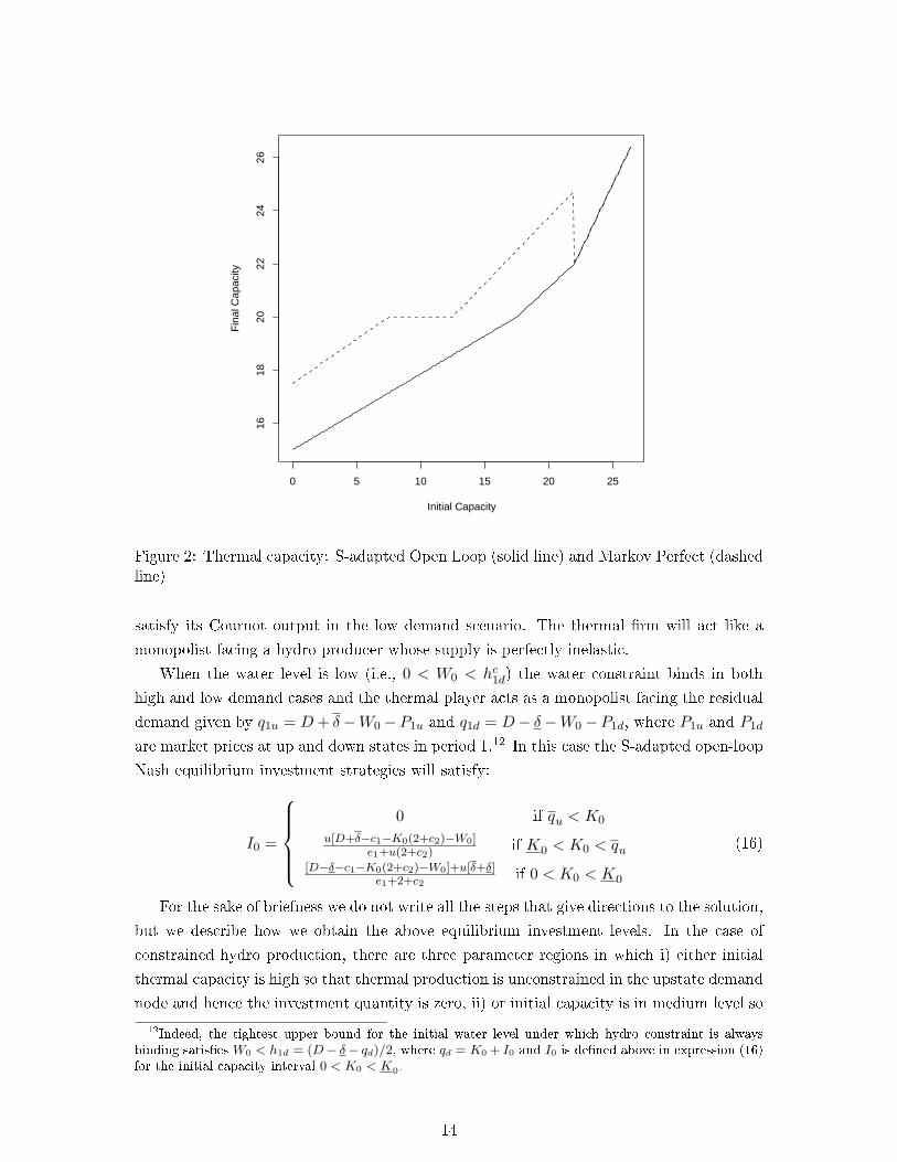
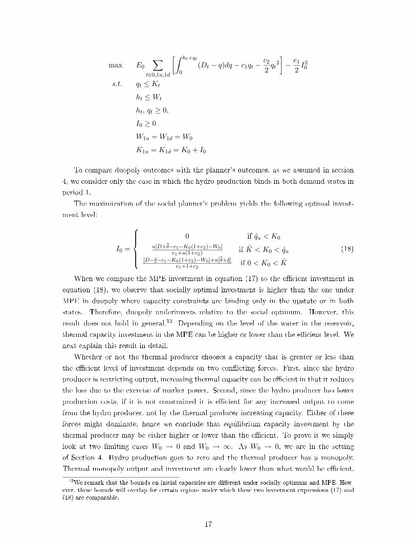
In Figure 2, we plot K1 versus K0 given the equilibrium investments in Figure 1. This

�gure has the same characteristics as that in Figure 1. Period 1 capacities become identical

when there is no investment under both equilibria, otherwise Markov perfect equilibrium

market capacity exceeds that of under the open-loop one.

4 Constrained hydro production

In the previous section, we examined optimum thermal investment behavior when the hydro

player had plenty of water in which its production constraint did not bind at all. Now we

relax this assumption and allow binding water constraints in both periods of the game.

There are two possibilities here: W0 can be very low such that the hydro constraint binds

in both periods, or of an intermediate level where it binds in the high demand state only.

We focus on the former case here.11 This case represents a market structure in which the

thermal player faces a small hydro player that does not have enough reservoir capacity to

11We have analyzed the latter case in which water constraint only binds in the high demand state, howeverthe investment behavior is qualitatively similar to that in Section 3.1, hence we do not report the resultshere.

13

0 5 10 15 20 25

1618

2022

2426

Initial Capacity

Fin

al C

apac

ity

Figure 2: Thermal capacity: S-adapted Open Loop (solid line) and Markov Perfect (dashedline)

satisfy its Cournot output in the low demand scenario. The thermal �rm will act like a

monopolist facing a hydro producer whose supply is perfectly inelastic.

When the water level is low (i.e., 0 < W0 < hc1d) the water constraint binds in both

high and low demand cases and the thermal player acts as a monopolist facing the residual

demand given by q1u = D+ δ−W0 −P1u and q1d = D− δ−W0 −P1d, where P1u and P1d

are market prices at up and down states in period 1.12 In this case the S-adapted open-loop

Nash equilibrium investment strategies will satisfy:

I0 =

0 if qu < K0

u[D+δ−c1−K0(2+c2)−W0]e1+u(2+c2) if K0 < K0 < qu

[D−δ−c1−K0(2+c2)−W0]+u[δ+δ]e1+2+c2

if 0 < K0 < K0

(16)

For the sake of briefness we do not write all the steps that give directions to the solution,

but we describe how we obtain the above equilibrium investment levels. In the case of

constrained hydro production, there are three parameter regions in which i) either initial

thermal capacity is high so that thermal production is unconstrained in the upstate demand

node and hence the investment quantity is zero, ii) or initial capacity is in medium level so

12Indeed, the tightest upper bound for the initial water level under which hydro constraint is alwaysbinding satis�es W0 < h1d = (D− δ− qd)/2, where qd = K0 + I0 and I0 is de�ned above in expression (16)for the initial capacity interval 0 < K0 < K0.

14

that thermal player is constrained when demand is high but unconstrained when demand

is low, and hence investment is positive to cover the demand in upstate, iii) or the initial

thermal capacity is low so that the thermal player is constrained in both up and down

demand states, in which the investment is positive and is being a�ected by both demand

states.

When K0 < K0 < qu the best response functions will satisfy q1u = K0 + I0, h1u = W0,

q1d < q1u, and h1d = W0 in period 1 up and down states for both players. The optimum

investment satis�es I0 = a1u/e1, in which a1u = u[D+ δ− 2q1u−h1u− c2q1u− c1]. Solvingit for investment yields the above equilibrium level. When 0 < K0 < K0, the equilibrium

output levels are q1u = K0 + I0 = q1d, h1u = W0 = h1d, the equilibrium investment

satis�es I0 = (a1u + a1d)/e1, in which a1u = u[D + δ − 2q1u − h1u − c2q1u − c1] and

a1d = (1 − u)[D − δ − 2q1d − h1d − c2q1d − c1]. Solving it for the investment gives the

above result. Clearly, when the initial capacity is high, that is qu < K0, the thermal player

does not invest. Note that the lower bound of initial capacity under which the thermal

player does not invest satis�es qu = (D+ δ− c1 −W0)/(2 + c2), which is the best response

function of thermal player in the upstate demand when the rival hydro player dumps all of

its available capacity into the market.

Next we characterize investment under the Markov perfect equilibrium when the water

level is low. In this case the Markov perfect Nash equilibrium investment strategies are

similar to the one described in Proposition 2 and will satisfy:

I0 =

0 if qu < K0

u[D+δ−c1−K0(2+c2)−W0]e1+u(2+c2) if K ′0 < K0 < qu

[D−δ−c1−K0(2+c2)−W0]+u[δ+δ]e1+2+c2

if 0 < K0 < K ′0

(17)

We calculate the equilibrium investments under the Markov perfect structure as follows:

1. In period 1 at the upstate demand the thermal best response function is q1u = (D +δ − c1 − h1u)/(2 + c2). Since the water level is low the hydro player will produce at

the available water level, which is W0, then the best response quantity for thermal

player becomes q1u = (D + δ − c1 −W0)/(2 + c2). Denote this quantity qu. Clearlywhen qu < K0 is satis�ed upstate capacity constraint is non-binding and hence the

investment quantity is zero.

2. When only upstate thermal constraint is binding the optimum investment satis�es

−e1I0 + u[D + δ − h1u(K1)− 2K1 −K1h

′1u(K1)− c1 − c2K1

]= 0. The equilibrium

outputs in the upstate become h1u = W0 and q1u = K0 + I0, and h′1u(K1) = 0. Plug-

ging these quantities into the above equality and simplifying, we obtain the optimal

investment described above for K ′0 < K0 < qu. The value of lower bound K′0 can be

obtained similar to the one obtained in proposition 2: it will satisfy the property that

downstate production is interior.

3. When the initial thermal capacity is �low�, that is 0 < K0 < K ′0, both upstate and

downstate thermal production constraints do bind. In that case optimum investment

15

satis�es,

−e1I0 + u[D + δ − h1u(K1)− 2K1 −K1h

′1u(K1)− c1 − c2K1

](1− u)

[D − δ − h1d(K1)− 2K1 −K1h

′1d(K1)− c1 − c2K1

]= 0 ,

in which the optimum outputs are h1u = W0, q1u = K0 + I0 = q1d, and h1d = W0,

and also h′1u(K1) = 0 and h′1d(K1) = 0. Plugging these expressions into the above

expression we obtain the investment level for 0 < K0 < K ′0. The bound K ′0 can be

obtained similar to the one obtained in proposition 2: it will be equal to down state

interior Cournot thermal output minus the above investment level for the interval

0 < K0 < K ′0.

The comparison of the investment expressions (16) and (17) yields the following results.

Whenever the water level is so low that hydro production is constrained all times, we do not

observe any strategic value associated with capacity expansion for the thermal �rm in the

Markov perfect equilibrium, and Markov perfect and S-adapted open-loop equilibria invest-

ment levels coincide. Contrary to the case with unconstrained hydro production, thermal

investment is continuous in the Markov perfect equilibrium. Finally, in both equilibria there

is a capacity region in which the thermal investment is independent of the hydro producer's

capacity and output. Outside of this region there is a negative relationship between thermal

investment and the hydro capacity.

5 Socially Optimal Investment

The results of the previous two sections imply that total output is higher in the Markov

perfect equilibrium than in the open-loop equilibrium (when they di�er). Consequently,

prices are lower when strategic e�ects are allowed for. It is important to note that even

though prices are lower, this does not mean that the Markov perfect equilibrium is neces-

sarily more e�cient. The increased output comes about through ine�cient investment in

the cases where the hydro producer has excess capacity. When the hydro producer is not

operating at capacity clearly it would be e�cient to increase output by increasing hydro

production. In the Markov perfect equilibrium however, the increased output comes about

through increased thermal production that is made possible through a costly investment.

We compute the e�cient level of thermal capacity investment by solving the social

planner's problem which chooses production and investment quantities to maximize the sum

of the expected welfare (the consumer surplus less production and investment costs) subject

to non-negativity and capacity constraints. Since the e�cient level of hydro production

is likely higher than the duopoly producers, we allow for the possiblity that the water

constraint binds for the hydro producer. The planner chooses all hydro and thermal outputs

and thermal investment to solve the following problem:

16

max E0

∑t∈0,1u,1d

[∫ ht+qt

0(Dt − q)dq − c1qt −

c22qt

2

]− e1

2I20

s.t. qt ≤ Kt

ht ≤Wt

ht, qt ≥ 0,

I0 ≥ 0

W1u = W1d = W0

K1u = K1d = K0 + I0

To compare duopoly outcomes with the planner's outcomes, as we assumed in section

4, we consider only the case in which the hydro production binds in both demand states in

period 1.

The maximization of the social planner's problem yields the following optimal invest-

ment level:

I0 =

0 if q̂u < K0

u[D+δ−c1−K0(1+c2)−W0]e1+u(1+c2) if K̂ < K0 < q̂u

[D−δ−c1−K0(1+c2)−W0]+u[δ+δ]e1+1+c2

if 0 < K0 < K̂

(18)

When we compare the MPE investment in equation (17) to the e�cient investment in

equation (18), we observe that socially optimal investment is higher than the one under

MPE in duopoly where capacity constraints are binding only in the upstate or in both

states. Therefore, duopoly underinvests relative to the social optimum. However, this

result does not hold in general.13 Depending on the level of the water in the reservoir,

thermal capacity investment in the MPE can be higher or lower than the e�cient level. We

next explain this result in detail.

Whether or not the thermal producer chooses a capacity that is greater or less than

the e�cient level of investment depends on two con�icting forces. First, since the hydro

producer is restricting output, increasing thermal capacity can be e�cient in that it reduces

the loss due to the exercise of market power. Second, since the hydro producer has lower

production costs, if it is not constrained it is e�cient for any increased output to come

from the hydro producer, not by the thermal producer increasing capacity. Either of these

forces might dominate, hence we conclude that equilibrium capacity investment by the

thermal producer may be either higher or lower than the e�cient. To prove it we simply

look at two limiting cases W0 → 0 and W0 → ∞. As W0 → 0, we are in the setting

of Section 4. Hydro production goes to zero and the thermal producer has a monopoly.

Thermal monopoly output and investment are clearly lower than what would be e�cient.

13We remark that the bounds on initial capacities are di�erent under socially optimum and MPE. How-ever, these bounds will overlap for certain regions under which these two investment expressions (17) and(18) are comparable.

17

At the other extreme, as W0 → ∞, equilibrium investment under duopoly is as we have

described in Propositions 1 and 2 of Section 3, i.e., positive. In this case, the e�cient level

of investment is clearly zero since hydro production can meet all contingencies and we have

over-investment relative to the socially optimal level.

6 Hydro Producer Investing in Thermal Generation

In the previous sections we considered a setting in which each duopolist had one type

of production technology. We now allow the hydro producer to operate both hydro and

thermal facilities and invest in thermal production capacity. We will compare investment

levels in two market structures; hydro monopolist investing in thermal generation versus a

thermal duopolist investing in thermal generation.

The producer's maximization problem is to choose hydro and thermal outputs, and

thermal investment quantity to

max E0

∑t∈0,1u,1d

[(Dt − (ht + qt))(ht + qt)− c1qt −

c22qt

2]− e1

2I20

s.t. qt ≤ Kt

ht ≤Wt

ht, qt ≥ 0

K0, I0 ≥ 0

W1u = W1d = W0

K1u = K1d = K0 + I0

Two types of equilibria emerge depending on the water level: a zero investment equilib-

rium and a positive investment equilibrium in which the equilibrium quantity varies with

the initial thermal capacity level. When the water level, W0, is large the hydro production

constraint does not bind, so equilibrium thermal investment by the hydro player is nil since

investment is costly and it will not be used. However, depending on the level of demand the

hydro player can use thermal units for production even if thermal generators are expensive

to run. When the hydro production constraint is binding the hydro producer may invest

in thermal generation. Next we characterize this investment behavior.

The maximization of the above pro�t function yields the optimum investment quantities

conditional on the available thermal capacity levels (the hydro �rm may start with any

positive thermal capacity at time 0). For the sake of briefness, we do not write the �rst

order conditions again since they are similar to the ones in Section 4. The optimal thermal

investment by the hydro �rm is,

18

Ih0 =

0 if q̄u < K0

u[D+δ−c1−K0(2+c2)−2W0]e1+u(2+c2) if K̄ < K0 < q̄u

[D−δ−c1−K0(2+c2)−2W0]+u[δ+δ]e1+2+c2

if 0 < K0 < K̄

(19)

The levels of this investment function correspond to non-binding thermal capacity con-

straint, only up-state capacity binding, and both up and down states capacities binding,

respectively. Comparing expressions (17) and (19) shows that there is higher thermal in-

vestment by a thermal duopolist than by a hydro monopolist due to the market power

of the monopolist. The di�erence between investment levels, I0 − Ih0 , is zero, or equal touW0/(e1 + u(2 + c2)), or equal to W0/(e1 + 2 + c2). Note that the di�erence between in-

vestment levels is not a function of D, δ, and K0 (demand level, demand shock, and initial

thermal capacity, respectively), and the key variable is the water stock W0. This result

holds true for regimes under which initial capacity bounds overlap in (17) and (19).14 If

this water stock is small (and/or investment cost is very high), in the limit the incumbent

hydro producer could invest the same amount as the thermal generator would invest in

duopoly.

7 Conclusions

Capacity investments in electricity markets is one of the main issues in the restructuring

process to ensure competition and enhance system security of networks. In the presence

of evolving demand, possible supply disruptions, and government incentives, production

capacity investments have occurred in many jurisdictions. In this case a simple but an

interesting question arises: What is the investment behavior when two di�erent technologies

compete in an electricity market? In this regard we have analyzed a duopolistic electricity

market in which hydro and thermal generators compete when two di�erent information

structures may be observed.

We have studied dynamic competition between thermal and hydroelectric producers un-

der demand uncertainty, showing that strategic e�ects result in higher investment in thermal

generating capacity than when open-loop strategies are used. In addition, investment is

a discontinuous function of initial capacity in the Markov perfect equilibrium. However,

this higher investment may be ine�cient. Essentially there are two sources of ine�ciency:

the distortion caused by market power and the distortion caused by the industry using an

ine�cient mix of generating technologies.

In our analysis, in the case of large and unconstrained hydro the thermal investment may

be considered as optimum capacity chosen by entry of potential thermal producer. Indeed,

in hydroelectricity dominated jurisdictions (like Quebec, Norway, Brazil, New Zealand)

possible entry is expected by less capital intensive thermal generators. In this case, our

paper presents optimal thermal investment under di�erent behavioral assumptions. In the

14The bounds of initial capacity in expressions (17) and (19) might not be the same. If this occurs, thenthe di�erence between investment levels could depend on initial capacity K0 as well.

19

case of constrained hydro, the capacity expansion could be expected from thermal and

nuclear generators. For instance, in Ontario, Canada hydro facilities are limited due to

environmental and geographic constraints, and capacity investments are done by thermal

generators. The private incentives for investment by the thermal producer di�er from

the social incentives. Part of the private gain associated with investment by the thermal

producer is that they take over some of the sales and revenue of the hydro producer. This

is analogous to the excess entry incentive in Cournot markets.

In this paper we assumed a duopolistic market structure. Even though the quadratic

thermal cost structure may imply aggregate costs by di�erent thermal generation units,

for the sake of simplicity we assumed the same ownership of these thermal generators. We

allowed investment by a thermal generator as well as thermal investment by a hydro genera-

tor. However, in some jurisdictions market capacity could be expanded by constructing new

dams. Also, in some jurisdictions investment in other technologies, like green technologies,

have occurred. For example, capacity investments in wind farms in Germany and Denmark

are becoming an important source of power generation. An interesting extension of our

model would be to incorporate investment in all types of power generation technologies,

which we leave for future research.

References

[1] S.Ambec, J. Doucet. Decentralizing Hydro Power Production. Canadian Journal of

Economics, 36(3):587�607, 2003.

[2] J. Bushnell. A mixed complementarity model of hydrothermal electricity competition

in the western United States. Operations Research, 51(1):80�93, 2003.

[3] J. Bushnell and J. Ishii. Equilibrium model of investment in restructured electricity

markets. mimeo, December 2006.

[4] C. Crampes and M. Moreaux. Water resource and power generation. International

Journal of Industrial Organization, 19(6):975�997, May 2001.

[5] P. Cramton and S. Stoft.The Convergence of Market Designs for Ad-

equate Generating Capacity. Working Paper, 72 pages, April 2006.

http://www.ksg.harvard.edu/hepg/Papers/Cramton_Stoft_0406.pdf

[6] Garcia, A., J. Reitzes, E. Stacchetti. Strategic Pricing When Electricity is Storable.

Journal of Regulatory Economics, 20(3), 223-247, 2001.

[7] A. Garcia and J. Shen. Equilibrium capacity expansion under stochastic demand

growth. Operations Research, forthcoming, 2007.

[8] A. Garcia and E. Stacchetti. Investment dynamics in electricity markets. University

of Virginia, working paper, 2008.

20

[9] T. Genc, S.S. Reynolds, and S. Sen. Dynamic oligopolistic games under uncertainty:

A stochastic programming approach. Journal of Economic Dynamics and Control,

31:55�80, 2007.

[10] T. Genc and S. Sen. An analysis of capacity and price trajectories for the Ontario elec-

tricity market using dynamic Nash equilibrium under uncertainty. Energy Economics,

30(1):173�191, 2008.

[11] A. Haurie, G. Zaccour, and Y. Smeers. Stochastic equilibrium programming for dy-

namic oligopolistic markets. Journal of Optimization Theory and Applications, 66,

1990.

[12] A. Haurie and F. Moresino. S-adapted oligopoly equilibria and approximations in

stochastic variational inequalities. Annals of Operations Research, 114:183�2001, 2002.

[13] F. H. Murphy and Y. Smeers. Generation capacity expansion in imperfectly competi-

tive restructured electricity markets. Operations Research, 53(4):646�661, 2005.

[14] P. Joskow. Competitive Electricity Markets and Investment in New Generating Ca-

pacity. The New Energy Paradigm (Dieter Helm, Editor), Oxford University Press,

2007.

[15] P.O. Pineau and P. Murto. An oligopolistic investment model of the Finnish electricity

market. Annals of Operations Research, 121, 2003.

[16] S. S. Reynolds. Strategic Capital Investment in the American Aluminum Industry.

Journal of Industrial Economics, 4, 1986.

[17] F. Roques, D. Newbery and W. Nuttall. Investment incentives and electricity market

design: the British experience. Review of Network Economics, 4(3), 2005.

[18] T.J. Scott and E.G. Read. Modeling hydro reservoir operation in a deregulated elec-

tricity market. International Transactions in Operational Research, 3(3/4):243�53,

1996.

21