1

Investment Herding by Life Insurers

Chia-Chun Chiang and Greg Niehaus*

Darla Moore School of Business

University of South Carolina

Columbia, SC 29208

July 2015

Do not quote without permission

Abstract:

One of the main arguments for why life insurers are systemically important is that their

investment decisions are highly correlated, i.e., that life insurers herd. We analyze U.S. life

insurers’ investment decisions in corporate bonds from 2002 to 2011 to provide evidence on the

extent to which investment activities are correlated across companies within the life insurance

industry. Based on investment herding measures from the literature, the results are consistent

with life insurers exhibiting herding in corporate bonds, especially in smaller bonds with lower

ratings. Moreover, we find herding is more pronounced among insurers with relatively low risk-

based capital ratios. While we find evidence of investment herding among life insurers, we do

not find evidence indicating that this behavior is likely to be destabilizing to bond markets.

Acknowledgments: The authors appreciate the helpful comments from Jean Helwege, Ashleigh

Poindexter, Eric Powers, and Herman Saheruddin.

1

Investment Herding by Life Insurers

1. Introduction

Academics, insurance professionals, and regulators continue to debate whether traditional

insurance activities of insurers are a source of systemic risk.1 For example, the Financial

Stability Oversight Council (FSOC) in 2014 designated MetLife as a systemically important

financial institution (SIFI), despite objections from Metlife and other commentators (see e.g.,

Wallison, 2014). One of the main arguments for why life insurers are a source of systemic risk is

that life insurers invest a huge amount of funds in financial securities (especially bonds) and that

their trading activity is correlated within the industry, i.e., life insurers herd. As a consequence,

life insurers have the potential to disrupt financial markets and either cause or exacerbate a

systemic event. 2

Schwarcz and Schwarcz (2014) forcefully make this argument and call for

greater regulation.3

The counter argument is that even though U.S. life insurers invest over $2.5 trillion in

bonds (about 75 percent of their general account assets) and hold about one-third of all U.S.

corporate bonds,4 life insurers are typically buy and hold investors; i.e., their trading activity is

much lower than their holdings. Therefore, life insurers trading activities are unlikely to impact

security prices.5 Also, while there are examples of life insurer investment behavior impacting

security prices, this evidence is for isolated securities, during specific time periods, and by a

1 Many commentators acknowledge that non-traditional activities, such as trading credit default swaps, could cause

insurance groups to be systemically important (see e.g., Cummins and Weiss, 2014 and Harrington, 2009). 2 There are other arguments for how insurers could contribute to systemic risk, including concerns about an

insolvency of a one insurer reducing confidence in the ability of other insurers to make good on their promises,

which in turn could cause policyholder runs and cause insurers to liquidate assets quickly and at fire sale prices. See

e.g., Fenn and Cole (1994). Cummins and Weiss (2014) focus on whether reinsurance activities contribute to

systemic risk. 3 On the other side of the spectrum from those who argue that life insurers contribute to systemic risk, Vaughan

(2012) argues that the life insurance industry provides a stabilizing force in financial markets during times of crisis.

This would occur, for example, if during liquidity shocks that induce fire sales from other institutions, insurers

maintain their positions and could even potentially step in on the buy side and help stabilize markets. 4 See McMenamin, et al. (2013) and Campbell and Taksler (2003).

5 Counter arguments to this argument is that trading in corporate bonds is relatively thin overall, and so even a

relatively small amount of trading compared to holdings can potentially impact prices. In addition, a major event

(e.g., a run on life insurers) could cause life insurers to have to liquidate assets quickly.

2

subset of insurers (see the literature discussed in the next section). Currently, there is little

research that focuses on the extent to which life insurers’ investment decisions are correlated

across firms. The purpose of this paper is to fill this gap.

Conceptually, there are several reasons that one might expect herding behavior to exist

among life insurers. First, life insurers face common accounting and regulatory rules.6 As a

result, one might expect insurers to respond in similar ways (buy or sell the same securities) to

changes in these institutional rules and to changes in how a security is treated under these rules.

As an example of the latter situation, a downgrade of a security can increase its risk-based capital

requirement, which in turn could provide incentives for insurers to sell the security. Second,

insurers’ financial condition and future prospects are likely to be impacted in similar ways by

general economic information (such as changes in interest rates and credit spreads) and to

information about the value of specific types of securities. Consequently, insurers might be

expected to adjust their portfolios in similar ways in response to economic information. The

third explanation for herding is referred to as the information cascades theory; it predicts that

company fund managers infer the value of securities from the trades of other fund managers,

which in turn leads fund managers to mimic other fund managers’ trades (Bikhchandani et al.,

1992). Fourth, the literature on how the labor market learns about the ability of fund managers

implies that fund managers will be concerned about poor performance when other funds have

good performance. To avoid this outcome, fund managers will mimic each other (Scharfstein

and Stein, 1990).

To investigate whether life insurers’ corporate bond investment decisions exhibit herding

behavior over the 2002-2011 time period, we calculate herding measures developed by

Lakonishok, et al. (1992). These metrics indicate the extent to which insurers tend to buy the

same securities or sell the same securities within a given time interval. As is common in the

herding literature, we use quarterly time intervals. Our evidence is strongly consistent with life

6 It is also worth noting that often these rules differ from those that apply to other financial institutions, which makes

an analysis of life insurers as a group of interest.

3

insurer herding. The overall herding measure for individual corporate bonds is 9.5 percent on

average, which indicates that on average life insurers are about 9.5 percent more likely to be on

the same side of the market for individual bonds (either on the buy or sell side) than would be

expected if their buy versus sell decisions were independent. We also calculate the buy herding

and sell herding measures, as proposed by Wermers (1999). The overall buy and sell herding

measures for individual corporate bonds have an average value of 9.8 and 9.2 percent,

respectively, indicating that the herding by life insurers is not concentrated on one side of the

market.

We also examine how the herding measures vary with bond and insurer characteristics.

We find that herding by life insurers is greater in smaller bonds and lower rated bonds. This

evidence is consistent with herding being more likely when there is greater asymmetric

information about the bond’s value, which is consistent with the information cascades theory of

herding (Bikhchandani et al., 1992).7 Regarding insurer characteristics, we find that herding

behavior is greater among insurers that have relatively low risk-based capital ratios on average.

Moreover, the relation between herding and risk-based capital ratios is concentrated on the sell

side of the market. These findings are consistent with life insurers with relatively low risk-based

capital selling downgraded bonds around the same time.

Of course, correlated trading does not necessarily imply that life insurers contribute to

systemic risk. While definitive evidence on whether the correlated trading of life insurers is

stabilizing or destabilizing to the bond market is difficult to develop, there are conditions under

which correlated trading is more likely to be stabilizing or destabilizing. We therefore provide

evidence on whether these conditions are present when insurers exhibit herding behavior.

Correlated trading by life insurers is more likely to be destabilizing if the correlated trading is

7 Our results with respect to the impact of bond characteristics on herding by life insurers are similar to those of Cai

et al. (2012), who examine determinants of herding by pension funds, mutual funds, and insurance companies (both

property-liability and life) combined. Our study differs from Cai et al. (2012) in several respects. We only analyze

life insurers; whereas, they do not separately analyze insurers except for reporting the average herding measures by

institutional type. Our sample period, is from 2002-2011 and includes the financial crisis; whereas they examine

2003-2008. We use transaction data; whereas, Cai et al. use quarterly holding data. Finally, we investigate the

impact of insurer characteristics on herding.

4

pro-cyclical, i.e., insurers tend to buy when prices are increasing and sell when prices are

decreasing. In this case, insurer trading activity can exacerbate price movements away from

fundamental values (see Bank of England, 2014). The opposite pattern would be consistent with

insurers’ correlated trading being counter-cyclical, in which case insurer herding is more likely

to provide a stabilizing influence on bond markets (Vaughn, 2012).

We provide two types of evidence on whether insurers’ trading is pro- or counter-

cyclical. In panel regression analysis of herding measures, we find that neither buy nor sell

herding measures are significantly related to past abnormal returns, suggesting that herding is

neither pro- nor counter-cyclical. Using a different methodology, we analyze the abnormal

returns on portfolios of bonds that are selected to have the largest buy and sell herding measures.

We do not find that these portfolios have average abnormal returns different from zero in the 90

days prior to the herding behavior. Thus, the evidence does not suggest that herding is pro-

cyclical, i.e., the evidence does not indicate that herding is likely to be a destabilizing force on

the bond market.

We also examine returns in the quarter during and the quarter subsequent to the herding

behavior in an effort to examine whether there is evidence of herding impacting bond prices. We

find little evidence that herding by life insurers is associated with abnormal returns in either the

quarter in which the herding behavior takes place or in the subsequent quarter. Thus, herding

behavior of life insurers does not appear to have a significant impact on the bond market.

The paper proceeds as follows. In the next section, we review the literature on herding

and the investment decisions of life insurers. The methodology and data are presented in

sections 3 and 4. We present descriptive results on how herding varies with bond characteristics,

insurer characteristics, and time in Section 5. Panel regression analysis of herding measures are

presented in Section 6, followed by the analysis of portfolio returns in Section 7. Some

robustness checks are discussed in Section 8. A short summary concludes the paper.

5

2. Related Literature

2.1 Theories of Herding and Predictions

There are a number of explanations for why institutional investors might exhibit herding

behavior. Institutional factors, such as accounting rules or risk-based capital rules, can cause

insurers to trade in similar patterns. Also, if insurers receive the same information at the same

time about the value of a bond, then they are likely to transact in the same way (see Froot et al.,

1992). Since insurers operating is similar markets and insurers of similar size, capitalization, and

profitability are likely to be impacted similarly by economic information as well as by changes in

regulatory or accounting policies, we examine the extent to which herding is related to these

insurer characteristics.8 In addition, since insurers are likely to respond to bonds with particular

characteristics, in similar ways, we examine whether insurer herding is related to bond

characteristics, such as the bond’s ratings and whether it was recently downgraded.

The information cascade theory of herding posits that some institutions infer information

from the trades of other institutions and therefore mimic the trading of other institutions

(Bikhchandani et al., 1992). Assuming information about securities issued by small companies

is noisier than that of large companies, investors would be more likely to infer information from

other institutional investors about the value of small company securities compared to large

company securities (see Wermers, 1999 and Sias, 2004). According to this explanation, herding

would be most pronounced in bonds of smaller companies.

The information cascade explanation requires that institutions can observe the trading of

other institutions. Cai, et al. (2012) present interesting evidence on this issue by examining an

exogenous change in the extent to which trading information is revealed to other market

participants. Over several phase-in periods between 2002-2005, the Financial Industry

Regulatory Authority (FINRA) required that trade information in the corporate bond market be

8 Understanding the types of insurers that herd is relevant to identifying insurers that contribute to and/or are

exposed to systemic risk. Evidence from Weiss and Muhlnickel (2013) indicates that an insurer’s contribution to

systemic risk is largely explained by insurer size; whereas, an insurer’s exposure to systemic risk is explained by

size, the proportion of net revenue earned from investment activities, and proportion of non-policyholder liabilities

to total liabilities.

6

made public in real time.9 Using a difference-in-difference methodology, Cai et al. (2012) show

that herding increases in bonds that were subject to the final phase-in period. Their findings are

consistent with increased dissemination of trading information increasing the likelihood of

mimicking behavior and increasing the likelihood of information cascades. Because of these

institutional changes in the corporate bond market and because of changes in economic

conditions (e.g., the financial crisis) during our sample period, we incorporate fixed quarter

effects in our analysis.

Another explanation for institutional herding arises from managerial agency problems.

Scharfstein and Stein (1990) show that if managers’ performance across firms is influenced by

common factors and that managers care about their reputations for being a good manager, then

the labor market will assess a given manager’s performance conditional on the performance of

other managers. This, in turn, induces a fund manager to mimic other fund managers so that

he/she does not “standout” from the group if performance is poor.10

Cross-sectional predictions

from this framework would relate to managerial-level information, such as manager

compensation, age, and experience. Unfortunately, we do not have this type of information.

2.2 Empirical Evidence on Herding in Equity Markets

The vast majority of the literature on institutional herding examines equity markets. The

one exception is Cai et al. (2012), which we discuss further as we present our results below.11

The remainder of this section summarizes the evidence from equity markets. The summary is

divided in two parts: (1) evidence on herding, and (2) evidence on the relation between herding

and prior returns, contemporaneous returns, and subsequent returns.

9 On July 1, 2002, FINRA required real-time dissemination of a small number of bonds (Phase 1). In March and

April of 2003, the list was expanded to over 5,000 bonds (Phase 2). Finally, on October 4, 2004 and February 7,

2005 all over-the-counter bonds except Rule-144A bonds were required to reveal real-time trading information

(Phase 3). 10

Dasgupta et al. (2011) build on this idea in their model of the price impact of herding. 11

In addition to institutional herding, there are also studies examining herding by individual investors. See for

example, Dorn et al. (2008), who examine retail clients of a large German discount broker, Barber, et al. (2009b),

who examine clients of two U.S. discount brokers, and Feng and Seasholes (2004), who examine Chinese investors.

7

Lakonishok, et al. (1992) introduced the herding measures that we use and that most of

the herding literature uses. They find some evidence that pension funds herd over quarterly

periods, although the herding is not strong. Wermers (1999) finds essentially the same results

using data on mutual funds. Instead of looking for herding within a quarter, Sias (2004)

examines whether herding occurs across quarters. Consistent with institutional herding, Sias

(2004) finds that institutional buying in one quarter is correlated with institutional buying in the

prior quarter. In other words, herding is persistent from one period to the next. Dasgupta et al.

(2011) also document the persistence of herding behavior.

A number of papers have examined the relationship between herding and the returns

earned during the period prior to the herding period, the herding period, and the period

subsequent to the herding period. Although there is some variation across the studies, Grinblatt

et al. (1995), Wermers (1999), and Nofsinger and Sias (1999) find that positive (negative) stock

returns are associated with institutional buy (sell) herding in the period prior, during, and

subsequent to when the herding takes place. Sias (2004) finds that herding is not positively

associated with prior period returns once he controls for prior period herding. Dasgupta et al.

(2011) also show that persistent herding is negatively correlated with long horizon returns. That

is, buy (sell) herding is associated with negative (positive) abnormal returns over the subsequent

two years. Gutierrez and Kelly (2009) document similar results.

2.3 Investment Decisions of Insurers

Recent literature on life insurer investment decisions indicates that insurers with specific

characteristics change their investments activities in response to changes in economic or

regulatory conditions during specific periods of time. While these papers do not explicitly

examine herding, the evidence indicates that a specific set of insurers are buying or selling the

same type of security at the same time, consistent with herding behavior.

Insurers “Reach” for Yield. Insurers “reaching for yield” means that insurers exhibit a

preference for securities that have higher yields within a rating category. Consistent with this

8

preference, Merrill, et al. (2014a) show that large life insurers that had a relatively high

proportion of liabilities from deferred annuities with interest rate guarantees shifted assets out of

AAA rated corporate bonds and into AAA rated asset backed securities (ABS) over the 2003 to

2007 period. The ABS securities had yields of about 40 basis points higher than AAA rated

corporate bonds. They suggest that this behavior is consistent with these insurers trying to

replenish capital after having suffered capital losses due to lower interest rates during this time

period.

Also consistent with insurers “reaching for yield,” Becker and Ivashina (2013) show that

prior to the financial crisis life insurers with relatively low capital were more likely to purchase

corporate bonds that had higher promised yields within their NAIC rating category relative to

mutual funds and pension funds. They show that these higher yielding bonds did not have higher

average returns than comparable bonds. Thus, it appears that these insurers were trying to boost

reported earnings (which are based on promised yields) and thus reported capital, without

increasing risk-based capital requirements.

Changes in RBC Rules change Insurers’ Investments in MBS. Becker and Opp (2014)

and Hanley and Nikolova (2014) show that insurers’ investment decisions changed after the

NAIC lowered the risk-based capital requirements for non-agency residential mortgage backed

securities (RMBS) in 2009 and for non-agency commercial mortgage backed securities (CMBS)

in 2010. Becker and Opp (2014) show that 92.5% of CMBS purchases were investment grade in

the two years prior to the change; whereas, only 47.0% of CMBS purchases were investment

grade in the two years after the change. Hanley and Nikolova (2014) find that insurers had a

lower probability of selling downgraded MBS after the rule change.

Insurers Sell Downgraded Corporate Bonds. Ambrose, et al. (2008) show that insurers

were more likely to sell downgraded bonds than other bonds during the 1995-2006 period, and

Ellul et al. (2011) find that insurers with relatively low capital ratios were more likely to sell

corporate bonds that were downgraded to non-investment grade during the 2001-2005 period

than insurers with higher capital ratios.

9

In addition, Ellul et al. (2011) find that the downgraded bonds that were sold by insurers

exhibited temporary price declines, but prices reverted back to their original levels over the

subsequent nine months. The price pattern is consistent with the hypothesis that insurers’ trading

activity in the downgraded bonds generated price pressure effects due to limited demand for

these securities by other institutions, including other insurers. Ellul et al. (2011) provide

supplementary evidence consistent with the price pressure explanation. However, Ambrose et al.

(2011) provide evidence that the price drop observed for downgraded bonds is due to the

downgrade providing information to the market of a lower fundamental value for the bonds, not

due to insurers’ trading causing price pressure effects.12

Downgrades of Asset Backed Securities. During the financial crisis, a number of asset

backed securities (ABS) were downgraded, which would lower risk-based capital ratios if

insurers continued to hold the downgraded ABS. Consequently, one might expect insurers to sell

these securities and put the proceeds in investment grade securities. There is, however, an

additional consideration that arises because of the accounting for these securities. Whereas

property-liability insurers are required to report securities with NAIC designations 3, 4, 5, or 6 at

lower of amortized cost and fair value, life insurers are only required to report securities with an

NAIC designation of 6 at lower of amortized cost and fair value. Consequently, following a

downgrade that pushes an ABS into a lower NAIC designation (other than category 6), life

insurers and property-liability insurers face different tradeoffs. Life insurers, especially those

that are poorly capitalized, have a greater incentive to hold downgraded ABS than property-

liability insurers. This is because holding the securities has no effect on the numerator of the

risk-based capital ratio for life insurers, whereas, holding the securities would lower the

numerator for property-liability insurers.

12

The key feature of Ambrose et al. (2011) analysis is that they separately examine bond downgrades that are

associated with stock price declines at the downgrade announcement from downgrades that are not associated with

stock price declines at the downgrade announcement. Ellul et al. (2011) also perform a similar analysis and find

similar results.

10

Ellul et al. (2014) examine the trading of life insurers compared to property-liability

insurers during the financial crisis and show that life insurers with relatively low capital ratios

tended to hold the downgraded ABS compared to property-liability insurers, which tended to sell

these securities. Instead, life insurers were more likely to sell corporate bonds with capital gains,

which bolstered their capital ratios because these bonds were previously reported at historical

cost or amortized value.13

Merrill, et al. (2014) examine the prices at which insurers transacted in RMBS that were

downgraded sufficiently to cross a NAIC rating category between 2007 and 2009. Their

evidence is consistent with insurers that experienced operating losses and subject to fair value

accounting having an incentive to sell downgraded RMBS at fire sale prices. Moreover, they

show that the RMBS sold at lower prices experienced the largest price reversals following the

crisis, after controlling for fundamentals.

Summary. Existing evidence on life insurer investment decisions provides several

reasons why life insurers might exhibit herding behavior. There is evidence that (1) insurers

reach for yield prior to the financial crisis and that this behavior was more likely among insurers

with low capital or those that experienced negative shocks to capital, (2) insurers alter their

investment choices following changes in risk-based capital rules, (3) insurers tend to sell

securities that have been downgraded, but less so when the insurers can continue to report the

value of those securities at historical costs, and (4) life insurers sold corporate bonds with capital

gains to boost capital ratios during the financial crisis. Thus, existing evidence suggests that for

specific securities, under specific conditions, insurers with specific characteristics tend to trade in

a consistent pattern. Moreover the consistent trading of insurers appears to impact prices in

some cases. We now examine whether herding behavior by life insurers is evident more

generally in the market for corporate bonds.

13

Ellul et al. (2014) also provide evidence that the corporate bonds with capital gains that were sold by life insurers

underperformed relative to comparable bonds, which is consistent with life insurers’ trading activities impacting

their prices.

11

3. Methodology

We begin by describing the herding measure for a group of investors that was originally

proposed by Lakonishok, et al. (1992). In the following description, the group of investors is a

group of insurers, which could be the entire group of insurers in our sample or a particular subset

of insurers selected based on specific characteristics. Let

#Bi,t = the number of insurers from the group that were net buyers of security i during

time period t.

#Si,t = the number of insurers from the group that were net sellers of security i during

time period t.

Of all of the insurers from the group that transacted in security i, the proportion that were net

buyers is the insurers’ buy ratio for security i:

pi,t = #Bi,t / (#Bi,t + #Si,t ).

The idea is to test whether the insurers’ buy ratio for security i is different than what would be

expected given the purchasing and selling activity of the group across a broader set of securities.

Thus, pi,t is compared to the overall buy ratio during period t, denoted pt, for a class of securities

to which security i belongs. For example, if security i is a corporate bond with an investment

grade rating, then pit could be compared to the overall buy ratio of all investment grade rated

bonds. The overall buy ratio is defined as follows:

pt = ∑ #𝐵𝑖,𝑡𝑖

∑ #𝐵𝑖,𝑡𝑖 + ∑ #𝑆𝑖,𝑡𝑖 .

The absolute difference, | pi,t – pt | , indicates whether the proportion of net buyers of security i

differs from the proportion of net buyers in the class of securities.

If insurers’ buy versus sell decisions were independent and modeled as a binomial

random variable with probability pt, then the expected value of the absolute difference, | pi,t – pt |,

12

would be positive. Consequently, an adjustment factor is subtracted from the absolute difference

to create the herding measure for security i during period t: 14

HMi,t = | pi,t – pt | - AFi,t ,

where

AFi,t = ∑ | pi,t – pt | (Ni,t

j)

Ni,t

j=0 ptj (1 − pt)Ni,t−j

and Ni,t is the number of insurers transacting in security i during period t. As Ni,t increases, the

adjustment factor declines.

Intuitively, a positive value for the herding measure indicates that the group of insurers

tend to trade a particular security in the same direction more than would be expected if their buy

versus sell decisions were independent. By averaging the herding measure over time and/or

securities, we test whether insurers tend to trade in the same direction, i.e., herd. In addition, we

use panel regressions to examine determinants of the herding measure.

Wermers (1999) introduced a buy and a sell herding measure, denoted BHM and SHM,

by conditioning on whether the security had a higher (lower) buy ratio than the average buy

ratio. That is,

BHMit = HMit if pit > 𝑝𝑡 and undefined otherwise,

SHMit = HMit if pit < 𝑝𝑡 and undefined otherwise.

To illustrate, suppose that five securities are in the sample and the deviations of each security’s

buy ratio from the overall average buy ratio (pit – pt) equal -0.3, -0.1, 0.1, 0.2, and 0.3. For

simplicity, assume the adjustment factor for each security is zero, then the following table would

give the herding measures for each of the five bonds and the average herding measures.

14

To illustrate the calculation of the adjustment factor, suppose that there are three insurers transacting in a

particular bond and that the probability of a buy transaction (pt) is ½. Then there are four possible outcomes for the

buy ratio: 0, 1/3, 2/3, and 1. The probabilities of these outcomes are 1/8, 3/8, 3/8, and 1/8, respectively.

Consequently, the expected value of the absolute difference between the buy ratio and ½ equals

{ | 0

3−

1

2 | (3

0) (

1

2)

0

(1

2)

3

+ | 1

3−

1

2 | (3

1) (

1

2)

1

(1

2)

2

+ | 2

3−

1

2 | (3

2) (

1

2)

2

(1

2)

1

+ | 3

3−

1

2 | (3

3) (

1

2)

3

(1

2)

0

} =

(1/16 + 1/16 + 1/16 +1/16) = ¼, which is the adjustment factor.

13

Bond pit - pt HM SHM BHM

1 -0.3 0.3 0.3

2 -0.1 0.1 0.1

3 0.1 0.1 0.1

4 0.2 0.2 0.2

5 0.3 0.3 0.3

Average 0.2 0.2 0.2

The average overall herding measure (HM) for the sample would be 0.2, the average of the

absolute values of the five individual deviations. The average sell herding measure would be

0.2, the average of the absolute values of the two negative deviations; and the average buy

herding measure would be 0.2, the average of the three positive deviations.

4. Data

We examine insurer transactions in individual bonds over quarterly time periods starting

in the fourth quarter of 2002 and ending in the fourth quarter of 2011.15

The data are from

Schedule D, Parts 3, 4, and 5 of insurers’ annual statements, which report information on bonds

that the insurer purchased during the year (Part 3), sold during the year (Part 4), and bought and

sold during the year (Part 5). As reported in Table 1, there are over 5.4 million bond transactions

reported by 1,353 different life insurance companies in 505,654 different bonds issued by 71,434

issuers. For each transaction, the variables reported include cusip, transaction date, type of

purchaser (including non-market counterparties such as matured, transferred, called, etc.), cost,

par value, and market value. After deleting non-market secondary transactions and those

observations without a reported cusip or a transaction date, the number of transactions drops to

just over 3 million and the number of bonds drops to 429,996.16

The transaction data are merged with the Fixed Investment Securities Database (FISD),

which provides bond characteristics, including issuance date, maturity date, amount outstanding,

15

The TRACE data are available starting in the third quarter of 2002. We begin in the fourth quarter of 2002

because there are very few bonds that meet the data requirements in the third quarter. 16

Non-market transactions are defined by the listed counterparty having one of the following titles: maturity, call,

exchange, in-house, pay-down, tax write-off full redemption internal transfer, tender, merged, dividend, basis

spinoff, mortgage, or corporate reorganization.

14

coupon rate, and rating history. We restrict the sample to bonds that (a) have remaining maturity

greater than two quarters (because bonds with remaining maturity less than two quarters will

necessarily leave the insurer’s portfolio over the coming quarter), (b) were issued at least three

quarters prior (to avoid potential new issue effects), (c) have a fixed coupon,17

(d) are corporate

bonds denominated in U.S. dollars (because bond characteristics are missing for most of the

other bonds).18

The number of bonds in the sample drops to 23,634 as a result of this step. The

data are then merged with the Trade Reporting and Compliance Engine (TRACE) data to obtain

liquidity and volume measures (excluding those with absolute daily return greater than 100%),

which reduces the number of bonds to 14,707.

The data are also merged with insurer annual statement data to obtain insurer

characteristics, such as size and capitalization measures. Insurers with missing or negative value

for surplus, total assets, or net premiums written are excluded, which reduces the number of

bonds to 14,650. We impose the restriction that each bond in the sample in a given quarter must

have at least five transactions in the quarter. This gives us 248,020 bond transactions in 6,949

bonds by 906 life insurers. Finally, since most of our analysis will utilize prior quarter bond

returns, we drop observations for which we cannot calculate the prior quarter return. The

resulting sample has 181,512 bond transactions in 5,364 bonds by 890 life insurers. Recall the

herding measures are calculated using all of the transactions by life insurers in a given bond and

quarter. There are 20,766 bond-quarter observations (not tabulated).

In Table 2, we present descriptive statistics for the observations that are used in the

regression analysis. For this table, we treat each transaction as a separate observation. On

average, the bonds transacted have a maturity when issued of 14.1 years, 10.3 years remaining

until maturity, and are 3.8 years old. The average (median) face amount is $94 ($65) million.

Credit Rating takes a value between one and ten, where one indicates the highest rating (AAA)

17

The data do not include information about the formula for variable coupon bonds. 18

This process follows that used by Cai et al. (2012).

15

and ten is the lowest rating (in default).19

The average (median) credit rating is 3.9 (4.0) and 70

percent of the bonds transacted have an investment grade rating (i.e., above BB).

Regarding insurer characteristics, we calculate each insurer’s risk-based capital ratio and

then winsorize at the 1% and 99% levels. The average (median) risk-based capital ratio (RBC) is

8.5 (8.0). The distribution of insurer asset size is skewed with a mean of $39.1 billion and a

median of $28.5 billion. Using 75 percent of premiums written in one line of business as an

indicator of product line focus, 13 percent of insurers focus in life insurance, 39 percent focus in

the annuity business, and 9 percent focus in accident and health insurance.

5. Descriptive Analysis of Herding

Table 3 reports the herding measures for the sample described in Table 2. The average

herding measure (HM) equals 9.5 percent, which is statistically different from zero. This

estimate indicates that life insurers’ tend to buy the same bond or sell the same bond more so

than would be expected if their buy and sell decisions were independent. Also reported in Table

3, the buy herding measure for the overall sample is 9.8 percent and the sell herding measure for

the overall sample is 9.2 percent. These results indicate that the herding behavior of life insurers

19

To calculate a bond’s credit rating, we use the average of the four major credit rating agencies ratings and assign

the bond to a rating category as described in the following Table.

Avg rating of 4 credit rating agencies Credit Rating % of Obs

AAA 1 1.1%

Above AA 2 6.3%

Above A 3 26.4%

Above BBB 4 35.1%

Above BB 5 15.5%

Above B 6 10.5%

Above CCC 7 3.0%

Above CC 8 0.5%

Above C 9 0.3%

Default 10 0.5%

NR&w w 1.0%

16

is not concentrated on the buy or sell side of the market. Instead, both buy and sell decisions are

correlated across life insurers.20

To put these herding measures in perspective, Panel B of Table 3 reports selected results

from the prior literature on herding for other types of institutional investors, securities, and time

periods. Generally, the evidence indicates relatively small herding measures for institutional

investors’ stock transactions (see e.g., Lakonishok et al., 1992 and Wermers, 1999). However,

the evidence on bond transactions by institutional investors by Cai et al. (2012) indicates much

higher herding measures, consistent with our results.

Figures 1 – 3 report herding measures for subsets of bonds based on various bond

characteristics. For these analyses, the expected buy ratio (pt) is the buy ratio for all of the bonds

within the category of bonds being considered, as opposed to the buy ratio for all bonds, as was

used in herding measures reported in Table 3. For example, in Figure 1, which reports the

average herding measure for bonds in four size (amount outstanding) categories, the expected

buy ratio for each size category uses only the bonds within that category.

Figure 1 illustrates that the average herding measures (HM, BHM, and SHM) are highest

for bonds with the lowest amount outstanding (between zero and $20 million) and that the

average herding measures decline as the face value of the bond increases. These results are

consistent with existing studies that institutional herding is significantly greater in small stocks.

One explanation is that small bonds have less public information, and therefore life insurers are

more likely to make decisions based on other insurers’ behavior, consistent with informational

cascades (Bikhchandani et al., 1992).21

20

If the entire sample of 100,304 bonds is used, as opposed to those that went through the various data screens

outlined in Table 1, the herding measures are higher: HM = 16.3 percent, BHM = 11.1 percent, and SHM = 21.5

percent. The higher SHM than BHM is this broader sample is consistent with Cai et al. (2012). 21

We also examined whether herding measures are related to bond maturity. If herding is more likely in securities

with greater information asymmetry and if longer maturity bonds have greater information asymmetry (see Barnea

et al., 1980), then we would expect longer maturity bonds to have higher herding measures. However, we find that

the average herding measure is low for bonds with maturity less than or equal to one year and for bonds with

maturity greater than 20 years compared to bonds with intermediate maturities.

17

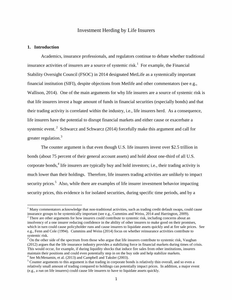
Figure 2 shows that the average herding measures vary little with the Amihud (2002)

liquidity measure. There is, however, a slight U shape in the graph. Cai et al. (2012) find a

similar pattern. They suggest that it results from a trade-off between the benefits of information

based herding and transaction costs. Illiquid bonds are likely to have greater information

asymmetry, thus resulting in greater herding behavior. However, illiquid bonds are more costly

to trade, making the herding strategy less profitable. This tradeoff results in very liquid bonds

being traded because of low transaction cost and very illiquid bonds being traded because of high

private information.

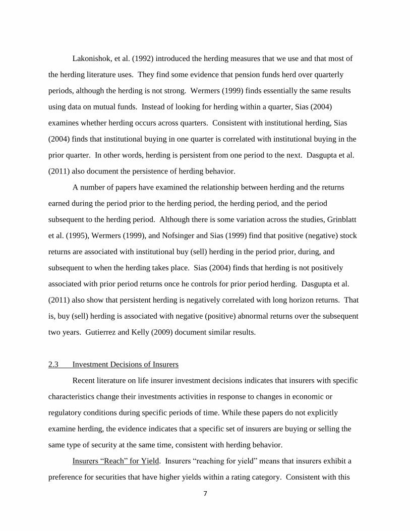
Figure 3 illustrates that the average herding measures are lower for investment grade

compared to non-investment grade bonds. In addition, the average buy herding measure is

higher than the average sell herding measure for non-investment grade bonds. Several factors

could explain this relationship. First, if non-investment grade bonds have greater information

asymmetry, which induce insurers to mimic trades of other insurers, then herding would be

greater in non-investment grade bonds. Second, because of the higher risk-based capital

requirements of non-investment grade bonds, insurers, especially those with lower capital, will

have an incentive to sell bonds that are downgraded from investment grade to non-investment

grade (see Ambrose et al., 2008 and 2012, and Ellul et al., 2011 and 2012). Third, buy herding

could result from financially strong insurers purchasing bonds that have been downgraded and

that are experiencing downward price pressure from other institutions that are selling these

bonds.22

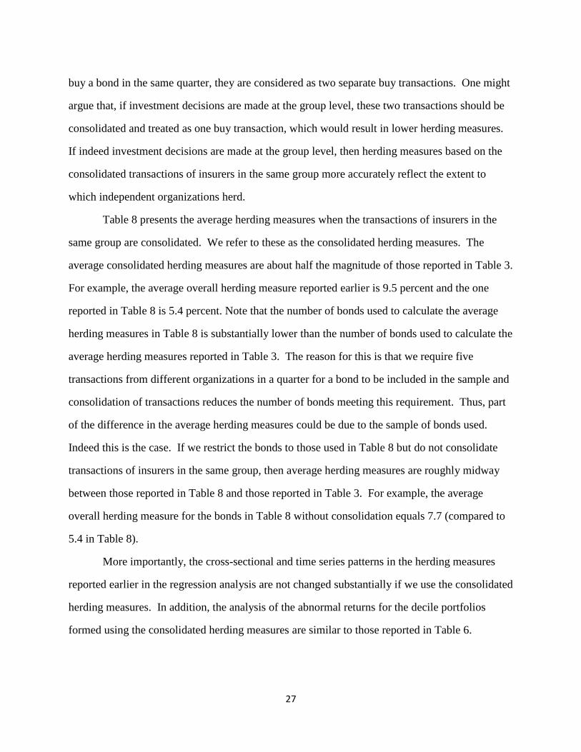
Figure 4 illustrates how the average herding measures vary over time. For this analysis,

the expected buy ratio (pt) is calculated using all of the bonds in the sample, as was done in

Table 3. The average herding measures increase gradually from 2004 through 2009. In 2010

and 2011, the average herding measures return to roughly the same level as before the financial

crisis. Thus, there is some evidence that herding by insurers increased during the financial crisis.

22

See Feng and Seasholes (2012) for related arguments.

18

Figure 5 illustrates the average herding measures based on the average risk-based capital

ratios of the insurers transacting in the bonds. For this analysis, the expected buy ratio is

calculated using all of the bonds traded by the insurers in the risk-based capital category. The

four risk-based capital categories are the quartiles of the average risk-based capital ratios of the

insurers in the sample. Figure 5 indicates that the insurers with the lowest risk-based capital

ratios exhibit the strongest herding behavior.23

Finally, Figure 6 presents the average herding measures for insurers with different

product line focus. For this analysis, the expected buy ratio is calculated using all of the bonds

traded by the insurers with the same product focus. We define an insurer as having a product

line focus in life insurance, annuities, or accident & health insurance if the insurer has 75 percent

of its premium revenue from one of these lines. Otherwise, we categorize the insurer as not

having a focus. Figure 6 indicates that on average the herding measures are higher for insurers

with no focus and with an accident and health focus than for insurers with a life insurance and

annuity focus.

6. Panel Regressions of Herding Measures

We now turn to a panel regression analysis of the bond herding measures. The dependent

variable is either the overall herding measure (HMit), the sell herding measure (SHMit), or the

buy herding measure (BHMit) for bond i during quarter t. The explanatory variables include

Ageit = bond i’s age in years,

AmtOutit = bond i’s average of the logarithm of the amount outstanding during quarter t,

Ratingit = bond i’s average rating score during quarter t,

Liquidityit = bond i’s average Amihud liquidity measure during quarter t,

Upgrit = 1 if bond i is upgraded at least once during quarter t, and 0 otherwise,

23

For Figures 5 and 6, the data are divided into categories by insurer characteristics. Consistent with the

construction of the overall sample, we impose the restriction that there must be five transactions for a given bond in

a given quarter by the insurers in the same category. As a consequence, there are far fewer bond-quarter

observations used in these Figures and the number of observations across the categories in Figure 5 varies even

though the RBC ratios are based on the quartile values.

19

Downgrit = 1 if bond i is downgraded at least once during quarter t, and 0 otherwise,

Invgrit = 1 if bond i’s average rating was above BB in quarter t, and 0 otherwise,

PrRetit = the previous quarter’s abnormal return for bond i,24

Avg. RBCit = average risk-based capital ratio of insurers transacting in bond i during quarter t,

Avg. ROAit = average return on assets of insurers transacting in bond i during quarter t,

Avg LogSizeit = average logarithm of inflation adjusted general account assets of insurers

transacting in bond i during quarter t,

Avg Focus_Lifeit = the average value for insurers transacting in bond i during quarter t of a

dichotomous variable that equals 1 if an insurer’s percentage of premiums written

in life insurance exceeds 75 percent, and zero otherwise.

Avg Focus_Annit = the average value for insurers transacting in bond i during quarter t of a

dichotomous variable that equals 1 if the average percentage of premiums written

in annuity exceeds 75 percent, and zero otherwise.

Avg Focus_AHit = the average value for insurers transacting in bond i during quarter t of a

dichotomous variable that equals 1 if the average percentage of premiums written

in accident & health insurance exceeds 75 percent, and zero otherwise.

The variables can be placed in two categories: (1) bond characteristics and (2) insurer

characteristics. Most of the bond characteristics can be considered control variables. The one

exception is PrRet, the bond’s abnormal return in the previous quarter. A positive (negative)

coefficient on PrRet in the buy herding regression would be consistent with herding being pro-

(counter-) cyclical on the buy side, i.e., insurers buy after the price has increased (decreased). A

positive (negative) coefficient on PrRet in the sell herding measure would be consistent with

24

The previous quarter return is calculated using the 90 days prior to the first date (denoted F) in which an insurer

in the sample transacted in the bond during the quarter and equals (𝑃𝑖,𝐹−1+𝐴𝐼𝑖,𝐹−1)−(𝑃𝑖,𝐹−91+𝐴𝐼𝑖,𝐹−91)+𝐶

(𝑃𝑖,𝐹−91+𝐴𝐼𝑖,𝐹−91)−

𝐼𝑖,𝐹−1−𝐼𝑖,𝐹−91

𝐼𝑖,𝐹−91,

where 𝑃𝑖,𝐹−𝑥 is the bond price on day F-x (x days before first transaction by an insurer in the quarter), AIi,F-x is

accrued interest on day F-x, and C is the coupon payment(s) received. 𝐼𝑖,𝐹−𝑥 is the matching portfolio value x days

before the first transaction date by an insurer in the quarter. We follow Bessembinder, et al. (2009) and construct

matching portfolios (benchmark portfolios) using the Citi US Broad Investment Grade Bond Index and Citi High

Yield Market Index. This approach allows us to classify bonds into five major rating categories (AAA-AA, A, BBB,

BB, CCC), and then segment these categories into intermediate and long-term indices based upon time to maturity,

resulting in 18 matching portfolios. For investment grade bonds, the time to maturity categories are 1 to 3 years, 3

to 7 years, 7 to 10 years, and 10 or more years. For non-investment grade bonds, the categories are 1 to 7 years, 7 to

10 years, and 10 or more years.

20

herding being counter- (pro-) cyclical, i.e., insurers sell after the price has increased (decreased).

We also include bond and quarter fixed effects to control for time-invariant unobservable bond

characteristics and time effects that may affect the herding level.

The panel regression results are reported in Table 4. Regarding bond characteristics, the

multivariate analysis reinforces some of the relationships found in the univariate analysis in

Figures 1 - 4. First, overall herding is greater in smaller bonds, as the coefficient on AmtOutst is

negative and statistically significant in the HM regression. Second, as Rating increases (credit

risk increases), the overall herding measure increases. A one unit increase in Rating (e.g., a drop

from AA to A), increases the herding measure by 0.019 (1.9 percent). However, the regression

analysis of the buy and sell herding measures (columns two and three in Table 4) indicate that

both the size and rating effects are concentrated on the sell side, as the coefficients on the

AmtOutst and Rating are only statistically significant in the sell herding measure (SHM)

regression. Thus, insurer sell herding is more likely with smaller bonds with low ratings.

Investment grade bonds exhibit a significantly lower overall herding measure (HM), even

after controlling for Rating. The estimated coefficient on InvGr indicates that investment grade

bonds have a 0.028 (2.8 percent) lower herding measure on average, controlling for the other

factors. The coefficients on UpGr and DownGr give the estimated impact on herding of a

change in the bond’s rating during the quarter. We do not find a significant effect of upgrades on

buy or sell herding measures. Downgrades, however, are associated with a significant increase

in the sell herding measure and a significant decrease in the buy herding measure. Moreover, the

impact of a downgrade is economically significant, lowering the buy herding measure by 3.5

percent and increasing the sell herding measure by 2.4 percent. There is no relation between

downgrades and the overall herding measure, consistent with impact of downgrades on the buy

side canceling the impact of downgrades on the sell side. These findings are consistent with the

literature that indicates that insurers tend to sell downgraded bonds (Ambrose et al. (2008, 2011)

and Ellul et al. (2011)).

21

The coefficient on the PrRet variable is not statistically significant in any of the

regressions. Thus, we do not find evidence of herding being pro- or counter-cyclical using the

prior quarter abnormal return.

Regarding insurer characteristics, the panel regressions indicate that larger, more

profitable insurers are less likely to engage in herding, especially buy herding. In addition,

insurers with higher risk based capital ratios are less likely to engage in herding, especially sell

herding. A concern with this regression model is that it imposes a linear relation between

herding and the risk-based capital ratio. Differences in risk-based capital ratios are likely to

matter less when risk-based capital ratios are relatively high. Therefore, in Table 5, we report

the results of an alternative specification that replaces the RBC variable with two dichotomous

variables indicating whether the average risk-based capital ratio is less than 7 and between 7 and

9. These cutoffs roughly correspond to the 25th

and 75th

percentile values for RBC.

We only report the results for the insurer characteristics in Table 5, but all of the other

variables are included in the model. The coefficient on the dichotomous variable indicating a

risk based capital ratio less than 7 is positive and statistically significant in the overall herding

measure regression and in the sell herding measure regression. The coefficient estimates are also

economically significant. A low RBC ratio is associated with an increase in the overall herding

measure of 1.2 percent and in the sell herding measure of 1.4 percent. This evidence suggests

that insurers with low risk-based capital ratios are more likely to exhibit herding behavior.

As a robustness check, we re-estimated the regression models with the lagged herding

measure as an additional explanatory variable. This is motivated by Sias (2004) and Dasgupta et

al. (2011), who document persistence in herding behavior in equity markets over time. The

coefficient on the lagged herding measure is positive and statistically significant at the 10 percent

level, consistent with persistence. However, the estimated coefficients on the other explanatory

variables remain roughly the same as those reported in Tables 4 and 5.

22

7. Relation between Herding and Bond Abnormal Returns

We further examine whether life insurer herding is pro-cyclical or counter-cyclical using

a methodology similar to that employed by Barber et al. (2009) and Dorn et al. (2008) in their

studies of equity market herding. This methodology also allows us to examine abnormal bond

returns during and subsequent to life insurer herding behavior, which provides additional

evidence on the impact of life insurer herding on the bond market. Regarding returns during and

subsequent to the herding period, there are at least four possible findings and corresponding

interpretations:

1. Positive (negative) abnormal returns during the quarter in which buy (sell) herding

occurs followed by zero abnormal returns in the subsequent quarter would be

consistent with insurers having better information about the value of bonds and that

their herding incorporates that information into the price of the bonds.

2. Zero abnormal returns during the quarter in which buy (sell) herding occurs followed

by positive (negative) abnormal returns in the subsequent quarter would be consistent

with insurers having better information about the value of bonds, but that their

herding does not impact prices; instead, the information is impounded in prices in the

subsequent quarter.

3. Positive (negative) abnormal returns during the quarter in which buy (sell) herding

occurs followed by negative (positive) abnormal returns in the subsequent quarter

would be consistent with insurer herding causing price pressure, which is relieved in

the subsequent quarter.

4. Zero abnormal returns during the quarter in which buy (sell) herding occurs followed

zero abnormal returns in the subsequent quarter would be consistent with insurer

herding not having an impact on the market.25

25

The lack of impact does not imply that insurers do not have better information about the value of bonds; it could

take longer than the next quarter for the information to be impounded into prices.

23

For each quarter q, we divide all of the bonds in the sample in two categories: (1) those

with a buy ratio greater than the average buy ratio during the quarter and (2) those with a buy

ratio less than the average buy ratio during the quarter. Recall, the bonds in the first category are

used to construct the buy herding measure and those in the second category are used to construct

the sell herding measure. The bonds in the first category are then divided into quintiles (P1 to

P5) based on the magnitude of their buy-herding measures (BHM). Portfolio P1 consists of the

bonds with the highest buy herding measures in each quarter. We repeat the same rank

procedure for bonds with sell-herding measures, creating portfolios P6 to P10, where portfolio

P10 represents the portfolio of bonds with the highest sell herding measures in each quarter.

The first three columns of Table 6 provide descriptive information about the average

number of bonds in each portfolio and the average herding measure (buy herding measure for

portfolios P1-P5 and the sell herding measure for portfolios P6-P10) over the sample period.26

The average herding measure in Portfolio 1 is 33.7 percent and the average herding measure in

Portfolio 10 is 31.0 percent, both of which suggest a substantial degree of herding in the bonds in

these portfolios. Portfolios 2 and 9 have average herding measures of 18.7 percent and 20.0

percent, respectively; these numbers also suggest a high degree of herding in the bonds in these

portfolios. In contrast, portfolios 4, 5, 6, and 7 have herding measures that are negative,

indicating little herding in the bonds in these portfolios.

For each of these 10 portfolios and for each of the 37 quarters, we calculate the equally-

weighted abnormal returns for the quarter before, the quarter of, and the quarter after the

portfolio formation quarter. As described in an earlier footnote, the abnormal returns are

calculated using the matching portfolio methodology in Bessembinder, et al. (2009). For a given

bond and quarter, let F equal the first transaction date by an insurer in the bond and L equal the

last transaction date in the quarter by an insurer in the bond. Then the abnormal return is

26

The average number of bonds in the various portfolios can vary slightly due to the way that ties (bonds with the

same value of the herding measure) are treated.

24

calculated for the time intervals: [F-91,F-1], [F,L], and [L+1,L+91].27

This is repeated for each

bond in the portfolio in the quarter and the resulting values are averaged to calculate the average

abnormal return for the portfolio for that quarter. These quarterly average abnormal returns are

then averaged over the 37 quarters to calculate the overall average abnormal return for each of

the 10 portfolios.28,29

Table 6 reports the overall average abnormal returns for each of the 10 portfolios. We

focus on the portfolios with the largest herding measures: P1, P2, P9, and P10. Consider first the

abnormal returns in the quarter prior to the portfolio formation. The -0.9 percent abnormal

return for P1 is large in economic terms and is consistent with counter-cyclical buy herding.

However, it is not statistically significant. The bonds in portfolio P2 are not associated with a

significant average abnormal return in the quarter prior to the buy herding. Similarly, the bonds

with the most extreme sell herding measures (P10) are not associated with a significant average

abnormal return in the prior quarter. However, the bonds in P9 on average performed poorly in

the prior quarter as they earned a -0.7 percent abnormal return, which is significantly different

from zero at the 10 percent level. The results for P9 are consistent with pro-cyclical herding (sell

herding following price declines). Thus, the results for the prior quarter abnormal returns

provide some evidence of pro-cyclical and some evidence of counter-cyclical herding by life

insurers, but neither piece of evidence is strong.

For the quarter in which the portfolios are formed, the buy herding portfolios all have

negative abnormal returns, but none of the abnormal returns is significantly different from zero.

27

As is well-known, the secondary corporate bond market in general exhibits thin trading, i.e., many bonds do not

trade on a daily basis. In addition, not all transactions are reported in TRACE (our source of bond price

information). Consequently, when no transaction is reported in the TRACE data for one of the days of interest to us,

we use the nearest prior transaction price in TRACE. Only about seven percent of the days for which we seek a

price have a transaction on that day. In 49 percent of the other days, a transaction price is found in the prior 30 days,

but in about 51 percent of the other cases, we need to go back more than 30 days to find a transaction price. 28

The appendix describes the results of an alternative method that calculates average abnormal returns over the 90

days prior to each trade in the portfolio formation quarter and 90 days subsequent to each trade of each quarter. 29

The statistical significance of the overall average abnormal returns is based on the assumption that the portfolio

average abnormal return in one quarter is independent of the average abnormal return in the other quarters. An

alternative assumption would be to treat the abnormal returns of each individual transaction as being independent.

Because the latter approach would ignore the clustering of event windows in a given calendar period, we report

significance using the former approach. The appendix presents the results using the latter approach.

25

Similarly, none of the abnormal returns for the sell herding portfolios is significantly different

from zero. Finally, consider the quarter subsequent to the portfolio formation quarter. Neither of

the extreme buy herding portfolios (P1 and P2) and neither of the extreme sell herding portfolios

(P10 and P9) exhibit abnormal returns. In summary, the results regarding abnormal returns in

the quarter in which herding occurs and in the quarter after herding occurs do not indicate that

insurer herding has a consistent impact on the bond prices.

8. Robustness Checks

Taking into Account the Amount Traded. The herding measures used in the paper take

into account the number of trades, but not the size of the trades. Thus, a $50,000 buy transaction

is treated the same as a $5 million buy transaction. To incorporate the size of the transaction, we

utilize a herding measure used by Oehler and Chao (2000), which takes into account the volume

of buy trades and sell trades by insurers. The herding measures based on volume for bond i in

quarter t equals the absolute value of the difference between the amount purchased by insurers

and the amount sold by insurers as a proportion of the total amount transacted by insurers:

| Amount Purchasedit – Amount Soldit | / [ Amount Purchasedit + Amount Soldit ].

In addition to taking into account the amount sold, the herding measure based on volume differs

from the herding measures based on the number of trades in that it does not subtract a benchmark

measure of insurer buy versus sell volume in the bond market. Thus, unlike the earlier measures,

this is not a measure of insurer trading in a particular bond relative to insurer trading in the bond

market.

To form portfolios of bonds with common values for the herding measure based on

volume, we first consider the bonds for which insurers’ buy volume is greater than their sell

volume. We place these bonds info five portfolios using on the herding measured based on

volume. Portfolio P1 has the bonds with the highest herding measures based on volume and

portfolio P5 has the bonds with the lowest measures. We then do the same process for the bonds

26

with insurer sell volume greater than buy volume. Portfolio P10 has the highest herding measure

based on volume and portfolio P6 has the bonds with the lowest measures.

Table 7 presents the average values of the herding measure based on volume for each of

the portfolios and the average abnormal returns in the quarter prior to, during, and subsequent to

portfolio formation. As with the earlier analysis, we focus on portfolios P1, P2, P9, and P10.

The portfolio with the bonds with the largest buy herding measures based on volume, P1, has a -

1.2 percent abnormal return in the quarter prior to portfolio formation and it is statistically

different from zero at the 5 percent level. This is consistent with counter-cyclical herding.

Portfolio P9, which has the second largest sell herding measure based on volume, has a

statistically and economically significant -1.1 percent abnormal return in the quarter prior to

portfolio formation, which is consistent with pro-cyclical herding. Thus, there is some evidence

that insurers are buying bonds that have recently performed poorly and also selling bonds that

have recently performed poorly. These results are similar to those presented earlier with the

herding measures based on trades.

Now consider the quarter during and after portfolio formation. One difference between

the results in Table 7 and the earlier results is that portfolio P9 has negative and statistically

significant abnormal returns during the portfolio formation quarter, which is consistent with

insurer sell herding impacting the market price.30

Consistent with the earlier analysis, none of

the other extreme herding portfolios (P1, P2, and P10) exhibit significant abnormal returns

during the herding quarter or subsequent to the herding quarter. Overall (and consistent with the

earlier analysis), the results do not provide strong evidence that insurer trading has a consistent

impact on the bond market.

Group versus Company Herding Measures. The herding measures reported throughout

the paper are calculated using company level data. Thus, if two companies in the same group

30

Although we do not focus attention on Portfolio P8, it is worth noting that it also has negative and statistically

significant abnormal returns during the portfolio formation quarter. The negative abnormal returns continue in the

subsequent quarter for P8, which is consistent with insurers having information about the value of the bonds that is

slowly impounded into the price and inconsistent with the price pressure explanation.

27

buy a bond in the same quarter, they are considered as two separate buy transactions. One might

argue that, if investment decisions are made at the group level, these two transactions should be

consolidated and treated as one buy transaction, which would result in lower herding measures.

If indeed investment decisions are made at the group level, then herding measures based on the

consolidated transactions of insurers in the same group more accurately reflect the extent to

which independent organizations herd.

Table 8 presents the average herding measures when the transactions of insurers in the

same group are consolidated. We refer to these as the consolidated herding measures. The

average consolidated herding measures are about half the magnitude of those reported in Table 3.

For example, the average overall herding measure reported earlier is 9.5 percent and the one

reported in Table 8 is 5.4 percent. Note that the number of bonds used to calculate the average

herding measures in Table 8 is substantially lower than the number of bonds used to calculate the

average herding measures reported in Table 3. The reason for this is that we require five

transactions from different organizations in a quarter for a bond to be included in the sample and

consolidation of transactions reduces the number of bonds meeting this requirement. Thus, part

of the difference in the average herding measures could be due to the sample of bonds used.

Indeed this is the case. If we restrict the bonds to those used in Table 8 but do not consolidate

transactions of insurers in the same group, then average herding measures are roughly midway

between those reported in Table 8 and those reported in Table 3. For example, the average

overall herding measure for the bonds in Table 8 without consolidation equals 7.7 (compared to

5.4 in Table 8).

More importantly, the cross-sectional and time series patterns in the herding measures

reported earlier in the regression analysis are not changed substantially if we use the consolidated

herding measures. In addition, the analysis of the abnormal returns for the decile portfolios

formed using the consolidated herding measures are similar to those reported in Table 6.

28

9. Summary

Using traditional measures of investment herding (correlated trading) among institutions,

we find that U.S. life insurers’ investment decisions in corporate bonds are consistent with

herding behavior. That is, life insurers tend to be on the same side of the market (either buying

or selling) in individual corporate bonds than would be expected if their investment decisions

were independent of each other. This behavior is more pronounced in smaller bonds and lower

rated bonds, and is more pronounced among insurers with relatively low risk-based capital ratios.

Correlated trading among life insurers is one of the channels that has been put forth for

why life insurers could contribute to systemic risk (see Schwarcz and Schwarcz, 2014). The

evidence presented here therefore lends credence to the argument that life insurers’ investment

activities could be a source of systemic risk. However, correlated trading does not imply that life

insurers’ investment decisions have an impact on market prices. Thus, we also examine the

relationship between herding behavior and both previous and subsequent abnormal returns. We

do not find strong associations between herding behavior and abnormal returns in the quarter

before, during, or after life insurer herding behavior. In other words, there is little evidence that

life insurer herding is responsive to the market or impacts the market. This evidence lessens

concerns about herding behavior of life insurers contributing to systemic risk.

29

References

Ambrose, Brent, Kelly Cai, and Jean Helwege, 2008, Forced Selling of Fallen Angels, Journal of

Fixed Income 19, 72-85.

Ambrose, Brent, Kelly Cai, and Jean Helwege, 2012, Fallen Angels and Price Pressure, Journal of

Fixed Income 21, 74-86.

Acharya, V, J. Biggs, M. Richardson, and S. Ryan, 2009, On the Financial Regulation of Insurance

Companies, working paper, NYU Stern School of Business.

Amihud, Yakov, 2002, Illiquidity and stock Returns: Cross-sectional and Time Series Effects,

Journal of Financial Markets 5, 31-56.

Balcuh, F., S. Mutenga, and C. Parson, 2011, Insurance, Systemic Risk and the Financial Crisis, The

Geneva Papers 36, 126-163.

Bank of England, 2014, Procyclicality and structural trends in investment allocation by insurance

companies and pension funds, Discussion Paper by the Bank of England and the Procyclicality

Working Group, July 2014

Barber, Brad, Terrance Odean, and Ning Zhu, 2009a, Do Retail Investors Move Markets, Review of

Financial Studies 22, 151-186.

Barber, Brad, Terrance Odean, and Ning Zhu, 2009b, Systematic Noise, Journal of Financial

Markets 12, 547-569.

Becker, Bo, and Victoria Ivashina (2013), “Reaching For Yield in the Bond Market”, forthcoming,

Journal of Finance.

Becker, Bo and Marcus Opp, 2014, Regulatory Reform and Risk Taking, working paper, Stockholm

School of Economics.

Bessembinder, Hendrick, Kathleen M. Kahle, William F. Maxwell and Danielle Xu, 2009,

Measuring Abnormal Bond Performance, The Review of Financial Studies 22, 4219-4258.

Bikhchandani, Sishil, David Hirshleifer,and Ivo Welch, 1992, A Theory of Fads, Fashion, Custom,

and Cultural Change as Informational Cascades, Journal of Political Economy 100, 992-1026.

Billio, M. M. Getmansky, A. Lo, and L. Pelizzon, 2011, Econometric Measures of Connectedness

and Systemic Risk in the Finance and Insurance Sectors, MIT Sloan Research Paper 4774-10,

Cambridge, MA.

Cai, Fang, Song Han, and Dan Li, 2012, Institutional Herding in the Corporate Bond Market, Board

of Governors of the Federal Research System, International Finance Discussion Paper, Number 1071.

Campbell, John and Glen Taksler, 2003, Equity Volatility and Corporate Bond Yields, Journal of

Finance 58, 2321-2349.

30

Cummins, J.D. and M. Weiss, 2014, Systemic Risk and the U.S. Insurance Sector, forthcoming,

Journal of Risk and Insurance.

Dasgupta, Amil, Andrea Prat, and Michela Verardo, 2011, The Price Impact of Institutional Herding,

Review of Financial Studies ,

Dasgupta, Amil, Andrea Prat, and Michela Verardo, 2011, Trade Persistence and Long-Term Equity

Returns, Journal of Finance 66, 635-653.

Dorn, Daniel, Gur Huberman, and Paul Sengmueller, 2008, Correlated Trading and Returns, Journal

of Finance 63, 885-920.

Duffie, D., 2010, Asset Price Dynamics with Slow-Moving Capital, Journal of Finance 65, 1237-

1267

.

Ellul, A. C. Jotikasthira, and C. Lundblad, 2011, Regulatory Pressure and Fire Sales in the Corporate

Bond Market, Journal of Financial Economics, 101 (3), 596-620.

Ellul, A. C. Jotikasthira, C. Lundblad, Y Wang, 2014, Is Historical Cost a Panacea? Market Stress,

Incentive Distortions and Gains Trading, working paper, University of North Carolina.

Feng, Lei, and Mark Seasholes, 2004, Correlated trading and location. The Journal of Finance,

59(5), 2117-2144.

Fenn, G., and Rebel Cole, 1994, Announcements of Asset-Quality Problems and Contagion

Effects in the Life Insurance Industry, Journal of Financial Economics, 35: 181-198.

Froot, Kenneth, David Scharfstein, and Jeremy Stein, 1992, Herd on the Street: Informational

Inefficiencies in a Market with Short-term Speculation, Journal of Finance 47, 1461-1484.

Grinblatt, M., S. Titman, and R. Wermers, 1995, Momentum Investment Strategies, Portfolio

Performance, and Herding: A Study of Mutual Fund Behavior, The American Economic Review 85,

1088-1105.

Gutierrez, Roberto C. and Eric K. Kelley, 2009, Institutional Herding and Future Stock Returns,

working paper, University of Oregon.

Hanley, Kathleen and Nikolova, 2013, The removal of credit ratings from capital regulation:

Implications for Systemic risk, working paper, University of Maryland..

Harrington, S., 2009, The Financial Crisis, Systemic Risk, and the Future of Insurance Regulation,

Journal of Risk and Insurance 76, 785-819.

IAIS, 2011, Insurance and Financial Stability, International Association of Insurance Supervisors,

November.

Lakonishok, Josef, Andrei Shleifer, and Robert Vishney, 1992, The Impact of Institutional Trading

on Stock Prices, Journal of Financial Economics 32, 23-44.

31

Manconi, Alberto, Massimo Massa, and Ayako Yasuda, 2012, The Role of Institutional Investors in

Propogating the Crisis of 2007-2008, Journal of Financial Economics 104, 491-518.

McMenamin, Robert, Anna Paulson, Thomas Plestis, and Richard Rosen, 2013, What do U.S. Life

Insurers Invest In? Chicago Fed Letter, Federal Reserve Bank of Chicago, April, Number 309.

Merrill, C.B., T.D. Nadauld, Philip Strahan, 2014a, Final Demand for Structured Finance Securities,

working paper, Brigham Young University.

Merrill, C.B., T.D. Nadauld, R.M. Stulz, and S.M. Sherlund, 2014b, Were there fire sales in the

RMBS market?, working paper, Dice Center working paper 2014-09, Ohio State University

Nofsinger, J. and R. Sias, 1999, Herding and Feedback Trading by Institutional and Individual

Investors, Journal of Finance 54, 2263-2295.

Oehler, Andreas, George Goeth-Chi Chao, 2000, Institutional Herding in Bond Markets, working

paper, Bank- und Finanzwirtschaftliche Forschung: Diskussionbeitrage des Lerstuhls fur

Betriebswirtschaftslehre, insbesondere Finanzwirtschaft, Universitat Bamber, No. 13.

Scharfstein, David and Jeremy Stein, 1990, Herd Behavior and Investment, American Economic

Review 80, 465-479.

Schwarcz, Daniel and Steven L. Schwarcz, 2014, Regulating Systemic Risk in Insurance,

forthcoming, University of Chicago Law Review 81.

Shleifer, A. and R. Vishny, 2011, Fire Sales in Finance and Macroeconomics, Journal of Economic

Perspectives 25, 29-48.

Sias, R. 2004, Institutional Herding, Review of Financial Studies 17, 165-206.

Vaughn, Therese, 2012, Life Insurance: Providing Long-Term Stability in a Volatile World, Risk

Management and Insurance Review 15, 255-261.

Wallison, Peter, 2014, There Is No Rational Basis For MetLife's SIFI Designation, September 24,

Weiss, Gregor and Janina Muhlnickel, 2004, Article: Why Do Some Insurers Become Systemically

Relevant? Journal of Financial Stability 03/2013; 13.

Wermers, Russ, 1999, Mutual Fund Herding and the Impact on Stock Prices, Journal of Finance 54,

581-622.

32

Appendix

An alternative method for calculating abnormal returns is to use the 90 days prior to and

subsequent to each insurer transaction in the portfolio formation quarter, as opposed to the 90

days prior to the first insurer transaction and the 90 days subsequent to the last insurer

transaction in the portfolio formation quarter. Let t equals the transaction date for an insurer in a

particular bond and quarter. The abnormal return for this bond is calculated for the time

intervals: [t-91,t-1], [t-1,t], and [t+1,t+91]. This is repeated for each insurer transaction in that

bond during that quarter and the resulting values are averaged to calculate the average abnormal

returns for each of the three time interval for that bond and quarter. This is done for each bond

in each of the P1 –P10 portfolios during each quarter. These quarterly average abnormal returns

are then averaged over bonds in the portfolio and over the 37 quarters to calculate the overall

average abnormal return for each of the 10 portfolios.

Table A1 reports the results. The bonds in portfolios P1 and P2 are not associated with a

significant average abnormal return in the quarter prior to the buy herding. Similarly, the bonds

with the most extreme sell herding measures (P9 and P10) are not associated with a significant

average abnormal return. Overall, the results for the prior quarter abnormal returns do not

suggest strong pro- or counter- cyclical herding by life insurers.

For the two days around the insurer transactions, the extreme buy herding portfolios (P1

and P2) and the extreme sell herding portfolios (P9 and P10) all have abnormal returns that are

not significantly different from zero.

Finally, consider the quarter subsequent to the insurer transactions. The extreme buy

herding portfolio (P1) shows a negative and significant average abnormal return equal to -0.9%.

The extreme sell herding portfolio (P10) shows a positive and significant average abnormal

return equal to 1.6%.

33

Table A1

Abnormal Returns on Portfolios formed Based on Herding Measures

Using an Alternative Method for Calculating Abnormal Returns

Average abnormal returns for 10 portfolios formed in each of 37 quarters from the 4th quarter of 2002

through 2011. Portfolio 10 consists of bonds with the highest buy herding measures during each quarter

and Portfolio 1 consists of bonds with highest sell herding measures during each quarter. Abnormal

returns are calculated using 18 benchmark portfolios as described in the text. Time t is the date of an

insurer’s transaction in the bond during the portfolio formation quarter. The abnormal return associated

with each transaction is averaged to find the average for the quarter and these are then averaged over the

37 quarters.

Portfolio

Average

# of bonds

Average

BHM/SHM

Avg Abn

Ret [t-91,t-1]

Avg Abn

Ret [t-1,t]

Avg Abn Ret

[t+1,t+91]

P1 55 33.7% -0.6% -0.5% -0.9% *

P2 57 18.7% -0.8% 0.1% 1.0%

P3 56 8.6% -1.1% ** -0.4% -0.7%

P4 55 -1.3% -0.3% -0.1% -1.0% **

P5 57 -9.8% -0.3% -0.7% * -0.7%

P6 56 -10.8% -0.5% -0.8% ** -1.4% **

P7 56 -1.3% -0.6% ** -0.9% ** -1.5% **

P8 58 8.5% -0.8% * -1.1% ** -1.7% ***

P9 56 20.0% -0.5% * -0.5% -1.2% **

P10 55 31.0% 0.6% 0.5% 1.6% *

P1-P10

-1.2% -1.0% -0.5%

34

Table 1

Sample Selection Process

Step Total Sample

Bond

Transactions

Bond

Issues

Bond

Issuers

Insurance

Companies

1 Life Insurer bond transactions

from 2002-2011 5,464,804 505,654 71,434 1,353

2 After deleting obs. with no cusip,

no transaction date, and non-

secondary market trades 3,071,684 429,996 56,428 1,338

3 Merged with FISD & require

- maturity >2 quarters

- age > 3 quarters

- fixed coupon

- corporate bond 731,457 23,634 6,399 1,118

4 Merged with TRACE liquidity 484,448 14,707 4,083 1,006

5 Merged with Insurer Capitalization

data 466,111 14,650 4,078 943

6 Require 5 transactions per quarter 248,020 6,949 2,431 906

7. Merged with previous returns 181,512 5,364 1,767 890

35

Table 2

Characteristics of Bonds and Insurers in the Sample

Maturity is the number of years until the bond matures. Bond Life is the number of years that the bond

has existed. Face amount is the face amount of the bond ($millions). Credit Rating is the average of the

S&P, Moody’s, Fitch, and Duff & Phelps ratings and takes a value between 1 and 10 with 1 being AAA,

2 above AA, etc. Investment grade is equal to one if the bond is investment grade (rating above BB) and

zero otherwise. Amihud Liquidity is the measure of liquidity in Amihud (2002). RBC is the insurer’s

risk-based capital ratio, winsorized at the 1 and 99 percentile values. Assets is the insurer’s total assets

($billions). LogAssets is the natural logarithm of total assets. Life Bus > 75% equals one if the

percentage of premiums written from life insurance exceeds 75 percent and zero otherwise. Ann Bus >

75% equals one if the percentage of premiums written from annuities exceeds 75 percent and zero

otherwise. A&H Bus > 75% equals one if the percentage of premiums written from accident and health

insurance exceeds 75 percent and zero otherwise. Values are based on 20,766 transactions in 5,364 bonds

by 890 life insurers.

Bond Characteristics Var Name Mean Median Min Max Stdev

Maturity when issued (yrs.) 14.1 10.0 1.8 100.0 9.1

Remaining Bond Life (yrs) 10.3 7.3 0.5 94.6 8.6

Bond Age (yrs) Age 3.8 3.1 0.8 24.3 2.7

Face Amount ($mill) AmtOutst 94.0 65.0 0.0 736.3 84.8

Credit Rating Rating 3.9 4.0 1.0 10.0 1.2

Investment Grade InvGr 0.7 1.0 0.0 1.0 0.4

Upgraded (in %) UpGr 3.1 0.0 0.0 100 17.4

Downgraded (in %) DownGr 7.6 0.0 0.0 100.0 26.5

Prior qtr Return (in %) PrRet -0.9 -1.1 -100.0 100.0 12.3

Amihud Liq. measure Liquidity 1.2 0.4 0 1,838.7 22.3

Insurer Characteristics

Avg Risk-Based Capital Ratio RBC 8.5 8.0 2.1 110.9 3.2

Avg Return on Assets (in %) ROA 0.9 0.9 -33.3 28.0 2.1

Avg value of Assets ($billions) 39.1 28.5 0.05 212.00 34.1

LogAssets LogAssets 23.5 23.6 17.4 26.2 1.0

Life Bus > 75% 0.13 0.04 0.00 1.00 0.19

Ann Bus > 75% 0.39 0.36 0.00 1.00 0.29

A&H Bus > 75% 0.09 0.02 0.00 1.00 0.15

36

Trade>=5

Table 3

Herding Measures

Panel A: Overall Herding Measures for Sample of Insurers transacting in Corporate Bonds from

2002-2011

Variable N Mean StdDev P-value

HM 20,766 9.5% 15.5% <.0001

BHM 10.365 9.8% 15.7% <.0001

SHM 10,401 9.2% 15.3% <.0001

Panel B: Representative Results from Prior Literature on Institutional Herding Measures

Reference

Institutions

Securities

Time

Period

Mean

HM

Mean

BHM, SHM

Lakonishok et al.

(1992)

Pension funds Stocks ’85-‘89 2.7%

Pension funds Small stocks ’85-‘89 6.1%

Pension funds Large stocks ’85-‘89 1.6%

Wermers (1999) Mutual funds Stocks ’75-‘95 3.4% 2.9% , 3.7%

Mutual funds Small stocks ’75-‘95 6.2% 3.7% , 8.1%

Mutual funds Large stocks ’75-‘95 2.7% 2.5% , 2.8%

Cai, et al. (2012) Insurers Corp bonds ’03-‘08 9.8% 8.8% , 1.1%

Mutual funds Corp bonds ’03-‘08 8.6% 8.3% , 8.9%

Pension funds Corp bonds ’03-‘08 6.4% 8.3% , 8.9%

37

Table 4

Panel Regressions for Herding Measures

Dependent variable is the herding measure (HM), buy herding measure (BHM), or sell herding measure

(SHM) for bond i during quarter t. The explanatory variables include the following characteristics of

bond i during quarter t: Age = age in years; AmtOutst = logarithm of average amount outstanding; Rating

= average rating score; Liquidity = average Amihud liquidity measure; Upgr = 1 if bond is upgraded at

least once during quarter, and 0 otherwise; Downgr = 1 if bond is downgraded at least once during

quarter, and 0 otherwise; Invgr = 1 if bond’s average rating was above BB in quarter, and 0 otherwise;

PrRet = the previous quarter’s abnormal return for bond i. The following characteristics of the insurers

transacting in bond i during quarter t are included: Avg RBC = average risk-based capital ratio; Avg ROA

= average return on assets; and Avg LogSize = average logarithm of inflation adjusted general account

assets. Also included in the regressions are the variables Avg Focus_Life, Avg Focus_Ann, and Avg

Focus_A&H, which give the average value of the dichotomous variable indicating whether an insurer has

75% of its premium revenue from life, annuities, or accident & health insurance, respectively.

Coefficients are reported with robust standard errors in parentheses. Bond and quarter fixed effects are

included in the regressions. ***, **, * indicate significance at the 0.01, 0.05, 0.10 level, respectively.

38

Table 4 (continued)

HM BHM SHM

Age -0.005 -0.012 0.035

(0.029) (0.053) (0.047)

AmtOutst -0.074 *** -0.016 -0.067 ***

(0.016) (0.037) (0.019)

Rating 0.019 *** -0.000 0.017 ***

(0.004) (0.008) (0.005)

Liquidity X 10

5 2.349 8.39 -5.374

(5.042) (6.367) (4.934)

UpGr 0.014* 0.013 0.010

(0.008) (0.014) (0.013)

DownGr 0.003 -0.035 *** 0.024 ***

(0.006) (0.012) (0.008)

InvGr -0.028 *** -0.026 -0.022 *

(0.008) (0.017) (0.013)

PrRet X 10

5 7.978 13.015 -7.055

(9.429) (14.79) (18.56)

Avg RBC -0.001 ** -0.001 -0.002 **

(0.001) (0.001) (0.001)

Avg ROA -0.159 ** -0.329 ** -0.087

(0.080) (0.146) (0.123)

Avg LogSize -0.005 *** -0.008 *** -0.001

(0.002) (0.003) (0.003)

Avg Focus_Life -0.003 0.003 -0.007

(0.008) (0.014) (0.013)

Avg Focus_Ann 0.002 -0.009 0.008

(0.006) (0.010) (0.009)

Avg Focus_AH 0.015 0.027 0.016

(0.012) (0.019) (0.019)

Constant 1.146 *** 0.543 0.925 ***

(0.225) (0.512) (0.269)

Quarter FE Yes Yes Yes

Bond FE Yes Yes Yes

R2

0.344 0.473 0.509

N 20,765 10,365 10,400

39

Table 5

Panel Regressions for Herding Measures

Dependent variable is the herding measure, buy herding measure, or sell herding measure for bond i

during time t (HMit, BHMit, or SHMit). The explanatory variables are the same as in the previous table,

except RBC is replaced with two dichotomous variables indicating whether the risk-based capital ratio is

less than 7 (roughly the 25th percentile value) and between 7 and 9 (roughly the 75 percentile value).

Only the coefficient on these two variables are reported. Coefficients are reported with robust standard

errors in parentheses. Bond and Quarter fixed effects are included in the regressions. ***, **, * indicate

significance at the 0.01, 0.05, 0.10 level, respectively.

HM BHM SHM

RBC < 7 0.012 *** 0.012 0.014 *

(0.005) (0.008) (0.008)

7 ≤ RBC ≤ 9 0.006 * 0.010 * 0.007

(0.004) (0.006) (0.006)

Quarter FE Yes Yes Yes

Bond FE Yes Yes Yes

R2 0.344 0.474 0.509

N 20,765 10,365 10,400

40

Table 6

Abnormal Returns on Portfolios formed Based on Herding Measures

Average abnormal returns for 10 portfolios formed in each of 37 quarters from the 4th quarter of 2002

through 2011. Portfolio 10 consists of bonds with the highest buy herding measures during each quarter

and Portfolio 1 consists of bonds with highest sell herding measures during each quarter. Abnormal

returns are calculated using 18 benchmark portfolios as described in the text. Abnormal returns for each

bond are calculated based on the first date that the bond was traded in the quarter, F, and the last date that

the bond was traded in the quarter, L.

Portfolio

Average

# of bonds

Average

BHM/SHM

Avg Abn

Ret [F-91,F-1]

Avg Abn

Ret [F,L]

Avg Abn Ret

[L+1,L+91]

P1 55 33.7% -0.9% -0.3% -0.3%

P2 57 18.7% 0.0% -0.6% 0.3%

P3 56 8.6% -0.8% ** -0.6% -0.2%

P4 55 -1.3% -0.3% -0.4% -0.5%

P5 57 -9.8% 0.0% -0.3% -0.5%

P6 56 -10.8% -0.7% -0.4% -0.8% **

P7 56 -1.3% -0.8% * -0.2% -1.2% ***

P8 58 8.5% -0.6% -0.3% -0.9% *

P9 56 20.0% -0.7% * -0.2% -0.7%

P10 55 31.0% 0.2% 0.3% 0.2%

P1-P10

-1.1% -0.5%

41

Table 7

Abnormal Returns for Portfolios formed using Herding Measure Based on Insurer Volume

Average abnormal returns for 10 portfolios formed in each of 37 quarters from the 4th quarter of 2002

through 2011. Portfolio 10 consists of bonds with the highest herding measures (HM) based on volume

for bonds that have greater insurer buy volume than sell volume. Portfolio 1 consists of bonds with the

highest herding measures based on volume for bonds that have greater sell volume than buy volume.

Abnormal returns are calculated using 18 benchmark portfolios as described in the text. Abnormal

returns for each bond are calculated based on the first date that the bond was traded in the quarter, F, and

the last date that the bond was traded in the quarter, L.

Portfolio

Average

# of bonds

Avg HM

Based on

Volume

Avg Abn

Ret [F-91,F-1]

Avg Abn

Ret [F,L]

Avg Abn Ret

[L+1,L+91]

P1 55 99.0% -1.2% ** -0.5% -0.4%

P2 57 82.1% -0.1% -0.0% 0.1%

P3 60 57.7% -0.5% -0.5% -0.5%

P4 61 33.5% 0.1% -0.6% ** 0.1%

P5 59 10.7% -0.1% -0.2% -1.0% ***

P6 74 12.9% -0.9% ** -0.2% * -0.5%

P7 76 41.4% -1.0% ** 0.0% -1.1% ***

P8 76 70.1% -0.3% -0.8% *** -1.1% ***

P9 60 91.3% -1.1% *** -0.6% * -0.2%

P10 65 99.9% -0.1% 0.1% 0.3%

P1-P10

-1.1% -0.6% -0.7%

42

Table 8

Impact of Consolidating Transactions of Insurers in the Same Group

on Average Herding Measures

Overall Herding Measures for Sample of Insurers transacting in Corporate Bonds

from 2002-2011 when transactions of insurers in the same group are consolidated

Variable N Mean StdDev P-value

HM 12,641 5.4% 14.3% <.0001

BHM 6,346 5.4% 14.0% <.0001

SHM 6,295 5.3% 14.6% <.0001

43

Figure 1

Herding Measures by Bond Size (Amount Outstanding)

Figure 2

0,0%

2,0%

4,0%

6,0%

8,0%

10,0%

12,0%

14,0%

16,0%

18,0%

0-20M 20M-150M 150M-300M 300M above

HM BHM SHM

N=1,169 N = 16,378 N = 2,642 N = 575

44

Herding Measures by Liquidity Quintile (Amihud, 2002)

Figure 3

Herding Measures for Investment Grade versus Non-Investment Grade Bonds

Figure 4

Herding Measures by Year

5,0%

6,0%

7,0%

8,0%

9,0%

10,0%

11,0%

12,0%

13,0%

14,0%

15,0%

1 (most liquid) 2 3 4 5 (Least liquid)

HM BHM SHM

7,4%

13,5%

7,2%

15,6%

7,6%

11,6%

INVESTMENT GRADE JUNK BOND

HM BHM SHM

N = 15,577 N = 5,165

N=2.539 N = 6,981 N = 6,772 N = 3,474 N = 1,000

45

5,0%

6,0%

7,0%

8,0%

9,0%

10,0%

11,0%

12,0%

13,0%

14,0%

15,0%

2002 2003 2004 2005 2006 2007 2008 2009 2010 2011

HM BHM SHM

N=644 N=2,801 N=2,704 N = 2,656 N=2,462 N=1,984 N=1,767 N=2,358 N=1,863 N=1,527

46

Figure 5

Herding Measures by Risk-Based Capital Ratios

Figure 6

Herding Measures by Product Line Focus

9,7

%

9,1

%

7,2

%

1,8

%

10

,5%

9,4

%

7,6

%

4,7

%

8,9

%

8,9

%

6,8

%

1,7

%

RBC 1 (LOWEST) RBC 2 RBC 3 RBC 4

HM BHM SHM

6,9

%

7,6

%

9,5

%

9,2

%

7,2

%

7,2

%

9,4

%

9,5

%

7,0

% 8,2

% 9,5

%

8,9

%

L IFE FOCUS ANNUITY FOCUS ACC & HLTH

FOCUS

NO FOCUS

HM BHM SHM

N=460 N=2,306 N = 555 N = 4,077

N=1,510 N = 4,786 N = 1,454 N = 85