Investment Decisions in Retirement:The Role of Subjective Expectations

Marco Angrisania,∗, Michael D. Hurdb, and Erik Meijer a

aUniversity of Southern California and RAND CorporationbRAND Corporation, NBER, Netspar, and MEA

October 28, 2013

Abstract

The rate of stock holding in the U.S. population is much below what theory suggests itshould be. The leading explanations for this under-investing include excessive risk aversion,costs of entry, and misperceptions about possible returns in the stock market. We show thatexcessive risk aversion is not able to account for the low fraction of stock holding. However,a model with heterogeneous subjective expectations about stock market returns is able toaccount for low stock market participation, and tracks the share of risky assets conditional onparticipation reasonably well. Based on the model with subjective expectations, we estimatea welfare loss of up to 12% compared to investment under rational expectations, if actualreturns follow the same distribution as in the past 50 years. However, the welfare loss is muchsmaller if individuals are not very risk averse or if actual returns follow the same distributionas in the past 10 years.

1 Introduction

Standard life-cycle models of consumption and labor supply have been successfully used toevaluate possible pension system and Social Security policy changes. These models assumethat individuals are forward looking and seek to maximize lifetime utility. When appropriatelycalibrated to capture the economic incentives of public and private pensions, they provide realisticpredictions of household savings and wealth accumulation (Scholz, Seshadri, & Khitatrakun,2006) as well as of retirement decisions (French, 2005). On the other hand, they tend to generateinvestment patterns that are grossly at odds with observed portfolio choices, both inside andoutside defined contribution (DC) pension plans (see for instance Ameriks and Zeldes (2004)for a description of how portfolio shares vary over the life cycle and Hung, Meijer, Mihaly,and Yoong (2009) for an analysis of retirement savings management). According to a typicallife-cycle model of portfolio choice (and to financial experts), retirement-age individuals should

∗Corresponding author. University of Southern California, Center for Economic and Social Research, 12015Waterfront Dr, Playa Vista, CA 90094; marco.angrisani@usc.edu

1

hold a substantial fraction of their wealth in risky assets. Furthermore, they should graduallyreduce the share of wealth held in stocks as the risk of facing high medical expenses increaseswith age and negative stock market realizations cannot be as easily compensated by labor income(e.g., Cocco, Gomes, & Maenhout, 2005). The empirical evidence is very different. In the U.S.less than 30% of retirement-age individuals hold stocks (Lee, Kapteyn, Meijer, & Yang, 2010).Moreover, conditional on stock holding, the mean (median) share of risky assets is around 25%(18%) and there is no evidence of a gradual reduction in portfolio shares with age (Hurd, 2002;Korniotis & Kumar, 2011).

Different reasons have been put forward to explain the observed patterns. For example, Heatonand Lucas (2000), Hochguertel (2003), Rosen and Wu (2004), and Curcuru, Heaton, Lucas, andMoore (2010) mention excessive risk aversion and background risks (e.g., medical costs), Alan(2006) points at startup costs of starting stock market participation, Haliassos and Michaelides(2003) study borrowing constraints, and Hong, Kubik, and Stein (2004) and Guiso, Sapienza, andZingales (2008) propose social interaction and trust as explanations. While each of these have theirmerits, they do not explain empirical patterns satisfactorily and observed investment behaviors arestill considered puzzling in the household finance literature (Campbell, 2006).

Recently, authors have focused on subjective equity return expectations to explain the observedlow rates of stock holding (Hurd, Van Rooij, & Winter, 2011; Kezdi & Willis, 2008). Individualbeliefs may diverge substantially from estimates of returns based on historical series. In particular,low average expectations, coupled with high uncertainty and large heterogeneity in beliefs maybe the reason why so many individuals are reluctant to invest in stocks. Data eliciting subjectiveequity return expectations seem to support this hypothesis. Individuals on average have verypessimistic expectations about the stock market, but beliefs vary substantially.

This paper quantifies the importance of knowledge about stock market rates of return inreducing stock market participation and how economic preparedness for retirement would increasewere individuals fully informed about the distribution of stock market returns. We estimate thecosts of misperceptions in terms of foregone rates of return and in terms of loss of lifetimeutility. In doing so, we study an important issue that has not been addressed in the literature,namely whether a standard lifecycle model of saving and portfolio choice incorporating subjectiveexpectations can reproduce observed investment profiles. Clearly the model would predict thatindividuals holding negative equity return expectations should exclusively allocate their wealth torisk-free assets. We estimate subjective return distributions from the answers to survey questions(Dominitz & Manski, 2007; Hurd et al., 2011; Kezdi & Willis, 2008) and simulate consumptionand investment behavior of individuals with these subjective beliefs. We compare the results withanalogous simulations under beliefs based on historical returns. We assess to what extent observedsubjective beliefs induce poor portfolio choices and what the consequences are for economicwellbeing.

We limit ourselves to individuals who are fully retired. The advantage of this is that retireesdo not face the income risk (job loss, uncertainty about promotions, and generally future laborincome) that workers face (Guiso, Jappelli, & Terlizzese, 1996), which simplifies the modeland the estimation considerably, and avoids incorrectly attributing patterns due to income riskto misperceptions about stock market risk.

2

The outline of the paper is as follows. In section 2, we describe the lifecycle model we use.The data, the estimation of auxiliary processes, and the sources of the baseline versions of theparameter estimates are described in section 3. The predictions of the resulting baseline model areevaluated in section 4. This section also explores to what extent different values of the parameters,such as risk aversion or expected stock market returns, are able to match observed patterns inthe data. Section 5 discusses the survey questions that elicit subjective beliefs on stock marketreturns, and computes the resulting subjective distributions of stock market returns. Subsequently,section 6 computes the patterns of stock holding, wealth, and consumption that are generated bythe lifecycle model with the subjective expectations governing investment decisions, and comparesthese with the predictions of the model using historical returns and the patterns observed in thedata. Section 7 concludes.

2 Model

In this section, we describe a model of life-cycle saving and portfolio decisions for individualsin retirement. In order to keep the computations tractable, the model contains a highly simplifiedrepresentation of the economic environment that individuals face. Agents choose consumption andallocate their savings between risky and risk-free assets seeking to maximize expected utility overa finite time horizon. The stock of savings comprises private wealth and non-annuitized pensionwealth held in Individual Retirement Accounts (IRAs).

We treat retirement income as a constant real income flow, Pt = P for all t, consisting ofSocial Security benefits, defined-benefit (DB) pensions, and annuities. In the current U.S. SocialSecurity system, individuals can start receiving retirement benefits as early as age 62. Retirementneed not be concurrent with claiming Social Security benefits and other factors, such as privatepensions and health insurance, play an important role in determining the time of withdrawal fromthe labor force. Spikes in the pattern of retirement at ages 62 and 65 are well documentedempirical regularities and are often linked to the incentives embedded in the Social Securitysystem, employer pension plans, and social insurance programs like Medicare (Blau, 1994; Coile& Gruber, 2007; Hurd, 1990). When taking our model to the data, we will only select fully retiredindividuals age 60 and older. This approach greatly simplifies the model’s specification since itallows us to abstract from labor supply decisions and labor income risk.

At each age t, the individual can be either in good health, Ht = good, or in bad health,Ht = bad. Survival and health status evolve according to a first-order Markov process withtransition probabilities that depend on age and previous year’s health status:

sht ≡ Pr(alivet | alivet−1,Ht−1 = h) (1)

φht ≡ Pr(Ht = good | Ht−1 = h, alivet), (2)

where h ∈ {good, bad}.Besides receiving health shocks, agents incur out-of-pocket medical expenses. The logarithm

of real health costs is modeled as a function of the logarithm of retirement income, age, and healthstatus,

ln HCt = δ0 + δ1 ln P + f (t,Ht) + ηt, ηt ∼ N(0, σ2η). (3)

3

In order to save one state variable and keep the dynamic programming problem tractable, theinnovations ηt are assumed to be i.i.d., except that we allow the variance σ2

η to depend on healthstatus. Hence, persistence in medical expenses is only attributable to persistence in health status.French and Jones (2004) show that the stochastic process for health care costs is well representedby the sum of a white noise term and a quite persistent AR(1) component. Our i.i.d. assumptionmay, therefore, imply an underevaluation of the duration of health cost shocks and, consequently,of the background risk associated with uncertain medical expenses.

We assume the existence of a single saving habitat, which comprises conventional savings andinvestment accounts as well as Individual Retirement Accounts (IRAs). In the U.S. tax code, IRAsare treated differently, so our specification is a simplification. Our model assumes that returns aretaxed at the source, but no taxes are paid when resources are used for consumption. Taxes arepaid on nominal returns. The marginal tax rate τr applies to nominal investment returns and themarginal tax rate τi applies to non-investment (pension) income. Since we do not distinguishbetween capital gains and yield on risky assets, there is no differential taxation on dividend andcapital gains.

The investment set is constant and consists of two financial assets: a risk-free one, that canbe thought of as bonds, T-bills, or cash, and a risky one, representing the stock market. In eachperiod, individuals choose the share of wealth to hold in risky assets, denoted by αt. There is noentry fee to participate in the stock market or cost associated with portfolio rebalancing.1 Shortsales are not allowed, hence αt ∈ [0, 1] for all t.

The risk-free asset yields a constant real return r and a real after-tax return

r =1 + [(1 + r)(1 + π) − 1] (1 − τr)

1 + π− 1, (4)

where π is a constant inflation rate. The equity portfolio delivers a stochastic excess nominal return

ret − r = µ + εt, (5)

where εt is i.i.d. N(0, σ2ε ), and a real after-tax return

ret =

1 +[(1 + re

t )(1 + π) − 1]

(1 − τr)

1 + π− 1. (6)

Denoting real wealth with Wt, its evolution over time is given by

Wt+1 =[αt(1 + re

t+1) + (1 − αt)(1 + r)] {

Wt + (1 − τi)P −Ct − HCt

}, (7)

where Ct is real consumption.

1Market frictions in the form of fixed entry costs are often mentioned as plausible, although partial, explanationsfor the observed limited stock market participation. Vissing-Jørgensen (2002), Alan (2006), and Paiella (2007) all findevidence of nonnegligible entry costs. While introducing a fixed entry cost in a conventional investment account,Gomes, Michaelides, and Polkovnichenko (2009) consider stock market participation as costless in a retirementaccount. The idea is that informational and set-up costs associated with direct stockholding are bypassed in the latter.As the present model focuses on relatively older investors, we assume that agents have already sustained such costsearlier in their life.

4

Preferences are described by a time-separable iso-elastic utility function with coefficientof relative risk aversion γ and discount factor β. Thus, at time t agents solve the followingmaximization problem:

maxCt ,αt

Ut =C1−γ

t

1 − γ+

T∑j=t+1

β j−t∑

g∈{good,bad}

S ( j, g | t,Ht) Et

C1−γj

1 − γ

∣∣∣∣∣∣ alive j,H j = g

. (8)

subject to the budget constraint (7) and a borrowing constraint

Wt ≥ 0 ∀t, (9)

where Et is the expectation conditional on information available at time t, and S ( j, g | t, h) ≡Pr(alive j,H j = g | alivet,Ht = h), which follows from the {sh

t } and {φht } defined in (1) and (2).

Since health costs are stochastic, the borrowing constraint (9) cannot be strictly enforcedunless we allow for negative consumption or censor the distribution of health costs. In practice,individuals who incur large medical expenses that cannot be covered by the value of their assetsmay rely on Medicaid or other means-tested government programs. In the literature, this istypically modeled as a minimum consumption floor guaranteed by public transfers. Hubbard,Skinner, and Zeldes (1995) find that such social insurance programs discourage saving at thebottom of the wealth distribution, but have little effect on the wealth accumulation trajectoryof more affluent individuals. De Nardi, French, and Jones (2010) show that the size of theconsumption floor greatly influences saving decisions at all levels of income. In fact, sinceout-of-pocket medical expenses rise with income (as they do in our model), a consumption floorconstitutes a valuable safeguard against catastrophic medical costs, even for the wealthier. In ourmodel, we set the consumption floor at 1% of retirement income (i.e., 0.01P). Since our focusis on portfolio choices, we intentionally choose a relatively low value for this parameter so as tominimize the “safety net” effect of the consumption floor on investment decisions. Indeed, themore generous the level of government transfers, the more shielded are model’s agents against therisk of catastrophic events and the more willing they become to take financial risks. In view ofthis, our analysis emphasizes the role of self-insurance against the risk of large medical expensesat older ages through not only a buffer stock accumulation, but also optimal portfolio rebalancing.

Very few papers have studied portfolio choices in retirement and how they are affectedby the background risk of adverse health shocks resulting in high medical expenses. In theabsence of unpredictable medical costs, the constraint in (9) is satisfied without introducing aminimum consumption floor (e.g., Campbell, Cocco, Gomes, & Maenhout, 2001, and Cocco etal., 2005, among others). Yogo (2009) develops a model where retirees choose the level of healthexpenditure and the allocation of wealth between bonds, stocks, and housing. In his setting, aconsumption floor is not required since medical expenditures are endogenous. Hence, the focusis on how individuals can increase their lifetime horizon and self-insure against longevity risk byoptimally allocating resources to different asset categories, including their health capital.

In addition to the path of consumption, lifetime utility may depend on bequests. Hurd (1989)estimates a life cycle model of consumption and finds that the marginal utility of bequests issmall and, consequently, so are desired bequests. Similarly, using a model of saving for retired

5

individuals, De Nardi et al. (2010) show that a bequest motive is only important for the richestretirees and that the average wealth profile predicted by the model is virtually unaffected by itspresence. Conversely, Lockwood (2012) finds that bequests may explain why few individualsbuy annuities. Because we focus on individuals who are already retired and whose annuities weassume to be fixed, the omission of bequests from our model is relatively inconsequential.

2.1 Model’s Solution

Adapting from Deaton (1991), define cash-on-hand as the sum of liquid assets and retirementincome, net of out-of-pocket medical expenses:

Xt = Wt + (1 − τi)P − HCt.

The life-cycle maximization problem under consideration involves two continuous statevariables—cash-on-hand and retirement income—and two discrete state variables—age and healthstatus. In order to reduce the dimensionality of the problem, we follow Carroll (1992, 1997)and divide all variables by the constant flow of retirement income. After this normalization, themodel’s state space features the ratio of cash-on-hand to retirement income, which we indicatewith xt = Xt/P, age, and health status. We refer to the Appendix A for a more detailed discussionof how the solution algorithm is implemented.

A solution consists of a set of policy functions for consumption and portfolio composition:c∗t = c(xt,Ht, t) and α∗t = α(xt,Ht, t). Optimal consumption is increasing and convex in normalizedcash-on-hand (Gourinchas & Parker, 2002). The optimal portfolio share of the risky asset isdecreasing in normalized cash-on-hand. This is because at lower levels of cash-on-hand, therisk-free asset position represented by the constant retirement income stream is relatively high andagents can tilt their portfolios more heavily toward risky investments. As cash-on-hand increases,the relative importance of retirement income on total wealth decreases and so does the optimalshare of the risky asset.2 The optimal share of risky assets is not defined for very low values ofwealth at which saving is zero and no resources are available for investment.

At older ages, the optimal share of risky assets conditional on normalized cash-on-hand islower. Since retirement benefits will be received over a shorter time horizon, the net present valueof the risk-free income stream is lower and so is the willingness to bear financial risks in theform of risky investments. This behavior is reinforced by the risk of large out of pocket medicalexpenses increasing with age.

3 Data and parameters

We use the Health and Retirement Study (HRS; Juster & Suzman, 1995). The HRS is alongitudinal biennial survey of individuals over the age of 50 and their spouses, which represents

2As cash-on-hand increases, the optimal share of the risky asset asymptotes to the value of µ/γσ2ε. This is the

constant, optimal share of risky assets generated by a portfolio model with CRRA preferences when markets arefrictionless and complete and/or agents face no uncertainty about available future resources (Samuelson, 1969; Merton,1969).

6

the primary source of information about the elderly and future elderly in the U.S. The datacontain extensive information on household economic condition and demographics, individualemployment history, retirement planning, pensions, and health status. We use data from 2000 to2010. Because assets are measured at the household level, the household is our unit of analysis.For individual-level variables, such as age, we use the values for the financial respondent. Anexception is health, which plays an important role in determining medical expenses. The financialrisk of medical expenses is primarily caused by individuals in bad health, and therefore, we definea household-level health as being “bad” if at least one of the spouses reports being in fair or poorhealth, and as “good” otherwise.

In our baseline analysis, we adopt a very comprehensive measure of household wealth, whichincludes housing, vehicles, and financial wealth, but in section 6.1, we explore the sensitivityof our results to the definition of wealth by repeating the analysis with only financial assets.Appendix B provides more details about the data and construction of relevant variables.

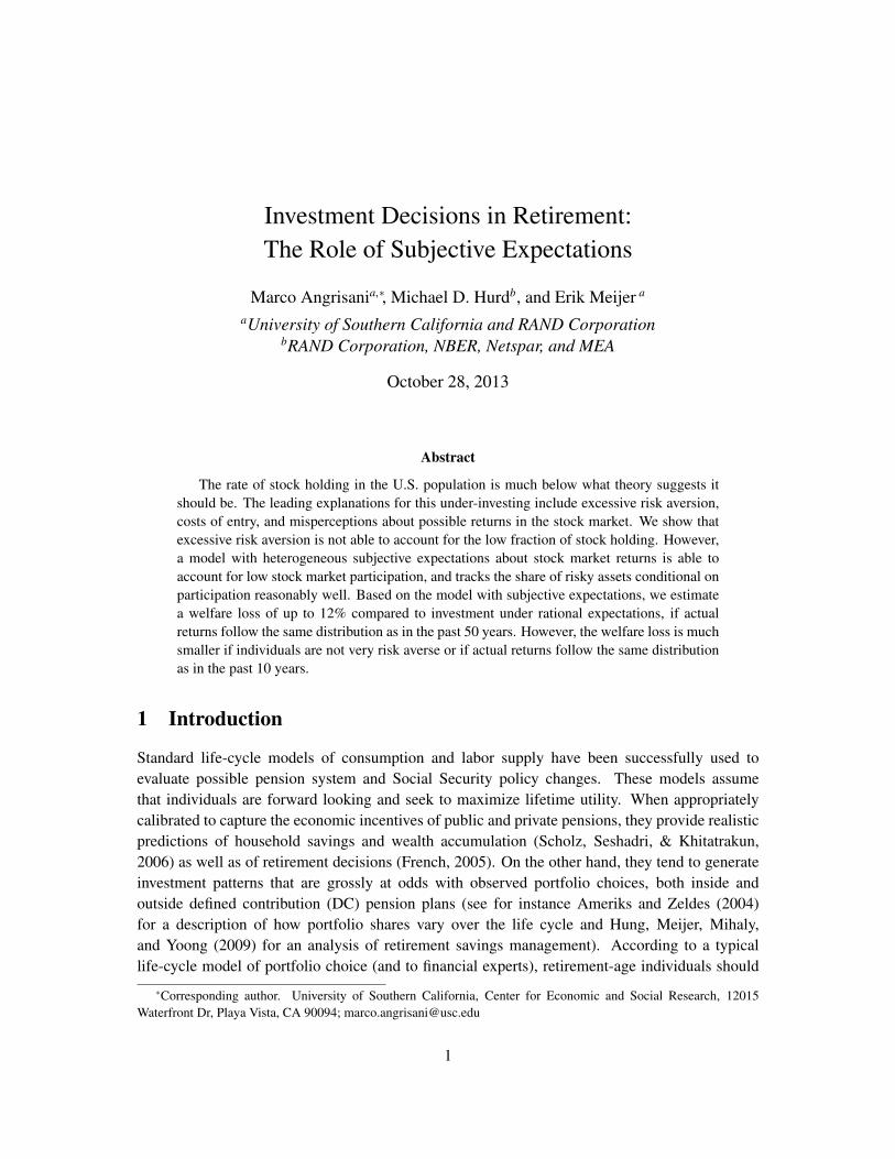
We consider stocks as the risky asset. Figure 1 shows the fraction of individuals in our samplewho hold stocks, and among those who hold stocks, what the average fraction of their wealthin stocks is. Stock holding is relatively constant across age at slightly below 40%, whereas theshare of risky assets slopes upward a little with increasing age.3 In the following sections, we willpresent analogous patterns based on the model’s predictions and compare them to their empiricalcounterparts.

Two auxiliary models inform the life-cycle model presented above. The first is used to estimateconditional survival and health transition probabilities. Following De Nardi et al. (2010), we takethe unconditional survival probabilities from life tables and estimate the probabilities of beingin a given health status conditional on being currently alive, alive next year, in good and badhealth last year, from the data. These four conditional probabilities are specified as a functionof a cubic polynomial in age and jointly estimated by maximum likelihood. Observed two-yeartransitions are written as functions of these four conditional probabilities and life tables survivalprobabilities and inferred accordingly. One-year survival and transition probabilities are thenderived and used as inputs in the dynamic programming problem. The second auxiliary modeldeals with the process of out-of-pocket medical expenses. Equation (3) is expressed in terms ofmedical costs normalized to retirement income and estimated as a panel data regression modelwith individual and year fixed effects, a cubic polynomial in age, and an interaction of healthand age. The specification and estimation of the auxiliary models is discussed in more details inAppendix C.

The remaining parameters of the model—tax rates, the inflation rate, the distribution of assetreturns, the discount factor, and relative risk aversion—are taken from the literature or externaldata sources. Table 1 summarizes the values for the baseline model’s parameters. See Appendix Dfor further details.

3Several reasons may explain the observed increase in the share of risky assets at very old ages. For example,retirees may spend down their non-equity wealth before tapping their stock market investments. Also, mortality mayplay a role, as richer and more educated individuals are more likely to hold stocks and live longer.

7

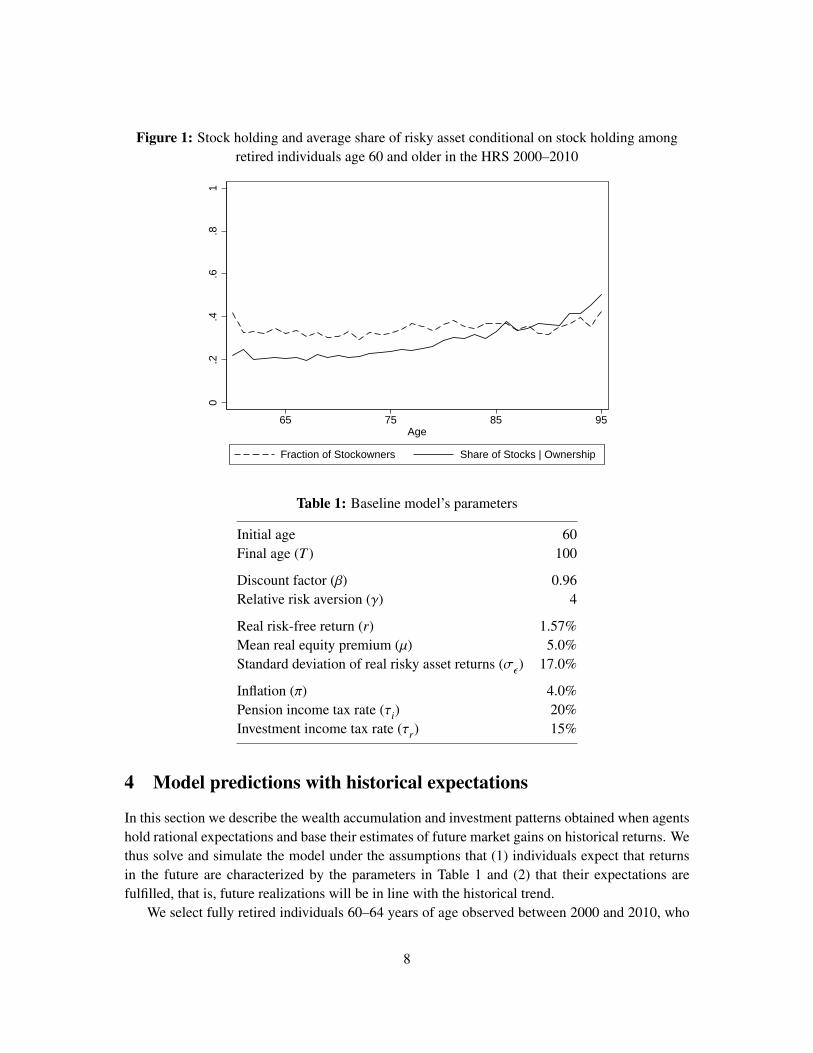
Figure 1: Stock holding and average share of risky asset conditional on stock holding amongretired individuals age 60 and older in the HRS 2000–2010

0.2

.4.6

.81

65 75 85 95Age

Fraction of Stockowners Share of Stocks | Ownership

®

Table 1: Baseline model’s parameters

Initial age 60Final age (T ) 100

Discount factor (β) 0.96Relative risk aversion (γ) 4

Real risk-free return (r) 1.57%Mean real equity premium (µ) 5.0%Standard deviation of real risky asset returns (σε) 17.0%

Inflation (π) 4.0%Pension income tax rate (τi) 20%Investment income tax rate (τr) 15%

4 Model predictions with historical expectations

In this section we describe the wealth accumulation and investment patterns obtained when agentshold rational expectations and base their estimates of future market gains on historical returns. Wethus solve and simulate the model under the assumptions that (1) individuals expect that returnsin the future are characterized by the parameters in Table 1 and (2) that their expectations arefulfilled, that is, future realizations will be in line with the historical trend.

We select fully retired individuals 60–64 years of age observed between 2000 and 2010, who

8

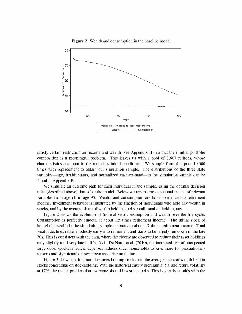
Figure 2: Wealth and consumption in the baseline model

05

1015

20N

orm

aliz

ed V

aria

bles

65 75 85 95Age

Wealth Consumption

Variables Normalized to Retirement Income

®

satisfy certain restriction on income and wealth (see Appendix B), so that their initial portfoliocomposition is a meaningful problem. This leaves us with a pool of 3,607 retirees, whosecharacteristics are input in the model as initial conditions. We sample from this pool 10,000times with replacement to obtain our simulation sample. The distributions of the three statevariables—age, health status, and normalized cash-on-hand—in the simulation sample can befound in Appendix B.

We simulate an outcome path for each individual in the sample, using the optimal decisionrules (described above) that solve the model. Below we report cross-sectional means of relevantvariables from age 60 to age 95. Wealth and consumption are both normalized to retirementincome. Investment behavior is illustrated by the fraction of individuals who hold any wealth instocks, and by the average share of wealth held in stocks conditional on holding any.

Figure 2 shows the evolution of (normalized) consumption and wealth over the life cycle.Consumption is perfectly smooth at about 1.5 times retirement income. The initial stock ofhousehold wealth in the simulation sample amounts to about 17 times retirement income. Totalwealth declines rather modestly early into retirement and starts to be largely run down in the late70s. This is consistent with the data, where the elderly are observed to reduce their asset holdingsonly slightly until very late in life. As in De Nardi et al. (2010), the increased risk of unexpectedlarge out-of-pocket medical expenses induces older households to save more for precautionaryreasons and significantly slows down asset decumulation.

Figure 3 shows the fraction of retirees holding stocks and the average share of wealth held instocks conditional on stockholding. With the historical equity premium at 5% and return volatilityat 17%, the model predicts that everyone should invest in stocks. This is greatly at odds with the

9

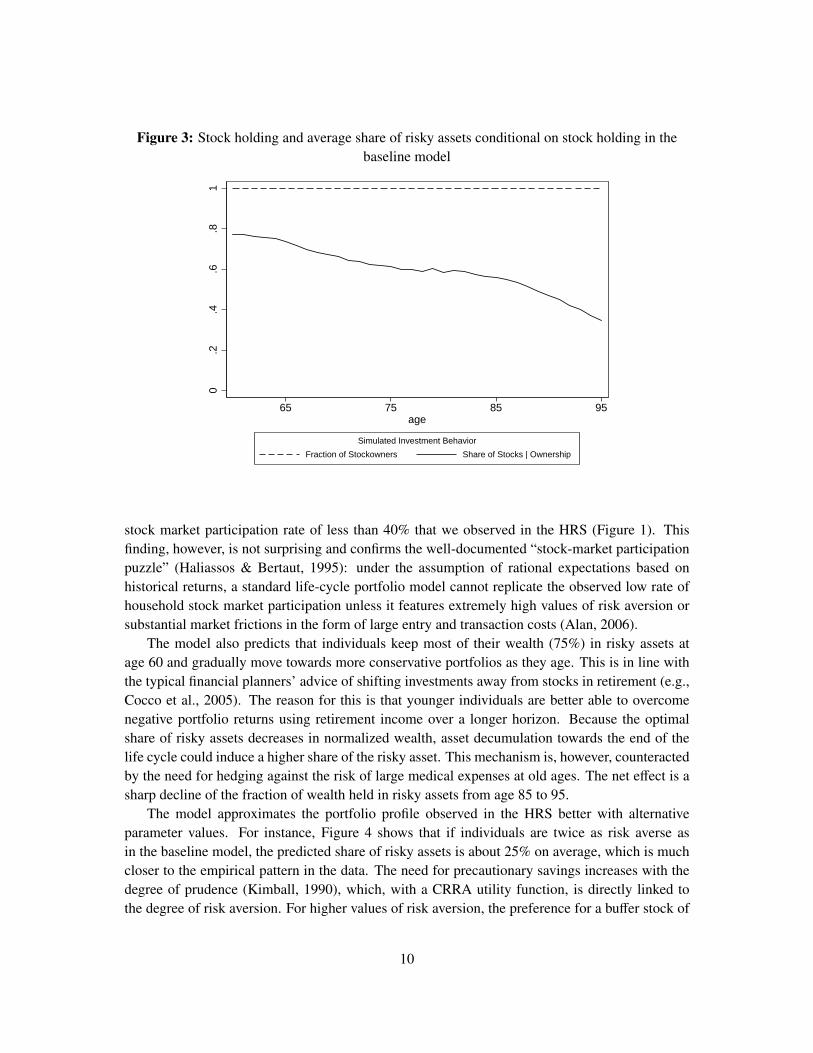
Figure 3: Stock holding and average share of risky assets conditional on stock holding in thebaseline model

0.2

.4.6

.81

65 75 85 95age

Fraction of Stockowners Share of Stocks | Ownership

Simulated Investment Behavior

®

stock market participation rate of less than 40% that we observed in the HRS (Figure 1). Thisfinding, however, is not surprising and confirms the well-documented “stock-market participationpuzzle” (Haliassos & Bertaut, 1995): under the assumption of rational expectations based onhistorical returns, a standard life-cycle portfolio model cannot replicate the observed low rate ofhousehold stock market participation unless it features extremely high values of risk aversion orsubstantial market frictions in the form of large entry and transaction costs (Alan, 2006).

The model also predicts that individuals keep most of their wealth (75%) in risky assets atage 60 and gradually move towards more conservative portfolios as they age. This is in line withthe typical financial planners’ advice of shifting investments away from stocks in retirement (e.g.,Cocco et al., 2005). The reason for this is that younger individuals are better able to overcomenegative portfolio returns using retirement income over a longer horizon. Because the optimalshare of risky assets decreases in normalized wealth, asset decumulation towards the end of thelife cycle could induce a higher share of the risky asset. This mechanism is, however, counteractedby the need for hedging against the risk of large medical expenses at old ages. The net effect is asharp decline of the fraction of wealth held in risky assets from age 85 to 95.

The model approximates the portfolio profile observed in the HRS better with alternativeparameter values. For instance, Figure 4 shows that if individuals are twice as risk averse asin the baseline model, the predicted share of risky assets is about 25% on average, which is muchcloser to the empirical pattern in the data. The need for precautionary savings increases with thedegree of prudence (Kimball, 1990), which, with a CRRA utility function, is directly linked tothe degree of risk aversion. For higher values of risk aversion, the preference for a buffer stock of

10

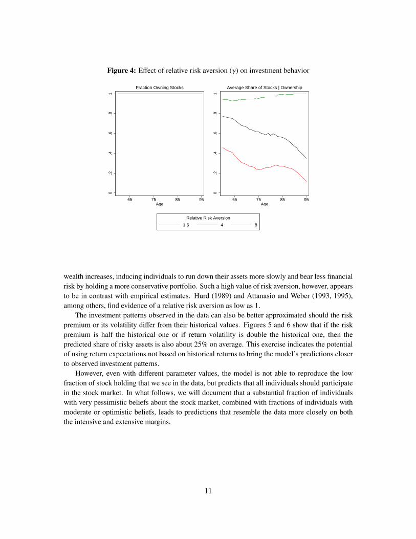
Figure 4: Effect of relative risk aversion (γ) on investment behavior

0.2

.4.6

.81

65 75 85 95Age

Fraction Owning Stocks

0.2

.4.6

.81

65 75 85 95Age

Average Share of Stocks | Ownership

1.5 4 8

Relative Risk Aversion

®

wealth increases, inducing individuals to run down their assets more slowly and bear less financialrisk by holding a more conservative portfolio. Such a high value of risk aversion, however, appearsto be in contrast with empirical estimates. Hurd (1989) and Attanasio and Weber (1993, 1995),among others, find evidence of a relative risk aversion as low as 1.

The investment patterns observed in the data can also be better approximated should the riskpremium or its volatility differ from their historical values. Figures 5 and 6 show that if the riskpremium is half the historical one or if return volatility is double the historical one, then thepredicted share of risky assets is also about 25% on average. This exercise indicates the potentialof using return expectations not based on historical returns to bring the model’s predictions closerto observed investment patterns.

However, even with different parameter values, the model is not able to reproduce the lowfraction of stock holding that we see in the data, but predicts that all individuals should participatein the stock market. In what follows, we will document that a substantial fraction of individualswith very pessimistic beliefs about the stock market, combined with fractions of individuals withmoderate or optimistic beliefs, leads to predictions that resemble the data more closely on boththe intensive and extensive margins.

11

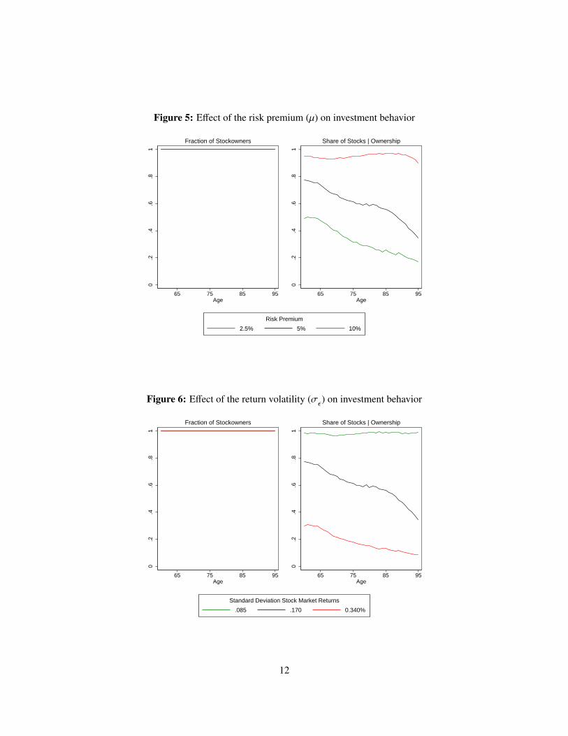
Figure 5: Effect of the risk premium (µ) on investment behavior

0.2

.4.6

.81

65 75 85 95Age

Fraction of Stockowners

0.2

.4.6

.81

65 75 85 95Age

Share of Stocks | Ownership

2.5% 5% 10%

Risk Premium

®

Figure 6: Effect of the return volatility (σε) on investment behavior

0.2

.4.6

.81

65 75 85 95Age

Fraction of Stockowners

0.2

.4.6

.81

65 75 85 95Age

Share of Stocks | Ownership

.085 .170 0.340%

Standard Deviation Stock Market Returns

®

12

5 Subjective beliefs about the distribution of stock market returns

Since 2002, the HRS has elicited respondents’ beliefs about stock market returns. The basicquestion, asked in each wave, is:

By next year at this time, what is the percent chance that mutual fund shares investedin blue chip stocks like those in the Dow Jones Industrial Average will be worth morethan they are today?

We call this question P0. From 2006 onward, a follow-up question has been added to understandwhether a 50% answer to P0 expresses epistemic uncertainty. In 2008, follow-up questions havebeen introduced after 0% and 100% answers to P0 so as to gain insight on whether these arerounded (in which case respondents are probed again to give a continuous answer) or actual beliefsof certainty. We take all this information into account when using answers to P0.

In 2002, one additional question, which we call P10, similarly asked the percent chance thatthey have grown by 10 percent or more, with the order of P0 and P10 randomized between twogroups.

In 2010, two similar questions were asked. P20 asks about 20 percent gain and P[−20] asksthe percent chance that stocks will fall by more than 20 percent.

In 2008, respondents were randomized into one of 8 follow-up questions after answering P0and asked about the probability of stock market gains of 10, 20, 30, or 40 percent (P10 – P40)or losses of 10, 20, 30, or 40 percent (P[−10] – P[−40]). Each respondent answered at most twoquestions, P0 and one follow-up.

Summarizing, for the distribution of the one-year ahead stock market return, HRS respondentsgave one probability in 2004 and 2006, up to two probabilities in 2002 and 2008, and up to threeprobabilities in 2010. Under suitable assumptions, we can use these self-reported probabilitiesto compute individual-specific distributions of stock market returns. Throughout, we assume thatthese questions elicit beliefs about nominal before-tax returns.

Dominitz and Manski (2007) study the 2004 data, which only have P0. They assume thatrespondents’ subjective distributions of stock market returns are normal with a constant standarddeviation equal to the historical standard deviation of nominal returns (for which they use 0.206).Under these assumptions, the 2004 data can be exploited to infer individual-specific expected stockmarket returns. Let mi be respondent i’s subjective mean, si = s, ∀i, be respondent i’s subjectivestandard deviation, and p0i be the answer to P0 divided by 100. Then mi = −sΦ−1(1 − p0i),where Φ(·) is the standard normal cumulative distribution function. This method can be used forthe 2004 and 2006 data. This method can be generalized if more information is available. Forinstance, whenever respondents give two probabilistic answers, the assumption that si is constantacross individuals can be relaxed and both the subjective mean and standard deviation of thedistributions of returns can be inferred. Specifically, denoting with pxi and pyi the probabilitiesof a stock market gain of at least x and y, respectively (e.g., x = 0 and y = 0.10 in 2002), the

13

following system of two equations in two unknowns can be solved:

si =y − x

Φ−1(1 − pyi) − Φ−1(1 − pxi)(10a)

mi = x − siΦ−1(1 − pxi) =

x Φ−1(1 − pyi) − y Φ−1(1 − pxi)

Φ−1(1 − pyi) − Φ−1(1 − pxi). (10b)

When, as in 2010, three probabilistic questions are asked, the two parameters mi and si would beover-identified (a system of three equations in two unknowns). In this case a minimum distanceestimation procedure could be applied to obtain subjective means and standard deviations ofindividual-specific return distributions.

Hurd and Rohwedder (2011) take a different approach. They observe that respondents’answers to k questions reveal subjective probabilities that stock market returns take values withink + 1 mutually exclusive intervals spanning the entire real line. They proceed to assume thatthe subjective distribution within each interval coincides with the historical distribution withinthat interval. For example, suppose the respondent answers only P0. From this we can deducePri(r

e < 0) and Pri(re ≥ 0), where re is the nominal stock market return (as in the model of

section 2) and the subscript i denotes respondent i’s subjective distribution. Then

Ei(re) = Pri(r

e < 0)E(re | re < 0) + Pri(re ≥ 0)E(re | re ≥ 0)

Ei[(re)2] = Pri(r

e < 0)E[(re)2 | re < 0

]+ Pri(r

e ≥ 0)E[(re)2 | re ≥ 0

].

The conditional expectations on the right-hand side are taken from historical distributions, and thesubjective mean and standard deviations are obtained as mi = Ei(r

e) and si ={Ei

[(re)2] − m2

i

}1/2.

This method immediately generalizes to any number of intervals.We have experimented with both approaches and found that they give very similar results.

Here, we only present results using the Hurd-Rohwedder approach.4

After computing subjective means and standard deviations of nominal returns, we transformthem by correcting for inflation and the risk-free return so as to obtain the subjective real riskpremium and subjective standard deviation of real excess returns. For consistency with thesubjective expectations about stock returns, we should also use subjective expectations aboutinflation and the risk-free return. The HRS does not elicit subjective expectations about pricesand the risk-free interest rate, but the Survey of Consumers (http://www.sca.isr.umich.edu/)does. The average subjective inflation rate reported by individuals in the Survey of Consumers

4We use basic probability rules to identify inconsistent answers. First, we drop self-reported probabilities that areoutside the [0, 1] interval. The procedure suggested by Dominitz and Manski (2007) implies that only values strictlygreater than 0 and strictly less than 1 can be used. Given that a significant fraction of the respondents clusters at 0 or 1,we approximate a “zero probability” with 0.001 and a “one probability” with 0.999. This allows us to retain most of theselected individuals in the sample when estimating subjective distributions of returns. The Hurd-Rohwedder approachdoes not require this approximation as it can be implemented for probabilities taking value 0 or 1. Second, when two ormore probabilities are elicited, we define as inconsistent all answers that do not conform to the probabilities of the singleevents and their union. If, for instance P0 and P10 are asked, we define as inconsistent all answers for which P0 ≤ P10.In this case, we only use P0 and ignore P10. The inequality above is required to be strict under the Dominitz-Manskiapproach, but not under the Hurd-Rohwedder approach.

14

over the period 2002–2010 is 3.75%. We use this value to compute the subjective real expectedstock market returns from the subjective nominal stock market returns. The Survey of Consumersasks its respondents if they expect any change in interest rates during the next 12 months, butnot what the expected interest rate will be. However, most respondents expect the interest rate inthe coming year to be about the same as the interest rate in the past year. Therefore, in order toconstruct a proxy of the subjective real interest rate, we take the average nominal interest rate from2002 to 2010 and correct it by the aforementioned expected inflation rate of 3.75%. This returns areal interest rate of 0.3%, which we use in the computation.

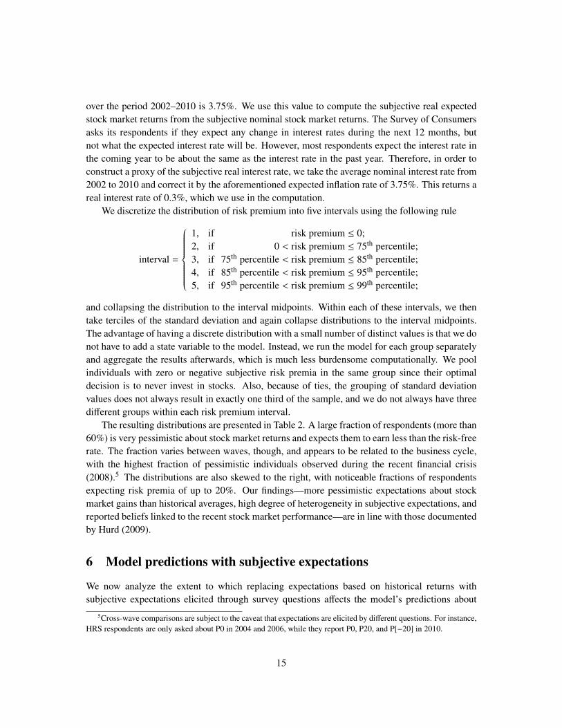
We discretize the distribution of risk premium into five intervals using the following rule

interval =

1, if risk premium ≤ 0;2, if 0 < risk premium ≤ 75th percentile;3, if 75th percentile < risk premium ≤ 85th percentile;4, if 85th percentile < risk premium ≤ 95th percentile;5, if 95th percentile < risk premium ≤ 99th percentile;

and collapsing the distribution to the interval midpoints. Within each of these intervals, we thentake terciles of the standard deviation and again collapse distributions to the interval midpoints.The advantage of having a discrete distribution with a small number of distinct values is that we donot have to add a state variable to the model. Instead, we run the model for each group separatelyand aggregate the results afterwards, which is much less burdensome computationally. We poolindividuals with zero or negative subjective risk premia in the same group since their optimaldecision is to never invest in stocks. Also, because of ties, the grouping of standard deviationvalues does not always result in exactly one third of the sample, and we do not always have threedifferent groups within each risk premium interval.

The resulting distributions are presented in Table 2. A large fraction of respondents (more than60%) is very pessimistic about stock market returns and expects them to earn less than the risk-freerate. The fraction varies between waves, though, and appears to be related to the business cycle,with the highest fraction of pessimistic individuals observed during the recent financial crisis(2008).5 The distributions are also skewed to the right, with noticeable fractions of respondentsexpecting risk premia of up to 20%. Our findings—more pessimistic expectations about stockmarket gains than historical averages, high degree of heterogeneity in subjective expectations, andreported beliefs linked to the recent stock market performance—are in line with those documentedby Hurd (2009).

6 Model predictions with subjective expectations

We now analyze the extent to which replacing expectations based on historical returns withsubjective expectations elicited through survey questions affects the model’s predictions about

5Cross-wave comparisons are subject to the caveat that expectations are elicited by different questions. For instance,HRS respondents are only asked about P0 in 2004 and 2006, while they report P0, P20, and P[−20] in 2010.

15

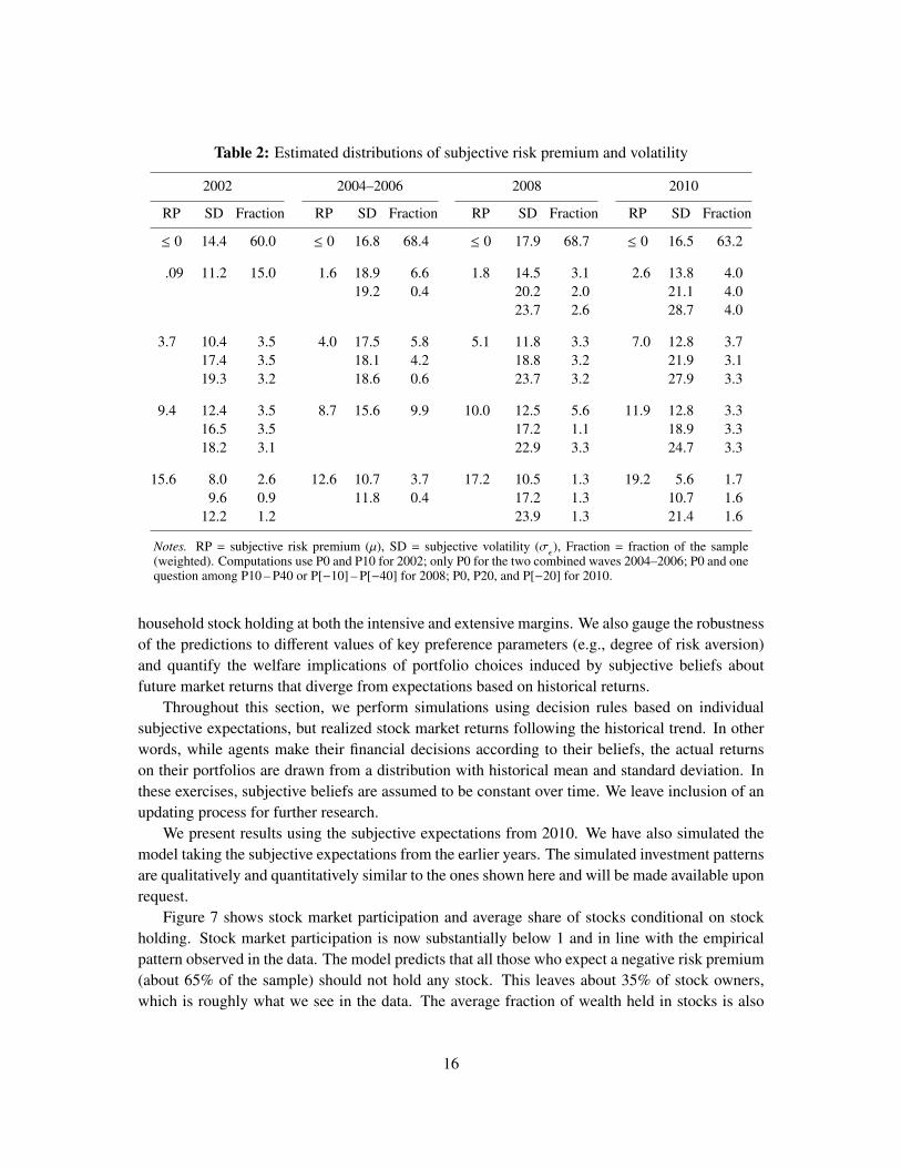
Table 2: Estimated distributions of subjective risk premium and volatility

2002 2004–2006 2008 2010

RP SD Fraction RP SD Fraction RP SD Fraction RP SD Fraction

≤ 0 14.4 60.0 ≤ 0 16.8 68.4 ≤ 0 17.9 68.7 ≤ 0 16.5 63.2

.09 11.2 15.0 1.6 18.9 6.6 1.8 14.5 3.1 2.6 13.8 4.019.2 0.4 20.2 2.0 21.1 4.0

23.7 2.6 28.7 4.0

3.7 10.4 3.5 4.0 17.5 5.8 5.1 11.8 3.3 7.0 12.8 3.717.4 3.5 18.1 4.2 18.8 3.2 21.9 3.119.3 3.2 18.6 0.6 23.7 3.2 27.9 3.3

9.4 12.4 3.5 8.7 15.6 9.9 10.0 12.5 5.6 11.9 12.8 3.316.5 3.5 17.2 1.1 18.9 3.318.2 3.1 22.9 3.3 24.7 3.3

15.6 8.0 2.6 12.6 10.7 3.7 17.2 10.5 1.3 19.2 5.6 1.79.6 0.9 11.8 0.4 17.2 1.3 10.7 1.6

12.2 1.2 23.9 1.3 21.4 1.6

Notes. RP = subjective risk premium (µ), SD = subjective volatility (σε), Fraction = fraction of the sample

(weighted). Computations use P0 and P10 for 2002; only P0 for the two combined waves 2004–2006; P0 and onequestion among P10 – P40 or P[−10] – P[−40] for 2008; P0, P20, and P[−20] for 2010.

household stock holding at both the intensive and extensive margins. We also gauge the robustnessof the predictions to different values of key preference parameters (e.g., degree of risk aversion)and quantify the welfare implications of portfolio choices induced by subjective beliefs aboutfuture market returns that diverge from expectations based on historical returns.

Throughout this section, we perform simulations using decision rules based on individualsubjective expectations, but realized stock market returns following the historical trend. In otherwords, while agents make their financial decisions according to their beliefs, the actual returnson their portfolios are drawn from a distribution with historical mean and standard deviation. Inthese exercises, subjective beliefs are assumed to be constant over time. We leave inclusion of anupdating process for further research.

We present results using the subjective expectations from 2010. We have also simulated themodel taking the subjective expectations from the earlier years. The simulated investment patternsare qualitatively and quantitatively similar to the ones shown here and will be made available uponrequest.

Figure 7 shows stock market participation and average share of stocks conditional on stockholding. Stock market participation is now substantially below 1 and in line with the empiricalpattern observed in the data. The model predicts that all those who expect a negative risk premium(about 65% of the sample) should not hold any stock. This leaves about 35% of stock owners,which is roughly what we see in the data. The average fraction of wealth held in stocks is also

16

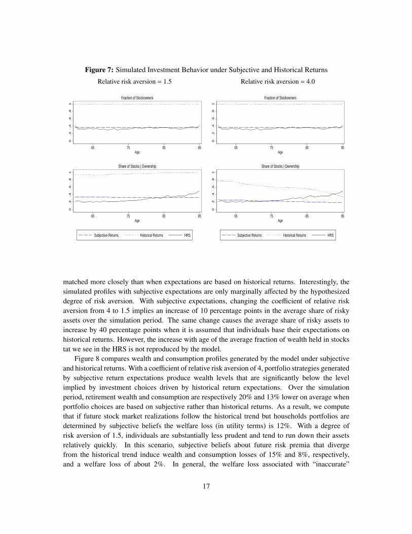
Figure 7: Simulated Investment Behavior under Subjective and Historical Returns

Relative risk aversion = 1.5 Relative risk aversion = 4.0

0.2

.4.6

.81

65 75 85 95Age

Fraction of Stockowners

0.2

.4.6

.81

65 75 85 95Age

Share of Stocks | Ownership

Subjective Returns Historical Returns HRS

®

0.2

.4.6

.81

65 75 85 95Age

Fraction of Stockowners

0.2

.4.6

.81

65 75 85 95Age

Share of Stocks | Ownership

Subjective Returns Historical Returns HRS

®

matched more closely than when expectations are based on historical returns. Interestingly, thesimulated profiles with subjective expectations are only marginally affected by the hypothesizeddegree of risk aversion. With subjective expectations, changing the coefficient of relative riskaversion from 4 to 1.5 implies an increase of 10 percentage points in the average share of riskyassets over the simulation period. The same change causes the average share of risky assets toincrease by 40 percentage points when it is assumed that individuals base their expectations onhistorical returns. However, the increase with age of the average fraction of wealth held in stockstat we see in the HRS is not reproduced by the model.

Figure 8 compares wealth and consumption profiles generated by the model under subjectiveand historical returns. With a coefficient of relative risk aversion of 4, portfolio strategies generatedby subjective return expectations produce wealth levels that are significantly below the levelimplied by investment choices driven by historical return expectations. Over the simulationperiod, retirement wealth and consumption are respectively 20% and 13% lower on average whenportfolio choices are based on subjective rather than historical returns. As a result, we computethat if future stock market realizations follow the historical trend but households portfolios aredetermined by subjective beliefs the welfare loss (in utility terms) is 12%. With a degree ofrisk aversion of 1.5, individuals are substantially less prudent and tend to run down their assetsrelatively quickly. In this scenario, subjective beliefs about future risk premia that divergefrom the historical trend induce wealth and consumption losses of 15% and 8%, respectively,and a welfare loss of about 2%. In general, the welfare loss associated with “inaccurate”

17

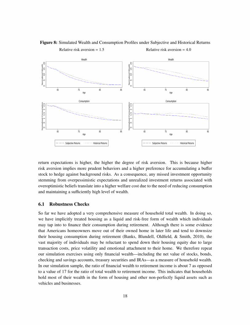
Figure 8: Simulated Wealth and Consumption Profiles under Subjective and Historical Returns

Relative risk aversion = 1.5 Relative risk aversion = 4.0

05

10

15

20

Norm

alized W

ealth

65 75 85 95Age

Wealth

0.5

11.5

22.5

Norm

alized C

onsum

ption

65 75 85 95Age

Consumption

Subjective Returns Historical Returns

®

05

10

15

20

Norm

alized W

ealth

65 75 85 95Age

Wealth

0.5

11.5

22.5

Norm

alized C

onsum

ption

65 75 85 95Age

Consumption

Subjective Returns Historical Returns

®

return expectations is higher, the higher the degree of risk aversion. This is because higherrisk aversion implies more prudent behaviors and a higher preference for accumulating a bufferstock to hedge against background risks. As a consequence, any missed investment opportunitystemming from overpessimistic expectations and unrealized investment returns associated withoveroptimistic beliefs translate into a higher welfare cost due to the need of reducing consumptionand maintaining a sufficiently high level of wealth.

6.1 Robustness Checks

So far we have adopted a very comprehensive measure of household total wealth. In doing so,we have implicitly treated housing as a liquid and risk-free form of wealth which individualsmay tap into to finance their consumption during retirement. Although there is some evidencethat Americans homeowners move out of their owned home in later life and tend to downsizetheir housing consumption during retirement (Banks, Blundell, Oldfield, & Smith, 2010), thevast majority of individuals may be reluctant to spend down their housing equity due to largetransaction costs, price volatility and emotional attachment to their home. We therefore repeatour simulation exercises using only financial wealth—including the net value of stocks, bonds,checking and savings accounts, treasury securities and IRAs—as a measure of household wealth.In our simulation sample, the ratio of financial wealth to retirement income is about 7 as opposedto a value of 17 for the ratio of total wealth to retirement income. This indicates that householdshold most of their wealth in the form of housing and other non-perfectly liquid assets such asvehicles and businesses.

18

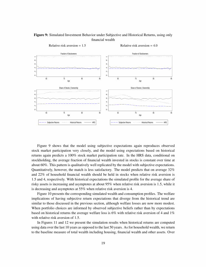
Figure 9: Simulated Investment Behavior under Subjective and Historical Returns, using onlyfinancial wealth

Relative risk aversion = 1.5 Relative risk aversion = 4.0

0.2

.4.6

.81

65 75 85 95Age

Fraction of Stockowners

0.2

.4.6

.81

65 75 85 95Age

Share of Stocks | Ownership

Subjective Returns Historical Returns HRS

®

0.2

.4.6

.81

65 75 85 95Age

Fraction of Stockowners

0.2

.4.6

.81

65 75 85 95Age

Share of Stocks | Ownership

Subjective Returns Historical Returns HRS

®

Figure 9 shows that the model using subjective expectations again reproduces observedstock market participation very closely, and the model using expectations based on historicalreturns again predicts a 100% stock market participation rate. In the HRS data, conditional onstockholding, the average fraction of financial wealth invested in stocks is constant over time atabout 60%. This pattern is qualitatively well replicated by the model with subjective expectations.Quantitatively, however, the match is less satisfactory. The model predicts that on average 32%and 22% of household financial wealth should be held in stocks when relative risk aversion is1.5 and 4, respectively. With historical expectations the simulated profile for the average share ofrisky assets is increasing and asymptotes at about 95% when relative risk aversion is 1.5, while itis decreasing and asymptotes at 55% when relative risk aversion is 4.

Figure 10 presents the corresponding simulated wealth and consumption profiles. The welfareimplications of having subjective return expectations that diverge from the historical trend aresimilar to those discussed in the previous section, although welfare losses are now more modest.When portfolio choices are informed by observed subjective beliefs rather than by expectationsbased on historical returns the average welfare loss is 6% with relative risk aversion of 4 and 1%with relative risk aversion of 1.5.

In Figures 11 and 12 we present the simulation results when historical returns are computedusing data over the last 10 years as opposed to the last 50 years. As for household wealth, we returnto the baseline measure of total wealth including housing, financial wealth and other assets. Over

19

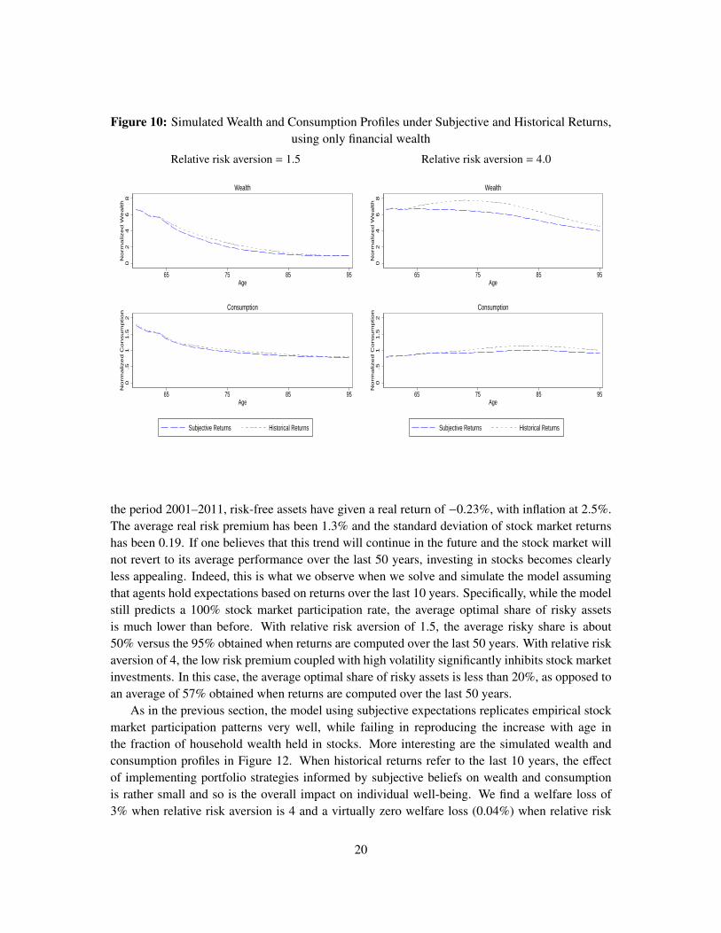
Figure 10: Simulated Wealth and Consumption Profiles under Subjective and Historical Returns,using only financial wealth

Relative risk aversion = 1.5 Relative risk aversion = 4.0

02

46

8N

orm

alized W

ealth

65 75 85 95Age

Wealth

0.5

11.5

2N

orm

alized C

onsum

ption

65 75 85 95Age

Consumption

Subjective Returns Historical Returns

®

02

46

8N

orm

alized W

ealth

65 75 85 95Age

Wealth

0.5

11.5

2N

orm

alized C

onsum

ption

65 75 85 95Age

Consumption

Subjective Returns Historical Returns

®

the period 2001–2011, risk-free assets have given a real return of −0.23%, with inflation at 2.5%.The average real risk premium has been 1.3% and the standard deviation of stock market returnshas been 0.19. If one believes that this trend will continue in the future and the stock market willnot revert to its average performance over the last 50 years, investing in stocks becomes clearlyless appealing. Indeed, this is what we observe when we solve and simulate the model assumingthat agents hold expectations based on returns over the last 10 years. Specifically, while the modelstill predicts a 100% stock market participation rate, the average optimal share of risky assetsis much lower than before. With relative risk aversion of 1.5, the average risky share is about50% versus the 95% obtained when returns are computed over the last 50 years. With relative riskaversion of 4, the low risk premium coupled with high volatility significantly inhibits stock marketinvestments. In this case, the average optimal share of risky assets is less than 20%, as opposed toan average of 57% obtained when returns are computed over the last 50 years.

As in the previous section, the model using subjective expectations replicates empirical stockmarket participation patterns very well, while failing in reproducing the increase with age inthe fraction of household wealth held in stocks. More interesting are the simulated wealth andconsumption profiles in Figure 12. When historical returns refer to the last 10 years, the effectof implementing portfolio strategies informed by subjective beliefs on wealth and consumptionis rather small and so is the overall impact on individual well-being. We find a welfare loss of3% when relative risk aversion is 4 and a virtually zero welfare loss (0.04%) when relative risk

20

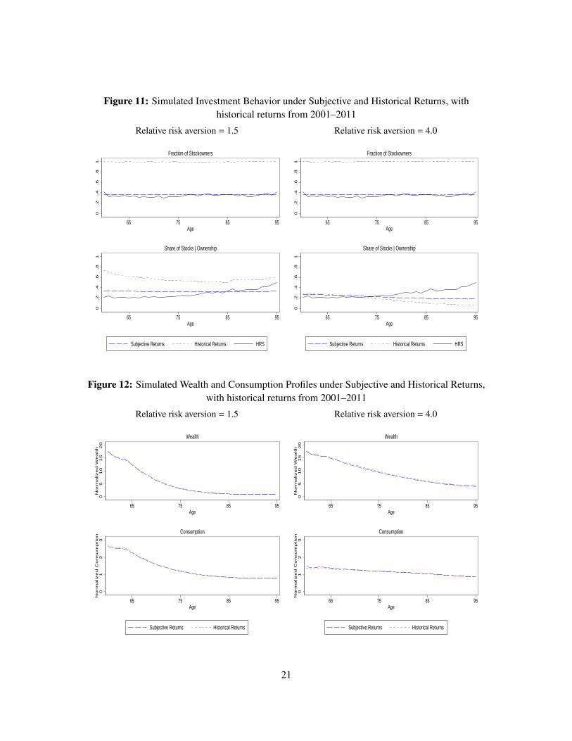
Figure 11: Simulated Investment Behavior under Subjective and Historical Returns, withhistorical returns from 2001–2011

Relative risk aversion = 1.5 Relative risk aversion = 4.0

0.2

.4.6

.81

65 75 85 95Age

Fraction of Stockowners

0.2

.4.6

.81

65 75 85 95Age

Share of Stocks | Ownership

Subjective Returns Historical Returns HRS

®

0.2

.4.6

.81

65 75 85 95Age

Fraction of Stockowners

0.2

.4.6

.81

65 75 85 95Age

Share of Stocks | Ownership

Subjective Returns Historical Returns HRS

®

Figure 12: Simulated Wealth and Consumption Profiles under Subjective and Historical Returns,with historical returns from 2001–2011

Relative risk aversion = 1.5 Relative risk aversion = 4.0

05

10

15

20

Norm

alized W

ealth

65 75 85 95Age

Wealth

01

23

Norm

alized C

onsum

ption

65 75 85 95Age

Consumption

Subjective Returns Historical Returns

®

05

10

15

20

Norm

alized W

ealth

65 75 85 95Age

Wealth

01

23

Norm

alized C

onsum

ption

65 75 85 95Age

Consumption

Subjective Returns Historical Returns

®

21

aversion is 1.5.

7 Discussion

Standard life cycle models of economic behavior predict that essentially everybody should investin risky assets to some extent, which is greatly at odds with the less than 40% of households that areobserved to own stocks in the data. Moreover, conditional on stock holding, standard models withrealistic values of preference parameters predict much higher fractions of wealth invested in riskyassets than we observe in the data. Several explanations have been put forward in the literature,but none has been able to fully reconcile theoretical predictions with observed empirical patterns.

In this paper, we explore to what extent subjective expectations about stock market returnsthat differ from historical returns can address the so-called “stock-market participation puzzle”.We embed subjective expectations in an otherwise relatively standard economic life cycle model.Using data on subjective expectations from the Health and Retirement Study, we show that a largefraction of the population holds beliefs that are so pessimistic that they should never invest instocks. Of the remaining individuals, a nonnegligible fraction is very optimistic and they shouldinvest almost all of their wealth in risky assets. A “moderate” middle group rounds out thedistribution and is predicted to keep some but not all of its wealth in risky assets. The modelwith these heterogeneous subjective expectations is remarkably well able to match the empiricalpatterns in household stock market participation. The matching of observed portfolio shares is lesssatisfactory. In particular, while the model predicts that portfolio shares should gradually decreaseover time, the fraction of wealth invested in stocks slightly increases with age in the data. Mostlikely this is a selection effect due to running down different asset categories, stock holding, andmortality being correlated.

Our model simulations also show that when subjective beliefs diverge from historical returns,portfolio choices informed by the former have important welfare consequences. We estimatewelfare losses ranging between 2% and 12%, depending on the degree of individual risk aversionand the way historical returns are computed. We also find that welfare losses are larger, the higherthe degree of risk aversion.

The current model assumes that different individuals may have different expectations, but theykeep the same expectations throughout their lifetimes. In practice, optimistic individuals whoconsume much and expect the asset returns to support their life style may notice a systematicrundown of their assets caused by lower returns than expected. They may respond to this byupdating their expectations and behaving more cautiously in later life. Moreover, we have seen thatin the data, subjective expectations vary between waves and may be related to the business cycle.This suggests a role for the business cycle in changing expectations as well. Therefore, extendingthe model with a mechanism for updating beliefs is an important topic for future research.

Our model contains risks of medical expenses as estimated from the HRS data. If individualshold beliefs about their likelihood of being in good health or about the risks of large medicalexpenses conditional on health status that are different from historical distributions, these mayalso impact individuals’ behavior. We have performed limited experiments with subjective

22

distributions of health transitions, but these did not have much effect on the results. However,it is worthwhile to study this more systematically and focus on expectations about out-of-pocketmedical expenses directly.

Acknowledgments

This study was funded by the Social Security Administration through the University of MichiganRetirement Research Center (MRRC), grant number UM12-13. We would like to thank seminarparticipants at Erasmus University Rotterdam, VU University Amsterdam, the 2012 MRRCResearcher Workshop, the IMT Institute for Advanced Studies Lucca, and the All California LaborConference 2012 for helpful comments and stimulating discussions.

Appendix

A Model’s Solution

Normalization Consider the model set-up of section 2 and let lowercase letters indicate theratios of the original variables to the level of retirement income (e.g., xt = Xt/P). Then expectedremaining lifetime utility (8) is

Ut = P1−γ

c1−γt

1 − γ+ Et

TM∑

j=t+1

β j−tc1−γ

j

1 − γ

, (A.1)

where TM is stochastic length of life.Using the definition of cash on hand Xt in the text, the wealth transition (7) can be rewritten as

xt+1 =[αt(1 + re

t+1) + (1 − αt)(1 + r)]

(xt − ct) + (1 − τi) − hct+1. (A.2)

Clearly, P does not play any role in the utility function and it is eliminated from the wealthtransition equation. Thus, exploiting the scale-independence of the original maximizationproblem, we can rewrite all variables as ratios to the constant flow of retirement income and reducethe dimensionality of the problem from 4 state variables—cash-on-hand, retirement income, age,and health status—to 3 state variables—normalized cash-on-hand, age, and health status. Thisrenormalization, introduced by Carroll (1992, 1997), makes the numerical problem more tractableas it significantly decreases the computational burden. Carroll (1992, 1997) shows that thisnormalization can also be applied to models featuring variable and uncertain income. Gomeset al. (2009) solve a model of saving and portfolio choice with taxable and tax-deferred accountsnormalizing all variables with respect to the permanent component of stochastic income.

After the normalization, the individual’s maximization problem can be expressed in recursiveform as follows:

vt(xt,Ht, t) = maxct ,αt

c1−γt

1 − γ+ βEt

[vt+1(xt+1,Ht+1, t + 1)

] , (A.3)

23

subject to (A.2) and wt ≥ 0, ∀t.Note that both xt+1 and Ht+1 are stochastic functions of {xt,Ht, ct, αt, t}, and the survival

probability is also part of the expectation.

Numerical solution The model is solved via backward induction, from the final period T = 100to the initial period t0 = 60. The state space is given by {xt,Ht, t}. In order to implementthis solution algorithm, we discretize the continuous state variable, normalized cash-on-hand, bydefining an equally spaced grid, {xk}

Kk=1. The upper bound is chosen to be nonbinding in all periods,

specifically xK = 99. The lower bound is set to 0.01. This can be interpreted as a minimum levelof consumption guaranteed by government transfers in all periods. By imposing xt ≥ 0.01 for allt, the model solution implicitly accounts for transfers from welfare programs equivalent to 1% ofretirement income plus medical expenses minus all available resources, if that amount is positive,and zero otherwise.

The optimization procedure combines a root-finding algorithm (Brent’s method; Brent, 1973,chapter 4) and standard grid search. For given values of xt and Ht, the value function is concavewith respect to ct. Thus, optimal normalized consumption can be computed using Brent’s method,significantly improving on computational efficiency. It is not known whether the value function isconcave in portfolio share αt. Hence, to avoid the potential danger of selecting local optima, weoptimize over the space of the remaining decision variable using a standard grid search. For thispurpose, we discretize the share of risky assets, α, to take 11 equally spaced values in the interval[0, 1].

Interpolation plays a crucial role in the solution of the dynamic programming problem athand. We use two-dimensional cubic splines interpolation to evaluate the value function betweenpoints on the cash-on-hand grid. Cubic splines have the advantage of being twice continuouslydifferentiable with a nonzero third derivative. These properties preserve the prudence of the utilityfunction, which plays an important role in precautionary savings and the effect of backgroundrisks on individual decisions (Eeckhoudt & Kimball, 1992; Kimball, 1990). The strictly positivelower bound on the grid for cash-on-hand implies that the value function is also bounded frombelow. This makes the spline interpolation work very well as long as the discretization of the statespace is sufficiently fine. Numerical integrations are performed by Gaussian quadrature.

B Data

Source and years We mainly use the RAND HRS (St.Clair et al., 2011), which is apostprocessed, more user-friendly version of the raw HRS data. We also add variables that arenot included in the main RAND HRS file, such as subjective expectations about stock marketreturns (which are in the RAND-enhanced FAT files) and detailed pension income data (from theRAND income and wealth imputations files). We use waves 5–10, which cover the period from2000 to 2010.

24

Unit of analysis The model as presented in section 2 is a model for the individual. In contrastwith this, information on wealth and asset allocation is at the household level in the HRS. Thus,in our estimation and simulation exercises, we use the household as our unit of analysis. Wealthand income are reported by the financial respondent, who is the one deemed most knowledgeableabout the household’s finances. Accordingly, for some inherently individual-level variables (age,mortality), we use the variables for the financial respondent.

Retirement income Household retirement income includes pension benefits, annuities, andSocial Security retirement received by the financial respondent and his or her spouse in eachwave. For each household, we first compute retirement income in each wave and then a constantflow of retirement income by averaging retirement income over all periods when it is observed.

Medical expenses Out-of-pocket medical expenses comprise the costs incurred in a year forhospital, nursing home, doctor visits, dentist, outpatient surgery, average monthly prescriptiondrug, home health care, and special facilities. Household out-of-pocket medical expenses areobtained summing the costs reported by the financial respondent and, if present, his or her spouse.

Health We define an individual to be in bad health if he or she reports his or her health status as“fair” or “poor”, and in good health otherwise. Because health costs are borne by the household,and economic decisions are made at the household level, the risk of health costs related to thespouse’s health must be taken into account. Therefore, in our analyses, we use an indicator of badhealth at the household level. The household is defined to be in bad health if either the respondentor the spouse (if any), or both are in bad health.

Assets The wealth measure for the baseline analysis includes net housing wealth (primary andsecondary residence, other real estate, minus balances of mortgages and other loans), vehicles,personal items of value, and net financial wealth (checking and savings accounts, certificates ofdeposit, bonds, stocks, businesses, IRAs, minus non-housing debt). In section 6.1, we presentrobustness checks that use only the financial assets component (without the amount of assets inbusinesses).

We consider stocks, held either directly or indirectly through an IRA, as the risky asset.We do not include balances in defined contribution (DC) pension plans in total wealth, nor thestock fraction of these balances in stock wealth, because these balances are not readily available.Gustman, Steinmeier, and Tabatabai (2010) construct measures of DC (and DB) pension wealthand the fraction of that invested in stocks, but the latter is only available for 2006, in which amongover 6,400 fully retired financial respondents 60 and over, less than 1% had stocks in a DC accountand therefore this omission does not influence our results.6

6The reasons for this are arguably that in this age group, relatively few individuals have DC plans and that uponretirement, many of those who do have a DC plan roll over their balances into an IRA or take out the pension in theform of a lump sum.

25

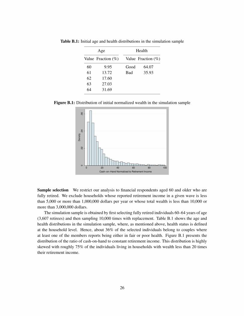
Table B.1: Initial age and health distributions in the simulation sample

Age Health

Value Fraction (%) Value Fraction (%)

60 9.95 Good 64.0761 13.72 Bad 35.9362 17.6063 27.0364 31.69

Figure B.1: Distribution of initial normalized wealth in the simulation sample

0.0

2.0

4.0

6D

en

sity

0 20 40 60 80 100

Cash−on−Hand Normalized to Retirement Income

Sample selection We restrict our analysis to financial respondents aged 60 and older who arefully retired. We exclude households whose reported retirement income in a given wave is lessthan 5,000 or more than 1,000,000 dollars per year or whose total wealth is less than 10,000 ormore than 3,000,000 dollars.

The simulation sample is obtained by first selecting fully retired individuals 60–64 years of age(3,607 retirees) and then sampling 10,000 times with replacement. Table B.1 shows the age andhealth distributions in the simulation sample, where, as mentioned above, health status is definedat the household level. Hence, about 36% of the selected individuals belong to couples whereat least one of the members reports being either in fair or poor health. Figure B.1 presents thedistribution of the ratio of cash-on-hand to constant retirement income. This distribution is highlyskewed with roughly 75% of the individuals living in households with wealth less than 20 timestheir retirement income.

26

C Auxiliary Models

C.1 Survival and health transition probabilities

The model has two interrelated transition processes: mortality and health transitions. We followDe Nardi et al. (2010) and others and assume that survival from age t−1 to age t, and health statusat age t conditional on survival, depend on health status at age t − 1. We cannot directly estimatethe one-year survival and health transition probabilities (1) – (2) from the HRS, because the HRSinterviews individuals every two years and thus we do not observe one-year transitions. This isonly a minor nuisance, because probabilities of two-year transitions follow from the probabilitiesof one-year transitions:

Φt(good | h) ≡ Pr(alivet,Ht = good | alivet−2,Ht−2 = h)

= sht−1

[φh

t−1sgoodt φ

goodt + (1 − φh

t−1)sbadt φbad

t

](C.1a)

Φt(bad | h) ≡ Pr(alivet,Ht = bad | alivet−2,Ht−2 = h)

= sht−1

[φh

t−1sgoodt (1 − φgood

t ) + (1 − φht−1)sbad

t (1 − φbadt )

](C.1b)

Φt(dead | h) ≡ Pr(deadt | alivet−2,Ht−2 = h)

= 1 − Φt(good | h) − Φt(bad | h). (C.1c)

The left-hand sides of these expressions are observable in the HRS and thus can be used to estimatethe one-year transition probabilities. However, the number of deaths in the HRS is insufficient toreliably estimate conditional survival rates directly. Therefore, as in De Nardi et al. (2010), wecombine information from the data with unconditional survival probabilities from life tables andBayes’ rule to estimate conditional survival probabilities.

Specifically, we start with the 2007 Actuarial Life Table from the Social SecurityAdministration (http://www.ssa.gov/oact/STATS/table4c6.html). We weight the male andfemale columns by the fraction of males and females among 60-year olds in the HRS, and then addthem to obtain a combined life table from which we compute the unconditional one-year survivalprobabilities, st = Pr(alivet | alivet−1). Conditional survival probabilities can now be expressedusing Bayes’ rule as

sgoodt = Pr(alivet | Ht−1 = good; alivet−1) =

Pr(Ht−1 = good | alivet)Pr(Ht−1 = good | alivet−1)

× Pr(alivet | alivet−1)

=Pr(Ht−1 = good | alivet)

Pr(Ht−1 = good | alivet−1)× st, (C.2)

and analogously for survival conditional on bad health. Thus, we estimate the numerator anddenominator probabilities in (C.2) and compute sgood

t and sbadt using (C.2) and the unconditional

survival probabilities from the life table. It follows that we estimate four probabilities: the healthtransition probabilities φgood

t and φbadt from (2) and the health status probabilities Pr(Ht−1 = good |

alivet) and Pr(Ht−1 = good | alivet−1) from (C.2).To obtain smooth estimates, we specify each of these four probabilities as a logit model with a

cubic polynomial in age as covariates. We insert the resulting expressions (2) and (C.2) into (C.1)

27

Table C.1: Parameter estimates for the transition models

Covariate Coef. s.e.

Prob. good health(t)a = (Age − 80)/10 −.5861∗∗∗ (.1619)a2 −.1296 (.0856)a3 .1331∗∗ (.0662)Constant 1.2143∗∗∗ (.1107)

Prob. good health(t) given survival until t + 1a −.5514∗∗∗ (.1622)a2 −.1133 (.0858)a3 .1366∗∗ (.0663)Constant 1.2683∗∗∗ (.1109)

Prob. good health(t + 1) given survival and good health(t)a −.4289∗∗∗ (.0476)a2 −.0472∗∗ (.0216)a3 .0459∗∗ (.0183)Constant 1.9953∗∗∗ (.0280)

Prob. good health(t + 1) given survival and bad health(t)a .0405 (.0608)a2 .0605∗∗ (.0245)a3 .0102 (.0232)Constant −1.8134∗∗∗ (.0332)

Sample size 46,654

∗∗ p < .05; ∗∗∗ p < .01.

and estimate all four probabilities jointly by maximum likelihood. Finally, to increase samplesize we do not impose the sample restrictions that we use in the main analysis but include allrespondents 60 and over in the HRS 2000–2010. The estimation results are given in Table C.1.

Figure C.1 plots the resulting one-year conditional survival probabilities sht and health

transition probabilities φht . As expected, survival probabilities drop with age, especially after age

80 or so (note that these are one-year survival probabilities, not cumulative survival probabilities),and survival probabilities are lower for bad health than for good health. The probability of stayingin good health decreases a little as well, and the probability of being in good health is much lowerif the individual (or household, rather) was in bad health in the previous year. Remarkably, theprobability of transitioning from bad health to good health increases a little at higher ages. Wesuspect that this is due to relatively healthier individuals (within the “bad health” category) living

28

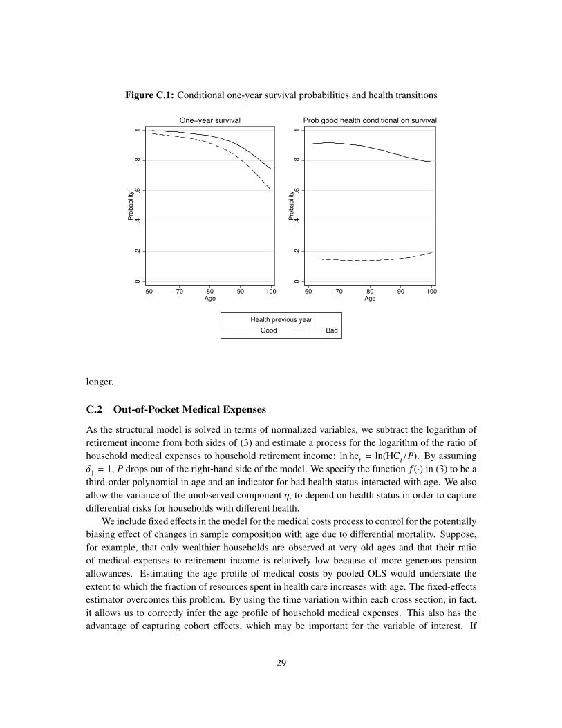
Figure C.1: Conditional one-year survival probabilities and health transitions

0.2

.4.6

.81

Pro

ba

bili

ty

60 70 80 90 100Age

One−year survival

0.2

.4.6

.81

Pro

ba

bili

ty60 70 80 90 100

Age

Prob good health conditional on survival

Good Bad

Health previous year

longer.

C.2 Out-of-Pocket Medical Expenses

As the structural model is solved in terms of normalized variables, we subtract the logarithm ofretirement income from both sides of (3) and estimate a process for the logarithm of the ratio ofhousehold medical expenses to household retirement income: ln hct = ln(HCt/P). By assumingδ1 = 1, P drops out of the right-hand side of the model. We specify the function f (·) in (3) to be athird-order polynomial in age and an indicator for bad health status interacted with age. We alsoallow the variance of the unobserved component ηt to depend on health status in order to capturedifferential risks for households with different health.

We include fixed effects in the model for the medical costs process to control for the potentiallybiasing effect of changes in sample composition with age due to differential mortality. Suppose,for example, that only wealthier households are observed at very old ages and that their ratioof medical expenses to retirement income is relatively low because of more generous pensionallowances. Estimating the age profile of medical costs by pooled OLS would understate theextent to which the fraction of resources spent in health care increases with age. The fixed-effectsestimator overcomes this problem. By using the time variation within each cross section, in fact,it allows us to correctly infer the age profile of household medical expenses. This also has theadvantage of capturing cohort effects, which may be important for the variable of interest. If

29

not appropriately accounted for, systematic differences in health care behavior among generationsmay lead to biased assessments of the age effect on household medical costs. The regressions alsoinclude year dummies, which pick up variations in medical prices that differ from inflation andvariations in medical costs due to other unmodeled causes, such as the business cycle.

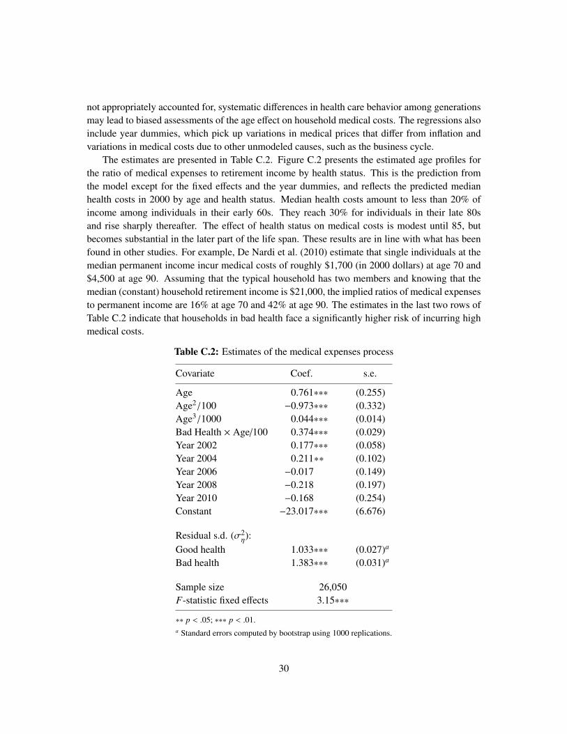
The estimates are presented in Table C.2. Figure C.2 presents the estimated age profiles forthe ratio of medical expenses to retirement income by health status. This is the prediction fromthe model except for the fixed effects and the year dummies, and reflects the predicted medianhealth costs in 2000 by age and health status. Median health costs amount to less than 20% ofincome among individuals in their early 60s. They reach 30% for individuals in their late 80sand rise sharply thereafter. The effect of health status on medical costs is modest until 85, butbecomes substantial in the later part of the life span. These results are in line with what has beenfound in other studies. For example, De Nardi et al. (2010) estimate that single individuals at themedian permanent income incur medical costs of roughly $1,700 (in 2000 dollars) at age 70 and$4,500 at age 90. Assuming that the typical household has two members and knowing that themedian (constant) household retirement income is $21,000, the implied ratios of medical expensesto permanent income are 16% at age 70 and 42% at age 90. The estimates in the last two rows ofTable C.2 indicate that households in bad health face a significantly higher risk of incurring highmedical costs.

Table C.2: Estimates of the medical expenses process

Covariate Coef. s.e.

Age 0.761∗∗∗ (0.255)Age2/100 −0.973∗∗∗ (0.332)Age3/1000 0.044∗∗∗ (0.014)Bad Health × Age/100 0.374∗∗∗ (0.029)Year 2002 0.177∗∗∗ (0.058)Year 2004 0.211∗∗ (0.102)Year 2006 −0.017 (0.149)Year 2008 −0.218 (0.197)Year 2010 −0.168 (0.254)Constant −23.017∗∗∗ (6.676)

Residual s.d. (σ2η):

Good health 1.033∗∗∗ (0.027)a

Bad health 1.383∗∗∗ (0.031)a

Sample size 26,050F-statistic fixed effects 3.15∗∗∗

∗∗ p < .05; ∗∗∗ p < .01.a Standard errors computed by bootstrap using 1000 replications.

30

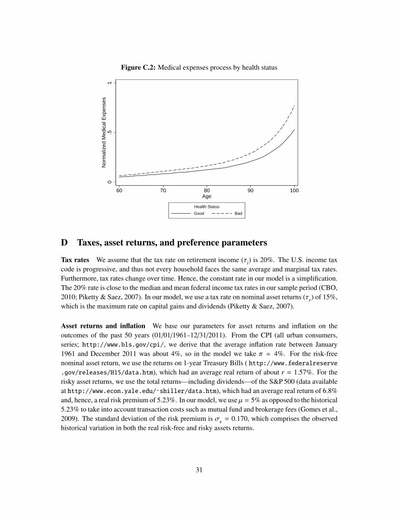
Figure C.2: Medical expenses process by health status

0.5

1N

orm

aliz

ed M

edic

al E

xpen

ses

60 70 80 90 100Age

Good Bad

Health Status

®

D Taxes, asset returns, and preference parameters

Tax rates We assume that the tax rate on retirement income (τi) is 20%. The U.S. income taxcode is progressive, and thus not every household faces the same average and marginal tax rates.Furthermore, tax rates change over time. Hence, the constant rate in our model is a simplification.The 20% rate is close to the median and mean federal income tax rates in our sample period (CBO,2010; Piketty & Saez, 2007). In our model, we use a tax rate on nominal asset returns (τr) of 15%,which is the maximum rate on capital gains and dividends (Piketty & Saez, 2007).

Asset returns and inflation We base our parameters for asset returns and inflation on theoutcomes of the past 50 years (01/01/1961–12/31/2011). From the CPI (all urban consumers,series; http://www.bls.gov/cpi/, we derive that the average inflation rate between January1961 and December 2011 was about 4%, so in the model we take π = 4%. For the risk-freenominal asset return, we use the returns on 1-year Treasury Bills ( http://www.federalreserve.gov/releases/H15/data.htm), which had an average real return of about r = 1.57%. For therisky asset returns, we use the total returns—including dividends—of the S&P 500 (data availableat http://www.econ.yale.edu/˜shiller/data.htm), which had an average real return of 6.8%and, hence, a real risk premium of 5.23%. In our model, we use µ = 5% as opposed to the historical5.23% to take into account transaction costs such as mutual fund and brokerage fees (Gomes et al.,2009). The standard deviation of the risk premium is σε = 0.170, which comprises the observedhistorical variation in both the real risk-free and risky assets returns.

31

Preference parameters Preference parameters are taken from previous studies using life-cyclemodels of saving and portfolio choice. In particular, the discount factor, β, is set to 0.96, as inCocco et al. (2005), and the coefficient of relative risk aversion, γ, is set to 4, as in De Nardi et al.(2010). In the text we also present results with γ = 1.5, which is closer to what Hurd (1989) andAttanasio and Weber (1993, 1995) find.

References

Alan, S. (2006). Entry costs and stock market participation over the life cycle. Review of EconomicDynamics, 9, 588–611.

Ameriks, J., & Zeldes, S. (2004). How do portfolio shares vary with age? Mimeo, ColumbiaBusiness School.

Attanasio, O. P., & Weber, G. (1993). Consumption growth, the interest rate and aggregation.Review of Economic Studies, 60, 631–649.

Attanasio, O. P., & Weber, G. (1995). On the aggregation of Euler equations for consumption insimple overlapping-generations models. Economica, 62, 565–576.

Banks, J., Blundell, R., Oldfield, Z., & Smith, J. P. (2010). Housing price volatility and downsizingin later life. In D. A. Wise (Ed.), Research findings in the economics of aging (pp. 337–379).Chicago, IL: University of Chicago Press.

Blau, D. (1994). Labor force dynamics of older men. Econometrica, 62(1), 117-156.Brent, R. P. (1973). Algorithms for minimization without derivatives. Englewood Cliffs, NJ:

Prentice-Hall. (Reprinted 2002 by Dover Publications, Mineola, NY)Campbell, J. Y. (2006). Household finance. Journal of Finance, 61, 1553–1604.Campbell, J. Y., Cocco, J. F., Gomes, F. J., & Maenhout, P. J. (2001). Investing retirement wealth a

life-cycle model. In J. Y. Campbell & M. Feldstein (Eds.), Risk aspects of investment-basedsocial security reform (pp. 439–482). Chicago, IL: University of Chicago Press.

Carroll, C. D. (1992). The buffer-stock theory of saving: Some macroeconomic evidence.Brookings Papers on Economic Activity, 1992(2), 61–156.

Carroll, C. D. (1997). Buffer-stock saving and the life cycle/permanent income hypothesis.Quarterly Journal of Economics, 112, 1–55.

Cocco, J. F., Gomes, F. J., & Maenhout, P. J. (2005). Consumption and portfolio choice over thelife cycle. Review of Financial Studies, 18, 491–533.

Coile, C., & Gruber, J. (2007). Future social security entitlements and the retirement decision.The Review of Economics and Statistics, 89(2), 234–246.

Congressional Budget Office [CBO]. (2010). Average federal tax rates in 2007.Washington, DC: Congressional Budget Office. Retrieved September 9, 2012, fromhttp://www.cbo.gov/sites/default/files/cbofiles/ftpdocs/115xx/doc11554/

averagefederaltaxrates2007.pdf

Curcuru, S., Heaton, J., Lucas, D., & Moore, D. (2010). Heterogeneity and portfolio choice:Theory and evidence. In Y. Aıt-Sahalia & L. P. Hansen (Eds.), Handbook of financialeconometrics (pp. 337–382). Amsterdam, Netherlands: North-Holland.

32

Deaton, A. (1991). Saving and liquidity constraints. Econometrica, 59, 1221–1248.De Nardi, M., French, E., & Jones, J. B. (2010). Why do the elderly save? The role of medical

expenses. Journal of Political Economy, 118, 39–75.Dominitz, J., & Manski, C. F. (2007). Expected equity returns and portfolio choice: Evidence

from the Health and Retirement Study. Journal of the European Economic Association, 5,369–379.

Eeckhoudt, L., & Kimball, M. (1992). Background risk, prudence and the demand for insurance.In G. Dionne (Ed.), Contributions to insurance economics (pp. 239–254). New York, NY:Springer.

French, E. (2005). The effects of health, wealth, and wages on labour supply and retirementbehaviour. Review of Economic Studies, 72, 395–427.

French, E., & Jones, J. B. (2004). On the distribution and dynamics of health care costs. Journalof Applied Econometrics, 19, 705–721.

Gomes, F., Michaelides, A., & Polkovnichenko, V. (2009). Optimal savings with taxable andtax-deferred accounts. Review of Economic Dynamics, 12, 718–735.

Gourinchas, P.-O., & Parker, J. A. (2002). Consumption over the life cycle. Econometrica, 70,47–89.

Guiso, L., Jappelli, T., & Terlizzese, D. (1996). Income risk, borrowing constraints, and portfoliochoice. American Economic Review, 86, 158–172.

Guiso, L., Sapienza, P., & Zingales, L. (2008). Trusting the stock market. Journal of Finance, 63,2557–2600.

Gustman, A. L., Steinmeier, T. L., & Tabatabai, N. (2010). Pensions in the Health and RetirementStudy. Cambridge, MA: Harvard University Press.

Haliassos, M., & Bertaut, C. C. (1995). Why do so few hold stocks? Economic Journal, 105,1110–1129.

Haliassos, M., & Michaelides, A. (2003). Portfolio choice and liquidity constraints. InternationalEconomic Review, 44, 143–177.

Heaton, J., & Lucas, D. (2000). Portfolio choice in the presence of background risk. EconomicJournal, 110, 1–26.

Hochguertel, S. (2003). Precautionary motives and portfolio decisions. Journal of AppliedEconometrics, 18, 61–77.

Hong, H., Kubik, J. D., & Stein, J. C. (2004). Social interaction and stock-market participation.Journal of Finance, 59, 137–163.

Hubbard, G., Skinner, J., & Zeldes, S. (1995). Precautionary saving and social insurance. Journalof Political Economy, 103, 360–399.

Hung, A. A., Meijer, E., Mihaly, K., & Yoong, J. (2009). Building up, spending down: Financialliteracy, retirement savings management, and decumulation (Working Paper No. WR-712).Santa Monica, CA: RAND Corporation.

Hurd, M. D. (1989). Mortality risk and bequests. Econometrica, 57, 779–813.Hurd, M. D. (1990). Research on the elderly: Economic status, retirement, and consumption and

saving. Journal of Economic Literature, 28, 565–637.Hurd, M. D. (2002). Portfolio holdings of the elderly. In L. Guiso, M. Haliassos, & T. Jappelli

33

(Eds.), Household portfolios (pp. 431–472). Cambridge, MA: MIT Press.Hurd, M. D. (2009). Subjective probabilities in household surveys. Annual Review of Economics,

1, 543–562.Hurd, M. D., & Rohwedder, S. (2011). Stock price expectations and stock trading. Mimeo, RAND

Corporation, Santa Monica, CA.Hurd, M. D., Van Rooij, M., & Winter, J. (2011). Stock market expectations of Dutch households.

Journal of Applied Econometrics, 26, 416–436.Juster, F. T., & Suzman, R. (1995). An overview of the Health and Retirement Study. Journal of

Human Resources, 30, S7–S56.Kezdi, G., & Willis, R. J. (2008). Stock market expectations and portfolio choice of American

households. Mimeo, University of Michigan, Ann Arbor.Kimball, M. S. (1990). Precautionary saving in the small and in the large. Econometrica, 58,

53–73.Korniotis, G. M., & Kumar, A. (2011). Do older investors make better investment decisions?

Review of Economics and Statistics, 93, 244–265.Lee, J., Kapteyn, A., Meijer, E., & Yang, J.-S. (2010). Pre- and post-retirement asset portfolios

(Publication No. 213). Madison, WI: Filene Research Institute.Lockwood, L. M. (2012). Bequest motives and the annuity puzzle. Review of Economic Dynamics,

15, 226–243.Merton, R. C. (1969). Lifetime portfolio selection under uncertainty: The continuous-time case.

Review of Economics and Statistics, 51, 247–257.Paiella, M. (2007). The forgone gains of incomplete portfolios. Review of Financial Studies, 20,

1623–1646.Piketty, T., & Saez, E. (2007). How progressive is the U.S. federal tax system? A historical and

international perspective. Journal of Economic Perspectives, 21(1), 3–24.Rosen, H. S., & Wu, S. (2004). Portfolio choice and health status. Journal of Financial Economics,

72, 457–484.Samuelson, P. A. (1969). Lifetime portfolio selection by dynamic stochastic programming.

Review of Economics and Statistics, 51, 239–246.Scholz, J. K., Seshadri, A., & Khitatrakun, S. (2006). Are americans saving “optimally” for

retirement? Journal of Political Economy, 114, 607–643.St.Clair, P., et al. (2011). RAND HRS data documentation, Version L. Santa Monica, CA: RAND

Corporation.Vissing-Jørgensen, A. (2002). Limited asset market participation and the elasticity of

intertemporal substitution. Journal of Political Economy, 110, 825–853.Yogo, M. (2009). Portfolio choice in retirement: Health risk and the demand for annuities,

housing, and risky assets (Working Paper No. 2009-3). Chestnut Hill, MA: Center forRetirement Research at Boston College.

34