Investment, Capacity Utilization, and the Real Business · PDF fileInvestment, Capacity Utilization, and the Real Business Cycle By JEREMY GREENWOOD, Zvi HERCOWITZ, AND GREGORY W

Investment, Capacity Utilization, and the Real Business Cycle

By JEREMY GREENWOOD, Zvi HERCOWITZ, AND GREGORY W. HUFFMAN*

This paper adopts Keynes' view that shocks to the marginal efficiency of investment are important for business fluctuations, but incorporates it in a neoclassical framework with endogenous capacity utilization. Increases in the efficiency of newly produced investment goods stimulate the formation of "new" capital and more intensive utilization and accelerated depreciation of "old" capital. Theoreti- cal and quantitative analysis suggests that the shocks and transmission mechanism studied here may be important elements of business cycles.

In the real-business cycle models of the type developed by Finn Kydland and Ed- ward Prescott (1982), and John Long and Charles Plosser (1983), the cycles are generated by exogenous shocks to the production function. A stylized version of the main mechanism working in these models can be described as follows. Dynamic optimizing behavior on the part of agents in the economy implies that both consumption and investment react positively to these direct shocks to output. Since the marginal productivity of labor is directly affected, employment is also procyclical. The resulting capital accumulation provides a channel of persistence, even if the technology shocks are serially uncorrelated. Hence, these productivity shocks are able to generate, from a neoclassical framework, co-movements of macroeconomic variables and persistence of fluctuations that conform to those typically observed during business cycles.

In contrast with the mechanism described above, where investment reacts to changes in output, the present paper adopts John Maynard Keynes' (1936) view that it is shocks to the marginal efficiency of investment that are important for generating out-

put fluctuations. However, these shocks are incorporated here in a neoclassical framework where the rate of capital utilization is endogenous. In the present model, a positive shock to the marginal efficiency of investment stimulates the formation of "new" capital and the more intensive utilization and accelerated depreciation of "old" capital. The main operating characteristics of the proposed model are analyzed in order to gain an understanding of the transmission mechanism of the shocks. Of particular theoretical interest are the qualitative characteristics of the pattern of co-movements and persistence effects permissible in this framework Then, a quantitative analysis of the model is performed to assess its ability to mimic the observed pattern of postwar-U.S. business cycle fluctuations. This is carried out by constructing a parametrized version of the model for which the exact joint probability distribution of the endogenous and exogenous variables is numerically computed. Using this distribution, a set of second moments for the artificial economy's variables-reflecting their co-movements and persistence-is computed and compared with that characterizing U.S. data.

Fluctuations in investment played a key role in Keynes' view of the trade cycle. There, shifts in the marginal efficiency of investment impact on investment, aggregate demand and therefore, given the disequi- librium in the labor market, employment and output. The quintessential case of this type is when there is an increase in the

*Department of Economics, University of Western Ontario, London N6A 5C2, Canada; Department of Economics, Tel Aviv University, Tel Aviv 69978 Israel; Department of Economics, The University of Western Ontario, London N6A 5C2 Canada. The authors thank Finn E. Kydland, Edward C. Prescott, Thomas J. Sar- gent, Lars E. 0. Svensson, and two anonymous referees for their helpful comments.

402

VOL. 78 NO. 3 GREEN WOOD ET A L.: REA L B USINESS C YCLE 403

marginal efficiency of newly produced capital that does not affect the productivity of the capital stock already on line. When a shock of this type occurs in a standard neoclassical model, employment and output also tend to rise, but the mechanism is very different. The increase in the rate of return on investment stimulates current labor effort and output through an intertemporal substitution effect on leisure. A potential problem with this mechanism, as discussed by Robert Barro and Robert King (1984), is that intertemporal substitution which induces individuals to postpone leisure, also works to cut consumption. This effect would tend to make consumption move countercyclically, which contradicts the evidence. Labor productivity would tend to move in the " wrong" direc- tion, too. An expansion of labor effort, given the fixed supply of capital in the short run, causes labor's productivity to decline.

In contrast to the intertemporal substitution effect mentioned above, the transmission mechanism of the investment shocks works in the present model through the optimal utilization of capital and its positive effect on the marginal productivity of labor. As will be seen, an important aspect of such a change in labor productivity is that it creates intratemporal substitution, away from leisure and toward consumption, generating procyclical effects on consumption and labor effort. Additionally, average labor productivity responds procyclically to these shocks.

To sharpen the distinction between this and the real business cycle models with direct shocks to the production function, no shifts of the latter type are included. There- fore, given the quantities of capital and labor input, current productivity shifts are endogenous in this framework. The shocks to investment are modeled as current technological changes that affect the productivity of new capital goods only, leaving unchanged the productivity of the existing capital. Be- cause of a time-to-build delay, only the productivity of future capital is affected. This type of technological change may be more realistic than the current shock to productivity. Important technological improvements of new productive capital seem to occur quite often. As will be discussed, it is crucial

for this model that the new technology does not affect directly the productivity of the existing capital stock.

A description of the environment characterizing the economy under study is given in Section I. In Section II the representative agent's optimization problem is cast. The theoretical investigation of the model is carried out in Section III, and the quantitative analysis in Section IV. Finally, concluding remarks are offered in Section V.

I. The Economic Environment

Consider a perfectly competitive closed economy populated by a very large number of identical households and identical firms. Aggregate output is given by the following constant-returns-to-scale production function which differs from the standard neoclassical specification solely by the inclusion of a variable rate of capital utilization

(1) yt = F(kthtg It),

where y, is the output of the single good in period t, k, is the capital stock (see below for a discussion about its units) at the beginning of period t, h, is an index of the period-t utilization rate of k,, and It is labor input in this period. The variable h -which for a given capital stock determines the flow of capital services kth -represents the in- tensity of the use of capital, that is, the speed of operation or the number of hours per period the capital is used. An alternative interpretation of h, is that while It represents the total labor employed, h, reflects the portion of it used directly in production, with the remainder being involved in maintenance activities. The nonnegative, constant- returns-to-scale function F satisfies F1, F2 > 0, F11, F22 < 0, and F11F22 - 2F1 = 0. A consequence of the constant-returns-to-scale assumption is that F12> 0, which implies capital and labor services are complements in the Edgeworth-Pareto sense. This feature provides a positive link between capital utilization and labor productivity.'

'A special case would be one of fixed proportions where, for a given k,, h, and l, should move together.

404 THEAMERICAN ECONOMIC REVIEW JUNE 1988

The capital utilization decision involves Keynes' notion of "user cost." That is, a higher utilization rate causes a faster depreciation of the capital stock, either because wear and tear increase with use or because less time can be devoted to maintenance.2 As in the work of Paul Taubman and Maurice Wilkinson, 1970; Guillermo Calvo, 1975; John Merrick, 1984; and Zvi Hercowitz, 1986, this effect is modeled in the evolution of the capital stock as

(2) kt+i =kt[1 -8(hj)]+ it(1 +,Et)

where the nonnegative depreciation function 8 satisfies 0 < 8 < 19 8'> 09 '" > 0. Gross investment, as corresponding to the national income accounts, is it. Its contribution to the production capacity in t +1, however, depends on the technological shift factor Et, affecting the productivity of the new capital goods. The productivity of the already in- stalled capital stock k, is not directly affected by the new technology. Correspondingly, k?t+ is a measure of the future capital stock in productivity units. (Similarly k, would include past technological changes.)

Note that this technological disturbance is very different from the usual technological shock, attached to the production function, used in the real business cycle models. By substituting k,+1 into the production function corresponding to t + 1, it becomes clear that Et works as a shift in the marginal efficiency of capital produced in period t which comes on line in t + 1. The length of the basic period, which corresponds to the time-to-build, is thought of as nontrivial, say one year (see the discussion in Kydland and Prescott, 1982).

The value of Et, which is realized at the beginning of period t, is generated from the stationary Markov distribution function t(eD (-,1) defined on the domain Q = [E, E].

The assumption that Et is stationary implies in the present framework, that the equilibrium capital stock will also be stationary.

The representative household in this economy maximizes expected lifetime utility as given by

(3) Eo E U t 0 t < 8 < 19

_ t = 0

where c, and It are the period-t flows of consumption and labor effort, and / is the discount factor.

The specific form of U adopted is

U(ct, It) = U(c, -G(IJ)

with U'> O, U" < O, G' > O, and G" > O, and where U is assumed to be bounded from above. This utility function satisfies the standard properties U1 > O, 2 <0, U09 , U22 <O,U11 U22 -U > 0, and it implies that the marginal rate of substitution between consumption and labor effort depends on the latter only:

E2 (Ct , 't)

That is, labor effort is determined independently of the intertemporal consumption- savings choice, which is very convenient in obtaining results from the model. As a consequence, the intertemporal substitution effect on labor effort, a central ingredient in many macroeconomic models, is eliminated. Rather than being a drawback, this implica- tion of the utility function has the advantage of emphasizing the alternative transmission of investment shocks being studied here. When analyzing fluctuations in labor effort, this framework stresses shifts in the productivity of labor brought about by changes in the optimal rate of capacity utilization, as opposed to intertemporal substitution effects stressed by others.

The description of the setup is completed by the resource constraint

(4 t=C AX

i,

2Keynes said: "User cost constitutes the link between the present and the future. For in deciding his scale of production an entrepreneur has to exercise a choice between using up his equipment now or preserv- ing it to be used later on..." (1936, pp. 69-70) [quoted also by Taubman and Wilkinson, 1970].

VOL. 78 NO. 3 GREENWOOD ETAL.: REAL BUSINESS CYCLE 405

II. The Representative Agent's Optimization Problem

The decision making of consumer-workers and firms in competitive equilibrium can be summarized by the outcome of the following " representative" agent's dynamic-programming problem

(5) V(kt; Et)= max lU(ct, It) (c,, k, + , h,t, It)L

+ 13f V(kt+?; e_t+?) d0(t+jjEt) 9

subject to

(6) ct = F(kth t, It) -

I t I t

x [I1- 8(ht)] ,

where the transition equation (6) is obtained by substituting the production function (1) and the capital evolution equation (2) into the resource constraint (4).3'4 It can be established that the value function V(.;-) exists, is unique, increasing, concave, and differentiable in its first argument (see

Robert Lucas, Edward Prescott, and Nancy Stokey, 1985).

The solution to the above programming problem is characterized by the following three efficiency conditions-in addition to (6)

(7) U'(c -G (I,))/(1 ? Et)

- f3f V1(kt?1; Et+1) dF( Et?iIet)

= |U'(c,+,-G(It+,))

x [Fl(kt+lh t+ 1, lt+l)ht+l

? (1- 8(h t+))/(I + Et+?J]

x d ?D( -t+ll,-t) -

(8) F1(ktht, it) = 8'(ht)/(1 + E).

(9) F2(ktht, It) = G'(1t).

The first equation (7) is a standard optimality condition governing investment. The left-hand side of this equation represents the loss in current utility which is realized when an extra unit of current investment is undertaken. The right-hand side portrays the dis- counted expected future utility obtained from an extra unit of investment today. Note that an increase in the investment technological shift factor, (1 + Et), reduces the utility cost of an extra unit of capital accumulation in this period. This occurs because a given increase in expected future output can now be obtained with a lower amount of current investment.

The next equation (8) characterizes efficient capital utilization. It states that capital should be utilized at the rate, hp, which sets the marginal benefit of capital services equal to the marginal user cost. The marginal user cost of capital is made up of two compo- nents. Specifically, 8'(h ) represents the marginal cost in terms of increased current depreciation from utilizing capital at a higher rate, while 1/(1 + Et) is the current replace- ment cost of old in terms of new capital.

3The functions F( ),8( ), U(-), and G(-) are all assumed to be twice continuously differentiable.

4Note that the capacity utilization variable, h, could be eliminated from the above programming problem by utilizing the production function defined by

cp(k,l,E) = max F(kh,l)+ k(I -(h))]

It is easy to establish that 0(.) is well-behaved in the usual sense of being jointly concave in k and 1, etc. Of interest is the fact that while a technological improve- ment increases the marginal product of labor, it de- creases that of capital. Thus, E does not operate here in the manner of standard Hicks or Harrod-neutral technological shock. Using this production function, equation (6) can be rewritten as

k+1

Ct = 0( kt lt Et (1?)'

which does not involve h,

406 THE AMERICAN ECONOMIC REVIEW JUNE 1988

Finally, equation (9) sets the marginal product of labor equal to the marginal disutility of working, measured in terms of consumption. Again, given the form of the utility function adopted, the latter depends only upon current labor effort, and thus is determined independently of the agent's intertemporal consumption-savings decision. The advantage of this characteristic is that the system of equations (6)-(9) is recursive in the sense that (8) and (9) jointly determine ht and 4, while then given these solutions equation (7)-in conjunction with (6)-determines the intertemporal allocation, which amounts here to specifying values for kt+? and ct.

1II. Qualitative Analysis of the Model

An analysis of the effect of the technology shift Et governing the marginal efficiency of investment, on output, hours worked, capacity utilization, productivity, investment, and consumption will now be undertaken. For simplicity, the discussion in this section is carried out under the assumption that the disturbances are purely temporary-that is, independently distributed over time, so that I ( Etc+llt? ) = ID(Et+l). This serves two purposes: first, it allows for clear results to be obtained, and second, it emphasizes the main characteristics of the model's propagation mechanism.

A. Impact Effect of Investment Shocks

The endogenous capital utilization is central to the model's ability to generate positive co-movement of investment, productivity, and consumption. In a neoclassical model of the present type but with constant capital utilization (and a general utility function), shocks to the productivity of investment would have different effects. A positive shock, for example, would tend to generate intertemporal substitution, away from current consumption and toward current investment and future consumption. The higher return on currently available resources would, at the same time, operate to persuade individuals to postpone leisure. Additionally, the resulting expansion in labor effort and out-

put would lead to a decline in labor productivity, given the fixed stock of capital in place. Thus, investment and output would move inversely with consumption and productivity in response to these shocks. (A formal discussion of the above is provided in the Appendix.)

Given the structure of the optimality conditions (7)-(9), the effect on the variables, ht, It, yt, and productivity, can be calculated from (8) and (9) only. Performing the standard comparative statics exercise on (8) and (9) yields

(10) d S=- )22 ( t )-G

[(1 + )2g(t) > 0,

(11) d F12(t) ktS (t)/

[(1 + Et)2 &(t)] > 0,

with

Qi(t) -Fl,(t)ktG"(t)-8"(t)

X [F22(t) - G"(t)/(1l + Et) >0,

where the sign restriction follows from the concavity of F(.), and the convexity of 8(.) and G(.).

The interpretation of these results is that Et reduces the cost of capital utilization and hence induces a higher h,. Since F12 > O, labor's marginal productivity increases, resulting in a higher level of employment.5

5A labor market interpretation of these results is the following. Letting w, represent the period-t real wage, equilibrium in the labor market for this period can be characterized by the condition ld(k,h,, w,) = Ps(w,), where the labor demand function ld(t) solves the equation F2(k,h,, ld(k,h,,w,))=w, and the labor supply function, PS(t), is given by PS = G'-1(wt). Clearly, increased capacity utilization induces a positive shift in labor demand which necessitates equilibrating increases in both the real wage and labor supply. By contrast, in the conventional model with time-separable preferences and with constant capacity utilization-see Barro and King, 1984-the period-t labor market-clearing condition would be represented by an equation of the form Id(k,, w,) = P(w,, rt, a,), where rt represents the known period-t real interest-on one-period bonds maturing in period t + 1-and a, agents' real wealth net of labor

VOL. 78 NO. 3 GREENWOOD ETAL: REAL BUSINESS CYCLE 407

Given that kt is predetermined, (10) and (11) immediately imply a positive output effect. The increase in capital utilization implies that labor productivity also rises. Using (10) and (11) it is easy to establish that the marginal product of labor F2(k,h,, 4t), moves upward. Specifically, one finds

d2 ( t)0 = [F12(t)k,3'(t)G"(t)I/

|(I+ -t)223(t)] > O.

Given the constant-returns-to-scale assumption, the average product of labor, F(ktht, t)/1t, also must rise.6

The impact effects of the investment shock, et, on next period's capital stock, kt+1, and current consumption, ct, are deduced by dis- placing the system of equations (6) and (7) while making use of the first-order conditions (8) and (9). The resulting expressions are

(12) de, - U'(t)

W[u (t)+ 3( + E,t)2 Vll(t + 1) doj

u"(t) + it --.

U"(t) + fi(1 + et)2f Vll(t + 1) dIj

> 0,

and

dct F2(t)ktFl2 (t )8 (t) (13) -

de t (l + Et)20(t )

U'(t)/(1 + Et) + . ~ 2 ./( 1)

u (1 + ( t)2f V11(t + 1) d(I

9(1+et)| Vll(t+l) d(

U (t) + ?(1 + et)2f VI,(t + 1) d(j

><O.

Note that these formulas presume that V(-) is a twice continuously differentiable concave function in k, whereas actually it can only be shown that V(-) is continuously differentiable and concave.7 An argument analogous to that used by Thomas Sargent (1980) can be used to show, though, that since V(-) is concave the sign restrictions in equations (12) and (13) continue to hold if these expressions are suitably reinterpreted as representing finite differences instead of derivatives.

As can be seen from (12), the technology shock, Et, has two effects on the period-t + 1 capital stock. The first term illustrates the positive substitution effect that an increase in the productivity of newly produced capital has on the period-t +1 capital stock. The second term represents the income effect associated with the shock, which is positive if it > 0. A given desired level for next period's capital stock can now be obtained with a lower level of current investment. Consump- tion-smoothing agents will utilize part of this savings in current resource utilization to increase the future stock of capital.

Current consumption is affected in three ways by a movement in t (compare (13)). The second term, which is negative, il-

income in this period. Here the impact of a shift in the technology factor e, affects the current level of employment and the real wage via the intertemporal substitution effect on labor supply excerted by the induced shift in the real interest rate, rt. (It should perhaps be empha- sized that w,, rt, and at in equilibrium will all be functions of the current state of the world.)

6This can be shown as follows. The marginal product increases if and only if the capital to labor services ratio, k,h,/l,, also increases, since F2(kth,, 1,) = F(k,h,/ll,1) - (k,ht/l,)Fl(k,h,/l,,1). This is relevant since the average product F(k,h,, 1,)/1, can be expressed as a strictly increasing function of k,h ,/l: F(k,h,, ,t)/l, = F(k,h,/l,,1). Therefore, average productivity also moves procyclically.

7The agent's choice set is convex since the production function p ( k, 1, E) (see fn. 4) is concave. Therefore, standard dynamic programming arguments establish the concavity of the value function.


lustrates the intertemporal substitution effect associated with the improved productivity of newly produced capital. The increase in the rate of return on current investment operates to dissuade consumption and promote capital accumulation. The income effect associated with this technological change, which was explained above, works to raise current consumption and is represented by the third term. The standard macroeconomic pre- sumption is that the intertemporal substitution effect generated by such technological shift will dominate the income effect, a situa- tion ensured if the initial level of investment is small enough. The new element that the present model introduces is the first term, which has to do with the intratemporal margin of substitution between consumption and leisure. This effect may be interpreted as follows. Since F12 > 0 a higher utilization rate increases the marginal productivity of labor, which represents the opportunity cost of current leisure in terms of consumption. This generates a substitution effect, away from leisure and toward consumption. Hence, the present model provides a channel by which both consumption and investment can possibly react procycically.

Finally, the impact effect on gross investment, it, is given by

(14) t K 1 +

[dkt+1 dh 1 X I -it+ 3'(t)kt .

d,Et dE t

The first two terms loosely represent oppo- site "substitution" and "income" type effects. If the initial it is relatively small, the substitution effect will clearly dominate. Here there is another positive effect on gross investment coming from the additional depreciation term 8'(t)ktdht/deF.

The results obtained so far depend cru- cially upon the assumption that the technological shift pertains only to newly produced capital goods. Suppose alternatively that it applies both to newly produced, it, and existing capital, [1 - 8(ht)Ikt. Then, equation

(2) governing the evolution of capital becomes

kt+l =1 kt [1- 8(ht)](l + Et) + it(l + Et),

and the transition equation (6) now becomes

k Ct =F(ktht, I t)- + + kt [1- 8(ht)].

t

While the form of the efficiency conditions (7) and (9) characterizing the optimal choices for kt+1 and It remain unchanged, equation (8) specifying the optimal level for ht is significantly altered to

F1(ktht, It) = 8 (ht)-

Since the productivity term, et, no longer enters the system of equations (8) and (9) now, the positive effects of a technological shift on ht, 4t, yt, and productivity, in addition to the procyclical effect on consumption, are all lost. This result obtains since it not longer pays to depreciate "off" old capital through higher levels of utilization.

B. Dynamic Effects of Investment Shocks

Under the assumption made that Et is serially uncorrelated, the only channel through which persistence can be generated is kt+l,. In the standard paradigm, a higher kt+1 implies more capital services, which directly tends to prolong the initial effects. In the present model, where the utilization is endogenous, higher capital does not obvi- ously mean higher capital services. Whether there are prolonged output effects depends on how kt+ 1 affects decisions at t + 1, and in particularly capacity utilization. Since the state of the world has yet to materialize, the goal here is to discern how the increase in current capital accumulation, induced by the technology shock, impacts on the means of the distributions of future endogenous variables.

From the optimality conditions (8) and (9) corresponding to period-t + 1, it follows that for any given realization of the period-t +1

VOL. 7R NO ? GREENWOOD ETAL.: REAL BUSINESS CYCLE 409

technology shock

(15) = -Fll(t+l)ht+ kt+

x [F22(t + 1)-G"(t + 1)]

+ F12(t + 1)2ht+l }/s2(t + 1)

<0,

and

dlt+ (16) S"(t + 1)F12(t+l)ht+]l]

(1?+ Et?1)u(t + 1) > 0,

with the signs of the above expressions following from the facts that 2, F12> 0, and F is concave. The optimal rate of utilization declines since the higher kt+l reduces the marginal productivity of capital services ceteris paribus. However, this is only a partial offsetting. The optimal flow of capital services kt+ lht+?1 increases

(17) d(kt+ht+l)

dkt+l

dht+? = ht+1 + kt+1

=-ht+ ha18(t + 1)

xV[22( t+ 1) -G"(t + 1)]/

[(1 + Et+l)Q(t + 1)]

>0.

From (16) and (17) it follows that dy,?1/ dkt+l > 0, for any given value of et+1. The effects will persist also beyond t + 1 because from equation (7) and the first-order conditions (8) and (9) updated one period it transpires that

(18) dkt+2

dkt+ I

U"(t + 1) {(1 + E,+i)FI(t + 1)h,+t + [1-8(t + 1)]}

U"(t +1)+?I(1+ e+)2fVll(t+ 2)dcD

> 0.

Finally, to see how the expected values of the period-t +1 endogenous variables are affected by a period-t technology shock note that these variables are functions of the period-t +1 state of the world-indeed this fact has been already repeatedly used- so that one can write policy functions of the form x `2= x(k?1+,cE?i) for x= h, 1, hk, and y. It immediately transpires that Et[xt+ ] = JQX(kt+?, t+ ?) dO()et+?1) from which it follows that dEtjxt+,I/dkt+1= Et[dxt+l/dkt+,]. Thus, by taking expected values of the above expressions it obtains that period-t +1 labor supply, capital services, output, and period-t +2 capital stock all rise in expected value, while expected-t + 1 capital utilization falls. The effects persist in similar fashion into the future periods, t + 2,....

The preceding analysis of the impact and dynamic effects of investment shocks was carried out under the assumption that -t is serially uncorrelated. The results about the impact effects on ht, I, and hence on current output are unchanged if -t is not serially independent. Note that equations (8) and (9), determining h, and 4, involve only Et, and not its future values, and hence, for these variables the serial correlation properties of Et are not relevant. However, it turns out that if Et is serially correlated, then it is not possible to sign dkt+l/dct unambigu- ously anymore.

The analysis carried out so far has shown that, theoretically, the model has potential for explaining the characteristics of business cycles. It suggests that it may be fruitful to incorporate jointly the rather Keynesian no- tions of shocks to the marginal efficiency of investment and variable capacity utilitzation into real-business cycle models. While the results obtained so far are illustrative, little light on their practical importance has been shed. Hence, a quantitative analysis of the model is now turned to with the purpose of evaluating its empirical relevance.

IV. Quantitative Analysis of the Model

In this section the model is suitably parameterized, calibrated, numerically solved, and evaluated. The exact nature of

410 THE A MERICA N ECONOMIC RE VIE W JUNE 1988

the experiment being proposed is this: First, a parametric representation of the model is obtained. Second, values for the various taste and technology parameters are chosen using information from either the literature or U.S. data. Third, by varying the parameters governing the stochastic structure of the sample economy, the model is calibrated so that it yields the same standard deviation and first-order autocorrelation coefficient for output as is displayed by U.S. data. Hence, the idea is to calibrate the model to mimic the behavior of output only, both in the terms of the volatility and persistence of its fluctuations. Fourth, the model is evaluated by comparing the generated standard deviations, serial correlations, and cross correlations with output of the other variables (consumption, investment, hours, and productivity) with the corresponding statistics in the U.S. data. It should be mentioned that in undertaking the above experiment the exact stationary joint distribution for the sample economy's state variables-the capital stock and the technology shock-is numerically computed so that the (population) second moments in question can be calculated.

A. Sample Economy and Solution Technique

To begin with, let tastes and technology be specified in the following way:

U(C,I) = 1l[(c- l

F(kh, 1) = (kh)alla,

1 and 6(h)= h-,

where y, 9 > 0, 0 < a <1, X >1. Next, suppose that the stochastic structure of the environment is described by a two-state Markov process. Specifically, in any given period the technology shock, E, is assumed to have a value lying in the time-invariant two-point set

E= fueti-,eo 2 v-e1 ng

The distribution function governing the

drawing of a value for next period's technology shock, ?', conditional upon a realized value for the current shock, E, is defined by

prob E' ec t- IIE = ec, - 1]- rs

where

0 < J,r <1, and 7Trl + 7Tr2=l1

for r, s =1,2.

The long-run (or unconditional) distribution function for the technology shock, associated with the above conditional distribution specifying the one-step transition probabilities between states, is given by8

(19) prob[e = ets-1] 4s*

qTrs

712 + 7T21

for r, s =1,2 and r # s.

Finally, it will be assumed that the capital stock in each period is constrained to be an element of the finite time-invariant set K = { k1, . . ., k,,}. Thus, the state space K X E for this economy will be discrete; a similar discretization procedure has been utilized by Sargent (1980). A discussion about the as- signment of values for the model's parameters-y, 6, /,I a, , the nT's, the c's, and the n elements of the set K -will be postponed until later.

The representative agent's dynamic-programming problem for the above setting can be expressed as

(20) V(ki; r)

=-max {i[c-l?)1

k zKi 1 c 8

2

+ 2 YE rsV(k'; (s) s=1

s.t. c k( +kkh ( -

-e- + ki 1--

hw

t

8See fn. 10 for a discussion of how these probabilities are determined.


where

h, I = argmax [(kih) al-/

-k (1 _h)e-- i w ~ 1+0

Hence, h and 1 can be solved first in terms of k and E, reducing the dynamic problem to one of choosing only k', the next period's capital stock.

The above problem can be solved numerically using standard algorithms discussed by Dimitri Bertsekas (1976). These algorithms are based on the fact that functional equations such as (20) describe contraction map- pings. This implies that iterative procedures, such as the one described below, can be used to solve numerically for the value function, V(.), over each of the 2n possible points in the state space, K x E; that is, for a value of V(kp, {r) for each possible combination of ki and (r. To begin with, an initial guess for the value function, V?(-), is made, say V?(ki, (r) = 0 for each i 1,...,n and r = 1,2. This initial guess for V(*) is used on the right-hand side of (20) and the optimized value of the maximand, which represents the left-hand side of the equation, is used as a revised guess, or V1(.). Then, V1(.) is entered into the right-hand side of (20) and the whole procedure is repeated until the agents' decision rules-here k'= k'(k, e)-have con- verged. Convergence of the decision rules is generally faster than for the value function, the latter whose solution is generally of no intrinsic interest for the problem being analyzed (see Bertsekas, 1976, p. 245).9

From the solution to the above-programming problem the long-run or asymptotic joint distribution function of the technology shock and the equilibrium capital stock can be obtained. To see how this is done, note that the solution for next period's capital stock, k', is such that given an initial capital

stock, ki, and a value for the technology shock, (r' a unique value for k'= k'(ki, ,r) E K will be chosen. Thus the probability prob[k'= kj1k = ki, = r will equal one for some j E {1,... ., n} and will be zero for the rest, where trivially then

n

E2 prob[k =kjIk=ki,= rI =1

forall(k, )e KxE.

Accordingly, the transition probability Pir,js of moving from the state characterized by capital stock ki and shock (r to the one represented by kj and 4, can be expressed as

Pir, s prob[k' = kjlk = ki, t-(rI grs

Vi, j=1,...,n.

V r,s =1,2.

Next the 2n X 2n transition matrix P with elements Pir,js is formed. Now suppose one is arbitrarily given some initial probability distribution over the permissible values of the capital stock and technology shock. Such an initial probability distribution will be represented by the 1 x 2n vector p?, specifying a probability p? that the initial capital stock/ technology shock combination is (ki, 0 for each i and r pair. The probability distribution, p1, governing next period's capital stock/technology shock combination is simply given by the mapping p1 = p?P. Assum- ing this finite state Markov chain model possesses a unique asymptotic joint distribution for the capital stock and technology shock, it can then be shown that iterations on this mapping must converge to a unique fixed point, p*, which satisfies p* = p*P.10 This is true for all initial distributions p?.

9In practice this iterative scheme can be accelerated using variations on the algorithm which are outlined in Bertsekas (1976).

loSimilarly, one could define H as the 2x2 transition matrix associated with the technology shock whose elements are the -rn5's. The unique steady-state distribution function associated with the technology shock, 0*, therefore solves the equation O* =4O*J. It is easy to deduce that the solution to this expression is given by formula (19).


Once the stationary joint probability distribution function for the capital stock and technology shock is known, it is easy to calculate various population moments of interest for the model. Note that all of the model's endogenous variables can be uniquely expressed as functions of the current capital stock and the state of technology, so that one may write x = x(k, () for x = c, k', h, 1, y, etc. Thus, for instance, the stationary moments for y, cy, and y'y can be written as

2 n

E[y]- = pi*y(ki,r r=1 i=1

2 n

E[cy]- = , pi*rc(ki, Oy(ki, 0 r=l1 i=

2 n 2 n

E [y'y] E E E 5? Pir, js s=1 j=1 r=1 i=1

xP* y'(kj, (s) y(ki ,r

B. Calibration Procedure and Results

The model to be used for the applied general-equilibrium analysis is patently sim- plistic; severe restrictions have been imposed on the forms of tastes, technology, and particularly on the stochastic structure of the economy. It will be interesting to see, therefore, how such a stylized artificial economy will be able to mimic the salient features of U.S. business cycles.

Before proceeding, the time length of a period in the model has to be defined. Given that the shocks represent technical innova- tion in the production of new capital goods, it seems appropriate to consider annual intervals since the frequency of such develop- ments is very unlikely to be higher. Also, the use of annual data has the advantage of avoiding seasonality issues.

Values for the model's tastes and technology parameters were chosen in the following manner. Two of the parameters could be assigned numbers straightforwardly. Follow- ing Kydland and Prescott (1982), the discount factor, /B, was specified to be .96.

Next, capital's share of national income had an average annual value of .29 over the 1950-85 period, so this value was picked for a.

The value of 1/0 corresponds to what in the literature is called the intertemporal elasticity of substitution in labor supply. Since the present model is based on a representative household, the empirical counterpart of 1/0 should summarize the variation in labor supply of all members of such a unit, both at the intensive and extensive margins. An estimate of this type, however, is not available. For adult males, Thomas Macurdy (1981) obtained estimates of about .3. From James Heckman and Thomas Macurdy (1980, 1982) the corresponding value for females is about 2.2. The first study refers to the intensive margin only (and does not include men younger than 25 years, who are likely to have higher variability in labor supply). The much higher estimate for females reflects both margins and therefore perhaps is more appropriate for current purposes. Hence, within the .3-2.2 range 1.7 was taken as a reasonable value, implying 9 =.6. Some analysis of the sensitivity of the results to the value of this parameter was carried out.

The empirical magnitude of the coefficient of relative risk aversion, y, is somewhat con- troversial. Therefore two alternative values, y = 1.0 (actually y = 1.001) and y = 2.0, were used. The first is close to the values found by Lars Hansen and Kenneth Singleton, 1983, and the second in accord with the estimates of Irwin Friend and Marshall Blume (1975).

The literature does not provide any guide for assigning a magnitude to X -the elasticity of depreciation with respect to utilization. The value of 1.42 was chosen for this parameter because, given the above value for /B, it implied a depreciation rate of .1 in a deterministic steady state for the model. This is the depreciation rate used by Kydland and Prescott.

The only "free" parameters are those de- limiting the stochastic structure of the model. To make things more manageable, let 11 =

722 = q7, and 41 = - 42 = a. It is easy to check that the asymptotic standard deviation and the first-order autocorrelation coefficient as-


Probability

0.030

0.025 -

0.020

0.016

0.010

0.006

0.000 0 10 20 30 40 50 60 70 80 90

Capital Stock

FIGURE 1. MARGINAL PROBABILITY DENSITY FOR CAPITAL

sociated with the shock, {, are given by a and X = 2r - -1, respectively. Thus, there are two free parameters to choose regarding the shock: its standard deviation, a, and first- order autocorrelation coefficient, A. As mentioned above, these parameters are to be determined so that the model generates the same standard deviation and first-order serial correlation for output as is observed in the data.

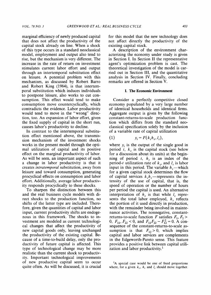
Finally, an evenly spaced grid of admissi- ble capital stock values was chosen, which captures the ergodic set of capital stocks linked with the stochastic steady state. The grid was refined until further subdivisions did not numerically affect the covariance structure of the endogenous variables. For instance, a grid of 90 evenly spaced capital stock points spanning the interval [0.470, 0.667] turned out to be sufficient for the case where -y = 2; the expected value of the capital stock in the stochastic steady state was 0.569 with a standard deviation of 0.032. The resulting unconditional probability density obtained for the capital stock is shown in Fig- ure 1. (Note that prob[k = ki] = prob[k= ki = tl]+prob[k = ki, = 2I).

The variables to be studied are output, consumption, investment, hours, productivity, the capital stock, and the utilization rate. Actual U.S. data, however is only available for the first five. The series used for these five variables are GNP, total consumption, total capital formation (all in 1982 dollars), average weekly hours times total employment and GNP divided by total hours. The weekly hours and employment series are household data from the Current Population Survey. The two remaining theoretical variables, the capital stock and the utilization rate, do not have direct empirical counter- parts. The existing measure of the capital stock is constructed using the Perpetual In- ventory Method which adds gross investment in constant prices each period and assumes a constant depreciation for each capital asset. In the present model, by contrast, the depreciation rate varies with utilization and new investment goods are added to the capital stock multiplied by their stochastic productivity. These differences should be important for the cyclical behavior of capital. A satisfactory counterpart to the rate of capital utilization was also not found. Existing data refer to manufacturing only, and they are calculated by comparing actual output and constructed full-capacity output indices -the latter being based on "trend- through-peak" procedures. These figures con- vey, therefore, similar information as a detrended manufacturing production series. For the purposes of assessing the present model these figures of utilization rates would not be appropriate since they would prob- ably just reflect the cyclical behavior of manufacturing output.

Since by construction the variables generated by the model are stationary in levels, it is necessary to detrend the data in order to fit the model. The procedure adopted is to detrend the logged variables by a linear- quadratic time trend. Since the model is constructed for a representative agent all variables used were initially divided by the adult population. The sample period used is 1948-85.

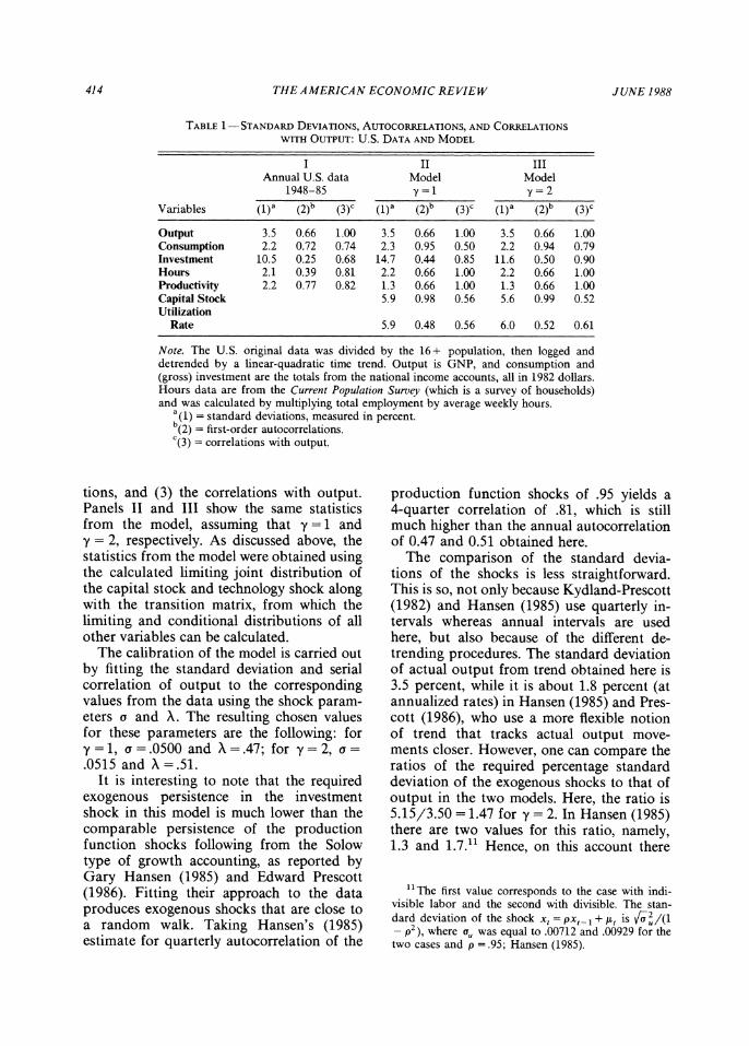
Panel I of Table 1 portrays the statistics calculated with actual data: (1) the standard deviations, (2) the first-order serial correla-


TABLE 1-STANDARD DEVIATIoNs, AUTOCORRELATIONS, AND CORRELATIONS

WITH OUTPUT: U.S. DATA AND MODEL

I II III Annual U.S. data Model Model

1948-85 y=1 y= 2

Variables (1)a (2)b (3)c (1)a (2)b (3)C (1)a (2)b (3)c

Output 3.5 0.66 1.00 3.5 0.66 1.00 3.5 0.66 1.00 Consumption 2.2 0.72 0.74 2.3 0.95 0.50 2.2 0.94 0.79 Investment 10.5 0.25 0.68 14.7 0.44 0.85 11.6 0.50 0.90 Hours 2.1 0.39 0.81 2.2 0.66 1.00 2.2 0.66 1.00 Productivity 2.2 0.77 0.82 1.3 0.66 1.00 1.3 0.66 1.00 Capital Stock 5.9 0.98 0.56 5.6 0.99 0.52 Utilization

Rate 5.9 0.48 0.56 6.0 0.52 0.61

Note. The U.S. original data was divided by the 16 + population, then logged and detrended by a linear-quadratic time trend. Output is GNP, and consumption and (gross) investment are the totals from the national income accounts, all in 1982 dollars. Hours data are from the Current Population Survey (which is a survey of households) and was calculated by multiplying total employment by average weekly hours.

a(1) = standard deviations, measured in percent. b(2) = first-order autocorrelations. C(3) = correlations with output.

tions, and (3) the correlations with output. Panels II and III show the same statistics from the model, assuming that y =1 and y = 2, respectively. As discussed above, the statistics from the model were obtained using the calculated limiting joint distribution of the capital stock and technology shock along with the transition matrix, from which the limiting and conditional distributions of all other variables can be calculated.

The calibration of the model is carried out by fitting the standard deviation and serial correlation of output to the corresponding values from the data using the shock parameters a and X. The resulting chosen values for these parameters are the following: for y=1, a=.0500 and X=.47; for y=2, a= .0515 and X=.51.

It is interesting to note that the required exogenous persistence in the investment shock in this model is much lower than the comparable persistence of the production function shocks following from the Solow type of growth accounting, as reported by Gary Hansen (1985) and Edward Prescott (1986). Fitting their approach to the data produces exogenous shocks that are close to a random walk. Taking Hansen's (1985) estimate for quarterly autocorrelation of the

production function shocks of .95 yields a 4-quarter correlation of .81, which is still much higher than the annual autocorrelation of 0.47 and 0.51 obtained here.

The comparison of the standard deviations of the shocks is less straightforward. This is so, not only because Kydland-Prescott (1982) and Hansen (1985) use quarterly intervals whereas annual intervals are used here, but also because of the different de- trending procedures. The standard deviation of actual output from trend obtained here is 3.5 percent, while it is about 1.8 percent (at annualized rates) in Hansen (1985) and Pres- cott (1986), who use a more flexible notion of trend that tracks actual output movements closer. However, one can compare the ratios of the required percentage standard deviation of the exogenous shocks to that of output in the two models. Here, the ratio is 5.15/3.50 = 1.47 for y = 2. In Hansen (1985) there are two values for this ratio, namely, 1.3 and 1.7.11 Hence, on this account there

"1The first value corresponds to the case with indivisible labor and the second with divisible. The standard deviation of the shock x, = pxt_I + lt is V 2/(1 - p2) where a, was equal to .00712 and .00929 for the two cases and p =.95; Hansen (1985).


seems to be no advantage to the present model.

However, there is indeed an advantage when the meaning of the exogenous shock in this framework and in the Kydland-Prescott, 1982, Hansen 1985 economies are taken into account. In the latter models, the shock affects the productivity of the entire capital stock and labor inputs. In the present model the shock refers only to the productivity of new capital goods. Since productivity changes related to new capital are perhaps more plausible than overall productivity changes, a shock of a given magnitude seems a weaker requirement in this model than in the models where the shock applies to all the existing capital stock and labor.

An inspection of Table 1 will now com- mence. The most salient feature of the standard deviations of the actual data, shown in colunm (1) of panel I, is the well-known fact that investment is much more volatile than output, and consumption is less. In column (1) of panels II and III it can be seen that, in general, the model qualitatively mimics this behavior and quantitatively exaggerates it.

Column (2) of panel I describes the persistence of the movements in the different variables, as characterized by their first-order serial correlations. Consumption and productivity have the highest autocorrelations, and investment the lowest. The model also performs fairly well in this respect. In column (2) of panels II and III consumption has the highest autocorrelation, productivity the second, and investment the lowest.

The actual correlations with output ap- pear in column (3) of panel I. Productivity and hours have the highest correlation with output but the other variables, particularly consumption, are fairly close. This feature is reproduced by the model simply because by construction there is perfect correlation of hours with output.'2 The procycical behavior of consumption, however, is highly de- pendent on the value of y. When y = 1, the correlation of consumption with output is

only .50. For y = 2, this correlation increases to .79, closer to the actual value of 0.74. Also, increasing y from 1 to 2, which corresponds to reducing the amount of intertemporal substitution, lowers the standard deviation of investment from 14.7 to 11.6 percent, much closer to the actual data value of 10.5 percent. Overall, if this exercise is used to choose the risk-aversion parameter y from the values 1 and 2, the best fit would correspond to y = 2.

To check the sensitivity of the results to the labor supply elasticity parameter (chosen to be 1.7), the figures in panels II and III were computed again using alternative values. The resulting moments (not shown) are in general very similar to those shown in Table 1.13

V. Concluding Remarks

This paper addressed the macroeconomic effects of direct shocks to investment in a framework where the utilization rate of in- stalled capital is endogenous. The shocks considered take the form of technological changes that affect the productivity of new capital goods only.

The results in the paper suggest that a variable capacity utilization rate may be important for the understanding of business cycles. It provides a channel through which investment shocks via their impact on capacity utilization can affect labor productivity and hence equilibrium employment. Such a mechanism may allow for a smaller burden to be placed on intertemporal substitution in generating observed patterns of aggregate fluctuations.

Because of the variable capacity utilization the model predicts the Keynesian type result of less than "full-capacity equilibrium." Unlike in the Keynesian model, however, the labor market always clears and partial capacity utilization is socially opti-

12This is a consequence of the log-linear structure of production and depreciation, and the way the only stochastic shock was introduced.

13 There was one expected change though. Holding constant the percentage standard deviation and first- order autocorrelation coefficient of output, the standard deviation of hours increases to 2.3 for 1/0 = 2 and declines to 2.0 for 1/0 = 1.4 (for both values of y).


mal. Ironically, even if the labor market is in continuous equilibrium, it is Keynes' notion of user cost that generates a Keynesian type of expansionary effect of investment shocks on employment.

APPENDIX

Consider a version of the model developed in the text which still incorporates shocks to the marginal efficiency of investment, but where the rate of capacity utilization is held fixed and the utility function U is of the standard general form (i.e., not restricted to U(c,, I) = U(ct - G(l,)). It will now be established that in such a framework consumption covaries negatively with investment and labor supply when shocked by shifts in the marginal efficiency of newly produced capital.

In the setting just described the representative agents' dynamic programming problem is given by

(kt; t) (cmax [U(ct, t)

+ /3 V(kt+l; ?t?+) d4F(ct?iIct)j

subject to

c = F(kt, It)- [kt+I- kt(1- 8)j/(1? E).

The efficiency condition associated with the agent's consumption/leisure decision is

Ul(ct, It)F2(kt, It) = -U2(Ct, lt).

Now suppose in period t that Et rises. By using the above efficiency condition in conjunction with the fact that it = F(kt, It)- ct- two restrictions can be seen to constrain the equilibrium movements of ct, it, and it.

(Al) - [El J - L2/M) + U21] f _ [22 + M12 (-L2 /M1)]U2 F22 IF2}

dc1 dlt x -=

det det

(A2) t dE,

[jU11(-V2AU1) + U21]

{ [i !Li 2/U1) + 2LU12( -C2/ /1) + U22] ]-2 F22/F2 } di

de,

Thus, a shock to the marginal efficiency of newly produced capital which causes current investment to rise will lead to an expansion of current labor effort and a fall in current consumption, provided that consumption and leisure are normal goods, that is, [U22 + E12( - 2/11)] and [Ul( - J2/U1) ? __ 211 <0.

When, as in the text, the utility function is restricted to have the form U(c,, I) = U(ct - G(li)) income effects have no influence on labor supply. Equation (A2) still holds in this case, but dl,/dct = 0 since [U1k(- U2/

1) + ?U211 = 0. Equation (Al) no longer constitutes a restriction across movements in consumption and labor supply, but it is easy to see from the condition ct + i= F(kp, lt) that dct/det = - dit/det. Conse- quently, consumption still moves negatively with investment in response to prospective future production function shocks. A general discussion about the implications of using time-separable preferences in models of business cycles is contained in Barro and King (1984).

REFERENCES

Barro, Robert J. and King, Robert G., " Time- Separable Preferences and Intertemporal Substitution Models of the Business Cy- cle," Quarterly Journal of Economics, Nov- ember 1984, 99, 817-39.

Bertsekas, Dimitri P., Dynamic Programming and Stochastic Control, New York: Aca- demic Press, 1976.

Calvo, Guillermo A., "Efficient and Optimal Utilization of Capital Services," American Economic Review, March 1975, 65,181-86.

Friend, Irwin and Blume, Marshall E., "The De- mand for Risky Assets," American Eco- nomic Review, December 1975, 65, 900-22.

Hansen, Gary D., "Indivisible Labor and the Business Cycle," Journal of Monetary Eco- nomics, November 1985, 16, 309-27.

Hansen, Lars P. and Singleton, Kenneth J., "Sto- chastic Consumption, Risk Aversion, and the Temporal Behavior of Asset Returns," Journal of Political Economy, April 1983, 91, 249-65.

Heckman, James, J. and Macurdy, Thomas, "A Life-Cycle Model of Female Labor Sup-


ply," Review of Economic Studies, January 1980, 47, 47-74. [Corrigendum, October 1982, 47, 659-60.]

Hercowitz, Zvi, "The Real Interest Rate and Aggregate Supply," Journal of Monetary Economics, September 1986, 18, 121-45.

Keynes, John M., The General Theory of Em- ployment, Interest and Money, London: Macmillan, 1936.

Kydland, Finn E. and Prescott, Edward C., "Time-to-Build and Aggregate Fluctua- tions," Econometrica, November 1982, 50, 1345-70.

Long, John B. and Plosser, Charles I., "Real Business Cycles," Journal of Political Econ- omy, February 1983, 91, 39-69.

Lucas, Robert E., "Capacity, Overtime, and Empirical Production Functions," Ameri- can Economic Review, March 1970, 60, 23-27.

., Prescott, Edward C. and Stokey, Nancy L.,, "Recursive Methods for Eco- nomic Dynamics," unpublished manu-

script, Department of Economics, Univer- sity of Minnesota 1985.

Macurdy, Thomas, "An Empirical Model of Labor Supply in a Life-Cycle Setting," Journal of Political Economy, December 1981, 89, 1059-85.

Merrick, John J., "The Anticipated Real In- terest Rate, Capital Utilization and the Cyclical Pattern of Real Wages," Journal of Monetary Economics, January 1984, 13, 17-30.

Prescott, Edward C., "Theory Ahead of Busi- ness-Cycle Measurement" Carnegie-Roch- ester Conference Series on Public Policy, Autumn 1986, 25, 11-44.

Sargent, Thomas J., "Tobin's q and the Rate of Investment in General Equilibrium," Carnegie-Rochester Conference Series on Public Policy, Spring 1980, 12, 107-54.

Taubman, Paul and WiLkinson, Maurice, "User Cost, Capital Utilization and Investment Theory," International Economic Review, June 1970, 11, 209-15.

Documents

Investment, Capacity Utilization, and the Real Business · PDF fileInvestment, Capacity Utilization, and the Real Business Cycle By JEREMY GREENWOOD, Zvi HERCOWITZ, AND GREGORY W