FEDERAL RESERVE BANK OF SAN FRANCISCO

WORKING PAPER SERIES

The views in this paper are solely the responsibility of the authors and should not be interpreted as reflecting the views of the Federal Reserve Bank of San Francisco or the Board of Governors of the Federal Reserve System. This paper was produced under the auspices for the Center for the Study of Innovation and Productivity within the Economic Research Department of the Federal Reserve Bank of San Francisco.

Investment Behavior of U.S. Firms over Heterogeneous Capital Goods: A Snapshot

Daniel J. Wilson

Federal Reserve Bank of San Francisco

March 2006

Working Paper 2004-21 http://www.frbsf.org/publications/economics/papers/2004/wp04-21bk.pdf

Investment Behavior of U.S. Firms over

Heterogeneous Capital Goods: A Snapshot

Daniel Wilson (Federal Reserve Bank of San Francisco)1

Draft: March 2006

1Economist, Federal Reserve Bank of San Francisco, 101 Market St., MS 1130, San Fran-

cisco, CA 94105; (415) 974-3423 (o¢ ce), (415) 974-2168 (fax); Daniel.Wilson@sf.frb.org

(email). Geo¤rey MacDonald provided superb research assistance. This paper bene�tted

from helpful comments from Bob Chirinko, Mark Doms, Bart Hobijn, Kevin Stiroh and sem-

inar participants at the FRBSF and Center for Economic Studies (Census). The research in

this paper was conducted while the author was a research associate at the CES and California

Census Research Data Center (CCRDC); special thanks go to Ritch Milby of the CCRDC.

Research results and conclusions expressed are those of the author and do not necessarily

indicate concurrence by the Bureau of the Census, the CES, or the Federal Reserve System.

This paper has been screened to ensure that no con�dential data are revealed.

Abstract

Recent research has indicated that investment in certain capital types, such as comput-

ers, has fostered accelerated productivity growth and enabled a fundamental reorgani-

zation of the workplace. However, remarkably little is known about the composition

of investment at the micro level. This short paper takes an important �rst step in

�lling this knowledge gap by looking at the newly available micro data from the 1998

Annual Capital Expenditure Survey (ACES), a sample of roughly 30,000 �rms drawn

from the private, nonfarm economy. The paper establishes a number of stylized facts.

Among other things, I �nd that in contrast to aggregate data the typical �rm tends to

concentrate its capital expenditures in a very limited number of capital types, though

which types are chosen varies greatly from �rm to �rm. In addition, computers ac-

count for a signi�cantly larger share of �rms�incremental investment than they do of

lumpy investment. [Keywords: Capital Heterogeneity, Investment; JEL Codes D21,

D24, D29.]

1 Introduction

Very little is known about �rms�disaggregate investment behavior. Economists�priors

regarding the composition of investment at the �rm level have been based primarily on

economy-wide or industry-level capital �ows information. These latter data can say

little about the degree of microeconomic heterogeneity in investment composition. Is

the composition of investment, and thus perhaps the quality of investment and capital,

relatively constant across �rms within an industry or do �rms in the same industry

tend to choose considerably di¤erent types of assets to invest in. Recent research has

shown that the composition of investment can be vital to understanding investment

dynamics over the business cycle (Tevlin and Whelan (2003)) as well as capital�s role

in explaining productivity di¤erences (Caselli and Wilson (2004), Wilson (2004)).

Moreover, priors based on economy-wide or industry-level data may be inac-

curate for a couple of reasons. First, there is no reason to expect the capital �ows

patterns of individual �rms to be similar to those at the aggregate level. This is

particularly true in light of the growing body of evidence regarding heterogeneity at

the micro level in terms of total-factor productivity, employment, and total investment

(Haltiwanger (1997), Davis, et al. (1996), Caballero, et al. (1995)). Numerous studies

have shown that aggregate measures, even up built up from microeconomic data, often

mask important variations in the measures at the micro level. For example, invest-

ment at the aggregate level is fairly smooth over time despite enormous lumpiness at

the micro level (Doms and Dunne (1998), Caballero, et al. (1995)).

The second reason to be skeptical of priors concerning �rm behavior based on

industry-level capital �ows data is that these data, at least in the U.S., are in fact not

currently based on micro source data. The U.S. capital �ows tables, constructed by

the Bureau of Economic Analysis (BEA), are instead primarily based on occupational

employment distributions combined with data on the aggregate supply of asset-speci�c

capital and aggregate investment by industry.1 The basic idea is as follows: when

estimating computer investment by the Finance industry, the BEA starts with total

value of shipments of computers (from the Annual Survey of Manufacturers), subtracts

o¤ estimates of net exports and purchases of computers by consumers and governments

to get domestic supply, and then assigns a fraction of domestic supply to Finance in

1See Becker, Haltiwanger, Jarmin, Klimek, and Wilson (2005) for a discussion of these BEA data

and a comparison to potential alternative capital �ows tables based on the 1998 ACES.

1

proportion to Finance�s share of total computer programmers� employment. This

resulting investment value may be further adjusted to be consistent with source data

on total investment by the Finance industry. Inferring capital �ows from occupational

employment matrices relies on extremely restrictive conditions that are unlikely to hold

in reality. The fact that U.S. capital �ows data may come as a surprise to many readers

since these data are widely used by researchers.

Both of the above problems are due to a previous lack of data on disaggregate

investment at the micro level. This has changed, however, with the full-scale introduc-

tion of asset-type detail in the Census Bureau�s Annual Capital Expenditures Survey

(ACES) in 1998. (This asset-type detail was also collected in the 2003 ACES, which

was not yet available at the time of this writing.). The 1998 ACES is unique as the

only large-scale micro-level U.S. survey of investment that disaggregates investment

into a full range of detailed asset types (i.e., beyond simply total equipment and total

structures, and beyond just one or two asset types such as computers or transportation

equipment). These rich data on disaggregate investment o¤er a point-in-time snapshot

of investment composition choices by a large number of �rms spanning the U.S. private

nonfarm economy.

This short paper uses the 1998 ACES micro data �le to present some of the

�rst evidence on �rm-level, cross-sectional patterns regarding capital mix. First, I �nd

substantial di¤erences in investment composition across �rms, even within narrowly-

de�ned industries. Second, certain capital types (e.g., Computers, Software, Furniture,

General Purpose Machinery)2 are shown to be used across a wide range of industries,

indicating that they are general purpose capital goods. Third, I �nd evidence that cer-

tain types of capital goods tend to be bundled, i.e., purchased in conjunction with each

other. Here, I focus on Computers, given recent work showing computers�importance

for productivity growth (e.g., Wilson (2004); Gilchrist, et al. (2004); Brynjolfsson &

Hitt (2003); Oliner & Sichel (2000)). I �nd that Computers tend to be purchased in

conjunction with Software, Scienti�c Instruments, and Furniture, among other types.

Fourth, it is shown that the typical �rm tends to concentrate its capital expenditures in

a very limited number of capital types. However, which types are chosen varies greatly

from �rm to �rm. Lastly, I �nd that investment that takes place during lumpy invest-

ment episodes, or �spikes�, identi�ed at the �rm level, has a systematically di¤erent

2Throughout the paper, capital type names are capitalized to indicate that they refer to speci�c

categories of capital listed in the Annual Capital Expenditures Survey.

2

composition than that of incremental investment. Speci�cally, Computers account for

a signi�cantly larger share of �rms�incremental investment than of lumpy investment.

These �ndings have important implications in terms of the economic modeling of

production, business cycle dynamics, and optimal public policy. Most economic models

of production or investment assume a single capital stock, or perhaps one for equipment

and one for structures. The �nding in this paper that the composition of capital varies

greatly across �rms strongly suggests that these models may be misspeci�ed, especially

in light of recent research showing that the composition of capital is an important

factor in production.3 As our economic models evolve to incorporate the e¤ects of

capital composition, a solid understanding of the patterns of disaggregate investment

at the micro level will be key. This paper is an important �rst step in providing that

understanding.

In terms of business cycle dynamics, the �nding that the composition (e.g.,

computers�share of investment) of investment during investment spikes is signi�cantly

di¤erent from that of incremental investment, coupled with the previously established

fact that microeconomic spikes comprise a large portion of aggregate investment during

booms, suggests that capital composition and quality may vary importantly over the

business cycle. For instance, if capital quality tends to be higher for incremental

investment, and incremental investment is a lower share of aggregate investment during

booms, then the volatility of quality-adjusted capital over the cycle may be less than

previously thought.

Lastly, the �ndings in this paper may have implications for public policy, partic-

ularly tax policy. For instance, policymakers in the U.S. often enact special accelerated

depreciation allowances for certain capital types (e.g., high-tech equipment) as tem-

porary measures aimed at spurring an economic recovery. Because the composition

of investment varies greatly across �rms and industries, these special allowances will

bene�t certain �rms and industries more so than others. The non-uniform incidence

of these allowances likely is not fully appreciated by policymakers. Furthermore, if

high-tech equipment comprise a larger share of investment during recessions (when

incremental investment is predominant), then targetting this type of equipment with

special allowances may in fact be optimal.

3See, e.g., Cummins & Dey (1998), Jorgenson and Stiroh (2000), Caselli and Wilson (2004), and

Wilson (2004).

3

2 Data

2.1 1998 Annual Capital Expenditures Survey

The principal source of data for this paper is the 1998 Annual Capital Expenditures

Survey (ACES).4 The ACES is conducted annually by the U.S. Census Bureau to elicit

information on capital expenditures by U.S. private, nonfarm companies. The annual

ACES data are used by the BEA in constructing the National Income and Product

Accounts (NIPA).

In typical years, the ACES queries companies on their expenditures on total

equipment and total structures, in addition to related values such as book value of

capital assets, accumulated depreciation, retirements, etc.. In the 1998 survey, how-

ever, the ACES additionally required �rms to report their investment broken down

by 55 separate types of capital �26 types of equipment and 29 types of structures.

These data on disaggregate investment allow one to observe the complete composition

of �rms�investment.

In fact, the survey requests �rms to break out their capital expenditures in this

way separately for each of the industries in which they operate. Except in Section 3.4,

the analyses in this paper are based on the ACES data as aggregated to the �rm-level.

The 1998 ACES sampling frame consists of all U.S. private, nonfarm employers.5

All companies with 500 or more employees were surveyed while smaller employers were

surveyed based on a strati�ed random sampling such that larger �rms were sampled

with a higher probability. Response to the ACES is legally required so response

rates are extremely high. The �nal sample consists of nearly 34,000 �rms, of which

approximately half have 500 or more employees. 27,712 �rms in the sample had non-

zero investment. Except where otherwise noted, all of the analysis in this paper will

be based on this sample of �rms with non-zero investment.

4For more details regarding the 1998 Annual Capital Expenditures Survey, including the published

aggregate data and the actual survey questionaires, see Census Bureau (2000).5In addition, a sample of companies with zero employees were sent an abbreviated questionaire

which did not request the disaggregate investment detail.

4

3 Cross-Sectional Patterns of Firm-Level Investment

Behavior

In this section, I utilize the 1998 ACES microdata to answer the following interesting

and previously unexplored questions related to disaggregate investment behavior:

1. How extensive is investment in speci�c asset types?

2. How intensive is investment in speci�c asset types?

3. What is the range of industries using each asset type?

4. To what extent does investment composition vary across sectors/divisions within

a parent �rm?

5. To what extent are di¤erent asset types purchased in conjunction? Speci�cally,

what asset types tend to be purchased in conjunction with computers?

6. How �lumpy�is investment in the asset-type dimension? I.e., do �rms tend to

invest in a wide range of asset types or just a few?

7. Is the composition of investment di¤erent during investment spikes than during

periods of incremental investment?

3.1 The Extensive Margin of Asset-Speci�c Investment

Whether or not a �rm decides to invest in a particular capital good can be thought of

as the extensive margin of the investment decision. (The intensive margin, how much

of the capital good to actually purchase or lease, is analyzed in the next subsection).

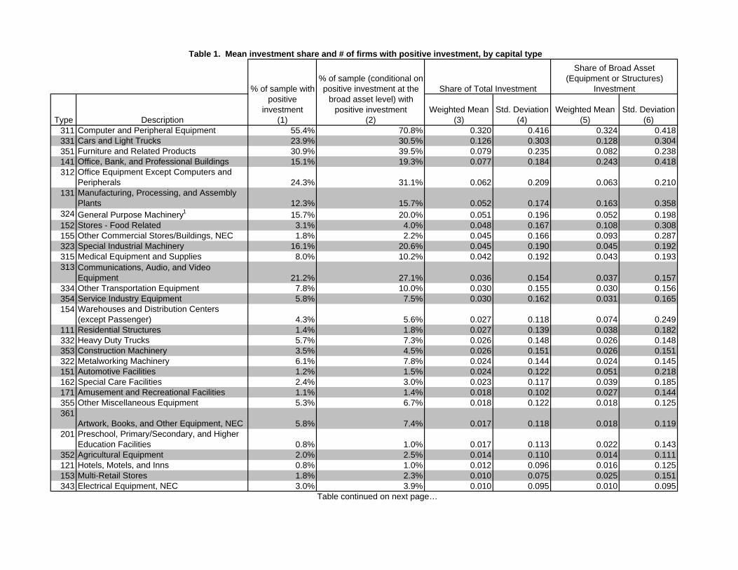
Columns (1) and (2) of Table 1 give the proportion of sample �rms that report pur-

chasing each type of capital. Column (2) gives the unconditional proportion; Column

(2) gives the proportion conditional on �rms having non-zero investment in the capital

type�s broad asset class (equipment or structures).

Computers are the most common type of investment, with over 55% of �rms

purchasing at least some computers or computer peripheral equipment. This share

jumps to 71% if one excludes �rms that have no equipment investment at all. At

�rst blush, it would appear that the propensity to invest in Computers is higher for

manufacturing �rms: 59% compared to 54.5% for non-manufacturing (not shown).5

However, this di¤erence is primarily because non-manufacturers are simply less likely

to invest in equipment at all (75% of non-manufacturing �rms had positive equipment

investment compared to 90% of manufacturing �rms). Among equipment-buying

�rms, 72% of non-manufacturers invested in Computers while 66% of manufacturers

did so.

It is interesting to compare these numbers on computer investment to analogous

statistics reported by Dunne, Foster, Haltiwanger, and Troske (2002). Dunne, et al.

�nd that the proportion of manufacturing plants in the Annual Survey of Manufacturers

(ASM) reporting positive computer investment rose from about 10% in 1977 to just

over 60% by 1992. Again, I �nd the proportion among manufacturing �rms in 1998

to be 59%. The Dunne, et al. numbers are likely overestimated, however, since about

40% of sampled ASM plants did not respond to the computer question in the ASM

survey. Non-respondents are arguably far more likely to have zero computer investment

than the respondents. Thus, the upward trend in the proportion of �rms (or plants)

investing in computers likely continued between 1992 and 1998.

After computers, the next most common types of investment are Furniture

(31%), O¢ ce Equipment (24%), Autos (24%), Communications Equipment (21%),

Special Industry Machinery (16%), General Purpose Machinery (16%), O¢ ce Build-

ings (15%), Software (14%), and Manufacturing Plants (12%). All other types were

purchased by less than 10% of the sample.

What is striking about these results is that, with the exception of computers, all

other capital types have frequencies will below 50%. In other words, for any particular

non-computer asset type, a randomly-selected �rm is more likely than not to have zero

investment. The surprising infrequency of investment in non-computer asset types

suggests that these asset types either have large non-convex adjustment costs or that

they are characterized by substantial indivisibilities.

3.2 The Intensive Margin of Asset-Speci�c Investment

In this subsection, I characterize the intensive margin of asset-speci�c investment by

computing each asset types average share of total �rm investment. Columns (3) and (5)

of Table 1 show the cross-�rm, weighted-average of each asset type�s share of �rm total

investment (standard deviations are shown in Columns (4) and (6)). Observations are

weighted by sample weight (inverse of sampling probability, adjusted for nonresponses)

which is necessary given the strati�cation of the ACES sampling design. Column (3)6

gives the asset type�s average share of �rms�total investment while Column (5) gives the

asset type�s average share of its broad asset class (total equipment or total structures).

The asset types in the table are sorted by average share of total investment.

Computers are nearly one-third of total (and equipment) investment for the

average �rm, a much higher share than that of any other capital good. Hence, not only

are Computers the most common type of investment as discussed above, they are also

the largest share of investment on average. The next largest type of investment tends to

be Autos, which, on average, comprise about one-eighth of �rm total (and equipment)

investment. Interestingly, the fact that Computers are a much larger average share of

investment than Autos is in sharp contrast to the picture one gets from the aggregate

data. According to the published aggregate ACES data (and similarly for BEA capital

�ows data), Autos actually comprised a larger share of economy-wide investment in

1998 than did Computers: 17% of equipment compared to 14% for Computers. This

contrast between the aggregate and �rm level shares reveals that �rms that are large

(in terms of total investment) tend to invest more intensively in autos than computers,

while the opposite is true for small �rms.

Other capital goods that make up at least 5% of the average �rm�s total invest-

ment are Furniture (7.9%); O¢ ce Buildings (7.7%); Other O¢ ce Equipment (6.2%);

Plants (5.2%); and General Purpose Machinery (5.0%).

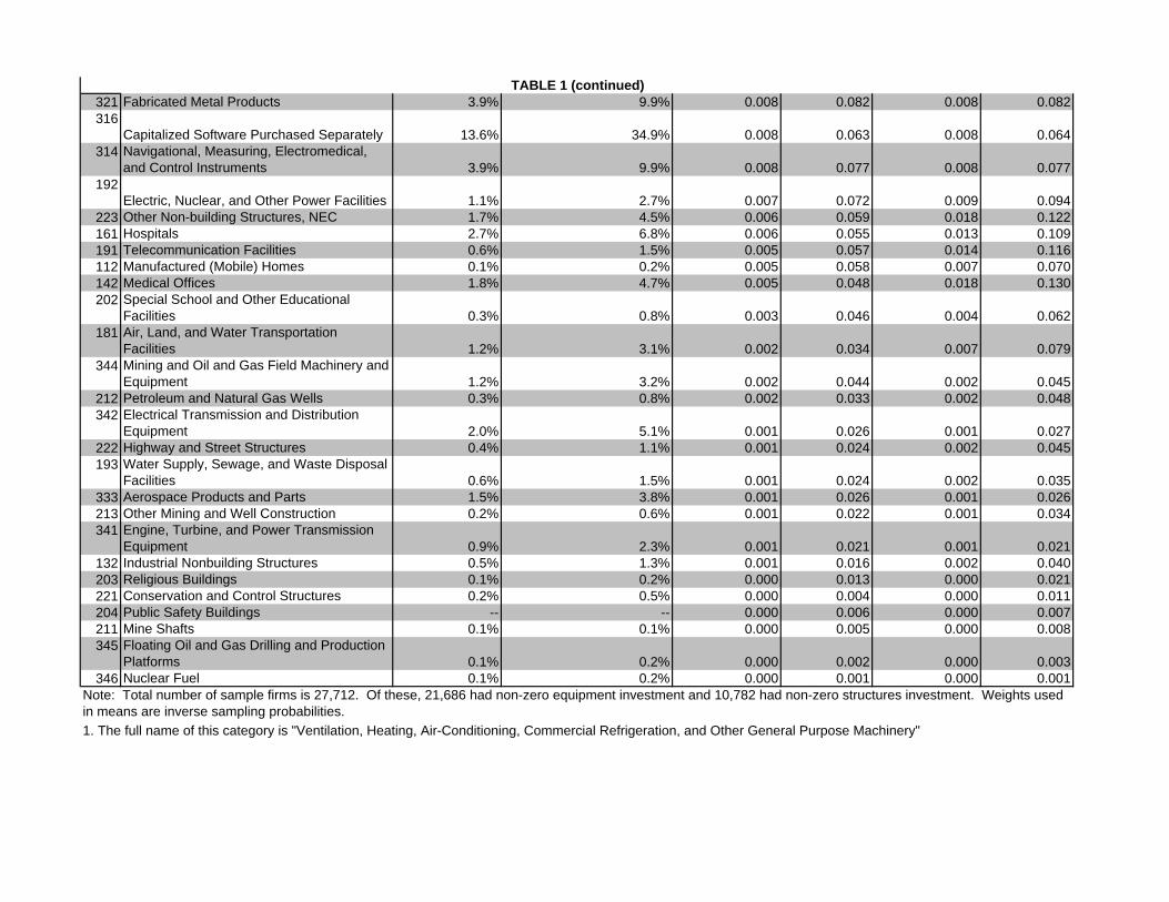
It should be noted that a small average investment share could arise either from

a large number of �rms having a small investment share or from a small number of �rms

having a large investment share (while the rest of �rms are near zero). The latter tends

to be the case for structures while the former tends to the case for equipment types.

For example, �Other Commercial Stores/Buildings, NEC�averages a relatively high

4.5% of total investment (9th most out of the 55 types) even though less than 2% of the

sample invested in this type of structure. In contrast, 13.6% of the sample purchased

software but software accounted for less than 1% of the average �rm�s investment.

Part of the reason for the high frequency of software investment coupled with

its low average share �lower than software�s aggregate investment share in the NIPAs

� is that the ACES software category is narrower than that of the NIPAs. In the

ACES, �rms are instructed to report investment in software �only if capitalized as

part of a tangible asset� and to exclude it �if the purchase is considered intangible

(e.g., licensing agreement) or if expensed such as o¢ ce supplies.�The NIPAs, on the

other hand, classify all software expenditures as investment regardless of whether the

7

�rm accounts for the expenditures as capital or intermediate expenses. (Note that

software that is bundled with, or embedded in, hardware is not counted as software

investment in either ACES or NIPAs.) The fact that Capitalized Software Purchased

Separately, on average, comprises a very small share of �rms�investment even though

a considerable percentage of �rms purchase it may be partially because �rms purchase

this kind of software in conjunction with other kinds of software (including expensed

software). Hence, the average investment share for Capitalized Software Purchased

Separately is likely well below the average share for total software, while the measured

percentage of �rms investing in this kind of software is probably near that for total

software.

3.3 Range of Industries Investing in Each Asset Type

The third interesting question that can be answered with these data is: how broadly is

each capital good used (or at least purchased)? The pervasiveness of investment in an

asset type across a wide range of industries has been cited as a de�ning characteristic of

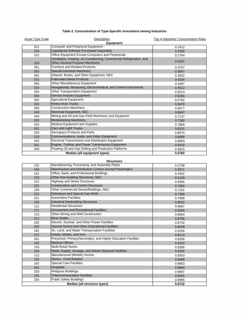
a general purpose technology (Bresnahan and Trajtenberg (1996)). A simple statistic

that the range of use across industries is the investment concentration ratio by the top

four investing industries (at the 3-digit SIC level). Speci�cally, I compute the fraction

of economy-wide investment in a given capital type that is accounted for by the four

industries with the highest levels of investment in that type. A low value for this

�top-4 concentration ratio�indicates that the capital good is used across a wide range

of industries.

Table 2 gives the top-4 concentration ratio for each capital type. The types

of equipment found to have the widest range of use are generally those one would

intuitively expect to be general purpose: Computers, Other O¢ ce Equipment, Soft-

ware, Fabricated Metal Products, General Purpose Machinery, Autos, and Furniture.

Perhaps less intuitive, I also �nd Metalworking Machinery and Medical Equipment to

have widespread use. Interestingly, Communications Equipment does not appear to

be used broadly across industries �its top-4 concentration ratio is 87%. Structures,

as one might expect, generally have much higher concentration ratios then equipment,

re�ecting the more specialized functions that structures have. An exception is Man-

ufacturing, Processing, and Assembly Plants, which tend to be purchased by �rms in

many di¤erent industries.

These results con�rm the common perception that computers and software are8

general purpose capital goods, while they refute the perception that communications

equipment are as well. It should be noted that this is not the �rst paper to report

evidence computers and software are general purpose technologies. Cummins and

Violante (2002), Jovanovic and Rousseau (2005), and others have shown the wide

range of use of these technologies across industries. Their evidence, however, is based

on the BEA capital �ows data, which, as mentioned in Section 1, are not based on

micro source data.

3.4 Analysis of Cross-Sectional Variance

The results in this and previous studies strongly suggest that investment is heteroge-

neous at the micro level. For instance, above we established that the composition of

investment (measured by assets�shares of �rm total investment) varies greatly across

�rms, even within 3-digit industries. Thus, a natural question is whether investment

composition also varies greatly across industry divisions within a �rm. That is, how

much of the variation in an asset type�s share of investment is due to di¤erences across

divisions within a �rm as opposed to di¤erences across �rms? As mentioned in Section

2, the ACES data is actually collected at the level of industry divisions within the �rm,

so it is possible to to answer this question. To do so, I perform a variance decompo-

sition on each asset type�s share of �rm-division level investment into its within- and

between-�rm components. I perform this decomposition both unconditionally and

conditioning on �rms having multiple divisions.

The results show, �rst, that very little of the total �rm-division level variance

in a capital type�s investment share (for any capital type) is within-�rm. Conditional

on �rms having multiple divisions, the ratio of within-�rm to total variance ranges

across asset types from 0.01 to 0.39. For equipment, the median (and mean) ratio

is 0.27; for structures, the median ratio is 0.26 (mean is 0.22). The unconditional

ratios are much lower (median is 0.12 for equipment and 0.13 for structures). Thus,

a substantial majority of the variance in investment shares is between-�rm, suggesting

that establishments/divisions within �rms tend to be fairly homogenous in terms of

their capital composition.

9

3.5 Bundling of investment: The Case of Computers

Capital goods are not used in isolation. They typically are used together as part of

a system of capital infrastructure. This should be especially true for general purpose

capital goods such as computers. Table 3 provides evidence of what capital types

tend to be purchased in conjunction with, or instead of, computers. Speci�cally, for

each capital type, I calculate the partial correlation between the computer investment

share and that type�s investment share, controlling for 3-digit industry e¤ects. Table

3 provides the weighted correlations for those types that have a statistically signi�-

cant partial correlation with computers. Observations are weighted by sample weight

(unweighted correlations, not shown, are very similar).

Among equipment, Computers tend to be purchased in conjunction with Other

O¢ ce Equipment; Scienti�c Instruments; Software; Aerospace Products; Furniture;

and Artwork, Books, & Other Equipment, NEC. Capital goods that generally are

purchased separately from Computers are Communications Equipment; Metalworking

Machinery; Special Industry Machinery; Cars and Light Trucks; Heavy-Duty Trucks;

Engine, Turbine, and Power Transmission Equipment; Electrical and Distribution

Equipment; Mining and Oil & Gas Field Machinery; and Miscellaneous Equipment.

The negative correlation with Communications Equipment is surprising and counter-

intuitive. This result may re�ect that communications equipment typically is embed-

ded in business computer equipment (and hence is recorded as computer investment)

and therefore separate investment in communications equipment is unnecessary.

Among structures, Computers are most often purchased with O¢ ce, Bank, &

Professional Buildings; Multi-Retail Stores; and Other Commercial Buildings/Stores,

NEC. On the other hand, �rms with capital expenditures on the following types of

structures tend not to purchase Computers in the same year: Industrial Nonbuild-

ing Structures; Automotive Facilities; Air, Land, & Water Transportation Facilities;

Telecommunications Facilities; Electric, Nuclear, & Other Power Facilities; Petroleum

& Natural Gas Wells; and Other Mining & Well Construction.

3.6 Investment Variety

It is well documented that investment is extremely lumpy over time at the microeco-

nomic level (see, e.g., Doms and Dunne (1998) and Power (1999)). However, we know

little about the microeconomic �lumpiness,�or concentration, of investment over cap-

10

ital types. The question is: in a given year, do �rms tend to invest only in a small

number of capital types or do they spread their investment dollars across a wide variety

of types?

To answer this question, for each �rm I calculated the number of asset types in

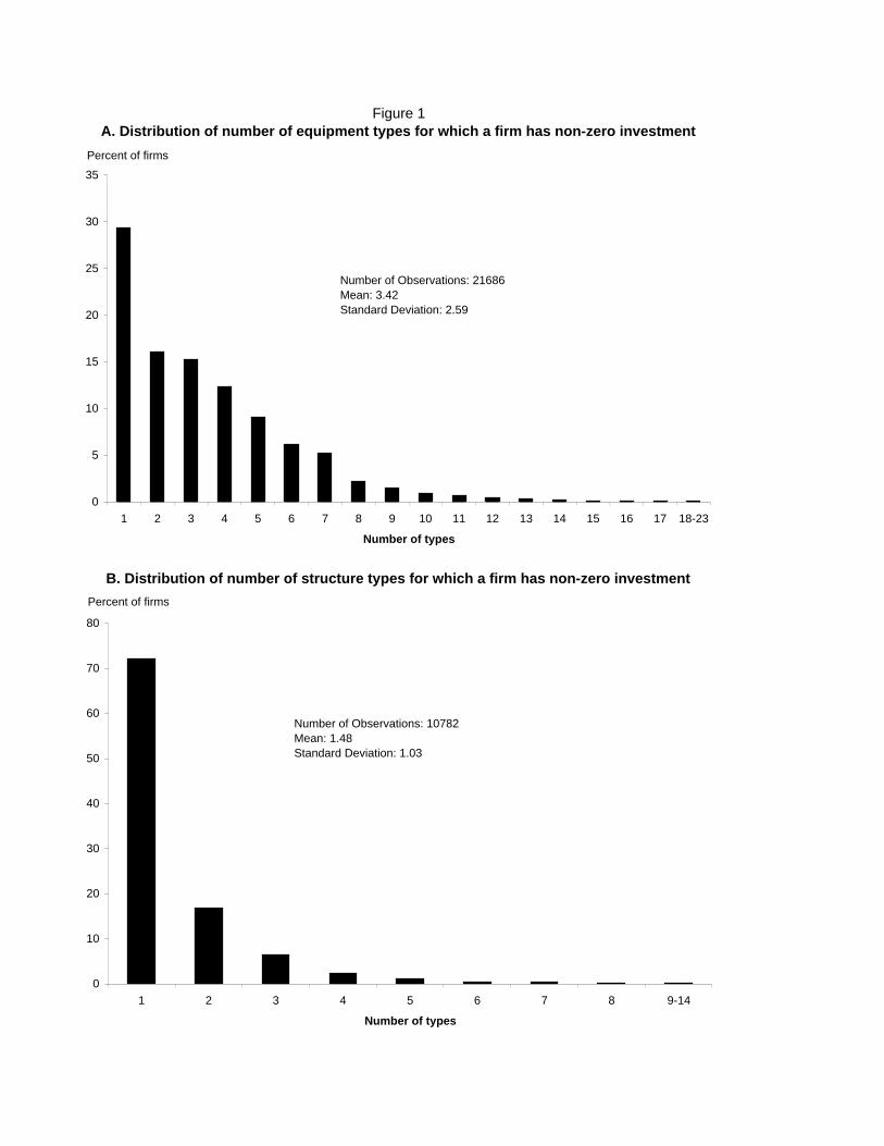
which the �rm reported positive investment. Figures 1a and 1b show the cross-sectional

distribution of this number across the �rms in our sample. Figure 1a gives the distri-

bution for equipment; Figure 1b gives the distribution for structures. Of the 21,686

�rms that reported positive equipment investment, a little less than 30% of investing

�rms reportedly purchased only one type of equipment. 16% reported investment in

two types, 15% in three types, 12% in four types, and 9% in �ve types. The frequencies

decline with the number of reported types (though, for non-disclosure purposes, the tail

of the distribution is truncated at 18-23 types). The average equipment-purchasing

�rm reported investment in 3.4 types of equipment.

As expected, investment in structures tends to be highly concentrated. In fact,

72% of the 10,782 �rms that reported positive structures investment invested in just one

type of structure. 16% reported investing in two types, almost 7% reported investing

in three types, and the frequencies continue to decline thereafter with the number of

types. The average number of structure types that �rms invested in (conditional on

having positive structures investment) was 1.5.

An alternative way to assess how concentrated or diversi�ed �rm level invest-

ment is is to compute the proportion of the sample that invested in three (e.g.) or

more capital types (within the broad asset class, equipment or structures). I call

this statistic the 3+ equipment (structures) share. For the entire sample (of 27,712

�rms), the 3+ equipment share is 42.8% and the 3+ structures share is 4.3%. For the

subsample of �rms with non-zero equipment investment, the 3+ equipment share is

54.7%; for the subsample of structures-buying �rms, the 3+ structures share is 11.1%.

The variety of �rms�investments does of course vary by �rm size. Table 4 shows,

separately for equipment and structures, the mean number of types in which �rms

invest and the 3+ share. For both equipment and structures, I �nd that larger �rms

tend to invest in a larger variety of capital goods. This is not surprising considering

that larger �rms tend to be more diversi�ed in terms of their business operations and

hence more diversi�ed in terms of their physical capital needs.6

6As discussed below, there is the possibility that �rms with positive but near-zero investment in a

type report that investment as zero. This may be more problematic for smaller �rms since they are

11

I also brie�y note here that investment variety also varies noticeably by industry.

It appears that quasi-public industries, such as educational services, utilities, pipelines,

and water services, and �nance industries tend to report investment in the most number

of types.

The low number of types that most �rms report investing in, especially for

structures, in part may re�ect inaccuracy on the part of respondents. That is, de-

composing their �rm�s capital expenditures into a large number of disaggregate asset

types may impose an exorbitant time and record-keeping burden on respondents. It is

di¢ cult to determine with certainty whether respondents truncate the number of asset

types for which they report investment, but it may contribute to measurement error

in the investment shares.

Nonetheless, the fact that 72% of �rms report investment in only a single struc-

ture type, combined with the fact (established in Table 1) that no single structure type

comprises more than a quarter of the average �rm�s investment in structures, suggests

that �rms tend to concentrate construction investment on a single type of structure

but that this type di¤ers from �rm to �rm.7 The particular type of investment a �rm

chooses appears to be primarily determined by the industry to which the �rm belongs,

as evidenced by the high concentration ratios in Table 2.

3.7 The Composition of Spikes versus Incremental Investment

As mentioned above, it is well known that much investment at the micro level takes

place in spikes rather than smooth incremental investment. A number of macroeco-

nomic models build on this micro evidence to explain aggregate investment dynamics

[e.g., Caballero and Engels (1999)]. It generally is assumed that the investment oc-

curing in spikes and the investment occuring in increments are of the same qualitative

nature. In particular, it is assumed that there is no di¤erence in quality, i.e., the

more likely to have near-zero investment and also to have less-developed accounting systems. Thus,

part of the correlation between �rm size and reported investment variety may be due to misreporting.7This �nding is consistent with the theoretical model of optimal adoption of complementary capital

goods by Jovanovic and Stolyarov (2000). They show that given �xed costs of investment, the �rm

may invest in complementary capital goods asynchronously rather than simultaneously. Thus, the

�nding that �rms tend to concentrate their structures investment, which should involve higher �xed

costs than equipment investment, on a single type but that this type di¤ers across �rms is consistent

with their theory. A test of this theory would require a time dimension to these data: a �nding that

the concentrated type di¤ers across time within �rms would support the theory.

12

capital-embodied technology, between lumpy and incremental investment. If there is

a di¤erence, however, the true (i.e., quality-adjusted) lumpiness of investment could in

fact be much di¤erent than is currently assumed.

To assess whether the quality composition of investment spikes is fundamentally

di¤erent from that of incremental investment, I start with the �rm-level investment

share for each asset type. I then split the sample into �rms that engaged in an

investment spike (in terms of total investment) in 1998 and those that did not. Lastly,

I compute the weighted-average investment share by type for each subsample (weighting

each �rm by its total investment) and perform a two-sample equality-of-the-means t-

test.

The most common de�nition of an investment spike used in the literature [e.g.,

Doms and Dunne (1998) and Powers (1999)], and thus the de�nition I use, is the

following:

Spikeit = 1 if Iit=Ki;t�1 > 0:20;

Spikeit = 0 otherwise,

where i indexes �rms, Iit denotes total investment, and Ki;t�1 denotes total beginning-

of-year book value of capital.8

For most types, the mean investment share does not di¤er importantly between

the two samples. A notable exception, however, is Computer investment: Computers

comprise 14% of incremental investment, on average, whereas Computers comprise just

12% of investment spikes. This di¤erence is statistically signi�cant at below the 1%

level. Note this result is robust to controlling for 3-digit SIC industry (by demeaning

investment shares by industry mean prior to computing the group means).

That computers represent a larger share of investment in periods of incremen-

tal investment could be because �rms are locked into particular production processes

that require a stable level of computer capital stock, making computer investment less

cyclical than other types of capital. Regardless of the explanation, the result has

at least two important implications. At the aggregate level, given that investment

spikes are far more common during business cycle booms than during troughs, this

result suggests that computers� share of the aggregate capital stock is countercycli-

cal. Computers�share of capital has been shown to be important for understanding

8For the sample used in this paper, t is of course 1998. Note that though the data are for 1998

only, Ki;t�1 = Ki;1997 is observed since beginning-of-year book value of capital is reported.

13

aggregate investment behavior since computer investment may be more sensitive to

the user cost of capital (see Tevlin and Whelan (2003)). Another implication is that,

given computer investment likely embodies more technology per dollar than other types

of investment (see Wilson (2004) for evidence of this), investment in constant-quality

units may actually be less lumpy at the micro level than previously thought.

4 Conclusion

The preceding section began by posing seven previously unanswered questions regard-

ing micro-level investment behavior across heterogeneous asset types. Here I summa-

rize what we have learned here from the 1998 ACES microdata.

1. How extensive is investment in speci�c asset types?

The data show that only investment in computers could be reasonably be char-

acterized as extensive or common. For all other capital types, investment is in

fact a rare phenomenon, with far less than half of �rms investing in a given year

(to the extent that 1998 is a representative year).

2. How intensive is investment in speci�c asset types?

Computers also are found to be the most intensively-purchased capital good, ac-

counting for about one-third of �rm investment for the average �rm. Investment

intensity is much less for all other types, though Autos, Furniture (7.9%), O¢ ce

Buildings (7.7%), Other O¢ ce Equipment (6.2%), Plants (5.2%), and General

Purpose Machinery (5.0%) on average account for at least �ve percent of �rm

investment.

3. What is the range of industries using each asset type?

The asset types that tend to be used by a wide range of industries are: Com-

puters, Other O¢ ce Equipment, Software, Fabricated Metal Products, General

Purpose Machinery, Autos, Furniture, and, surprisingly, Metalworking Machin-

ery and Medical Equipment. Types of structures, on the other hand, tend to be

rather industry-speci�c.

4. To what extent does investment composition vary across sectors/divisions within

a parent �rm?

14

Interestingly, compared with cross-�rm variation, the composition of investment

across asset types varies very little across industry divisions within a �rm. This

�nding suggests that the vast majority of the variation across individual estab-

lishments in terms of investment and capital composition likely is between �rms

and not within �rms. This in turn suggests that �rm-level data should su¢ ce

for analyses related to investment quality/composition.

5. To what extent are di¤erent asset types purchased in conjunction? Speci�cally,

what asset types tend to be purchased in conjunction with computers?

Computers often are purchased in conjunction with Other O¢ ce Equipment;

Scienti�c Instruments; Software; Aerospace Products; Furniture; and Artwork,

Books, & Other Equipment, NEC, while the following goods tend not to be pur-

chased separately: Metalworking Machinery; Special Industry Machinery; Cars

and Light Trucks; Heavy-Duty Trucks; Engine, Turbine, and Power Transmis-

sion Equipment; Electrical and Distribution Equipment; Mining and Oil & Gas

Field Machinery; Miscellaneous Equipment; and, surprisingly, Communications

Equipment.

6. How �lumpy�is investment in the asset-type dimension? I.e., do �rms tend to

invest in a wide range of asset types or just a few?

Investment is remarkably lumpy in the asset dimension, with over half of the

�rms in the ACES sample purchasing fewer than three types of equipment and

nearly 90% of �rms purchasing fewer than three types of structures.

7. Is the composition of investment di¤erent during investment spikes than during

periods of incremental investment?

The data show that, for most capital goods, �rm investment occuring during

lumpy investment episodes, or �spikes,� represents a similar share of total in-

vestment as it does during periods of incremental �rm investment. Computers,

however, are found to account for a signi�cantly larger share of �rm invesment

during incremental-investment periods than during spikes.

These results are just a �rst step in understanding the heterogeneity of invest-

ment across asset types at the �rm level. An important next step should be exploring

the dynamics of asset-speci�c investment. Fortunately, such research should be possi-

ble in the near future as additional surveys similar to 1998 ACES are conducted.15

5 References

References

[1] Abowd, John M., John Haltiwanger, Ron Jarmin, Julia Lane, Paul Lengermann,

Kristin McCue, Kevin McKinney, and Kristin Sandusky. "The Relation Among

Human Capital, Productivity and Market Value: Building Up From Micro Evi-

dence ." Measuring Capital in the New Economy, Editors Carol Corrado, John C.

Haltiwanger, and Daniel E. Sichel. Chicago: University of Chicago Press, forth-

coming.

[2] Bresnahan, T. F., and M. Trajtenberg (1996), �General purpose technologies:

�engines of growth�?�, Journal of Econometrics, Annals of Econometrics 65: 83-

108.

[3] Brynjolfsson, Erik, and Lorin M. Hitt. "Computing Productivity: Firm-Level Ev-

idence." Review of Economics and Statistics 85, no. 4 (2003): 793-808.

[4] Caballero, Ricardo J., and Eduardo M.R.A. Engel. �Explaining Investment Dy-

namics in U.S. Manufacturing: A Generalized (S,s) Approach.�Econometrica 67,

no. 4 (1999): 783-826.

[5] Caballero, Ricardo J., John C. Haltiwanger, and Eduardo M.R.A. Engel. "Aggre-

gate Employment Dynamics: Building From Microeconomic Evidence." American

Economic Review 87, no. 1 (1997): 115-37.

[6] Caballero, Ricardo J., John C. Haltiwanger, and Eduardo M.R.A. Engel. "Plant-

Level Adjustment and Aggregate Investment Dynamics." Brookings Papers on

Economic Activity 0, no. 2 (1995): 1-39.

[7] Caselli, Francesco, and Daniel J. Wilson. "Importing Technology." Journal of Mon-

etary Economics 51, no. 1 (2004): 1-32.

[8] Cummins, Jason G., and Giovanni L. Violante. �Investment-Speci�c Technical

Change in the United States (1947-2000): Measurement and Macroeconomic

Consequences.� Review of Economic Dynamics 5: 243-84.

[9] Davis, Steven J., John C. Haltiwanger, and Scott Schuh. Job Creation and De-

struction. Cambridge, MA: MIT Press, 1996.16

[10] Doms, Mark E., and Timothy Dunne. "Capital Adjustment Patterns in Manufac-

turing Plants." Review of Economic Dynamics 1, no. 2 (1998): 409-29.

[11] Dunne, Timothy, Lucia Foster, John C. Haltiwanger, and Kenneth Troske. "Wage

and Productivity Dispersion in U.S. Manufacturing: The Role of Computer In-

vestment." Journal of Labor Economics 22, no. 2 (2004): 397-429.

[12] Gilchrist, Simon, Vijay Gurbaxani, and Robert Town. "Productivity and the PC

Revolution." Mimeo (2003).

[13] Haltiwanger, John C. "Measuring and Analyzing Aggregate Fluctuations: The

Importance of Building From Microeconomic Evidence." Federal Reserve Bank of

St. Louis Review 79, no. 3 (1997): 55-77.

[14] Jorgenson, Dale W., and Kevin J. Stiroh. "Raising the Speed Limit: U.S. Eco-

nomic Growth in the Information Age." Brookings Papers on Economic Activity,

no. 1 (2000): 125-212.

[15] Jovanovic, Boyan, and Peter Rousseau. �General Purpose Technologies.� NBER

Working Paper 11093 (2005).

[16] Jovanovic, Boyan, and Dmitriy Stolyarov. "Optimal Adoption of Complementary

Technologies." American Economic Review 90, no. 1 (2000): 15-29.

[17] Oliner, Stephen D., and Daniel E. Sichel. "The Resurgence of Growth in the Late

1990s: Is Information Technology the Story?" Journal of Economic Perspectives

14, no. 4 (2000): 3-22.

[18] Power, Laura. "The Missing Link: Technology, Investment, and Productivity."

Review of Economics and Statistics 80, no. 2 (1998): 300-313.

[19] Wilson, Daniel J. "IT and Beyond: The Contribution of Heterogeneous Capital

to Productivity." Federal Reserve Bank of San Francisco Working Paper 2004-13

(2004).

17

A. Distribution of number of equipment types for which a firm has non-zero investment

B. Distribution of number of structure types for which a firm has non-zero investment

Figure 1

0

5

10

15

20

25

30

35

1 2 3 4 5 6 7 8 9 10 11 12 13 14 15 16 17 18-23

Number of types

Percent of firms

Number of Observations: 21686Mean: 3.42Standard Deviation: 2.59

0

10

20

30

40

50

60

70

80

1 2 3 4 5 6 7 8 9-14

Number of types

Percent of firms

Number of Observations: 10782Mean: 1.48Standard Deviation: 1.03

Weighted Mean Std. Deviation Weighted Mean Std. DeviationType Description (1) (2) (3) (4) (5) (6)

311 Computer and Peripheral Equipment 55.4% 70.8% 0.320 0.416 0.324 0.418331 Cars and Light Trucks 23.9% 30.5% 0.126 0.303 0.128 0.304351 Furniture and Related Products 30.9% 39.5% 0.079 0.235 0.082 0.238141 Office, Bank, and Professional Buildings 15.1% 19.3% 0.077 0.184 0.243 0.418312 Office Equipment Except Computers and

Peripherals 24.3% 31.1% 0.062 0.209 0.063 0.210131 Manufacturing, Processing, and Assembly

Plants 12.3% 15.7% 0.052 0.174 0.163 0.358324 General Purpose Machinery1 15.7% 20.0% 0.051 0.196 0.052 0.198152 Stores - Food Related 3.1% 4.0% 0.048 0.167 0.108 0.308155 Other Commercial Stores/Buildings, NEC 1.8% 2.2% 0.045 0.166 0.093 0.287323 Special Industrial Machinery 16.1% 20.6% 0.045 0.190 0.045 0.192315 Medical Equipment and Supplies 8.0% 10.2% 0.042 0.192 0.043 0.193313 Communications, Audio, and Video

Equipment 21.2% 27.1% 0.036 0.154 0.037 0.157334 Other Transportation Equipment 7.8% 10.0% 0.030 0.155 0.030 0.156354 Service Industry Equipment 5.8% 7.5% 0.030 0.162 0.031 0.165154 Warehouses and Distribution Centers

(except Passenger) 4.3% 5.6% 0.027 0.118 0.074 0.249111 Residential Structures 1.4% 1.8% 0.027 0.139 0.038 0.182332 Heavy Duty Trucks 5.7% 7.3% 0.026 0.148 0.026 0.148353 Construction Machinery 3.5% 4.5% 0.026 0.151 0.026 0.151322 Metalworking Machinery 6.1% 7.8% 0.024 0.144 0.024 0.145151 Automotive Facilities 1.2% 1.5% 0.024 0.122 0.051 0.218162 Special Care Facilities 2.4% 3.0% 0.023 0.117 0.039 0.185171 Amusement and Recreational Facilities 1.1% 1.4% 0.018 0.102 0.027 0.144355 Other Miscellaneous Equipment 5.3% 6.7% 0.018 0.122 0.018 0.125361

Artwork, Books, and Other Equipment, NEC 5.8% 7.4% 0.017 0.118 0.018 0.119201 Preschool, Primary/Secondary, and Higher

Education Facilities 0.8% 1.0% 0.017 0.113 0.022 0.143352 Agricultural Equipment 2.0% 2.5% 0.014 0.110 0.014 0.111121 Hotels, Motels, and Inns 0.8% 1.0% 0.012 0.096 0.016 0.125153 Multi-Retail Stores 1.8% 2.3% 0.010 0.075 0.025 0.151343 Electrical Equipment, NEC 3.0% 3.9% 0.010 0.095 0.010 0.095

Table 1. Mean investment share and # of firms with positive investment, by capital type

% of sample with positive

investment

% of sample (conditional on positive investment at the

broad asset level) with positive investment

Share of Total Investment

Share of Broad Asset (Equipment or Structures)

Investment

Table continued on next page…

321 Fabricated Metal Products 3.9% 9.9% 0.008 0.082 0.008 0.082316

Capitalized Software Purchased Separately 13.6% 34.9% 0.008 0.063 0.008 0.064314 Navigational, Measuring, Electromedical,

and Control Instruments 3.9% 9.9% 0.008 0.077 0.008 0.077192

Electric, Nuclear, and Other Power Facilities 1.1% 2.7% 0.007 0.072 0.009 0.094223 Other Non-building Structures, NEC 1.7% 4.5% 0.006 0.059 0.018 0.122161 Hospitals 2.7% 6.8% 0.006 0.055 0.013 0.109191 Telecommunication Facilities 0.6% 1.5% 0.005 0.057 0.014 0.116112 Manufactured (Mobile) Homes 0.1% 0.2% 0.005 0.058 0.007 0.070142 Medical Offices 1.8% 4.7% 0.005 0.048 0.018 0.130202 Special School and Other Educational

Facilities 0.3% 0.8% 0.003 0.046 0.004 0.062181 Air, Land, and Water Transportation

Facilities 1.2% 3.1% 0.002 0.034 0.007 0.079344 Mining and Oil and Gas Field Machinery and

Equipment 1.2% 3.2% 0.002 0.044 0.002 0.045212 Petroleum and Natural Gas Wells 0.3% 0.8% 0.002 0.033 0.002 0.048342 Electrical Transmission and Distribution

Equipment 2.0% 5.1% 0.001 0.026 0.001 0.027222 Highway and Street Structures 0.4% 1.1% 0.001 0.024 0.002 0.045193 Water Supply, Sewage, and Waste Disposal

Facilities 0.6% 1.5% 0.001 0.024 0.002 0.035333 Aerospace Products and Parts 1.5% 3.8% 0.001 0.026 0.001 0.026213 Other Mining and Well Construction 0.2% 0.6% 0.001 0.022 0.001 0.034341 Engine, Turbine, and Power Transmission

Equipment 0.9% 2.3% 0.001 0.021 0.001 0.021132 Industrial Nonbuilding Structures 0.5% 1.3% 0.001 0.016 0.002 0.040203 Religious Buildings 0.1% 0.2% 0.000 0.013 0.000 0.021221 Conservation and Control Structures 0.2% 0.5% 0.000 0.004 0.000 0.011204 Public Safety Buildings -- -- 0.000 0.006 0.000 0.007211 Mine Shafts 0.1% 0.1% 0.000 0.005 0.000 0.008345 Floating Oil and Gas Drilling and Production

Platforms 0.1% 0.2% 0.000 0.002 0.000 0.003346 Nuclear Fuel 0.1% 0.2% 0.000 0.001 0.000 0.001

1. The full name of this category is "Ventilation, Heating, Air-Conditioning, Commercial Refrigeration, and Other General Purpose Machinery"

Note: Total number of sample firms is 27,712. Of these, 21,686 had non-zero equipment investment and 10,782 had non-zero structures investment. Weights used in means are inverse sampling probabilities.

TABLE 1 (continued)

Asset Type Code Description Top 4 Industries' Concentration Ratio

311 Computer and Peripheral Equipment 0.2412316 Capitalized Software Purchased Separately 0.2595312 Office Equipment Except Computers and Peripherals 0.2794

324Ventilation, Heating, Air-Conditioning, Commercial Refrigeration, and Other General Purpose Machinery 0.3187

351 Furniture and Related Products 0.3757323 Special Industrial Machinery 0.3847361 Artwork, Books, and Other Equipment, NEC 0.3922321 Fabricated Metal Products 0.4234355 Other Miscellaneous Equipment 0.4487314 Navigational, Measuring, Electromedical, and Control Instruments 0.4512334 Other Transportation Equipment 0.5213354 Service Industry Equipment 0.5284352 Agricultural Equipment 0.5782332 Heavy Duty Trucks 0.5976353 Construction Machinery 0.6677343 Electrical Equipment, NEC 0.6697344 Mining and Oil and Gas Field Machinery and Equipment 0.7137322 Metalworking Machinery 0.7280315 Medical Equipment and Supplies 0.7859331 Cars and Light Trucks 0.8331333 Aerospace Products and Parts 0.8570313 Communications, Audio, and Video Equipment 0.8699342 Electrical Transmission and Distribution Equipment 0.8993341 Engine, Turbine, and Power Transmission Equipment 0.9150345 Floating Oil and Gas Drilling and Production Platforms 0.9915

0.5782

131 Manufacturing, Processing, and Assembly Plants 0.2738154 Warehouses and Distribution Centers (except Passenger) 0.3571141 Office, Bank, and Professional Buildings 0.4352223 Other Non-building Structures, NEC 0.5100222 Highway and Street Structures 0.5966221 Conservation and Control Structures 0.7069155 Other Commercial Stores/Buildings, NEC 0.7191212 Petroleum and Natural Gas Wells 0.7358151 Automotive Facilities 0.7908132 Industrial Nonbuilding Structures 0.8032111 Residential Structures 0.8067171 Amusement and Recreational Facilities 0.8290213 Other Mining and Well Construction 0.8654211 Mine Shafts 0.8705192 Electric, Nuclear, and Other Power Facilities 0.8732202 Special School and Other Educational Facilities 0.9028181 Air, Land, and Water Transportation Facilities 0.9106121 Hotels, Motels, and Inns 0.9114201 Preschool, Primary/Secondary, and Higher Education Facilities 0.9206142 Medical Offices 0.9242153 Multi-Retail Stores 0.9286193 Water Supply, Sewage, and Waste Disposal Facilities 0.9325112 Manufactured (Mobile) Homes 0.9353152 Stores - Food Related 0.9498162 Special Care Facilities 0.9653161 Hospitals 0.9894203 Religious Buildings 0.9897191 Telecommunication Facilities 0.9925204 Public Safety Buildings 0.9995

0.8732

Structures

Median (all structure types)

Table 2. Concentration of Type-Specific Investment among Industries

Equipment

Median (all equipment types)

Asset Type Code Description Correlation141 Office, Bank, and Professional Buildings 0.248314 Navigational, Measuring, Electromedical, and Control Instruments 0.214351 Furniture and Related Products 0.104312 Office Equipment Except Computers and Peripherals 0.086316 Capitalized Software Purchased Separately 0.083155 Other Commercial Stores/Buildings, NEC 0.072153 Multi-Retail Stores 0.060333 Aerospace Products and Parts 0.039361 Artwork, Books, and Other Equipment, NEC 0.030313 Communications, Audio, and Video Equipment -0.019344 Mining and Oil and Gas Field Machinery and Equipment -0.020332 Heavy Duty Trucks -0.022355 Other Miscellaneous Equipment -0.024346 Nuclear Fuel -0.025213 Other Mining and Well Construction -0.026342 Electrical Transmission and Distribution Equipment -0.028341 Engine, Turbine, and Power Transmission Equipment -0.028323 Special Industrial Machinery -0.028132 Industrial Nonbuilding Structures -0.034151 Automotive Facilities -0.035181 Air, Land, and Water Transportation Facilities -0.041192 Electric, Nuclear, and Other Power Facilities -0.045322 Metalworking Machinery -0.050212 Petroleum and Natural Gas Wells -0.057191 Telecommunication Facilities -0.070331 Cars and Light Trucks -0.242

TABLE 3. Partial correlations between Computer investment share and each other type's investment share(Sorted by correlation. Only those with correlations significant above the 99% level are shown. Correlations control for 3-digit industry dummies)

Decile (Sales) 3+ Equipment ShareMean Number of Equipment Types 3+ Structures Share

Mean Number of Structure Types

1 24.5 2.07 4.4 1.232 28.1 2.02 5.0 1.253 45.0 2.66 7.3 1.334 54.4 3.15 7.0 1.345 60.1 3.55 8.5 1.416 61.5 3.66 9.6 1.437 65.1 3.97 12.7 1.548 68.5 4.15 14.0 1.579 68.8 4.21 17.1 1.70

10 70.5 4.76 25.4 2.06

Table 4. Variety of Investment by Firm Size

Notes: The 3+ equipment (structures) share is the proportion of the sample that invested in 3 or more types of equipment (structures), conditional on having non-zero equipment (structures) investment.