Investing in Children’s Skills: An Equilibrium Analysis of Social

Interactions and Parental Investments

Francesco Agostinelli *

JOB MARKET PAPER

(Click here for the most recent version)

30th December 2017

*Department of Economics, W. P. Carey School of Business, Arizona State University. E-mail: fagostin@asu.edu.First Version: September 15, 2014 as part of my written comprehensive exam. Acknowledgements: I am deeplyindebted to my advisor Matthew Wiswall for his constant guidance and support. I owe special thanks to EstebanAucejo, Kevin Reffett, and Daniel Silverman for many suggestions that greatly improved the paper. This project haslargely benefited from many discussions I had with Domenico Ferraro and Greg Veramendi. I also thank AlexanderBick, Adam Blandin, Kelly Bishop, Manjira Datta, Daniela Del Boca, Chris Flinn, Chao Fu, Jorge Luis Garcia, JamesHeckman, Nick Kuminoff, Alvin Murphy, Juan Pantano, Chris Taber, Kegon Tan, Gustavo Ventura, Basit Zafar andall the seminar and workshop participants at the Center for the Economics of Human Development (Universityof Chicago), the Junior Scholar Conference (Federal Reserve Bank of Minneapolis), the ASU General EconomicsWorkshop, the ASU PhD Reunion Conference and the ASU PhD Seminar for their comments and feedback. I amresponsible for all errors, interpretations, and omissions.

Abstract

This paper studies the effects of social interactions on the dynamics of children’s skills.

I build a dynamic equilibrium model of child development with two key ingredients: peer

groups forming endogenously and parental investments responding to the child’s social in-

teractions. I estimate the model via simulated method of moments using a dataset of U.S.

adolescents. Exploiting within school / across cohort variations in potential peers’ compos-

itions, I identify the degree of complementarity between parents and peers in skill forma-

tion. I find that the environment where children grow up permanently shapes their de-

velopmental trajectories through the effects of social interactions. Moving a child at age

12 to an environment where children have 1 percentile higher skills at age 16, on average,

improves her skills rank at age 16 by 0.63 percentiles. The effects are in proportion to the

exposure time throughout childhood, with an average effect of 0.48 percentiles if the child

is moved at age 15. As model validation, I show that these results track the estimates of

the exposure effects of neighborhoods in Chetty and Hendren (2016a). Decomposing the

exposure effects, I find that peers alone account for more than half of the overall findings,

while the school and the neighborhood quality account for the remainder. Finally, I evaluate

the effects on child development of a policy that integrates a sizable fraction of low-skilled

children into a high-income environment. I find: (i) the effects depend on the endogen-

ous formation of new peer groups; (ii) the policy generates dynamic equilibrium effects on

parental investments and social interactions, which, if ignored, would lead to policy predic-

tions for children’s skills of approximately seven times smaller.

JEL Classification: C51, J13, J24

Keywords: Skill Formation, Social Interactions, Child Development, Model Validation, Out-

of-sample Prediction, Equilibrium Treatment Effects, Heterogeneous Treatment Effects

1 Introduction

This paper analyzes the effect of social interactions on skill formation in children. In particular,

I build and estimate a model of child development, where children grow up in different environ-

ments, which are defined by: peers’ composition, neighborhood quality and school quality. The

dynamics of skills is governed by a technology of skill formation, which depends upon parental

investments, the current child’s skills and the environment-specific inputs. In this framework,

I shed light on the importance of the dynamic effects of children’s endogenous social interac-

tions and the parental investment decisions in explaining developmental differences between

different environments. A growing consensus in the literature emphasizes the importance of

neighborhoods in shaping children’s opportunities later in life (Chetty and Hendren, 2016a,b;

Chetty et al., 2016a,b). However, despite extensive research, the mechanisms behind these res-

ults remain unexplained. This paper reconciles the previous findings of childhood exposure to

neighborhood with the role of children’s social interactions in child development.

This project advances the current literature of child development by building and estim-

ating a dynamic equilibrium model of children’s skill formation with two innovative empiric-

ally grounded features. First, within different environments, children endogenously select their

peer groups based on their preferences for their peers’ characteristics. Social interactions can

exhibit the tendency of children to become friends with others who share similar characterist-

ics: a phenomenon called homophily bias. Second, parental investments respond to changes

in peer groups. Decisions regarding parental investments depend upon a child’s current peers,

as well as on expectations about future peer groups. Equilibrium effects arise from the socially

determined aspects of parental investments. In this framework, parental investments not only

directly affect a child’s skills, but also affect the development of the child’s peers through so-

cial interactions. Consequently, the individual return on investing in children is affected by the

equilibrium parental engagement within each environment.

Skills are formed dynamically through a technology of skill formation, which defines the

complementarities between parental investments and the other inputs of child development in

producing a child’s skills: the current endowment of skills, the skills of peers, the school quality

and the neighborhood quality. In this framework, there are two main channels through which

peers affect parental behavior. First, contemporaneous changes in current peers and parental

investments are related to the static complementarity between the two inputs. Second, per-

manent changes in peer composition affect parental behavior through the dynamic comple-

mentarity in skill formation. In other words, a permanent change in peer composition affect

1

the return of parental investments through the dynamic aspect of skill formation.

The model is estimated using data on U.S. adolescents from the National Longitudinal Study

of Adolescent Health (Add Health). Add Health provides information about friendships within

each school, which is key for analyzing the formation of peer groups. Moreover, information

about child achievements and parental investments are available.

The identification of the model comes with two main challenges: (i) unobserved heterogen-

eity in how peer groups are endogenously formed; and (ii) children’s skills and parental invest-

ments are unobserved. Ignoring these issues by using correlational relationships would cause

the model’s estimates and subsequent quantitative analysis to be biased.

The first challenge presents itself from the fact that peer groups may be formed based on

additional unobserved heterogeneity, which can cause correlation between peer groups’ real-

ization and the residual unexplained variation in skill formation. To address this concern, I

implement a standard instrumental variable (IV) approach in the literature. This identification

strategy exploits random variations in cohort composition within school / across cohorts. The

idea behind this identification strategy is simple: random changes in cohort compositions af-

fect the opportunities for friendships between children. These shifts in the formation of peer

groups affect the return of parental investments and the subsequent parental decisions.1

In addressing the second challenge, Cunha et al. (2010) illustrate that even the classical

measurement error in measuring a child’s skills can cause important biases in estimating the

technology of children’s skill formation. Following the approach in Cunha et al. (2010) and

Agostinelli and Wiswall (2016), I implement a dynamic latent factor model, which allows me

to identify the joint distribution of latent skills and investments by exploiting multiple meas-

urements in the data.

I estimate the model via simulated method of moments (SMM). I find that parental invest-

ments and peers are substitute inputs in producing children’s skills. At the same time, I find

a strong dynamic complementarity between parental investments and future expected peers.

As a result of these two findings, a permanent change in peer composition has two opposing

effects on parental investments. On one hand, “better” peers generate contemporaneous sub-

stitution effects in investment decisions due to the high substitutability in the production func-

tion. On the other hand, higher expected future skills for peers produce an “income” effect

through the dynamic complementarity of skill formation. Parents have the incentive to invest

1For previous use of similar source of identifying variation, see Hoxby (2000); Hanushek et al. (2003); Ammer-mueller and Pischke (2009); Lavy and Schlosser (2011); Lavy et al. (2012); Bifulco et al. (2011); Burke and Sass (2013);Card and Giuliano (2016); Carrell et al. (2016); Olivetti et al. (2016); Patacchini and Zenou (2016)

2

more in their children because a higher-skilled child benefits more from higher-skilled peers in

the future.

Furthermore, my estimates suggest that the formation of peer groups displays an extensive

degree of homophily bias. I show evidence of homophily bias with respect to a child’s race and

level of latent skills. A child who is in the lower quartile of the skill distribution and belongs to

a minority group is four times more likely to befriend a same-race child than a different-race

child. In addition, the same child is two times more likely to befriend a same-skill and same-

race child than a same-race child in the upper quartile of skill distribution.

I first use the estimated model to analyze the extent to which growing up in different en-

vironments accounts for the variation in children’s outcomes. I find sizable effects for children

moving to better environments. The effects are in proportion to the exposure time. The earlier

children are moved, the higher the effect. A child who is moved at age 12 to an environment

where children have 1 percentile higher skills at age 16 exhibits, on average, an improvement in

her skills rank at age 16 by 0.63 percentiles. The average effect is 0.48 percentiles if the child is

moved at age 15. As model validation, I show that my findings track (out-of-sample) the quasi-

experimental findings of childhood exposure effects of neighborhoods for the U.S. from Chetty

and Hendren (2016a). In addition, my model allows me to decompose these effects. I find that

peers account for more than half of the exposure effects.

The relative importance of peers for the exposure effects underlines the role of policies that

change peers’ composition and promote socioeconomic integration in environments, as a way

to improve outcomes for disadvantaged children. I find that by moving the most disadvant-

aged children (in the lower quartile of skill distribution) from a low-income environment to a

high-income environment generates important dynamic equilibrium effects, with heterogen-

eous treatment effects for both the moved and receiving children. I first consider a large-scale

policy, i.e. a policy that moves a sizable fraction of disadvantaged children into a higher-income

environment (approximately 5% of the population of the receiving cohort). I find that the policy

increases the skills of the moved population of 16-year-old children, on average, by approxim-

ately 0.40 standard deviations. On average, I do not find any adverse effect for receiving chil-

dren. On the contrary, when the fraction of moved population increases to 30%, I find that the

policy generates winners and losers. First, I find that the policy increases the skills of the moved

population of 16-year-old children on average by 0.22 standard deviations. In contrast, there

is an adverse effect for receiving children, with the skills of 16-year-old children decreasing, on

average, by 0.15 standard deviations. Additionally, I find that children who remained in the

sending environment benefit from the outflow of the most disadvantaged companions, with an

3

average increase in skills at age 16 of 0.17 standard deviations.

I find that large-scale changes in peers’ composition generate important equilibrium feed-

back effects, and as a result amplify the policy effects. Ignoring equilibrium effects would lead to

large biases in counterfactual policy predictions for children’s final skills. In the case of the lar-

ger policy, I find that the policy predictions for the children’s skills in the receiving environment

would be approximately seven times smaller. Part of the bias is due to the dynamic-equilibrium

feedback effects on parental investments. In fact, in the absence of dynamic-equilibrium feed-

back effects, the static complementarity between parents and peers dominates the dynamic

effects of the policy.

I find that policy effects for receiving and remaining children reduce in magnitude as the

fraction of moved children decreases. An increase of inflow of the most disadvantaged children

from the low-income environment to the high-income environment increases the probability

of the receiving children becoming friends with the new companions. For the same reason, an

increase of the outflow of the moved population benefits children who remain in the sending

environment. For children who were moved, the opposite is true. The higher the outflow of

disadvantaged companions, the higher the chances that the moved children remain friends

with each other in the new environment.

My structural model allows me to analyze the distributional policy effects. I find that large-

scale changes in peers’ composition exhibit heterogeneous treatment effects as a result of the

endogenous formation of new peer groups. Children with lower skills (in the first quartile of

the skills distribution in each subpopulation): (i) benefit the most in leaving disadvantaged

social environments; (ii) benefit the most amongst the children who remained in the sending

environment; (iii) are the ones who are more adversely affected in receiving the new peers.

Furthermore, I find stronger policy effects for minorities, with detrimental effects in black and

Hispanic children living in the receiving environment. This is explained by the fact that most

of the moved children are minorities, and as a result, the minority children from the receiving

environment are more likely to interact with the new companions because of the race effects

in the endogenous formation of peer groups. In line with this result, previous empirical studies

pointed out that peer effects seem to be stronger intra-race and for minorities (see Hoxby, 2000;

Angrist and Lang, 2004; Imberman et al., 2012)

The paper will be presented as follows. In Section 2, I discuss the related literature. In Sec-

tion 3, I present the data used for the empirical work and preliminary empirical results. In

Section 4 and 5, I present the model. In Section 6, I describe the identification strategy. Section

7 contains a discussion of the structural estimation and results. Section 8 and Section 9 discuss

4

the quantitative analysis and the model validation. Section 10 concludes.

2 Related Literature

This paper builds upon two important areas of the literature: child development and social in-

teraction. There is extensive evidence in the literature on parental and public investment in

children that highlights the important role of play inside and outside the household on the de-

velopment of children’s skills (see Todd and Wolpin, 2003, 2007; Del Boca et al., 2014). Cunha

and Heckman (2008) and Cunha et al. (2010) estimate a dynamic latent factor model of cognit-

ive and non-cognitive skill formation, allowing for unobservability of both inputs and outputs,

endogeneity of inputs and unobserved child-specific heterogeneity. They find that investments

made early in life are more effective in remediations for low-skilled children. Agostinelli and

Wiswall (2016) follow the framework considered in Cunha et al. (2010) and develop a new iden-

tification strategy for the technology of skill formation with unknown total factor productivity

and unknown return to scale. Their empirical results show a pattern of rapid skill develop-

ment from age 5 to 14. They find that as children age, skill inequality increases. Estimates

reveal that investments are more productive at early ages and in particular for disadvantaged

children. This paper is the first work in the literature that sheds light upon the dynamic equilib-

rium effects of children’s social interactions and the parental investment decisions in explaining

developmental differences in children.

A wide set of previous work analyzed peer effects in various outcomes. Manski (1993) points

out the challenges in identifying peer effects by considering three observable equivalent spe-

cifications in a model of social interactions: peer effects (endogenous effects), selection into

peer groups (correlated effects) and common exogenous (contextual) effects. One part of the

literature tried to overcome this challenge in identification of peer effects by exploiting exo-

genous variation in peer-group composition.2 For example, in Abdulkadiroglu et al. (2014),

the identification of peer effects at school is based on test-score discontinuity in admission

criteria. In the context of college students, De Giorgi et al. (2010) and Sacerdote (2001), respect-

ively, exploited random assignments of peers at college. Arcidiacono et al. (2012) develop a new

algorithm for estimating peer effects using panel data and which controls for peer selection

and unobserved heterogeneity using University of Maryland transcript data. Finally, Sacerdote

(2001) highlights that the literature’s findings on peer effects are quantitatively and statistically

larger when considering non-linear models of peer effects. However, results are often context

2For a complete literature review on the identification of peer effects through experiments, see Sacerdote (2014)

5

specific, a potential limitation for policy analysis. This paper is exploiting quasi-experimental

variation in cohort composition within school / across cohorts, to identify the degree of com-

plementarity between parental investments and peers in the technology of skill formation. The

set of policy-invariant parameters of the model are used to evaluate policies that have not pre-

viously been implemented.

A parallel literature started to consider identification and estimation of peer effects within

micro-funded models of behavior and social interactions (see Brock and Durlauf, 2001a,b, 2007;

Blume et al., 2011, 2015). Calvó-Armengol et al. (2009) estimate a model of adolescent effort

choice within a social network. The authors define peers as the set of nominated children in

Add Health data. However, the authors do not consider any model of network formation and

peer selection, while they control for peer selection through network-specific fixed effects. This

is equivalent to assuming that peers select themselves into groups but friendship formation

within each group is independent of observable and unobservable characteristics of people in

the group. They find that the level of an adolescent’s connectivity (position within the network

measured by Katz–Bonacich centrality) is an important predictor for their school performance.

Finally, Fu and Mehat (2016) estimate a model of student achievements and a class-tracking re-

gime with endogenous parental effort using ECLS-K. They find that accounting for endogenous

parental responses to class-quality changes is key to evaluating class-tracking policies. These

works explicitly focus on the contemporaneous peer effects on children’s outcomes. My pa-

per contributes in this literature by building a new structural model of child development and

peer effects, and by highlighting the importance of dynamic peer effects in shaping the devel-

opmental trajectories of children.

Analysis of endogenous network formation became popular among both theoretical (see for

example Jackson and Wolinsky, 1996; Bala and Goyal, 2000; Dutta et al., 2005; Mele, 2010) and

econometric studies (see Christakis et al., 2010; Sheng, 2014; Auerbach, 2016; Graham, 2016,

2017). Carrell et al. (2013) estimates peer effects on academic performance at the United States

Air Force Academy. Using an assignment algorithm designed to foster the academic achieve-

ment of the lowest-ability students, the authors find a negative treatment effect for the targeted

group. The authors provide evidence that this finding is the result of endogenous peer-group

formation, which displays the tendency of students to generate homogeneous subgroups. This

result underlines the importance of accounting for endogenous peer-group formation once

considering policies that manipulate peer composition.

Important progress has been made in Badev (2016), where the author develops a model of

individual behavior and endogenous peer selection. He estimates the model using Add Health

6

data on smoking decisions and friendship nominations. He finds that neglecting the endogen-

eity of the networks leads to important biases on policy evaluations. However, Badev (2016)

focuses on the contemporaneous effects of peers, and through this paper, I will emphasize how

the dynamic aspect of peer effects is key in understanding the role of social interactions in child

development. Additionally, the empirical analysis in Badev (2016) looks at a specific outcome

for adolescents (smoking decisions), while my empirical analysis will be based on a dynamic

latent factor model. This allows me to consistently study peer effects on children’s skills and to

avoid relying on arbitrary variables as measures for children’s outcomes.

Finally, my work sheds light on the mechanisms behind the recent research on the effects

of neighborhood exposure on children. Chetty and Hendren (2016a) find sizable childhood ex-

posure effects of neighborhood. Their results show that the return for children’s outcomes of

moving to a better neighborhood is in proportion to the amount of time spent in that neigh-

borhood, with a rate of 4% decline for each additional year of exposure to the origin area. In a

companion paper, Chetty and Hendren (2016b) find strong correlation between the childhood

exposure effects and specific characteristics of neighborhoods, like racial segregation, income

inequality, school quality, and social capital. My estimated model replicates (out-of-sample)

the findings in Chetty and Hendren (2016a), and it decomposes the causal effects of neigh-

borhoods in different policy-relevant mechanisms, like the effect of peer composition, school

quality and neighborhood quality in child development.

3 Data and Empirical Evidence

3.1 The National Longitudinal Study of Adolescent to Adult Health (Add Health)

This paper uses the National Longitudinal Study of Adolescent to Adult Health (Add Health).3

The Add Health original sample comprises students among 132 representative schools in the

United States. There are 90,118 students, ranging between grade 7 and grade 12 in the 1994–

1995 school year (Wave I). A subsample of students (20,745) is selected for having an additional

home interview (in-home). The home interview includes new questions for the children and

a questionnaire for one of their parents. The dataset includes specific information on family

background, students’ school grades and their scores in the Add Health Picture Vocabulary Test

(AHPVT – a revised version of the Peabody Picture Vocabulary Test [PPVT]) , as well as inform-

ation about children’s peers.

3For additional information about the dataset, see Appendix A or visit http://www.cpc.unc.edu/projects/addhealth

7

A main source of information that makes the Add Health dataset particularly attractive for

achieving the objective of this project is the friendship nomination. During the first two waves,

children were asked, both during the in-home and in-school interviews, to nominate their best

five male and best five female friends. This detailed information helps me to reconstruct the

structure of friendship for every child in the sample by simply matching their identifier. Ad-

ditionally, during the in-home interview, children are asked about their relationship with their

parents. Respondents provide information regarding whether, during the last four weeks, they

were involved in specific activities with their parents. The activities include: going shopping,

sport activities, going to a movie/museum/concert or sport event, talking about personal prob-

lems or school, or working on a project for school. I use all the activities as measures of parental

investments.

One important challenge in the empirical analysis of peer effects using Add Health comes

from the fact that children are able to nominate up to five friends for each gender. This feature of

the data can lead to a potential censoring and mismeasurement of peer groups (see for example

Chandrasekhar and Lewis, 2016; Griffith, 2017). In the sample, I use for my empirical analysis

approximately 11% of children showing a full list of 10 best friends within the school roster.4

To address this concern, I construct the peer-group information for each child from both the

individual child’s list of friends as well as from the unilateral friendship nominations coming

from the other children who are not nominated. In other words, if child i does not nominate

child j as a friend, but child j nominates child i , then I consider them as friends in the data.

In a case where child i ’s list of friends is binding, I am able to recover additional friends in his

peer group, alleviating the truncation problem. Furthermore, through my empirical analysis of

parental investments and peer effects, I implement an IV estimation analysis to deal with the

endogeneity of the network formation. Given that my instrument is unrelated to the network

structure of friends, this approach is also effective in dealing with mismeasurement of peer

effects.5

4By gender, respectively, 28% of male and 32% of female children report a list of five best same-gender friendswithin the school roster

5A common instrument in the analysis of peer effects is constructed with exogenous characteristics of thefriends of friends (see for example Bramoullé et al., 2009; Calvó-Armengol et al., 2009; Patacchini and Zenou, 2012).The validity of this instrument requires the correct measurement of the network structure, at least until the seconddegree of separation between links.

8

3.2 Descriptive Statistics

Table 1 reports descriptive statistics for the sample I use in the estimation of the model. The

average age is 15.65. In terms of racial composition, 16% of the children are black and 17%

are Hispanic, while the remaining 67% are white (or other races). On average, children report

4.48 friends out of the maximum number of 10 possible nominations.6 The average PPVT raw

score is 64.26, while the average grades for English, math, history and science vary from 2.72 to

2.86.7,8 The average family income is $42,884 (in 1994), while the average number of years of

schooling for the child’s mother is 13.13.9

Table 1 also provides descriptive statistics on measures of a parent’s (mother’s) level of en-

gagement, which I use to identify latent parental investments in my empirical analysis. The

most frequent activities performed by children with their mothers in the four weeks preceding

the in-home interview are: shopping (72%), talking about school work (63%) and school activ-

ities (54%). On average, from one-third to approximatively a half of children had a conversation

about personal issues or an argument with their mothers (47% of them talked with their moth-

ers about someone they are dating or about a party they attended, 39% talked about a personal

problem and 33% had a serious argument). A quarter of children went with their mother at least

once to a movie theater, museum, concert or sport events, while 38% went to a religious service.

Finally, approximately 10% of children either played a sport or worked on a school project with

their mother.

3.3 Empirical Findings on the Endogeneity of Network Formation

In this section, I provide some empirical evidence that friendships are not formed at random,

but instead children display the tendency to become friends with others who are similar to

themselves: a phenomenon called homophily bias. One important concern in any empirical

analysis of peer effects is related to the endogeneity of the network formation (see Carrell et al.,

2013). In particular, the tendency of children with a similar background (both observable and

unobservable characteristics) to socialize together can be an important challenge for identi-

6Here, I report the average number of nominated friends. Later, in the empirical section, I will consider the totalnumber of friends, which is constructed by also including the unilateral friendship nominations of other children.The average number of friends is approximately seven.

7The national GPA in 1994 for U.S. high schools was 2.44 in math, 2.50 in science and 2.63 in English. Source:the National Center for Education Statistics, The Nation’s Report Card

8Only 34 out of 19,713 children achieved the maximum PPVT score. Only five children scored the minimum.9 Using the Current Population Survey, I find that mothers of children with similar age, as in Add Health, have

an average family income for 1994 of $42,759. Their average number of years of education is 12.63.

9

fication. Furthermore, evaluation of many policies which can change cohort composition in

specific social environments (e.g. school vouchers, housing vouchers, classroom tracking, etc.)

is required to predict new policy-induced children’s networks to account for social interactions

and to predict the effects on the dynamics of children’s skills.

Following the method in Currarini et al. (2010), I test for homophily bias in the formation

of peer groups by looking at the homophily bias index (hereafter referred to as HBI) developed

in Coleman (1958). The intuition behind the HBI is straightforward: the index captures the

tendency of friendships to be biased towards other children of the same type, adjusting for

the relative frequency of that specific type in the overall population. In detail, letting fx,s be

the average fraction of friends who are of the same type x at school s, and qx,s being the total

fraction of children of type x in a given school s, then we have:

HB Ix,s =fx,s

qx,s(1)

A value of one for the HBI index in (1) suggests that friendships are formed at random, pre-

serving the frequencies of school composition in peer-group composition. On the other hand,

the homophily bias in network formation generates an HBI index greater than one: the frac-

tion of same-type friends consistently exceeding the fraction of that type of children at school.

Figure 1 shows graphically the HBI for race. The x-axis represents the values for the fraction of

same-race children in the school (qx,s). The y-axis displays the fraction of same-race friends

( fx,s). Each point in Figure 1 represents the average fraction of friends of the same race for indi-

viduals of a specific race in a specific school. Figure 1 shows that children of different races tend

to form friendships with same-race children at a higher frequency than the frequencies of racial

composition at school. Figure 2 is the analogue of the previous figure with respect to a child’s

skills. Each of the sub-figures in Figure 2 uses a different criterion for defining “same-skills chil-

dren” relative to the standard deviation of the skills distribution. Each of the four specifications

exhibits the tendency of children to become friends with other children with the same level of

skills.10

3.4 Empirical Findings on Parental Investments and Peers’ Skills

In this section, I show the extent to which changes in peers’ skills induce changes in parental

investment behavior. The results provide the support for the framework of my model of child

10The null hypothesis of random formation of peer groups with respect to race and skills is rejected in both casesat a 1% significance level.

10

development and peer effects described in the next section. In addition, these empirical find-

ings are used in the structural estimation of my model as identifying moments. Consider the

following empirical model of investment decision:

Ii ,s,t = β0 +β1 lnhi ,s,t +β2 ln H i ,s,t +X ′iβ3 +βs +ui ,s,t , (2)

where Ii ,s,t is the parental investment (as a fraction of time) for parent of child i , in school s

when she is t years old, which is recovered through a latent factor model (see Section 5.1) using

data on parental engagement described in the previous section. The child’s skills are defined

as hi ,s,t , while H i ,s,t is the mean of her peers’ skills. Xi is a vector of the child’s and parents’

exogenous characteristics and βs is the school fixed effects. The coefficient β2 represents the

effect of peers’ skills on investment decisions. The equation in (2) is similar to the investment

decision function estimated in the previous literature, where I additionally include peers’ skills

as an explanatory variable (see Cunha et al., 2010; Agostinelli and Wiswall, 2016; Attanasio et al.,

2017a,b,c).

I first estimate the model in (2) using school fixed effects. Column (1) of Table 2 shows the

results.11 The effect of peers on parental investment is negative and statistically significant at

the 5% level. The estimate of -1.44 indicates that doubling peers’ skills is associated with a de-

crease in investments of 1.44 percentage points. On the other hand, the effect of a child’s skills

on parental investment behavior is positive and statistically significant at the 1% level. The

point estimate of +2.66 suggests that doubling a child’s skills induces parental investments to

increase by 2.66 percentage points. Overall, the school fixed effects estimates suggest that par-

ental investments respond in opposite direction to changes in their own child’s skills in com-

parison to changes in skills of their child’s peers.

Following the analysis of endogenous network formation in the previous section, I address

the endogeneity of peers’ skills in (2), implementing a within-school instrumental variable (IV)

estimator. I use variation in the racial compositions of different cohorts within the same school

to analyze the effect of changes in peers’ skills on parental investments, where cohorts are

defined by children’s ages (for previous use of a similar source of within-school/across-cohorts

identifying variation for peer effects, see Hoxby, 2000; Hanushek et al., 2003; Ammermueller

and Pischke, 2009; Lavy and Schlosser, 2011; Lavy et al., 2012; Bifulco et al., 2011; Burke and

11All results in Table 2 are adjusted for measurement error through the latent factor model explained in Section5.1.

11

Sass, 2013; Card and Giuliano, 2016; Carrell et al., 2016; Olivetti et al., 2016; Patacchini and

Zenou, 2016). The idea behind this identification strategy is simple: the differences in cohort

composition define the choice set for the children’s network formations, shifting the peer-group

realizations and identifying the causal effect of peers’ skills on investment decisions.12

Evidence of homophily bias in friendships in Section 3.3 underlines that the heterogeneous

effects in the formation of peer groups in children depend on the individual characteristics of

the child. Differences in the fraction of children from a minority group between cohorts would

asymmetrically impact the friendship realizations that depend on race. Likewise, differences in

the fraction of low-skilled children between cohorts would predict dissimilar changes in peers’

skills for low-skilled versus high-skilled children. For this reason, I implement an IV specific-

ation which allows for different effects of cohort racial composition based on the individual

child’s own race and skills.

I construct two different instrumental variables for whether the child is part of a minority

group or not. In the case of white children, the instrument corresponds to the interactions

between the individual child’s log-skills (lnhi ,t ) and the fraction of white children in that co-

hort. In the case of children from a minority group, the children’s skills are interacted with the

fraction of black children in that cohort.13 Allowing for the heterogeneous effects of cohort

compositions is important in terms of predicting power on the formation of peer groups, and

consequently for the relevance of the instrumental variables.

The validity of the instruments relies on (i) the conditional independence and (ii) the ex-

clusion restriction. The first condition requires that differences in racial composition between

cohorts be uncorrelated with the unobserved heterogeneity in investment decisions. This as-

sumption would be consistent with a sorting model of neighborhood/school choice through

which parents decide where to permanently move according to their expectations about the

school’s composition. Random differences between the ex-ante expectations and the actual

realization of the new cohort’s composition would generate exogenous shifts in the set of po-

tential peers. Additionally, conditional independence is valid under the assumption that the

latent factor model fully captures the child-specific unobserved heterogeneity, which is a com-

mon assumption in studies that estimate the technologies of skill formation (see Cunha and

Heckman, 2007, 2008; Cunha et al., 2010; Agostinelli and Wiswall, 2016).14 The exclusion re-

12This identification strategy does not require that friendships are only formed within a unique cohort. It onlyrequires that changes in cohort composition alter the peer-choice set between cohorts. Empirically, most of thefriendship nominations are within the same cohort.

13The regression is estimated with a within-school IV estimator, and the instrumental variables are all trans-formed with a within-school transformation.

14An exception to this can be found in Cunha et al. (2010), where the authors consider additional model specific-

12

striction requires that the differences in racial composition between cohorts within the same

school affect parental investment decisions only through the peer-effects channel, and not dir-

ectly in any other way.

Figure 3 shows graphically the first-stage coefficients of the two instruments. In the back-

ground of the two figures is a histogram that shows the distribution of the two instruments

(after controlling for the explanatory variables in (2)), revealing the identifying sources of the

variation. Figures 3a-3b show the different predictions for peers’ skills due to changes in com-

positional effects by race: an increase in the fraction of children with the same race within the

same cohort predicts a decrease in the expected level of peers’ skills in the case of a child from

a minority group, while it predicts an increase in the expected level of peers’ skills for a white

child in that cohort. Specifically, for the average child, an increase of 20% of same-race children

within the same cohort induces an increase of peers’ skills of approximately 1.7% if the child is

white, while it induces a decline of peers’ skills of 2.2% if the child belongs to a minority group15.

Results are stronger for the high-skilled children. For children in the 95th percentile of the skills

distribution, a 20% increase of same-race children within the same cohort induces an increase

of peers’ skills of approximately 6% if the child is white, while it induces a decline of peers’ skills

of 7% if the child belongs to a minority group. Moreover, I formally test the relevance of the two

instrumental variables in Panel B of Table 2. I find that the two instruments are relevant, with

an F-statistic of the test of joint significance equal to 11.78.16

Column (2) in Table 2 reports the IV estimates. Peer effects on parental investments are both

statistically and quantitatively different from the estimate of the school fixed effects estimator.

In fact, using shifts induced from within-school/across-cohort changes in cohort composition,

I find that the causal effect of peers’ skills on parental investment is positive. The estimate

suggests that doubling the average of skills of a child’s peers is associated with an increase of

parental investment of 0.72 percentage points.

Anticipating the next discussions regarding the identification of the model of investment

decisions and the formation of peer groups, there are three main findings from the above es-

timates which are extremely informative for identification of the model: (i) point estimates of

ations that allow the factors to be correlated with unobserved heterogeneity in investment decisions. However, inorder to identify the model, the authors need additional exclusion restrictions. One possible exclusion restrictionis that during the first period of development, skills are uncorrelated with the unobserved heterogeneity.

15The average for children’s skills is approximately 1.116Stock and Yogo provide critical values to test weak IV conditions based on the F-stat of excluded instruments.

Those critical values can be interpreted as a test, with a 5 % significance level, of the hypothesis that the maximumrelative bias (with respect to the OLS estimates) is 10% or at least 15%. In this case, Stock and Yogo’s critical valuesfor the F-stat of the excluded instruments are 19.93 (10%) and 11.59 (15%)

13

fixed effect estimator; (ii) the permanent nature of shift-induced changes in peers by the instru-

mental variables and the associated causal findings; (iii) The relative bias of the school fixed ef-

fects estimates relative to the IV estimates. Through the lens of the structural model, these three

pieces of information from the empirical analysis will directly map into three specific features

of the model of investment decisions and formation of peer groups: (i) static complementar-

ity between parents and peers in producing skills; (ii) dynamic complementarity between par-

ents and peers in producing skills; (iii) endogenous network formation and selection into peer

groups on unobservables.

4 An Equilibrium Model of Parental Investments and Endogen-

ous Network Formation

The social environment in which children live predicts their success later in life, defining im-

portant room for policy interventions in fostering children’s skills. However, analysis of any

policy which changes the composition of a specific social context (e.g. school vouchers, hous-

ing vouchers, classroom tracking, etc.) requires knowledge of the endogenous policy-induced

changes in parental investments and peer groups in order to predict the overall policy effects.

This is particularly relevant considering the empirical evidence on endogenous network form-

ation and peer effects on parental investments shown in the previous section. For this reason,

in this section, I develop the model that serves as the basis of my empirical and quantitative

analysis.

This model represents a network economy populated by a finite number of families, each

formed by one parent (mother) and one child. There are several environments e ∈ 1, . . . ,E ,

each populated by Ne number of families. Children can form social networks only within each

environment e. Children from different environments are isolated from each other and they

cannot socially interact. The model has four periods (T = 4), each consisting of one year. The

first period (t = 1) is when children are 13 years old, while the last period (t = T ) is when children

are 16 years old. Since I observe a negligible percentage of people changing school during the

considered period (probably because children are enrolled in high school), I simplify the model

by assuming that the parent cannot decide to change their environment during the model’s

period of study.

Parents and children solve different problems. Mothers altruistically invest time to foster

children’s skills. Children endogenously decide their peers according to their skills and other

14

t

Child’s skills (hi ,t )realized

Child’s FriendshipsDecision

Peer groupsrealized

Parental InvestmentDecision

t+1

Child’s skills (hi ,t+1)realized

exogenous characteristics, forming a potentially large social network within the environment.

Potential skills spillovers for child development take place between peers within a children’s

social network. Peers’ skills spillovers affect parental investment productivity. In equilibrium,

parental investments form the within-environment children’s skills distribution, determining

the children’s social interactions. This mechanism generates an equilibrium-feedback effect on

parental behavior caused by peer effects through the formed social network.

4.1 The initial conditions

The initial period of the model (t = 1) is fixed when children are 13 years old. At the beginning of

this period, I assume each family i draws the vector of individual initial conditions composed

of the initial skills for both mother and child (mi , hi ,1), its exogenous characteristics Xi , and

the neighborhood quality d and school quality s. The peers’ composition is defined by the set

of children who share the same neighborhood quality and school quality. The combination of

peers’ composition, neighborhood quality and school quality defines the environments where

children live. I do not allow mobility of a family between different environments during the

period of consideration (when the child is between 13 and 16 years old). In Add Health, I ob-

serve a negligible percentage of people changing school neighborhood during the considered

period. This finding is probably related to the fact that parents do not tend to move once their

child is already enrolled in high school. Hence, I use this assumption in the model since it sig-

nificantly simplifies the model. However, different realizations of initial conditions generate

the sorting of people into different environments in terms of parents’ skills, income and child’s

skills, which is a key mechanism to analyze children’s social interactions and the consequences

of social isolation in generating inequality in children’s outcomes. Perhaps, in an economy

15

where selection into environments is based on a family’s skills and income, children raised in

high-skilled and high-income families will tend to interact with peers also raised in high-skilled

and high-income families. The characterization of these social-interaction patterns are due to

the sorting into environments.

4.2 Skill Formation

At each period t , children’s skills (hi ,t ) evolve dynamically through a technology of skill form-

ation. The children’s skills in the next period are produced by the current stock of children’s

skills, parental investment, peer effects, school quality and neighborhood quality. The first two

inputs are generally considered in the literature of child development (see for example Cunha

and Heckman, 2007, 2008; Cunha et al., 2010; Heckman and Masterov, 2007; Del Boca et al.,

2014, 2016). Here, peer effects (H i ,t ) are captured by the average of peers’ skills:

H i ,t = 1∑j ∈Ne Li , j ,t

∑j ∈Ne

Li , j ,t ·h j ,t , (3)

where Li , j ,t is an indicator function, which equals one if child i and child j are friends, and

zero otherwise. The formation of peer groups is endogenous in the model and is defined by the

decision of children (see next section).

The choice of the average effect of peers’ skills approach is in line with previous literature

on peer effects and social networks, where the mean effect (unweighted or weighted average) is

considered a first-order approximation of the peers’ externality (see Brock and Durlauf, 2001a,b,

2007; Blume et al., 2011, 2015; Calvó-Armengol et al., 2009; Patacchini and Zenou, 2012; Patac-

chini et al., 2012). However, in this framework, peer effects can be potentially highly non-linear,

depending on the technology specification.17 I allow the dynamics of children’s skills to be af-

fected also by the parental investments (Ii ,t ), some individual specific neighborhood/school

effects (Ai ,d ,s,t ) and total factor productivity (TFP). The technology of skill formation which

defines children’s skills in the next period looks as follows:

hi ,t+1 = hi ,tα1 ·

[α2 (Ii ,t ) α3 + (1−α2)

(H i ,t

) α3]α4α3 · Ai ,d ,s,t ·exp(ξi ,t+1) , (4)

where I assume that (α1,α2,α4) ∈ (0,1) and α4 ∈ (−∞, 1]. The stochastic component ξi ,t+1

represents the production function shocks. It is unrealized at time t and it affects children’s skill

dynamics. It represents the variation of skills dynamics unexplained by the specified techno-

17See Sacerdote (2001) for the importance of non-linearity in empirical analysis of peer effects

16

logy in (4). I allow ξi ,t+1 to be correlated with the unobservable heterogeneity in the formation

of peer groups process νi , j ,t , which represents the unexplained variation in friendship realiza-

tions between children from the model in (5). Specifically, I define the shock for the formation

of peer groups to be νi , j ,t = νi , j ,t + ζi , j ,t , where ζi , j ,t ∼ N(0,σ2ζ), and it is potentially correlated

with the production shock ξi ,t+1. The correlation between production function shock ξi ,t+1

and friendship shock νi , j ,t effectively allow the possibility of selection into peer groups on un-

observables.

The specification in (4) allows parents and peers to vary from being perfect complements

to being perfect substitute inputs. Additionally, technology in (4) is consistent with the idea of

dynamic complementarity of skills evolution, where higher skills today induce higher skills to-

morrow (see Cunha and Heckman, 2007). Equation (4) allows me to have a flexible specification

for the analysis of peer effects in children’s skills accumulation. The level of static complement-

arity/substitutability between parents and peers is defined by α3, while the dynamic comple-

mentarity between investment and future peers comes from the self-productivity of skills to

beget skills, i.e. the complementarity of future peers with future skills.

4.3 The Child’s Problem

At the beginning of every period t , each child i decides to become friends with another child j ,

independently of their parents. I define the process of children’s network formation as a func-

tion of the children’s skills, their exogenous characteristics (Xi , X j ) and a vector of environment-

specific characteristics (Oe ) such as race composition and population size18 The network-formation

process takes place only within the same environment, generating social isolation between chil-

dren of different areas. Empirically, this is consistent with the fact that I observe friendships

only within the same school. At the same time, within the same environment, the children’s

meeting process is “frictionless”, meaning that each child meets the other children in that so-

cial context. However, friendships are endogenously formed by the joint decision of children.

Following a similar specification as in Christakis et al. (2010), Goldsmith-Pinkham and Im-

bens (2013) or Graham (2017), child i ’s utility to become friends with child j at time t is:

uCi , j ,t = δ1 +δ2 lnh j ,t + δ3X j + δ41(Xi = X j ) + δ5

(lnhi ,t − lnh j ,t

)2 +δ6Oe +δ7 t − νi , j ,t , (5)

where νi , j ,t is a utility shock for the formation of peer groups and δs are the parameters

18Figure B-1 shows that the probability of forming a friendship is a function of the population size of the school.

17

associated with each variable affecting the friendship decision. This utility function has a sim-

ilar representation to the one used in the demand for products in the literature of industrial

organization, where individuals may have direct preferences over the attributes of the potential

partners. This part is captured by δ2 and δ3. The difference from that literature comes from the

other component of the utility function δ41(Xi = X j ) + δ5(lnhi ,t − lnh j ,t

)2, which captures the

propensity of children to interact with children who are alike both in terms of skills and other

individual characteristics. This phenomenon is called homophily bias in the network literature

(see Jackson, 2008; Christakis and Fowler, 2009). A specific age (t ) effect in the formation of peer

groups is captured by δ7. Hence, each child i solves the following problem for each potential

future peer j at each period t :

V C (hi ,t , Xi ,h j ,t , X j ,Oe ) = max

0, uCi , j ,t

(6)

where I normalize to zero the value to have no friend.19 Child i and child j become friends if

both children find the friendship beneficial, i.e.:

L∗i , j ,t =

1 if uCi , j ,t > 0 & uC

j ,i ,t > 0

0 otherwise. (7)

The model in (6) does not consider a potential decrease of marginal returns to additional

friendships as the number of friends increases. Perhaps an alternative way of modeling friend-

ship formation could consider children with a limited endowment of time who optimally alloc-

ate their time in interacting with other children. In this case, the social interactions would be

limited by this time constraint and children would have to coordinate relative to their own time

constraints. While the latter model seems more realistic, the lack of data on time allocation

between peers as well as the additional computational burden in the model directed me to the

model in (6). Model (6) represents a simple and flexible way of capturing the endogeneity of

peer groups and the main driving forces affecting friendship formation. For convenience, let us

define W as the set of variables of the utility function in equation (5):

Wi ,t =[

1, h j ,t , X j , 1(Xi = X j ),(lnhi ,t − lnh j ,t

)2 , Oe , t]

.

The conditional probability for child i and child j to become friends, under the independ-

ence assumption between utility shocks is then:

19The underlying assumption is that the outside option is common for different types of children and for differ-ent meetings.

18

Pr (L∗i , j ,t = 1) ≡ Pi , j ,t (hi ,t , Xi ,h j ,t , X j ,Oe ) = Pr (νi , j ,t ≤W ′

i ,tδ) ·Pr (ν j ,i ,t ≤W ′j ,tδ) (8)

where the probability of two children connecting together can be higher (lower) in a case

where the two children have the same characteristics (δ4). Also, if δ5 is negative, a higher dif-

ference in skills will reduce the probability of the two children deciding to connect, while a

positive coefficient will increase it. In other words, the sign of the coefficient will reflect a pos-

itive or negative assortative matching between children with respect to their skill development.

All children compute the utility of forming a friendship with other children within the social

network, and the entire social network graph is determined. The set of probabilities between

different children as in (8) forms the probabilities of the possible networks in each environment

e.

In this framework, children do not directly make investments in themselves (e.g. a study

effort decision problem), which perhaps could depend on their own skills as well as the effort

their peers make. This hypothetical modeling choice would consider a specific aspect of social

interactions either emerging from a conformity effect or from strategic complementarities in

skill formation between children (see Blume et al., 2015). In the next section, I will describe the

technology of skill formation and how children’s skills evolve over time. The dynamics of skills

depend on both a child’s own level of skills as well as the level of peers’ skills, capturing the

potential effects of studying effort, allowing for other more general peer effects and reducing

the computational burden of the model.

4.4 The Parenting Problem

4.4.1 Preferences

I assume that each parent in family i at any period t has preferences over their own consump-

tion (ci ,t ) and over the skills of their children (hi ,t ), while they do not receive any direct utility

from time spent with their children (Ii ,t ). I additionally assume that preferences are stable over

time. Parental investments are made dynamically to foster children’s skills over time. This spe-

cification is in line with the recent literature in child development (see Cunha, 2013; Del Boca

et al., 2014, 2016; Mullins, 2016; Gayle et al., 2015, 2016; Caucutt and Lochner, 2017). There is

only one decision maker regarding parental investments, as I assume that the mother–father in-

teractions occur at a prior stage . At any period, each parent is endowed with τ units of time and

decides how to allocate this endowment between working (τ− Ii ,t ) and parenting (Ii ,t ). Finally,

19

I assume that the utility function for parents i at period t is as follows:

uP (ci ,t ,hi ,t ) =c1−γ1

i ,t −1

1−γ1+γ2

h1−γ3

i ,t −1

1−γ3, (9)

where γ2 > 0.20 The specification in (9) underlines the main parent’s trade-off: the benefit of

higher children’s skills at the cost of their own foregone consumption. Another model choice I

could use would be to define parental investments in terms of the effort parents need to make

in order to invest in their children’s skills, and the associated utility cost of that effort. In this

case, the trade-off would be between the altruistic benefit of fostering children’s skills and the

disutility of the required effort. The two specifications are isomorphic.21 Finally, family income

is defined by the mother’s labor and non-labor income. I assume that both the mother’s hourly

wage (wi ,t ) and non-labor income (yi ,t ) are a function of her skills (mi ). The exact wage and

non-labor income specifications are described in Section 5, where the relationship between a

mother’s skills and her non-labor income aims to capture the potential effect of her skills in

assortative mating and family formation.

4.4.2 Terminal value

I assume that the parent’ s problem ends when children reach 16 years of age. This assumption

can be read as the fact that children leave the household at 16 years old or that after that age

parental investments become unproductive. I think of the child’s final skills at 16 as an initial

condition of another developmental process which I am not modeling here, such as finishing

high school, starting a job or going to college. Hence, I allow a possible change in parental

preferences over the skills of the final childhood period. I am defining the terminal value for the

parent i with respect to children’s skills as follows:

V P4 (hi ,4) = γ4 ·

h1−γ5

i ,4 −1

1−γ5, (10)

where bothγ3 andγ4 are free parameters that potentially differ from the altruistic parameter

20Preferences over consumption or a child’s outcomes are logarithmic functions if, respectively, γ1 = 1 or γ3 = 1.21 In this specification, I abstract from the labor–leisure decision margin. The main reasons are related to the

lack of data on Add Health about parent’s leisure choices, which would allow me to identify the elasticity of leisurechoice with respect to changes in peers’ skills. Additionally, adding another endogenous variable to the modelwould increment its computational burden. For this reason, my policy counterfactual experiments will only focuson policy-induced change in peers’ skills and the associated change in the return of parenting, while I will abstractfrom any welfare analysis and/or changes in family resources, which would need additional important predictionson the family time allocation between working, leisure and parenting

20

specified in (9).

4.4.3 The recursive representation of the parent’s problem

The two endogenous-state variables of the problem are, respectively, the child’s skills (hi ,t ,

individual-state variable) and peers’ skills (H i ,t , aggregate-state variable). The dynamics of the

network state within each environment are taken as given from the parent’ s perspective. Par-

ents form expectations with respect to the next period’s average skills of peers. Different types

of peers in the next period affect the return of investment in their offspring today through the

dynamics of the child’s skills. Anticipating the discussion on the equilibrium in Section 4.5, the

consistency condition in this economy is that the expectations about the next period’s peers’

skills will be consistent with the transition probabilities generated by the endogenous network

formation from the child’s problem (see Section 4.3).22 The parent’s problem can be represen-

ted as follows:

V Pt (hi ,t , H i ,t ) = max

Ii ,t∈[0 ,τ]uP (ci ,t ,hi ,t )+βE

[V P

t+1(hi ,t+1, H i ,t+1)∣∣∣ hi ,t

](11)

s.t . ci ,t = (τ− Ii ,t ) ·wi ,t + yi ,t

where β ∈ (0,1) is the discount factor, while the consumption ci ,t is a function of earnings

(through the labor supply τ− Ii ,t ) and the non-labor income yi ,t . Parents are uncertain about

the production shock as well as their child’s peer group in the next period, which will affect

their future investment productivity. The law of motion for the next period’s child’s skills (or

technology) is defined in (4), while the law of motion for peer effects (H i ,t+1) is as follows:

Pr

(H i ,t+1 = 1∑

j ∈Ne Li , j ,t+1

∑j ∈Ne

Li , j ,t+1 ·h j ,t+1

)=

Ne∏i=1

πLi , j ,t+1

i , j ,t+1(1−πi , j ,t+1)1−Li , j ,t+1 (12)

where Li , j ,t is an indicator function equal to one if child i and child j are friends, and

zero otherwise. Given the conditional independence assumption about the formation of peer

groups, the stochastic law of motion in (12) represents the probability distribution of Ne inde-

pendently and differently distributed Bernoulli random variables (friendships), where πi , j ,t+1

is the relative probability of that friendship happening.

22The consistency condition between the individual behavior of parents and the aggregate distribution of skillsin the network is the analogue of the consistency condition used to solve recursive competitive equilibrium inmacroeconomic models with aggregate externalities.

21

4.5 Equilibrium of the Network Economy

In this section, I describe the equilibrium of the economy. For computational reasons, I restrict

my attention only to the (short-memory) Markovian equilibrium, where the parent’s and child’s

policy functions depend only on the current realization of state variables during each period.

Nevertheless, a desirable property of the Markovian equilibrium is that, in this framework, it

generates non-ergodic skill dynamics (i.e. the property of skill formation depending on the his-

tory of developmental inputs throughout childhood), a key mechanism in explaining diverging

patterns in outcome inequality in children. In fact, as I will explain later in the policy analysis,

moving children at age 13 to a different environment predicts persistent effects in the dynamics

of children’s skills. Skills beget skills through many mechanisms: self-production, better peers

and higher investments.

Alternative classes of equilibrium concepts consist of longer-memory equilibria where par-

ents’ and children’s behavior is explained both by the realization of the current states as well as

by the equilibrium path history that led to that state. This would lead to even stronger dynamic

equilibrium spillover effects of skills, because it would strengthen the role of social interactions

in explaining children’s developmental differences through the determinants of the equilibrium

path of a child’s development.

Parents and children have two different and separate problems. In particular, parents ob-

serve the current realization of their offspring’s peer groups and then form expectations about

the next period’s peer groups when deciding on today’s investment. Parents take as a given both

the dynamics of network structure as well as the distribution of children’s skills within the social

network. At any point in time, children decide about their friends, generating the network of

friendships. Then, parents decide how much time to invest in their offspring, forming expect-

ations with respect to the next period’s distribution of peers’ skills. Given that the next period’s

distribution of peers’ skills is an endogenous object in the model, the equilibrium characteriz-

ation will take into account the consistency condition between parents’ expectations and both

skills and network equilibrium realizations.

Definition 1. A Markovian equilibrium of the network economy is a set of functions It (·), 1t (·)16t=13

such that:

1. 1∗(·) solves the child’s problem in (6), for every period t ,

2. I∗t (·) solves the parent’s problem in (11) , for every period t ,

22

3. The probability for the formation of peer groups is consistent with the skills dynamics gen-

erated by the parental optimal behavior:

πi , j ,t+1 = Pi , j ,t+1 (h∗i ,t+1, Xi ,h∗

j ,t+1, X j ,Oe ) for all i , j , t

where

h∗i ,t+1 =

h∗i ,tα1 ·

[α2 (I∗i ,t (·)) α3 + (1−α2)

(1∑

j ∈Ne L∗i , j ,t

∑j ∈Ne

L∗i , j ,t ·h∗

j ,t

) α3]α4α3

· Ai ,d ,s,t ·exp(ξi ,t+1),

for any production shock realization ξi ,t+1.23

Definition 4.5 provides that both parents and children maximize their utility at each point

in time. The last equilibrium condition, the consistency condition, closes the model. In fact,

condition (3) implies that the endogenous stochastic network structure, which depends on the

skill dynamics, is determined simultaneously in equilibrium from both the parents’ and the

children’s optimal behavior.

Theorem 1. In this economy, a Markovian equilibrium exists.

See proof in Appendix D.

Theorem 1 formalizes the existence of equilibrium of the model and is the theoretical base

of the algorithm used in my simulation-based estimation procedure.

A common feature of any model of social interactions and spillover effects is the potential

existence of multiple equilibria. Multiplicity can arise from the presence of “strong” peer ex-

ternalities. In this framework, this translates into a strong complementarity between parental

investments and peers’ skills, which is reflected directly in a low value for the CES comple-

mentarity parameter α3. The possibility of multiple equilibria creates a challenge for the use

of standard econometric methods through the presence of an indeterminacy condition in the

map from the observed data to the structural parameters. In this case, the estimation procedure

would require implementing additional steps to recover the parameters of the model.

23The same condition can be rewritten in terms of expected next period child’s skills

πi , j ,t+1 =∫

Pi , j ,t+1 (h∗i ,t+1, Xi ,h∗

j ,t+1(ξi ,t+1), X j ,Oe )d F (ξi ,t+1) for all i , j , t ,

where F (ξi ,t+1) is the distribution of the production shocks.

23

Three possible solutions can be considered. First, a common approach in the literature

is to assume that the data is generated from a specific equilibrium selection. Generally, the

equilibrium selection rule considers the equilibrium with the highest welfare amongst all the

possible equilibria (see for example Lazzati, 2015; Fu and Gregory, 2017).

A second approach consists of partially identifying the model. In this case, the economet-

rician does not need to make any assumptions about the equilibrium selection. A set of mo-

ment inequalities arises from the different equilibria and can be used to create bounds on the

structural parameters of the model (using, for example, the moment inequalities estimator in

Chernozhukov et al., 2007; Andrews and Soares, 2010; Pakes et al., 2015)

A third approach, which is the one I use here, is to determine (if possible) which specific

parameter (or set of parameters) is responsible for the presence of multiple equilibria, and for

what specific threshold value of that parameter multiplicity arises.

In my model, the key parameter which determines whether the model generates multiple

equilibria is the CES parameter of complementarity between parental investments and peers’

skills (α3). A high level of complementarity between parents and peers can generate multi-

plicity: within each environment, the parental decisions of other parents affect the individual

decisions of everybody else, creating possible extreme equilibria where no parents invest at all

or all the parents invest the majority of their time in child development. This statement on how

peer externalities affect parental investment decisions is a testable prediction. This means that

the previous empirical results in Section 3 can be considered as a pre-test for multiplicity in this

model. Specifically, the fact that by using within-school cross-sectional variation in peers’ skills

I find a negative effect in parental investment decisions suggests that the two inputs cannot

be too complementary; to let the model reproduce that cross-sectional negative relationship

between investments and peers’ skills, the complementarity between parents and peers should

be less than in the Cobb–Douglas case (so the CES parameter α3 should be bigger than 0).24

Given this low level of complementarity, I am going to implement a “guess and verify” method,

in which I assume that the equilibrium is locally unique for values of α3 ∈ (0,1], and will then

computationally verify if the assumption is correct by implementing a monotone method for

equilibria computations. This method requires calculation of the two possible extremal equi-

libria of this economy using the algorithm in Topkis (1979), and then simply comparing them.

For the data-driven model’s parametrization of α3 ∈ (0,1], I find no evidence of multiple equi-

24A recent work of Datta et al. (2017) shows that in a similar environment, a macro growth model with external-ities, the unique equilibrium is proved in a case where externality is not big, like in the case of constant return toscale in the production technologies.

24

libria.

5 Econometric Specification

5.1 The Latent Factor Models

In line with the recent literature on child development (see Cunha et al., 2010; Agostinelli and

Wiswall, 2016; Attanasio et al., 2017a,b,c), I implement a dynamic latent factor model to map

the key unobserved variables of the model into data. The factor model overcomes the main

problem in the analysis of skill formation: mis-measurement of skills and the arbitrariness of

test-score scales relative to the scale of skills. For both mothers’ and children’s skills, I follow the

latent factor model implemented in Agostinelli and Wiswall (2016) as follows:

Z hi ,t ,k =µh

t ,k +λht ,k · lnhi ,t +εh

i ,t ,k

Z mi ,k =µm

t ,k +λmk · lnmi +εm

i ,k (13)

The index k is for indexing each of the multiple measurements (proxies) Z for each latent factor.

Because the location and scale of skills can differ from the arbitrary location and scale of the

proxies I use, I implement the factor model in (13) with free measurement parameters (µ and

λ). Finally, the noises in (13) have a mean of zero in any period and for any measure.25 I assume

the common independence conditions about the measurement error to hold. These conditions

include the independence of measurement noises with both a child’s and mother’s latent skills

and between different measures of skills, as well as between different children and over time

(for more details, see Appendix C).

Mapping data to the distribution of latent investment is challenging due to the nature of

the proxies included in Add Health. Add Health asks children whether they have been engaged

in specific activities with their mothers in the last four weeks. Examples of activities are “gone

shopping,” “played a sport,” “gone to a movie, play, museum, concert, or sports event” or “had a

talk about a personal problem.” Each question requires a “yes” or “no” answer, generating a set

of binary proxies for investments defined by Z Ii ,k ∈ 0,1, where i and k indexes are relative to

the child and the specific question. These measures can be considered indicators as to whether

parents spent some time with their children or not. Hence, each measure of investment can

25Given the intercept µt ,m , the assumption of a mean of zero εt ,m errors is without loss of generality.

25

be thought of as a Bernoulli random variable with probability pk (Ii ,t ), a function of the latent

investment. I adopt a similar approach as in Del Boca et al. (2014), and I consider a specific

parametric distribution for pk (Ii ,t ), which is a Beta distribution with parameters Beta(α + Z Ii ,t ,k

, 1 + β - Z Ii ,t ,k ).26 I can now draw pk from this distribution to recover, for each measure k, the

latent distribution of parental investments Fk (Ii ,t ). Let pi ,t ,k be the draw from the paramet-

ric distribution for some observation i at time t , and I can impute the level of investment by

inverting the probability function at pi ,t ,k (assuming the inverse exists):

I ki ,t = p−1

k (pi ,t ,k ). (14)

where α and β define the location and scale for the latent investments.27 To assure that

imputed levels of investments are constrained between 0 and τ (the max time in the model), I

map each specific probability into the fraction of time spent with children (Ii ,tτ

). Each probab-

ility of observing a measure of investment equal to one increases with respect to the fraction of

parental investments (higher parental investments lead to a higher probability of observing, in

data, children involved in activity “k” with their parents). Moreover, a desirable property for the

probability function is that limIi ,t→0 pk (Ii ,t ) = 0, limIi ,t→τpk (Ii ,t ) = 1. This means that once the

fraction of invested time goes to zero or to one, the probability of observing a parent involved in

that specific activity goes to zero or to one. For all these reasons, I choose the following simple

functional form, which respects all the required properties:

pk (Ii ,t ) =(

Ii ,t

τ

)λIt ,k

λIt ,k > 0, (15)

where the parameter λIt ,k is the loading factor for each activity m.

5.2 Parametric Assumptions of the Model

In this section, I illustrate the assumptions I am making in order to parametrically estimate the

model. I consider three different types of neighborhood quality according to the income dis-

tribution in the data. For each school I have in Add Health, I compute the within-school mean

family income and then assign each family to the low-, medium- or high-income neighborhood

26Del Boca et al. (2014) use the same approach to address the issue of measuring continuous skills with a dis-crete test score as well as the possibility of measurement error of the measured score. Additionally, this methodovercomes the problem of a measurement floor and ceiling of test scores

27In contrast to the skills case, latent time investments have a well-known location and scale, which is in termsof time units or fractions of total time. I will measure this information by looking at the time allocation of parentson the American Time Use Survey (ATUS).

26

type according to the median school income.28 This distinction is made based on the terciles

of income-distribution (33th percentiles, between the 33th and 66th percentile and above the

66th percentile).29 Families first draw their race (I allow race to be either black, Hispanic or

other) and their neighborhood type from a joint distribution P(d,r), which I directly estimate

from the data.30 After race and neighborhood are drawn, I assume that the initial distribution

of a family’s log-skills (mother and child) are drawn from a conditional bivariate distribution:

(lnhi ,1, lnmi ) ∼ N (ηr,d , Σr,d ) (16)

where I allow mean and variance of latent skills to vary by race and neighborhood. The spe-

cification allows me to have a flexible framework to capture potential sorting of families within

specific environments. Taking into consideration this kind of assortative pattern is fundamental

in order to properly identify the peer effects in child development.

I also make some parametric assumptions about the measurement error equations in (13).

I assume that the measurement noises for each measure are mean-zero normally distributed εk

∼ N(0,σ2ε,k ) for any measure k at any age t .

The TFP term in the technology of skill formation is composed of two parts: neighborhood-

quality effects and school-quality effects. For each neighborhood type d , I assume there is a

distribution of school-quality families drawn together with their neighborhood realization: As

∼ N(ηs,d ,σ2s,d ). To generalize the school effects in skill dynamics, the parametric functional form

for the technology of skill formation I bring to data is:

hi ,t+1 = hi ,tα1 ·

[α2 (Ii ,t ) α3 + (1−α2)

(H i ,t

) α3 +α5 Aα3s

]α4α3 · Ad ,t ·exp(ξi ,t+1) , (17)

where the share parameter of As (α5) is normalized to 1 given that the variance of the lat-

ent school fixed effects is a free parameter estimated directly in the data (σ2s,d ). Technology in

(17) generalizes the school effects to have individual specific elasticities of skill production with

respect to school quality. The environment-specific TFP term is assumed to be a function of

the neighborhood quality and child’s age as follow: Ad ,t = exp(γ0,t f p + γ1,t f p · d + γ2,t f p · t ).

Additionally, I am assuming some parametric form for both shocks of skill production and pref-

erence for children’s peer groups. Production shocks are assumed to be mean-zero normally

distributed ξi ,t+1 ∼ N(0,σ2ξ), while a child’s preference shocks for friendships, defined in eq. (5),

28The results do not change if I consider the median family income within the Census Tract where families live29For further details on the descriptive statistics for each of the neighborhood types, see Table B-1.30This empirical distribution represents the probability for each of the nine possible combinations of race and

neighborhoods and is directly observed and estimable from the data

27

are distributed as a standard logistic . This implies that the probability that child i and child j

become friends at any time t is:

Pi , j ,t ≡ Pr (L∗i , j ,t = 1) =

exp(W ′i ,tδ)

1+exp(W ′i ,tδ)

·exp(W ′

j ,tδ)

1+exp(W ′j ,tδ)

(18)

where Wi ,t and W j ,t are the set of variables affecting the decision and are defined in eq. (4.3),

while δ are the common utility parameters.

Finally, I assume that both the mother’s hourly wage (wi ,t ) and non-labor income (yi ,t ), at

any period t , are defined as a function of the mother’s skills in a linear fashion, as in the classic

Mincer wage equation (see Mincer, 1958):

[ln wi ,t

ln yi ,t

]=

[κ1,0

κ2,0

]+ lnmi ·

[κ1,1

κ2,1

]+

[εw

i ,t

εyi ,t

]

where εwi ,t and εy

i ,t are measurement noises.

6 Identification of the Model

As explained above, both mother’s and child’s skills as well as parental investments are assumed

to be unobserved. With this in mind, the goal is to identify peer effects on parental investment

decisions and skill formation, dealing with the endogeneity of the peers network formation. In

this section I describe how I approach this task. The identification of the wage and non-labor

income process is standard: in both cases, once the scale and location for the latent mother’s

skills are identified (see Section 6.1), it is a simple linear errors-in-variables models. In the

next sections, I focus more on the more challenging part of the model for identification. I am

following the logical order from the model: (i) initial conditions; (ii) network formation process;

(iii) static and dynamic complementarity between parents and peers.

6.1 Identification of the Initial Conditions

The main challenge in the identification of the family skills distribution comes from the fact

that skills are unobserved and they have not a natural scale and location. Recalling that the

initial conditions are assumed to be normally distributed,

(lnhi ,1, lnmi ) ∼ N(ηr,d , Σr,d

),

28

where ηr,d =[ηh

r,d

ηmr,d

]and Σr,d =

[σh

r,d2

σh,mr,d

σh,mr,d σm

r,d2

]are, respectively, the vector of means and

the variance–covariance matrix for skills for a specific neighborhood type (d) and race (r ). I

normalize the scale and location of skills for a subgroup of the population. Without loss of

generality, I normalize the distribution of skills for white (r =w) families living in the lowest-

income neighborhood (d = 1) as follows:

Normalization 1. Initial period normalization:

• ηw,1 =

[0

0

]

• Σw,1 =

[1 σh,m

w,1

σh,mw,1 1

]

Under normalization 1, I am able to identify the remaining measurement equation para-

meters and the initial joint distribution of skills for each race and each neighborhood type. The

initial period loading factors (λ) and the location parameters (µ) are identified as follows:

[λh1,k , λm

k ] =Cov(Z h

i ,1,k , Z hi ,1, j )

Cov(Z hi ,1, j , Z h

i ,1,1),

Cov(Z mi ,k , Z m

i , j )

Cov(Z mi , j , Z m

i ,1)

for k 6= j and for k, j 6= 1 (19)

[µh1,k , µm

1,k ] =[

E [Z hi ,1,k |r = w,d = 1], E [Z m

i ,k |r = w,d = 1]]

for all k. (20)

Using both (19) and (20), it is possible to identify the means and the variance-covariance

matrix of the latent skills for all the rest of race and neighborhood type combinations in the

following way:

ηr,d =[

E [Z hi ,1,k |r,d ]−µh

1,k

λh1,k

,E [Z m

i ,k |r,d ]−µmk

λmk

]for all (r,d) 6= (w,1) (21)

Σr,d =

Cov(Z h

i ,1,k , Z hi ,1, j |r,d)

λh1,k λ

h1, j

Cov(Z hi ,1,k , Z m

i , j |r,d)

λh1,k λ

mj

Cov(Z hi ,1,k , Z m

i , j |r,d)

λh1,k λ

mj

Cov(Z mi ,k , Z m

i , j |r,d)

λmk λm

j

for all (r,d). (22)

29

Repeating the identification of mean and variance–covariance matrix for all the neighbor-

hood types, and for each race, I am able to identify the distribution of initial conditions in the

economy.31 Finally, I identify the variance of the measurement errors for each measure:

σ2εm ,k =V ar (Z m

i ,k )− (λmk )2V ar (lnmi )

σ2εh ,t ,k

=V ar (Z hi ,t ,k )− (λh

t ,k )2V ar (lnhi ,t ) for all t (23)

where each variable on the right-hand side of the equations in (23) is already identified. The

repeated cross-sectional dimension of the Add Health data allows me to observe the same test

score administered to children at different ages. Hence, following the approach in Agostinelli

and Wiswall (2016), I assume the PPVT to be an age-invariant measure – that is, the latent skills

load into the PPVT in the same manner through the ages of consideration (13 to 16).32 As shown

in Agostinelli and Wiswall (2016), this assumption is sufficient to identify an unknown TFP term

and an unknown return to scale in the CES technology case.33

6.2 Identification of the Formation of Peer Groups

Using the measurement system defined in (13), I can rescale the observed measures for skills to

be:

Z hi ,t ,k ≡

Z hi ,t ,k −µh

t ,k

λht ,k

= lnhi ,t +εh

i ,t ,k

λht ,k

(24)

where Z hi ,t ,k represents a monotone transformation of raw test scores that permit consider-

ation of the data on a comparable scale as the latent skills. Each transformed measure is com-

posed by two elements: the factor and the noise. For this reason, in order to use this information

to identify the peer-group formations, we need to deal with the presence of this measurement

error. In particular, I exploit the identified parametric distribution of the measurement errors

to integrate out the noise from the data.

Following the notation in (4.3), let us define W to be the set of variables of the utility function

31Notice that the identifying assumption here is that the measurement parameters are common for all the chil-dren. This assumption is common in the literature of latent factor models.

32Agostinelli and Wiswall (2016) defines an age-invariant measure to be a repeated achievement test, the assess-ment of which would not depend on a child’s age, but on their cognitive development

33 It also allows me to identify the measurement parameters for all remaining proxies for skills through all theperiods of the model

30

of child i to become friends with child j as in equation (5) and W to be the analogue measured

in the data:

Wi =[

1, h j ,t , r j , 1(ri = r j ),(hi ,t −h j ,t

)2 , Oe , t]

,

Wi (εhi ,t ,k ,εh

j ,t ,k ) =1, (Z h

j ,t ,k −εh

j ,t ,k

λhk

), r j , 1(ri = r j ),

(Z hi ,t ,k −

εhi ,t ,k

λhk

)− (Z hj ,t ,k −

εhj ,t ,k

λhk

)

2

, Oe , t

.

(25)

The conditional probability of child i and child j becoming friends, given their skills and

race, is as follows:

Pi , j ,t = Pr (νi , j ,t ≤W ′i δ) · Pr (ν j ,i ,t ≤W ′

jδ)

=∫

Pr(νi , j ,t ≤ Wi (εh

i ,t ,k ,εhj ,t ,k )′δ

)· Pr

(ν j ,i ,t ≤ W j (εh

j ,t ,k ,εhi ,t ,k )′δ

)dΦ(εh

i ,t ,k ,εhj ,t ,k ;Σε,t )

(26)

where Φ(·;Σε,t ) is the bivariate normal CDF of the measurement errors with zero mean and a

variance–covariance matrix Σε,t =

σ2εh ,t ,k

0

0 σ2εh ,t ,k

, which is already identified in (23).

Equation (26) shows that I can identify the parameters of the model of peer-group formation

by mapping the noisy measures of children’s skills available in data to information about the

children’s latent skills and their effects on children’s friendship decisions.

6.3 Identifying Peer Effects in Child Development

Given the complexity of the above dynamic equilibrium model, it is important to develop an

easy intuition behind the source of variation which will lead to identifying peer effects on child

development. In particular, one helpful source of identifying variation comes from the endo-

genous response of parental investments to peer quality, allowing us to infer the degrees of

both static and dynamic complementarity between parents and peers in producing a child’s

skills. These parent response elasticities are key for identification because they map directly

into the deep structural parameters of the technology of skill formation and are the key margin

of interest for policy predictions. The main object of interest for identification is the full joint

31

distribution of inputs of developmentΨ(Ω)=

I∗i ,t ,hi ,t , H∗i ,t

i

t, whereΩ is the set of structural

parameters left to identify, the peers’ skills spillover determined in the equilibrium social net-

work is defined as H∗i ,t , and the star defines the equilibrium realization.

6.3.1 Static Complementarity

A useful set of moments to identify the static complementarity between parents and peers in

skill formation is the partial correlations of parental investments and peers’ skills. In fact, an

intuitive prediction of my model is a positive (negative) cross-sectional relationship between

parental investments and peers in the presence of a high degree of static complementarity (sub-

stitutability) between parents and peers in child development. Once peer quality increases, the

return on investing in child development increases as well, making parents more productive

in parenting. On the other hand, parents have an incentive to decrease their costly invest-

ments once an alternative substitute input (peers) increases. Hence, the static complement-

arity/substitutability between parents and peers is identified by the cross-sectional variation

between investments and peers’ skills.

A specific but helpful representation of these moments is given by the linear regression in

(2), which provides useful information about the variation of investment decisions with respect

to the type of peers. Specifically, the coefficientβ2, which represents the effect of peers’ skills on

investment decisions, is informative about the degree of static complementarity/substitutability

(α3) between parental investment and peers in the production of children’s skills.

6.3.2 Dynamic Complementarity

The dynamic complementarity between parents and peers is identified by looking at the vari-

ation in parental investments induced by changed expectations for future peers’ skills. For ex-

ample, as a thought experiment, consider two children (and their relative families) who are

alike in all dimensions including their peer groups, but only one of them is assigned perman-

ently (treatment) to a different (better) peer group, while the other child (control) has no change

in peer composition. Given the permanent nature of the experiment, the two parents now ob-

serve today’s peers and have different expectations about tomorrow’s peers. Again, the model’s

prediction is helpful in fixing ideas: an increased expectation of tomorrow’s peers’ skills would

change the return on today’s investments. Current investments would foster the child’s skills of

tomorrow, thus benefiting more from better future peers. Hence, the higher the dynamic com-

plementarity, the higher the difference in parental investments induced by the policy between

32

the control and the treatment of children: the treatment induces higher investments because

of the effects of expectations of future peers.

My empirical identification strategy is based on the instrumental variable approach ex-

plained in Section 3.4, which represents the quasi-experimental analogue of the identifying

variation considered in the above thought experiment. Specifically, in order to estimate the

causal effects of permanent peers changing investment decisions, I use the random realization

of different cohort composition of children within the same school to analyze how perman-

ent changes in peers affect parental investments. The idea behind this identification strategy

is simple. The cohort realization permanently defines the choice set for the children’s network

formation. Hence, different cohort compositions shift parents’ expectations about future peer

groups, allowing us to identify the causal effect of a permanent change in peer groups on in-

vestment decisions (β2) and, consequently, the dynamic complementarity of investments and

peers.34

7 Estimation

I implement a two-step estimation algorithm to alleviate the estimation burden of this model.

In the first step, I estimate the initial conditions, the wage and the family income process, as well

as the distribution of school quality for low/medium/high neighborhood types.35,36 The second

step of estimation is focused on the rest of the model: preferences, technology and parameters

of the network formation. I use a simulation-based estimation technique which allows me to

simulate the distributions of investments and skills over the entire childhood and replicate the

statistics (M) I observe in Add Health data. In greater detail, I simulate the equilibrium dynam-

ics of investments, skills and networks and use the realized simulated data set to compute the

analogous statistics (MS) observed in the data. Hence, the second-step estimator is a simulated

method of moments (SMM) estimator:

34This identification strategy does not require that friendships are only formed within a unique cohort. It onlyrequires that changes in cohort composition also change the peer-choice set between cohorts. Empirically, mostof the friendship nominations are within the same cohort.

35The school quality distributions are identified estimating the school fixed-effects distribution from a value-added model of child development. This method is simple and alleviates the computational burden of estimatingdifferent school quality parameters in the second step of the estimation. See Appendix E for further details.

36Identification of latent skills requires at least three proxies for each latent variable. In the case of a mother’sskills, Add Health provides only information about a mother’s years of education. I use the NLSY79 sample torecover the loading factor and location parameter for this proxy.

33

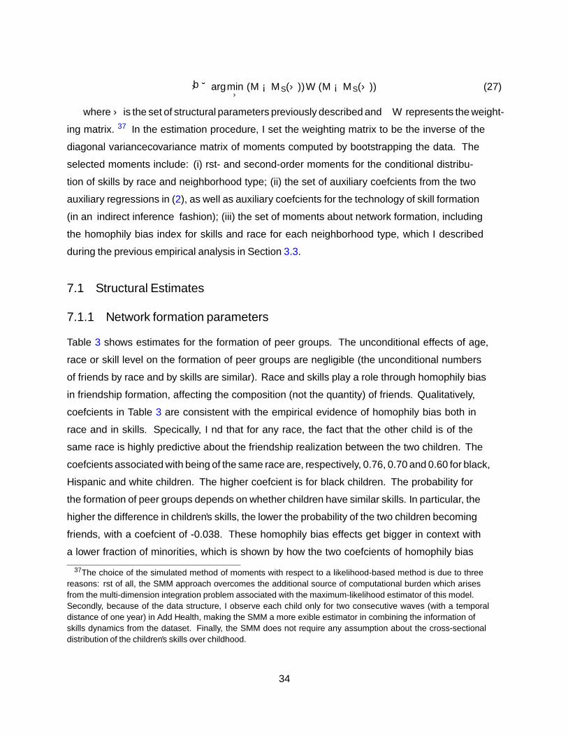
Ω= argminΩ

(M −MS(Ω))W (M −MS(Ω)) (27)

whereΩ is the set of structural parameters previously described and W represents the weight-

ing matrix.37 In the estimation procedure, I set the weighting matrix to be the inverse of the

diagonal variance–covariance matrix of moments computed by bootstrapping the data. The

selected moments include: (i) first- and second-order moments for the conditional distribu-

tion of skills by race and neighborhood type; (ii) the set of auxiliary coefficients from the two

auxiliary regressions in (2), as well as auxiliary coefficients for the technology of skill formation

(in an indirect inference fashion); (iii) the set of moments about network formation, including

the homophily bias index for skills and race for each neighborhood type, which I described

during the previous empirical analysis in Section 3.3.

7.1 Structural Estimates

7.1.1 Network formation parameters

Table 3 shows estimates for the formation of peer groups. The unconditional effects of age,

race or skill level on the formation of peer groups are negligible (the unconditional numbers

of friends by race and by skills are similar). Race and skills play a role through homophily bias

in friendship formation, affecting the composition (not the quantity) of friends. Qualitatively,

coefficients in Table 3 are consistent with the empirical evidence of homophily bias both in

race and in skills. Specifically, I find that for any race, the fact that the other child is of the

same race is highly predictive about the friendship realization between the two children. The

coefficients associated with being of the same race are, respectively, 0.76, 0.70 and 0.60 for black,

Hispanic and white children. The higher coefficient is for black children. The probability for

the formation of peer groups depends on whether children have similar skills. In particular, the

higher the difference in children’s skills, the lower the probability of the two children becoming

friends, with a coefficient of -0.038. These homophily bias effects get bigger in context with

a lower fraction of minorities, which is shown by how the two coefficients of homophily bias

37The choice of the simulated method of moments with respect to a likelihood-based method is due to threereasons: first of all, the SMM approach overcomes the additional source of computational burden which arisesfrom the multi-dimension integration problem associated with the maximum-likelihood estimator of this model.Secondly, because of the data structure, I observe each child only for two consecutive waves (with a temporaldistance of one year) in Add Health, making the SMM a more flexible estimator in combining the information ofskills dynamics from the dataset. Finally, the SMM does not require any assumption about the cross-sectionaldistribution of the children’s skills over childhood.

34

interact with the total fraction of black and white children (0.042 and -0.063, respectively). I

find that the correlation of unobservable heterogeneity in the formation of peer groups with

the production shocks is -0.40, while its standard deviation is 0.11. I do not find relevant effects

of the specific race or skills level in the probability level (only through homophily bias).

To better interpret the estimates, I plot the marginal probabilities of two children becoming

friends over the spectrum of children’s skills and for different races of children living in the

poorest environment (see Figure 4). For a black low-skilled child (within the first quintile of

skills distribution), the probability of becoming friends with white children is four times lower

than with a same-race counterpart. At the same time, it is two times more likely for the same

child to become friends with children having similar skills than for children in the top decile of

skills distribution. For a white low-skilled child (within the first quintile of skills distribution),

the racial gap is lower (around 2.5 times), while the effect of skills is similar.

7.1.2 Technology parameters

Table 4 shows estimates for the technology of skill formation. I find a high degree of static

substitutability between parents and peers, with a complementarity parameter (α3) of approx-

imately 0.95 (and associated elasticity of substitution of 11−0.95 = 20). I find a degree of self-

productivity (α1), i.e. the ability of skills to beget skills, of 0.75. This means that a 1% increase in

current skills would predict an average of 0.75% . This result is qualitatively in line with the pre-

vious research on the estimation of technology of skill formation (Cunha and Heckman, 2007,

2008; Cunha et al., 2010; Agostinelli and Wiswall, 2016). The magnitudes of the share paramet-

ers are meaningless due to the different scale between peers’ skills (normalized at age 13 to

have unit variance) and investments (in yearly hours). However, I find that the estimated value

of 0.009 implies that to completely offset a change of one standard deviation in peers’ skills, par-

ental investments need to change by approximately four hours per week (for the mean parent).

The return to scale of the combined parents–peers inputs (α4) is 0.77, suggesting non-linear

peer effects in skills dynamics even when parents and peers are approximately perfect substi-

tutes (linear). I find that the total factor productivity is an increasing function of the neigh-

borhood quality (γ1,t f p =0.008) and of the age of children (γ2,t f p =0.030). The coefficients for

school quality represent each neighborhood-type mean and standard deviation of the school

fixed effects. I find that average school quality is increased by neighborhood type (from -0.03

for low-income neighborhoods to 0.04 for high-income neighborhoods), while the standard de-

viation is decreased (from 0.26 for low-income neighborhoods to 0.18 for high-income neigh-

35

borhoods). Finally, I find production shocks to be important in explaining the total variation in

skills dynamics, with a coefficient for the standard deviation of shocks (σξ) of 0.70.

7.1.3 Preferences Parameters

Panel A in Table 5 shows estimates for preference parameters. I find both utility for consump-

tion and a child’s skills to be relatively concave, with a higher degree of curvature for consump-

tion relative to a child’s skills. I find a relatively high degree of parental altruism towards a child’s

skills: parents care about their child’s skills through ages 13 to 15 almost as much as their own

consumption, while they care twice as much about the final continuation value for their child

relative to their own current consumption. The last result underlines the importance of allow-

ing for a different parameterization for the final period preference, which, as explained above,

can capture a different developmental process for children, such as finishing high school, start-

ing a job or going to college.

7.1.4 Wage-Income Process and Initial Conditions

Panel B in Table 5 shows estimates for the wage and non-labor income process. A mother’s skills

are very predictive of both, suggesting an elasticity of 0.44 and 1.03 for wages and non-labor.

Table 6 shows estimates for the initial conditions by neighborhood type (low/medium/high

family income). The normalized mean and variance for a mother’s skills and a child’s initial

skills are for white families living in a low-income neighborhood (neighborhood 1). The other

subpopulations’ means and variances are relative to the normalized ones. I find that children

from minorities start with a lower mean of initial skills relative to their reference white chil-

dren. White children living in a higher family income neighborhood (neighborhoods 2 or 3)

have higher mean initial skills relative to white children in lower-income neighborhoods. I find

similar patterns in terms of mother’s skills.

7.2 Sample Fit

Table B-2 and Table B-3 report the sample fit for the auxiliary regressions of investments and

the dynamics of a child’s skills. The model is able to replicate the empirical findings on par-

ental investments and skill dynamics. Table B-2 also reports the 95% confidence interval to

show that the simulated coefficients are not statistically different from the fitted coefficients.

More importantly, Table B-2 shows that the model is able to replicate the switch in sign in

36

the peers’ skills, from the cross-sectional (negative) to the permanent (positive) variation in

peers, through the different degrees of static versus dynamic complementarity of parental in-

vestments and peers’ skills in skill formation.

Table B-3 shows that the estimated model is able to fit the auxiliary coefficients for the dy-

namic aspect of skill formation, suggesting that the estimated technology of skill formation

provides the proper marginal productivity for the developmental inputs. The reported 95%

confidence intervals suggest that the data and simulated coefficients are not statistically differ-

ent.

In terms of neighborhood effects on child development, the estimated model is able to fit

the differential patterns of skill formation between different neighborhoods and for different

races. Figures B-2-B-7 show the sample fit for the mean and standard deviation of skills by age,

race and for each of the three types of neighborhood I consider (low/medium/high income).

Figures B-8-B-9 show the sample fit for the homophily bias index for skills and race in dif-

ferent neighborhoods (low/medium/high income). Figure B-8 shows that the model tracks the

findings on the skills homophily bias in friendship formation. The model replicates the fact that

high-skilled children display a higher bias toward children with similar skills.

Figure B-9 shows that the model is able to replicate the findings of homophily bias by race

in different neighborhoods. However, within the high-income neighborhood, while the data

indicate a fall in the homophily bias index for Hispanic children relative to black children, the

model indicates a common tendency of homophily bias between the two races.

8 The Exposure Effects of Environments on Child Development

In this section, I analyze the extent to which environments explain differences in children’s fi-

nal achievements. In order to calculate the treatment effect of better environments, I simulate

the counterfactual dynamics of skills as the outcome of being moved to a different environ-

ment. I compute the treatment effect by simulating each child in each different environment

and school and at any age I consider in the model.

Within the estimated model, I can now calculate the treatment effect of moving from any

considered environment to any of the others. Specifically, consider the case where a child i

is permanently moved from a environment e to a environment e’ at age m. The individual

treatment effect in this case is:

T Ei (e,e’,m) = y∗i (e,e’,m)− y∗

i (e) (28)

37

where y∗i (e) represents the baseline child percentile in the skill distribution at age 16, while

y∗i (e,e’,m) represents the child percentile in the skill distribution at age 16 if the child is moved

from her original environment e to a new environment e’ at age m. To simplify the analysis and

to have a comparable setting with the previous literature, I first characterize environments by

their mean percentiles of skills of permanently based children at age 16 (ye ). Second, I consider

a specific parametric relationship between a child’s outcome and the associated mean percent-

iles of children’s skills at age 16 in each environment (ye ):

y∗i =ψ0 +ψ1,m ye +εi (29)

where ye represents the associated mean percentile of children’s skills in environment e. In

this case, ψ1,m represents the average treatment effect of being permanently moved at age m

from a environment e to a new environment e’ which has a mean of children’s skills at age 16

that is one percentile higher.

Finally, I can compute the exposure effects of environments, which represent the effects on

skill formation of an additional year in a environment with a mean of children’s skills at age 16

that is one percentile higher. Following equation (29), the exposure effects are simply ψ1,m -

ψ1,m+1.

Figure 5 shows that environments have sizable effects on skill formation. Moving a child at

age 12 into a environment with a mean of children’s skills at age 16 that is one percentile higher

causes an increase of her skills by approximately 0.65 percentiles. This effect declines by age. I

find an exposure effect of 0.048, which means that the outcomes of moved children converge

to the outcomes of receiving children at a rate of 4.8% per year of exposure. In other words,

moving a child to a better environment at 14 rather than at 13 years old causes the child to lose

almost 5% of the benefit of moving. The exposure effects imply approximately a 15% higher

benefit from moving to the same environment at 12 rather than at 15 years old.38

8.1 Model Validation: Comparison with Exposure Effects in Chetty and Hendren

(2016a)

The specification in (29) allows me to compare my results with those in Chetty and Hendren

(2016a). The authors implement the same specification to analyze the childhood exposure

38My model starts at age 13 when children draw their skills after the realization of the environment where theylive. In this exercise, when I move children at age 12, it means that I allow children to be in the environment beforethey draw their skills. In contrast, when I move them at age 13, I let them first draw their skills in the originalenvironment and then move them into the new environment.

38

effects of environments for the United States. The authors consider individual income per-

centiles at age 24 as their variables of interest. Still, my results are comparable with those in

Chetty and Hendren (2016a) under the reasonable assumption that expected individual income

is defined by any monotone rank-preserving function of children’s skills (higher skills imply av-

erage higher individual income).39

Figure 5 shows that my model tracks the findings in Chetty and Hendren (2016a), who find

that an additional year of exposure to a environment with a mean income of one percentile

higher for permanently moved children increases a child’s income later in life by approxim-

ately 0.04 percentiles. The authors also find exposure effects to be stronger for families above

the median income distribution. Table 7 shows the comparison of model predictions and their

estimates with respect to family income. The model’s predictions are in line with the hetero-

geneous exposure effects.

It is still an open question, however, as to which factors drive the exposure effects. In the

next section, I decompose the overall exposure effects into three classes of environment-specific

amenities: peers, school quality and environment quality.

8.2 Decomposition of Childhood Exposure Effects

One advantage of my structural model is that I can now decompose the previous findings of

exposure effects with respect to each of the components which characterized an environment

in my model: peers, school quality and environment quality.

With the estimated model, I can replicate the previous simulated experiment of moving chil-

dren within different scenarios to isolate the effects of each of the previous inputs. I first move

children and compute the treatment effect of moving to different environments at different ages

due exclusively to the associated change of peers (keeping the previous level of both school and

environment quality fixed). Secondly, I compute the effect of moving children when the asso-

ciated treatment is composed by both changes in peers and the new school quality (keeping

the previous level of environment quality fixed). Finally, I calculate the overall treatment effect

of moving at different ages associated with the new peers, the new school and the new envir-

onment quality. In this way, I can ascertain the contribution of each component to the overall

effects of childhood exposure to environments.

Table 8 shows the decomposition of the overall effect. Peers alone account for more than

39 I could also estimate a relationship between individual income at age 24 and children’s skills at age 16 and thenuse this estimated function to predict individual income for the simulation exercise. Any monotone relationshipbetween these two variables would give me the same results in terms of rank effects.

39

half of the childhood exposure effects, while school and environment quality account for the

rest. This means that more than half of the effect of an additional year in a environment with

mean skills one percentile higher for permanently moved children is caused by the child’s so-

cial interactions. Whether a child leaves a disadvantaged environment affects the quality of

the child’s social interactions (in terms of peers’ skills). The dynamic complementarity of skill

formation causes this effect to have a higher return earlier than later throughout adolescence.

Each additional year of adolescence spent in an environment with mean skills one percentile

lower for permanently moved children worsens the child’s skills at age 16 by 0.027 percentiles,

exclusively through social interactions. The exposure to the same social interactions from age

12 to age 15 would cause a reduction of skills by approximately 0.08 percentiles.

The overall exposure effects are bigger for disadvantaged children, and in this case, peer ef-

fects account for almost two-thirds. Children who have a low endowment of skills and are from

lower-income families are more likely to live in low-income environments, where they have

higher chances of interacting with low-skilled peers due to the homophily bias effects in peer-

group formation. This channel explains why this group of children experiences the greatest

benefit from leaving these disadvantaged environments. The exposure effect in this case is

approximately 0.05, and peers alone account for up to 60% of this finding. For this specific

subgroup of children from low-income families, each additional year of adolescence spent in

an environment with mean skills of one percentile lower for permanently moved children wor-

sens a child’s skills by around 0.034 percentiles at age 16, exclusively through social interactions.

Figure 6 shows graphically the same result for lower-skilled children.

These results suggest the importance of social interactions alone in explaining the differ-

ences in developmental trajectories in children from different environments. In the next sec-

tion, I analyze the effects of policies that target disadvantaged children and change the peers’

composition between different environments, for example, policy that promote socioeconomic

integration between environments or schools.

9 Policy Analysis

The decomposition of the exposure effects of environments suggests that more than half of

the effects come from peers and social interaction. This result calls for policies which focus

on changes in peers’ composition between different environments to overcome the negative

effects of growing up in disadvantaged environments. I analyze how this kind of policy, if im-

plemented on a large scale (i.e. when a sizable fraction of children are moved into a new envir-

40

onment), can generate important equilibrium effects in skill dynamics through the changes in

social interactions.

9.1 Large Scale Changes in Peers’ Composition

The estimated model reveals that skills dynamics depend on a peers’ composition and associ-

ated children’s social interactions. In this section, I analyze the quantitative equilibrium effects,

created by policies that change cohort compositions into different social contexts, on the dy-

namics of skills. Specifically, I want to understand the implications of changes in cohort com-

positions within both receiving and sending environments. In order to answer this question,

I perform a simulated counterfactual analysis where I move disadvantaged children (and their

parents), i.e. children with low skill endowment at age 13 and living in a poor environment, into

a high-income environment. This policy has diverse effects on three subgroups of people: (i)

parents and children who are moved; (ii) parents and children who live in the receiving (high-

income) environment; (iii) parents and children who remain in the low-income environment.

The simulated policy targets a specific group of disadvantaged children: children who are

within the first quartile of skills distribution at age 13 in the low-income environment. More

than 70% of these children are from a racial minority and their initial (age 13) skills are, on

average, about a standard deviation below the population mean of log-skills at age 13. On the

other hand, the racial composition of the receiving environment is different: the racial minority

makes up only 18% of the population. On average, receiving children are 0.12 standard devi-

ations above the population mean of children’s log-skills at age 13. I consider the policy effects

when the moved children group is about 5% and 30% of the receiving cohort. These sizable

changes in cohort composition allows me to analyze the equilibrium effects of the policy. In the

last part of this section, I will discuss more in detail how the effects change as a function of the

fraction of moved children.

Table 9 shows the effects of the policy that moves the smaller fraction of children (5% of the

receiving population). Panel A reports the effects of the policy on children’s skills for both the

moved and receiving children. For each group, I report the baseline as well as the counterfactual

skill dynamics. To assess the importance of equilibrium effects, I also report the counterfactual

results without any dynamic equilibrium effects (column called “No Equilibrium”). In this case,

I just solve the parent’s behavioral problem without considering any equilibrium feedback ef-

fects from the endogenous response of other parents’ behavior after the policy change. The first

finding is that this policy has small effects for the receiving children, with a minimal decrease

41

in skills at age 16 of 3%. On the other hand, I find that moved children increase their skills at

age 16, on average, by 55% (0.4 of a standard deviation of children’s skills at age 16).40

Panel B in Table 10 shows the effects of the policy change on parental investment decisions.

I find that parents of moved children increase their investments overall, fostering the effects of

the policy on their own child’s skills dynamics. On the other hand, parents of receiving children

do not respond to changes in peer composition.

Table 10 displays the effects for the larger policy. Panel A in Table 10 reports the effects of the

policy on children’s skills also for the remained children. In this case, the policy creates winners

and losers: an average increase in skills at age 16 of 31% and 23%, respectively, for moved and

remaining children is associated with an average decline of 15% in receiving children. An al-

ternative interpretation of the results is in terms of the standard deviation of skills distribution:

I find that moved and remaining children increase their log-skills on average by 0.22 and 0.17,

respectively, of a standard deviation of children’s log-skills at age 16, while, on average, log-skills

for receiving children decrease approximately by 0.10 of a standard deviation. The results sug-

gest that children who remained in the sending environment benefit from the outflow of the

most disadvantaged companions.

Panel B in Table 10 shows the effects of the policy change on parental investment decisions. I

find that parents of receiving children reduce their engagement with children due to a lower ex-

pected level of peers’ skills. On the contrary, parents of moved and remaining children increase

their investments due to the policy (positive) change in the expected future peers. Indeed, as

suggested by the instrumental variable results, a positive (negative) permanent change in peer

composition induces a positive (negative) change in investments due to the dynamic comple-

mentarity. Figure 7 illustrates how the policy change has affected the equilibrium endogenous

distribution of peers’ skills and the relative parents’ expectations, causing parents with better

(worse) expectations to increase (decrease) their investments.

Finally, Table 9 and Table 10 underline the importance of accounting for equilibrium ef-

fects in this type of policy analysis. I find that equilibrium feedback effects tend to amplify the

policy effects, and ignoring those would lead to biased policy predictions for children’s final

skills of approximately seven times smaller. Part of this gap is due to the erroneous predictions

for investment decisions: in the absence of dynamic-equilibrium feedback effects, the static

complementarity between parents and peers dominates the dynamic effects of the policy. In

this case, a positive (negative) change in peer composition induces a negative (positive) change

in investments.40The national population’s standard deviation of children’s log-skills at age 16 is 1.37

42

9.1.1 Heterogenous Effects

In this section, I analyze whether the larger counterfactual policy (when the moved children

group is 30% of the receiving cohort) generates heterogeneous effects between children due

to the new counterfactual social network. I focus my attention to the two sources of potential

homophily bias: skills and race. Figure 8 shows the return of policy (treatment effect) in % of

skills at age 16 for different children in terms of their initial endowment of skills at age 13. The

x-axis displays the percentiles of initial skill endowment for each subgroup. I find that children

with lower skills at age 13 benefit the most when moved to a better environment. The treatment

effect for children in the first decile of skills within the group of moved children is between 32%-

35% in skills at age 16 (approximately 0.25 of a standard deviation for log-skills at age 16). This

result is clear evidence of the role of segregated social interactions in child development: in the

absence of context-specific network formation, the CES technology in (4) would predict that

return of policy would increase in a child’s endowment.41 However, a discontinuous policy-

induced change in peers creates higher benefits for children who are moved away from adverse

social interactions. The policy induces a lower return for children with better initial skills, with

the bottom of the effects of approximately 24% for children above the median of the moved

group.

The heterogeneous effects in Figure 8 for receiving children reveal the importance of the

counterfactual endogenous network formation. I find that children in the lower part of the skills

distribution have the most sizable adverse effects within the group of receiving children. The

treatment effect in this case is -0.14 of a standard deviation of log-skills at age 16. In fact, this

group of children is the most exposed to social interactions with the new potential peers. For

the same reason as the counterfactual change in social interactions, Figure 8 suggests that the

policy return for children in the sending (low-income) environment are higher for low-skilled

children, with a policy effect of approximately 0.20 of a standard deviation of log-skills at age 16

for children in the first skill decile, in contrast with 0.13 of a standard deviation for children in

the highest decile.

Evidence from previous empirical studies indicates a potential racial difference in peer ef-

fects in children, pointing out that peer effects seem to be stronger intra-race and for minorities

(see for example Hoxby, 2000; Angrist and Lang, 2004; Imberman et al., 2012).42 My quantitat-

41This is because of the assumed complementarity between a child’s endowment and other inputs: ∂2θt+1

∂θt∂H i ,t≥ 0.

42Imberman et al. (2012) exploit the Katrina natural experiment to evaluate peer effects in receiving schools inLouisiana and Houston. The authors find negative peer effects on school attendance, disciplinary infractions andmath scores for black children, although the last effect is statistically imprecise

43

ive exercise confirms the previous literature’s results. Table 11 shows the decomposed results

for receiving children by race. Children from minority groups are most adversely affected by

the policy, with a reduction of approximately 42% and 35% (-0.30 and -0.25 of a standard devi-

ation) of log-skills at age 16 for black and Hispanic children, respectively. On the other hand,

I find that the effects on white children are smaller, with a reduction of log-skills at age 16, on

average, of approximately 11% (0.08 of a standard deviation).43 Panel B in Table 11 shows the

counterfactual parental investment behavior. Again, groups that are more exposed to the per-

manent change in cohort composition (through homophily bias in social interactions) sizably

reduce their parental involvement due to the dynamic complementarity between their current

choice and the expected future peers.

9.1.2 The Scale Effects of Policy

During the previous policy analysis, I analyzed the effects of moving two different fractions of

disadvantaged children into a high-income environment: 5% and 30% of the receiving pop-

ulation. Equilibrium effects on both receiving and sending environments were quantitatively

different. In this section, I analyze the different implications for the same counterfactual policy

as a function of different fractions of moved children. Specifically defining the original moved

group as the eligible children, I now compute the equilibrium effects of the policy relative to the

fraction of eligible children who are actually moved.

Figure 9 reports the average effects on children’s log-skills at age 16 in the counterfactual

economy as a function of the fraction of eligible moved children (x-axis) for the three subgroups

of interest (moved, receiving and remaining children). The first result is that both the moved

and receiving children are better off if the policy provides a relatively small group of moved

children. For moved children, the return of the policy rapidly drops as the fraction of eligible

children rises in the new environment. Moving 3% or 30% of children creates a difference of

approximately 20% in the final skills for moved children. This suggests that the probability of

children from the same original environment continuing to interact with each other in the new

social context is still high. For the receiving children, the decline is more gradual. The total

change between moving nobody versus moving 30% of eligible children is approximately 15%,

and it monotonically declines as more eligible children are moved into the environment. The

second result is that the remaining children gain increasingly more out of the policy if the frac-

tion of disadvantaged children who are moved out from that environment increases. A gain of

43The heterogeneous treatment effects by race for the smaller policy are qualitatively similar, see Table B-4

44

40% is guaranteed for remaining children if 30% of children are moved out from that environ-

ment. An increased outflow of the most disadvantaged children from the sending environment

benefits children who remain, which is a result of the positive effects of the new peers’ skills.

9.2 The Persistent Effects of Social Environments on Skills Dynamics

The last quantitative analysis focuses on underlining the persistent effects on skill dynamics

of growing up in disadvantaged environments. To answer this question, I perform a simulated

counterfactual policy which targets the same disadvantaged group of children as before, but

now I boost their initial endowment at age 13 while keeping them living in the low-income en-

vironment. I compare their dynamics of skills throughout childhood with children with similar

initial skills but living in better environments.

Table 12 reports the counterfactual results. I find that living in different social contexts per-

manently shapes the developmental trajectories of children. In particular, after starting from

the same initial endowment, the dynamics of skills in the disadvantaged environment fail to

keep up with the skills dynamics of children from the high-income environment. The growth

rate of skills is approximately 60% higher for children in the higher-income environment dur-

ing the age of 13–14 years, while at the end, the two groups’ growth rates in skill converge. This

leads to a total difference, at age 16, of approximately 57% in final skills.

Social interactions and children’s skills composition play an important role in explaining

this result. First, children living in the low-income environment have, on average, lower-skilled

peers than children living in the high-income environment. Secondly, the two different social

contexts determine parents’ different expectations about their child’s social interactions with

peers, thus affecting their investment behavior.

Panel B in Table 12 shows that parents increase engagements with their offspring as the res-

ult of a higher initial skill endowment of their child. However, they are far from the parental

investment levels of parents in high-income environments. The difference is approximately

between 4 and 6 percentage points in terms of time allocated to child development. Figure 10

shows that part of this investment gap is due to differences in the expected peer effects through-

out childhood. Hence, social influences determine patterns of skill inequality and, again, one

key mechanism is the dynamic complementarity between parents and expected peers.

45

10 Conclusion

This paper studies the role of children’s social interactions in the dynamics of children’s skills. I

estimate a tractable dynamic equilibrium model of parental investment and endogenous form-

ation of peer groups. The model is estimated using information about friendships, children’s

test scores and parental investments in the National Longitudinal Study of Adolescent Health

(Add Health). I exploit within school / across cohort variations in peers’ composition to identify

the degree of complementarity between parents and peers in producing a child’s skills. I find

that parents and peers are static substitutes and dynamic complementary inputs in child de-

velopment. After validating my estimated model using findings in Chetty and Hendren (2016a)

on environment exposure effects in children, I assess the importance of social interactions in

skills dynamics with various policies.

This article underlines three main points: (i) social interactions and social context perman-

ently shape the developmental trajectories of children; (ii) changing cohort composition and

the relative social interactions generates winners and losers and the heterogeneous effects are

due to the endogenous formation of new peers; (iii) neglecting the dynamic equilibrium effects

of skill formation and social interactions would lead to biased predicted effects of policies.

I want to conclude this paper by considering an extension of this work. Specifically, one po-

tential type of parental investment can be the choice of neighborhood where the family lives. In

this case, parents have alternative margins in response to changes in peer composition, and to

a certain extent, they can also decide to change where they live as a response to the previously

considered policy. Modeling this second channel is challenging, because now the environment

composition is also endogenous, and it becomes part of the equilibrium solution of the model.

However, understanding the extent to which neighborhood decisions are influenced by chil-

dren’s social interactions is an important question in considering the effects of socioeconomic

segregation on intergenerational mobility. Therefore, future work is needed.

46

References

Atila Abdulkadiroglu, Joshua D. Angrist, and Parag A. Pathak. The elite illusion: Achievement

effects at Boston and New York exam schools. Econometrica, 82:137–196, 2014.

Francesco Agostinelli and Matthew Wiswall. Estimating the technology of children’s skill form-

ation. NBER Working Paper n. 22442, 2016.

Andreas Ammermueller and Jörn-Steffen Pischke. Peer effects in european primary schools:

Evidence from the progress in international reading literacy study. Journal of Labor Econom-

ics, 27(3):315–348, 2009.

Donald W. K. Andrews and Gustavo Soares. Inference for parameters defined by moment in-

equalities using generalized moment selection. Econometrica, 78(1):119–157, 2010.

Joshua D. Angrist and Kevin Lang. Does school integration generate peer effects? Evidence from

Boston’s METCO program. American Economic Review, 94(5):1613–1634, 2004.

Peter Arcidiacono, Gigi Foster, Natalie Goodpaster, and Josh Kinsler. Estimating spillovers using

panel data, with an application to the classroom. Quantitative Economics, 3:421–470, 2012.

Orazio Attanasio, Sarah Cattan, Emla Fitzsimons Costas Meghir, and Marta Rubio−Codina. Es-

timating the production function for human capital: Results from a randomized controlled

trial in Colombia. NBER Working Paper n. 20965, 2017a.

Orazio Attanasio, Costas Meghir, and Emily Nix. Human capital development and parental

investment in India. NBER Working Paper n. 21740, 2017b.

Orazio Attanasio, Costas Meghir, Emily Nix, and Francesca Salvati. Human capital growth and

poverty: Evidence from Ethiopia and Peru. Review of Economic Dynamics, 25:234 – 259,

2017c.

Eric Auerbach. Identification and estimation of models with endogenous network formation,

2016.

Anton Badev. Discrete games in endogenous networks: Theory and policy. Working Paper,

2016.

Venkatesh Bala and Sanjeev Goyal. A noncooperative model of network formation. Economet-

rica, 68(5):1181–1229, 2000.

47

Robert Bifulco, Jason M. Fletcher, and Stephen L. Ross. The effect of classmate characteristics

on post-secondary outcomes: Evidence from the Add Health. American Economic Journal:

Economic Policy, 3(1):25–53, 2011.

Lawrence E. Blume, William A. Brock, Steven N. Durlauf, and Yannis M. Ioannides. Identific-

ation of social interactions. Handbook of Social Economics, J. Benhabib, A. Bisin, and M.

Jackson, Amsterdam: North Holland, 2011.

Lawrence E. Blume, William A. Brock, Steven N. Durlauf, and Rajshri Jayaraman. Linear social

interactions models. Journal of Political Economy, 123(2):444–496, 2015.

Yann Bramoullé, Habiba Djebbari, and Bernard Fortin. Identification of peer effects through

social networks. Journal of Econometrics, 150(1):41 – 55, 2009.

William A. Brock and Steven N. Durlauf. Interactions-based models. Handbook of Econometrics

by J. Heckman and E. Leamer, 5(Amsterdam: North-Holland):52–75, 2001a.

William A. Brock and Steven N. Durlauf. Discrete choice with social interactions. Review of

Economic Studies, 68(2):235–260, 2001b.

William A. Brock and Steven N. Durlauf. Linear social interactions models. Journal of Econo-

metrics, 140:52–75, 2007.

Mary A. Burke and Tim R. Sass. Classroom peer effects and student achievement. Journal of

Labor Economics, 31(1):51–82, 2013.

Antoni Calvó-Armengol, Eleonora Patacchini, and Yves Zenou. Peer effects and social networks

in education. Review of Economic Studies, 76(4):1239–1267, 2009.

David Card and Laura Giuliano. Can tracking raise the test scores of high-ability minority stu-

dents? American Economic Review, 106(10):2783–2816, 2016.

Scott E. Carrell, Bruce I. Sacerdote, and James E. West. From natural variation to optimal policy?

The importance of endogenous peer group formation. Econometrica, 81(3), 2013.

Scott E. Carrell, Mark Hoekstra, and Elira Kuka. The long-run effects of disruptive peers. NBER

Working Paper n. 22042, 2016.

Elizabeth M. Caucutt and Lance Lochner. Early and late human capital investments, borrowing

constraints, and the family, 2017.

48

Arun G. Chandrasekhar and Randall Lewis. Econometrics of sampled networks, 2016.

Victor Chernozhukov, Han Hong, and Elie Tamer. Estimation and confidence regions for para-

meter sets in econometric models. Econometrica, 75(5):1243–1284, 2007.

Raj Chetty and Nathaniel Hendren. The impacts of neighborhoods on intergenerational mobil-

ity I: Childhood exposure effects, 2016a.

Raj Chetty and Nathaniel Hendren. The impacts of neighborhoods on intergenerational mobil-

ity II: County-level estimates, 2016b.

Raj Chetty, Nathaniel Hendren, and Lawrence Katz. The effects of exposure to better neigh-

borhoods on children: New evidence from the moving to opportunity project. American

Economic Review, 106(4), 2016a.

Raj Chetty, Nathaniel Hendren, Frina Lin, Jeremy Majerovitz, and Benjamin Scuderi. Child-

hood environment and gender gaps in adulthood. American Economic Review Papers and

Proceedings, 2016b.

Nicholas A. Christakis and James H. Fowler. Connected: The surprising power of our social

networks and how they shape our lives. Little, Brown and Company, 2009.

Nicholas A. Christakis, James H. Fowler, Guido W. Imbens, and Karthik Kalyanaraman. An em-

pirical model for strategic network formation. NBER Working Paper n. 16039, 2010.

James S. Coleman. Relational analysis: the study of social organizations with survey methods.

Hum Organ, 17:28–36, 1958.

Flavio Cunha. Investments in children when markets are incomplete, 2013.

Flavio Cunha and James Heckman. The technology of skill formation. American Economic

Review, 97(2):31–47, 2007.

Flavio Cunha and James J. Heckman. Formulating, identifying, and estimating the technology

for the formation of skills. Journal of Human Resources, 43(4):738–782, 2008.

Flavio Cunha, James J. Heckman, and Susanne M. Schennach. Estimating the technology of

cognitive and noncognitive skill formation. Econometrica, 78(3):883–931, 2010.

49

Sergio Currarini, Matthew O. Jackson, and Paolo Pin. Identifying the roles of race-based

choice and chance in high school friendship network formation. Proceedings of the National

Academy of Sciences, 107(11), 2010.

Manjira Datta, Kevin Reffett, and Lukasz Wozny. Comparing recursive equilibria in economies

with dynamic complementarities and indeterminacy. Economic Theory, Forthcoming, 2017.

Giacomo De Giorgi, Michele Pellizzari, and Silvia Redaelli. Identification of social interactions

through partially overlapping peer groups. American Economics Journal: Applied Economics,

2(2):241–275, 2010.

Daniela Del Boca, Christopher Flinn, and Matthew Wiswall. Household choices and child de-

velopment. Review of Economic Studies, 81(1):137–185, 2014.

Daniela Del Boca, Christopher Flinn, and Matthew Wiswall. Transfers to households with chil-

dren and child development. Economic Journal, Forthcoming, 2016.

Bhaskar Dutta, Sayantan Ghosal, and Debraj Ray. Farsighted network formation. Journal of

Economic Theory, 122(2):143–164, 2005.

Chao Fu and Jesse Gregory. Estimation of an equilibrium model with externalities: Combining

the strengths of structural models and quasi experiments, 2017.

Chao Fu and Nirav Mehat. Ability tracking, school and parental effort, and student achieve-

ment: A structural model and estimation. Working Paper, 2016.

George-Levi Gayle, Limor Golan, and A. Mehmet Soytas. What accounts for the racial gap in

time allocation and intergenerational transmission of human capital?, 2015.

George-Levi Gayle, Limor Golan, and A. Mehmet Soytas. What is the source of the intergenera-

tional correlation in earnings?, 2016.

Paul Goldsmith-Pinkham and Guido W. Imbens. Social Networks and the Identification of Peer

Effects. Journal of Business & Economic Statistics, 31(3):253–264, 2013.

Bryan S. Graham. Homophily and transitivity in dynamic network formation, 2016.

Bryan S. Graham. An econometric model of network formation with degree heterogeneity. Eco-

nometrica, 85(4):1033–1063, 2017.

50

Alan Griffith. How many friends do you have? An empirical investigation into

censoring−induced bias in social network data, 2017.

Carolyn T. Halpern. Smarter teens delay sexual contacts. PPFY (Pregnancy Prevention for Youth)

Network Newsletter, 3:4–5, 2000.

Eric A. Hanushek, John F. Kain, Jacob M. Markman, and Steven G. Rivkin. Does peer ability

affect student achievement? Journal of Applied Econometrics, 18(5):527–544, 2003.

James J. Heckman and Dimitriy V. Masterov. The productivity argument for investing in young

children. Review of Agricultural Economics, 29(3):446–493, 2007.

Caroline Hoxby. Peer effects in the classroom: Learning from gender and race variation. NBER

Working Paper n. 7867, 2000.

Scott A. Imberman, Adriana D. Kugler, and Bruce I. Sacerdote. Katrina’s children: Evidence on

the structure of peer effects from hurricane evacuees. American Economic Review, 102(5):

2048–2082, 2012.

Matthew O. Jackson. Social and Economic Networks. Princeton University Press, 2008.

Matthew O. Jackson and Asher Wolinsky. A strategic model of social and economic networks.

Journal of Economic Theory, 71(1):44–74, 1996.

Victor Lavy and Analia Schlosser. Mechanisms and impacts of gender peer effects at school.

American Economic Journal: Applied Economics, 3(2):1–33, 2011.

Victor Lavy, M. Daniele Paserman, and Analia Schlosser. Inside the black box of ability peer

effects: Evidence from variation in the proportion of low achievers in the classroom. The

Economic Journal, 122(559):208–237, 2012.

Natalia Lazzati. Treatment response with social interactions: Partial identification via mono-

tone comparative statics. Quantitative Economics, (6):49–83, 2015.

Charles F. Manski. Identification of endogenous social effects: The reflection problem. Review

of Economic Studies, 60(3):531–542, 1993.

Angelo Mele. A structural model of segregation in social networks. Working Paper, Net Institute

(10-16), 2010.

51

Jacob Mincer. Investment in human capital and personal income distribution. Journal of Polit-

ical Economy, 66(4):281–302, 1958.

Joseph Mullins. Improving child outcomes through welfare reform, 2016.

Claudia Olivetti, Eleonora Patacchini, and Yves Zenou. Mothers, peers and gender identity.

Working Paper, 2016.

Ariel Pakes, J. Porter, Kate Ho, and Joy Ishii. Moment inequalities and their application. Econo-

metrica, 83(1):315–334, 2015.

Eleonora Patacchini and Yves Zenou. Juvenile delinquency and conformism. Journal of Law,

Economics and Organization, 28(1):1–31, 2012.

Eleonora Patacchini and Yves Zenou. Social networks and parental behavior in the intergener-

ational transmission of religion. Quantitative Economics, 7:969–995, 2016.

Eleonora Patacchini, Edoardo Rainone, and Yves Zenou. Student networks and long-run edu-

cational outcomes: The strength of strong ties. CEPR Discussion Papers 9149, C.E.P.R. Discus-

sion Papers, 2012.

Bruce Sacerdote. Peer effects with random assignment: Results for Dartmouth roommates. The

Quarterly Journal of Economics, 116:681–704, 2001.

Bruce Sacerdote. Experimental and quasi-experimental analysis of peer effects: Two steps for-

ward? Annual Review of Economics, 6:253–272, 2014.

Shuyang Sheng. A structural econometric analysis of network formation games. Working Paper,

2014.

Petra Todd and Kenneth Wolpin. On the specification and estimation of the production func-

tion for cognitive achievement. Economic Journal, 113(3):F3–F33, 2003.

Petra Todd and Kenneth Wolpin. The production of cognitive achievement in children: Home,

school, and racial test score gaps. Journal of Human Capital, 1(1):91 – 136, 2007.

Donald M. Topkis. Equilibrium points in nonzero-sum n-person submodular games. SIAM

Journal of Control and Optimization, 17(6):773–787, 1979.

52

Table 1: Sample Statistics

Mean StandardDeviation

(1) (2)

Child’s Age 15.65 1.74Fraction black 0.16 0.37Fraction hispanic 0.17 0.38Fraction white 0.67 0.47N of reported friends (In-School) 4.48 3.58

Measures for skills:

PPVT 64.26 11.14English 2.83 0.98Math 2.72 1.03History 2.86 1.01Science 2.82 1.01

Family’s characteristics:

Income ($ 1994) 42,844 27,724Mother’s education 13.13 2.35

Measures for parental investments :(activities in the last 4 weeks with mother)

Gone shopping 0.72 0.44Played a sport 0.08 0.28Gone to a religious service 0.38 0.49Talked about someone you are dating 0.47 0.50(or a party you went to )Gone to a movie, play, museum, concert, or sports event 0.25 0.44Had a talk about a personal problem you were having 0.39 0.49Had a serious argument about your behavior 0.33 0.47Talked about your school work or grades 0.63 0.48Worked on a project for school 0.13 0.34Talked about other things you are doing in school 0.54 0.50

Notes: This table reports the descriptive statistics for the sample I use in the estimation of themodel. The number of reported friends is the number of nominated friends during the survey.The measures for parental investments are binary variables, which take value one if the activitywas done, zero otherwise.Data source: National Longitudinal Survey of Adolescent Health (Add Health).

Table 2: Parental Investments, Child’s and Peers’ Skills

Dependent Variable

Fraction (%) of Invested Parental Time

(1) (2)Measurement Error Adjusted Measurement Error Adjusted

andInstrumental Variables (IV)

Child Skills (Log) 2.660 2.120(0.316) (0.668)

Peers’ Skills (Log) -1.441 0.720(0.650) (0.354)

N of Children 14,267 14,267

Age Fixed Effects X XSchool’s Fixed Effects X X

Panel B: First Stage

Z1,i ,t (Minorities Children) -0.104(0.052)

Z2,i ,t (White Children) 0.082(0.037)

F-Stat Excl. Instruments 11.78P-value 0.000

Notes: This table shows estimates for both model 2 (column 1) and 2 (column 2). The dependent variable isthe fraction of invested parental time at age t and the covariates (log skills and log peers’ skills) are at also attime t . All models also include controls for children’s race, mother’s skills and lagged family income. Standarderrors in parenthesis are computing using a cluster bootstrap. The first stage statistics in column 2 shows thecoefficients (and standard errors in parenthesis) of both excluded instruments for the first stage as well as theF-statistic of the joint null hypothesis that both coefficients are zero. Stock and Yogo provide critical values totest weak IV condition based on the F-stat of excluded instruments. Those critical values can be interpreted asa test with a 5 % significance level, of the hypothesis that the maximum relative bias (with respect to the OLSestimates) is 10% or at least 15%. In this case, the Stock and Yogo critical values for the F-stat of the excludedinstruments are 19.93 (10%) and 11.59 (15%).Data source: National Longitudinal Survey of Adolescent Health (Add Health).

Table 3: Estimates for the Network Formation Model

Parameter Estimate S.E.

Constant (δ1) -0.246 0.0172

Child‘s Log-Skills (δ2) 0.088 0.0048

Black (δ3,1) 0.075 0.0023

Hispanic (δ3,2) -0.005 0.0001

Both Black (δ4,1) 0.763 0.0317

Both Hispanic (δ4,2) 0.701 0.0298

Both White (δ4,3) 0.559 0.0475

Distance in Children‘s Skills (δ5) -0.038 0.0014

N of Children (Hundreds, δ6,1) -0.890 0.0003

N of Children Squared (Hundreds, δ6,2) 0.001 0.0000

Distance in Children‘s Skills · %White (δ6,3) - 0.063 0.0032

Distance in Children‘s Skills · %Black (δ6,4) 0.042 0.0025

Age (δ7) -0.050 0.0010

Additional Unobserved Heterogeneity (ζi , j ,t )

Correlation with Skill Shocks -0.404 0.0212

Standard Deviation 0.110 0.0095

Notes: This table shows the structural estimates for the child’s utility for friend-ships in Equation (5). The child’s utility shock is defined as νi , j ,t = νi , j ,t + ζi , j ,t ,where ζi , j ,t and is correlated with the production function shock (ξi ,t ). The lastpart of the table shows the estimated correlation and standard deviation σζ. Thestandard errors are computed using a cluster bootstrap.

Table 4: Estimates for the Technology of Skill Formation

Parameter Estimate S.E.

Child‘s Skills (α1) 0.744 0.0682

Investments (Yearly Hours, α2) 0.009 0.0014

Elasticity Investment vs Peers (α3) 0.944 0.0270

Return to Scale (α4) 0.767 0.0283

Std of Shocks (σξ) 0.700 0.0461

Panel B: TFP

Constant (γ0,t f p ) -1.329 0.1256

Neighborhood Quality (γ1,t f p ) 0.008 0.0003

Age Trend (γ2,t f p ) 0.030 0.0008

Panel C: School-Quality Effects

Low Income Neighborhood

Mean (ηs,1) -0.033 0.0350

Standard Deviation (σs,1) 0.262 0.0264

Medium Income Neighborhood

Mean (ηs,2) 0.006 0.0277

Standard Deviation (σs,2) 0.244 0.0278

High Income Neighborhood

Mean (ηs,3) 0.041 0.0318

Standard Deviation (σs,3) 0.188 0.0249

Notes: This table shows the estimates for the technology of childrenskill formation in Equation (17). Panel B reports the parameter es-timates for the neighborhood-specific TFP defined in Section 5.2.Panel C reports the mean and standard deviation of school-qualityfor each neighborhood type. The standard errors are computed us-ing a cluster bootstrap.

Table 5: Estimates for the Preferences and Income Variables

Parameter Estimate S.E.

Panel A: Auxiliary Coefficients for Investments

Curvature on consumption (γ1) 0.786 0.0046

Weight on Child‘s Skills (γ2) 0.901 0.0030

Weight on Final Child‘s Skills (γ4) 2.475 0.2455

Curvature on Child‘s Skills (γ3) 0.562 0.0256

Curvature on Final Child‘s Skills (γ5) 0.465 0.0011

Panel B: Parameters of Labor and Non-Labor Income

Constant (Wage, κ1,0) 2.750 0.0067

Mother‘s Skills (Wage, κ1,1) 0.438 0.0048

Constant (Non-Labor Income, κ2,0) 9.992 0.0174

Mother‘s Skills (Non-Labor Income, κ2,1) 1.033 0.0113

Notes: Panel A shows the estimates for the utility parameters in Equation (9).Panel B reports the estimates for the wage and income process described inSection 5.2. The standard errors are computed using a cluster bootstrap.

57

Table 6: Estimates for Initial Conditions

Panel A: Mean Initial Child‘s and Mother‘s Skills

Neighborhood 1 Neighborhood 2 Neighborhood 3

Child Mother Child Mother Child Mother

Black -0.47 -0.07 -0.40 0.36 -0.30 0.44(0.08) (0.15) (0.27) (0.25) (0.29) (0.20)

Hispanic -0.49 -0.93 -0.48 -0.77 -0.34 -0.36(0.11) (0.19) (0.26) (0.19) (0.25) (0.19)

White 0.00 0.00 0.02 0.26 0.22 0.58(-) (-) (0.24) (0.18) (0.24) (0.19)

Panel B: Variance-Covariance Initial Child‘s and Mother‘s Skills

Neighborhood 1 Neighborhood 2 Neighborhood 3

Child Mother Child Mother Child Mother

0.65 0.87 0.89(0.05) (0.08) (0.15)

Black 0.20 0.61 0.31 0.67 0.30 0.64(0.08) (0.14) (0.09) (0.17) (0.16) (0.14)

0.84 1.10 0.78(0.09) (0.10) (0.12)

Hispanic 0.22 1.59 0.26 1.58 0.28 1.33(0.08) (0.32) (0.08) (0.35) (0.10) (0.34)

1.00 1.09 0.99(-) (0.09) (0.13)

White 0.48 1.00 0.37 0.74 0.36 0.78(0.07) (-) (0.04) (0.19) (0.06) (0.17)

Notes: This table shows the estimates of initial conditions parameters by neighborhood-quality type (low-medium-high income) and race as described in Equation (16). The stand-ard errors are computed using a cluster bootstrap.

Table 7: Model Validation from Exposure Effects in Children from Chetty and Hendren(2016a)

Panel A: Exposure Effects

Baseline

Chetty-Hendren Model

Neighborhood Exposure Effect 0.044 0.048(0.008)

Panel B: Exposure Effects by Parental Income

Below AboveMedian MedianIncome Income

Chetty-Hendren Model Chetty-Hendren Model

Neighborhood Exposure Effect 0.031 0.023 0.047 0.047(0.003) (0.003)

Notes: This table shows the comparison between model’s predictions and findings in Chetty and Hendren(2016a) about the childhood exposure effects (baseline and heterogeneous effects by family income).

59

Table 8: Decomposition of Exposure Effects: Peers, School Quality and NeighborhoodQuality

Panel A: Baseline Decomposition

Baseline Decomposition

Overall Peers Peers + Peers +School Quality School Quality +

Neighborhood Quality

Exposure Effect 0.048 0.027 0.038 0.048(Percent) (+55.58%) (+23.81%) (+20.60%)

Panel B: Decomposition for Disadvantaged Children

Baseline Decomposition

Overall Peers Peers + Peers +School Quality School Quality +

Neighborhood Quality

Low Family Income 0.056 0.034 0.046 0.056(Percent) (+61.49%) (+20.13%) (+18.38%)

Low Skills 0.054 0.030 0.042 0.054(Percent) (+56.40%) (+22.54%) (+21.05%)

Notes: This table shows the decomposition of childhood exposure effects in Chetty and Hendren (2016a)by: peers, school and neighborhood quality. Panel B shows the decomposition for disadvantaged children(both in terms of family income and child’s skills).

60

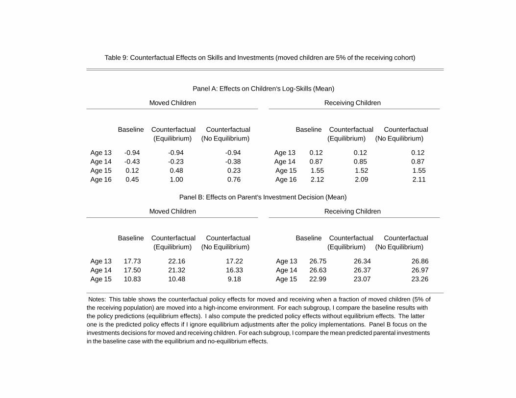
Table 9: Counterfactual Effects on Skills and Investments (moved children are 5% of the receiving cohort)

Panel A: Effects on Children‘s Log-Skills (Mean)

Moved Children Receiving Children

Baseline Counterfactual Counterfactual Baseline Counterfactual Counterfactual(Equilibrium) (No Equilibrium) (Equilibrium) (No Equilibrium)

Age 13 -0.94 -0.94 -0.94 Age 13 0.12 0.12 0.12Age 14 -0.43 -0.23 -0.38 Age 14 0.87 0.85 0.87Age 15 0.12 0.48 0.23 Age 15 1.55 1.52 1.55Age 16 0.45 1.00 0.76 Age 16 2.12 2.09 2.11

Panel B: Effects on Parent‘s Investment Decision (Mean)

Moved Children Receiving Children

Baseline Counterfactual Counterfactual Baseline Counterfactual Counterfactual(Equilibrium) (No Equilibrium) (Equilibrium) (No Equilibrium)

Age 13 17.73 22.16 17.22 Age 13 26.75 26.34 26.86Age 14 17.50 21.32 16.33 Age 14 26.63 26.37 26.97Age 15 10.83 10.48 9.18 Age 15 22.99 23.07 23.26

Notes: This table shows the counterfactual policy effects for moved and receiving when a fraction of moved children (5% ofthe receiving population) are moved into a high-income environment. For each subgroup, I compare the baseline results withthe policy predictions (equilibrium effects). I also compute the predicted policy effects without equilibrium effects. The latterone is the predicted policy effects if I ignore equilibrium adjustments after the policy implementations. Panel B focus on theinvestments decisions for moved and receiving children. For each subgroup, I compare the mean predicted parental investmentsin the baseline case with the equilibrium and no-equilibrium effects.

Table 10: Counterfactual Effects on Skills and Investments (moved children are 30% of the receiving cohort)

Panel A: Effects on Children‘s Log-Skills (Mean)

Moved Children Receiving Children Remained Children

Baseline Counterfactual Counterfactual Baseline Counterfactual Counterfactual Baseline Counterfactual Counterfactual(Equilibrium) (No Equilibrium) (Equilibrium) (No Equilibrium) (Equilibrium) (No Equilibrium)

Age 13 -1.00 -1.00 -1.00 Age 13 0.12 0.12 0.12 Age 13 -0.05 -0.05 -0.05Age 14 -0.37 -0.28 -0.33 Age 14 0.87 0.80 0.87 Age 14 0.42 0.52 0.43Age 15 0.24 0.40 0.34 Age 15 1.55 1.43 1.55 Age 15 0.87 1.05 0.88Age 16 0.53 0.84 0.80 Age 16 2.12 1.97 2.11 Age 16 1.26 1.49 1.29

Panel B: Effects on Parent‘s Investment Decision (Mean)

Moved Children Receiving Children Remained Children

Baseline Counterfactual Counterfactual Baseline Counterfactual Counterfactual Baseline Counterfactual Counterfactual(Equilibrium) (No Equilibrium) (Equilibrium) (No Equilibrium) (Equilibrium) (No Equilibrium)

Age 13 17.89 19.52 17.89 Age 13 26.75 24.74 27.22 Age 13 18.57 21.00 18.04Age 14 18.00 18.62 17.15 Age 14 26.63 24.84 27.72 Age 14 18.84 21.16 18.16Age 15 11.77 11.35 10.98 Age 15 22.99 22.82 23.92 Age 15 18.11 18.69 17.53

Notes: This table shows the counterfactual policy effects for moved and receiving when a fraction of moved children (30% of the receiving population) are moved into a high-income environment.For each subgroup, I compare the baseline results with the policy predictions (equilibrium effects). I also compute the predicted policy effects without equilibrium effects. The latter one is thepredicted policy effects if I ignore equilibrium adjustments after the policy implementations. Panel B focus on the investments decisions for moved, receiving and remained children. For eachsubgroup, I compare the mean predicted parental investments in the baseline case with the equilibrium and no-equilibrium effects.

Table 11: Counterfactual Effects on Receiving Children by Race (moved children are 30% of the receiving cohort)

Panel A: Effects on Children‘s Log-Skills (Mean)

Black Hispanic White

Baseline Counterfactual Baseline Counterfactual Baseline Counterfactual(Equilibrium) (Equilibrium) (Equilibrium)

Age 13 -0.30 -0.30 Age 13 -0.34 -0.34 Age 13 0.22 0.22Age 14 0.28 0.08 Age 14 0.45 0.30 Age 14 0.97 0.93Age 15 0.96 0.61 Age 15 1.08 0.81 Age 15 1.66 1.58Age 16 1.49 1.07 Age 16 1.59 1.24 Age 16 2.24 2.13

Panel B: Effects on Parent‘s Investment Decision (Mean)

Black Hispanic White

Baseline Counterfactual Baseline Counterfactual Baseline Counterfactual(Equilibrium) (Equilibrium) (Equilibrium)

Age 13 20.09 15.30 Age 13 21.97 17.72 Age 13 27.92 26.41Age 14 18.85 14.46 Age 14 20.67 16.62 Age 14 28.02 26.72Age 15 16.32 14.97 Age 15 16.69 14.99 Age 15 24.29 24.40

Notes: This table shows the counterfactual policy effects for receiving children (by race) when a fraction of moved children (30% of thereceiving population) are moved into a high-income environment. For each subgroup, I compare the baseline results in skills and parentalinvestments (Panel B) with the equilibrium counterfactual predictions.

Table 12: Counterfactual Effects on Skills and Investments of Earlier Interven-tions

Panel A: Effects on Children‘s Log-Skills (Mean)

Baseline Counterfactual Similar Children in Richer Environment

Age 13 -1.00 0.46 0.46Age 14 -0.37 0.85 1.09Age 15 0.24 1.31 1.74Age 16 0.53 1.73 2.31

Panel B: Effects on Parent‘s Investment Decision (Mean)

Baseline Counterfactual Similar Children in Richer Environment

Age 13 17.89 20.82 26.47Age 14 18.01 20.76 26.20Age 15 11.77 20.24 24.85

Notes: This table shows the counterfactual policy effects of fostering initial skills (age 13) inskill formation and parental investments (Panel B) for disadvantaged children. Column 1 and 2report the baseline and counterfactual predictions. Column 3 reports the dynamics of skills andparental investments for children with same mean initial skills at age 13 but who are living in thehigh-income environment.

64

Figure 1: Homophily in Network Formation by Race

Notes: This figure displays analysis on network formation using the homophily index (see Cole-man (1958)). In detail, letting fx,s be the average fraction of friends who are of the same race x atschool s and qx,s to be the total fraction of children of race x in a given school s, the homophily-

bias index looks as HB Ix,s = fx,sqx,s

.

65

Figure 2: Homophily in Network Formation by Skills

Notes: This figure displays analysis on network formation using the homophily index (see Coleman (1958)). In detail, letting fx,s

be the average fraction of friends who are of similar skills level x at school s and qx,s to be the total fraction of similar children with

skills level x in a given school s, the homophily-bias index looks as HB Ix,s = fx,sqx,s

.

Figure 3: First Stage Graphs

-.2-.1

0.1

.2Pe

ers'

Ski

lls

01

23

Den

sity

(%)

-1 -.5 0 .5 1Instrumental Variable (Z_1,i,t)

(a) First instrument: Fraction of Minority Children

-.2-.1

0.1

.2Pe

ers'

Ski

lls

0.5

11.

52

Den

sity

(%)

-1 -.5 0 .5 1Instrumental Variable (Z_2,i,t)

(b) Second instrument: Fraction of White Children

Notes: This figure shows graphically the first stage effects of the instrumental variables. Bothgraphs show the within-school variation of IV (x-axis) and the peers’ skills (y-axes). Solid linesrepresents a linear regression of peer’s skills on each of the two instrumental variables, aftercontrolling for school fixed effects and all the covariates in Table 2. Dashed lines show 90%confidence intervals. The plotted values on the background show the overall variation of bothinstrumental variables (top and bottom 1% excluded).

Figure 4: The Probability Two Children Become Friends by Skills and Race

(a) Low Skill (First Quartile) Black Children (b) Low Skill (First Quartile) White Children

This figure displays the probability that two children become friends by children skills and race. Figure (a) shows the marginalprobability for a black child with low skills (in the first quartile of skill distribution at age 14) to become friends with differentchildren over the spectrum of skills and for different races. Figure (b) shows the same graph but for a white child with low skills (inthe first quartile of skill distribution at age 14).

Figure 5: Model Validation from Exposure Effects in Children from Chetty and Hendren (2016a)

Notes: This figure displays the comparison between model’s predictions and findings in Chettyand Hendren (2016a) about childhood exposure effects.

69

Figure 6: Decomposition Exposure Effects for Disadvantaged Children

Notes: This figure displays the graphical decomposition for disadvantaged children of child-hood exposure effects by: peers, school and neighborhood quality.

70

Figure 7: Peers’ Skills Distribution (Baseline vs Counterfactual Economy)

Notes: This figure shows the equilibrium distribution of peers’ skills for moved and receiving children by age, before and after thepolicy is implemented. Parent’s expectations about future peers’ skills are based on the above distributions. The policy moved afraction of disadvantaged children into a high-income environment (approximately 30% of the population of the receiving cohort).

Figure 8: Treatment Effect by Skills (Moved-Receiving-Remained Children)

Notes: This figure shows the heterogeneous treatment effects on child’s age 16 skills by initial (age 13) child’s skills percentile formoved, receiving and remained children. The policy moved a fraction of disadvantaged children into a high-income environment(approximately 30% of the population of the receiving cohort).

Figure 9: Treatment Effect by Fraction of Moved Eligible Children (Moved-Receiving-Remained Children)

Notes: This figure shows the effect of the size of moved children for the policy returns for moved, receiving and remained children.Eligible children live in low-income environments and are below first quartile of age 13 skill distribution.

Figure 10: Peers’ Skills Distribution (Low-Income vs High-Income)

Notes: This figure shows the equilibrium distribution of peers’ skills for the children who received the initial boost of skills butstill live in the low-income environment and their similar counterpart living in high-income environment. Parent’s expectationsabout future peers’ skills are based on the above distributions.

A Data Appendix

The Add Health database was designed to study the impact of the social environment (i.e.

friends, family, neighborhood and school) on adolescents’ behavior in the United States of

America. Add Health’s original sample comprises students of 132 representative schools in the

United States. There are 90,118 students, ranging between grades 7 and 12 in the 1994–1995

school year (Wave I). A subsample of students (20,745) was selected for an additional home

interview (in-home). The home interview includes new questions for the children and a ques-

tionnaire for one of their parents. Information related to school quality and area of residence

makes the data set attractive. Those surveyed were interviewed again in 1995–96 (Wave II),

2001–2002 (Wave III), and 2007–2008 (Wave IV). The data set includes specific information on

family background, students’ school grades and their scores in the Add Health Picture Vocabu-

lary Test (AHPVT – a revised version of the Peabody Picture Vocabulary Test [PPVT]), as well as

information about children’s peers.

A main source of information which makes the Add Health data set particularly attractive for

achieving the objective of this project is the friendship nomination. During the first two waves,

children were asked, both during the in-home and in-school interviews, to nominate their best

five male and best five female friends. This detailed information helped me to reconstruct the

structure of friendship for every child in the sample by simply matching their identifier.

A.1 Measures for Children’s Skills and Parental Investments

The Peabody Picture Vocabulary Test (PPVT) was developed in 1959 as a test of receptive vocab-

ulary and is oriented to give an estimation of verbal ability and school aptitude. More generally,

it intends to provide a measure of intelligence. The test is age standardized, and performance

does not depend on the reading ability of the test-taker. The test-giver reads a word, and the

test-taker selects the image she thinks best fits the meaning of the word from among four simple

illustrations.

In the Add Health dataset, a computerized and shorter version of the Peabody Picture Vocab-

ulary Test, the AHPVT, has been implemented. The AHPVT includes half of the questions of

the original PPVT (every other item in the original sequence was selected for use). Add Health

provides two versions of the AHPVT: raw and standardized test scores. The standardized ver-

sion has a mean of 100 and a standard deviation of 15 and is standardized by age (for further

technical details about the AHPVT, see Halpern, 2000).

75

Add Health provides information about the AHPVT test scores for Waves I, III and IV. During

Wave I, respondents are between 11 and 21 years old. I consider this piece of information as one

of the measures of children’s latent skills. Additionally, I consider children’s grades at school for

both Wave I and Wave II. Analyzing all these multiple measurements, I am able to combine both

the cross-sectional as well as the longitudinal information about child development.

During the in-home interview in Wave I and Wave II, children provided information about

activities they had engaged in with their parents during the previous four weeks. These activit-

ies include: going shopping, sport activities, going to a movie/museum/concert or sport event,

talking about personal problems or school, or working on a project for school. There are a total

of nine activities each child can do with their parents. These types of activities provide inform-

ation about the level of parental engagement with their child. During Wave I, a parent, prefer-

ably the resident mother, of each adolescent respondent was interviewed (in-home interview).

The parent questionnaire included a question about the achieved level of education for the re-

spondent, which is considered as one proxy for the mother’s skills. During the same survey, the

respondent provided information about total family income during the previous calendar year.

76

B Additional Figures and Tables

Figure B-1: Probability of the Friendships and School’s Size

Notes: This figure shows the probability, for each school, that a child becomes friend with an-other child as function of school’s size.

77

Figure B-2: Mean of Children Skills by Race (Low-Income Neighborhood)

Notes: This figure shows the sample fit for the mean of children’s skills for low-quality (low-income) neighborhood by race.

Figure B-3: Mean of Children Skills by Race (Medium-Income Neighborhood)

Notes: This figure shows the sample fit for the mean of children’s skills for medium-quality (medium-income) neighborhood byrace.

Figure B-4: Mean of Children Skills by Race (High-Income Neighborhood)

Notes: This figure shows the sample fit for the mean of children’s skills for high-quality (high-income) neighborhood by race.

Figure B-5: Standard Deviation of Children Skills by Race (Low-Income Neighborhood)

Notes: This figure shows the sample fit for the standard deviation of children’s skills for low-quality (low-income) neighborhoodby race.

Figure B-6: Standard Deviation of Children Skills by Race (Medium-Income Neighborhood)

Notes: This figure shows the sample fit for the standard deviation of children’s skills for medium-quality (medium-income) neigh-borhood by race.

Figure B-7: Standard Deviation of Children Skills by Race (High-Income Neighborhood)

Notes: This figure shows the sample fit for the standard deviation of children’s skills for high-quality (high-income) neighborhoodby race.

Figure B-8: Index for Skills Homophily by Neighborhoods

Notes: This figure shows the sample fit for the homophily index for skills by by neighborhood-quality type (low-median-highincome).

Figure B-9: Index for Race Homophily by Neighborhoods

Notes: This figure shows the sample fit for the homophily index for race by by neighborhood-quality type (low-median-highincome).

Table B-1: Sample Statistics by Neighborhood Types

Neighborhood’s Type (1) (2) (3)

Panel A: Fraction of Families by Race

Fraction Black (%) 31.74 14.00 5.36

Fraction Hispanic (%) 26.77 14.50 10.86

Fraction White (%) 41.50 71.50 83.78

Panel B: Family Income (in 1994 $)

Mean Family Income

Family Income 29,637 43,458 57,512

Mean Family Income by Race

Black Family 26,917 41,778 46,592

Hispanic Family 26,167 33,749 49,940

White Family 34,046 45,632 59,224

Panel C: Children PPVT Achievements

Mean PPVT by Race

Black Children 57.02 62.37 64.39

Hispanic Children 58.06 60.33 64.51

White Children 63.87 66.46 69.98

PPVT Gaps between Neighborhoods

Black Children 66 (% SD) 18 (% SD) -

Hispanic Children 58 (% SD) 37 (% SD) -

White Children 55 (% SD) 32 (% SD) -

PPVT Gaps within Neighborhoods

Black Children 61 (% SD) 37 (% SD) 50(% SD)

Hispanic Children 52 (% SD) 55 (% SD) 49(% SD)

White Children - - -

Notes: This table reports descriptive statistics by by neighborhood-quality type (low-medium-high income).

Table B-2: Sample Fit for Auxiliary Coefficients (Investments)

Dependent Variable

Fraction (%) of Invested Parental Time

Measurement Error Adjusted Measurement Error Adjusted Measurement Error Adjusted Measurement Error Adjustedand and

Instrumental Variables (IV) Instrumental Variables (IV)

Data Model

Child Skills (Log) 2.660 2.120 2.152 3.124(0.316) (0.668)

[2.041,3.280] [0.810,3.430]

Peers’ Skills (Log) -1.441 0.720 -1.272 0.895(0.650) (0.354)

[-2.715,-0.167] [0.026,1.414]

First Stage First Stage

Z1,i ,t (Minorities Children) -0.104 -0.127(0.052)

[-0.206,-0.002]

Z2,i ,t (White Children) 0.082 0.105(0.037)

[0.009,0.155]

Notes: This table shows the sample fit for auxiliary regression coefficients for models in (2). Columns 1 and 2 shows the same estimated coefficients as in Table 2. Bothstandard errors in parenthesis and the 95% confidence interval in square brackets are computed using a cluster bootstrap.Data source: National Longitudinal Survey of Adolescent Health (Add Health).

Table B-3: Sample Fit for Auxiliary Coeffi-cients (Dynamics of Skills)

Data Model

Investments (Log) 0.408 0.343(0.197)

[0.021,0.794]

Child‘s Skills (Log) 0.750 0.760(0.238)

[0.283,1.216]

Peer‘s Skills (Log) 0.366 0.167(0.167)

[0.038,0.693]

Notes: This table shows the sample fit for auxiliaryregression coefficients of the auxiliary model for thedynamics of children’s skills. The dependent variableis the next period (t+1) child’s log-skills. The covari-ates in the table are: log-investments, current child’slog-skills, current peers’ log-skills. The regression alsoinclude as controls: age fixed effects, race, last periodfamily’s income, mother’s skills, school’s fixed effects.Both standard errors in parenthesis and the 95% con-fidence interval in square brackets are computed us-ing a cluster bootstrap.Data source: National Longitudinal Survey of Adoles-cent Health (Add Health).

88

Table B-4: Counterfactual Effects on Receiving Children by Race (moved children are 5% of the receiving cohort)

Panel A: Effects on Children‘s Log-Skills (Mean)

Black Hispanic White

Baseline Counterfactual Baseline Counterfactual Baseline Counterfactual(Equilibrium) (Equilibrium) (Equilibrium)

Age 13 -0.30 -0.30 Age 13 -0.34 -0.34 Age 13 0.22 0.22Age 14 0.28 0.23 Age 14 0.45 0.41 Age 14 0.97 0.96Age 15 0.96 0.87 Age 15 1.08 1.03 Age 15 1.66 1.64Age 16 1.49 1.39 Age 16 1.59 1.53 Age 16 2.24 2.21

Panel B: Effects on Parent‘s Investment Decision (Mean)

Black Hispanic White

Baseline Counterfactual Baseline Counterfactual Baseline Counterfactual(Equilibrium) (Equilibrium) (Equilibrium)

Age 13 20.09 19.01 Age 13 21.97 20.71 Age 13 27.92 27.67Age 14 18.85 17.94 Age 14 20.67 20.25 Age 14 28.02 27.85Age 15 16.32 16.36 Age 15 16.69 16.63 Age 15 24.29 24.37

Notes: This table shows the counterfactual policy effects for receiving children (by race) when a fraction of moved children (5% of the receivingpopulation) are moved into a high-income environment. For each subgroup, I compare the baseline results in skills and parental investments(Panel B) with the equilibrium counterfactual predictions.

C The Latent Factor Models

I consider the following latent factor model for either the child’s skills (hi ,t ) or the mother’s skills

(mi ):

Z hi ,t ,k =µh

t ,k +λht ,k · lnhi ,t +εh

i ,t ,k

Z mi ,k =µm

t ,k +λmk · lnmi +εm

i ,k (C-1)

where µs and λs are, respectively, the location and scale (or loading factor) parameters for each

considered measure k at any age t for each child i . The distribution of the latent factors is

identified by exploiting multiple measures in the data. One commonly used condition for iden-

tification is the independence of the joint distribution of latent variables and measurement

errors.

Assumption 1. Measurement model assumptions:

(i) εhi ,t ,k ⊥ εh

i ,t ,k ′ and εmi ,k ⊥ εm

i ,k ′ for all t and k 6= k ′

(ii) εhi ,t ,k ⊥ εh

i ,t ′,k ′ and εmi ,k ⊥ εm

i ,k ′ for all t 6= t ′ and all k and k ′

(iii) εhi ,t ,k ⊥ hi ,t ′ and εm

i ,k ⊥ mi for all t and t ′ and all k

(iv) εhi ,t ,k ⊥ εh

j ,t ,k and εmi ,k ⊥ εm

j ,k for all k and for any family j different from family i

(v) εhi ,t ,k , εm

i ,k ⊥ Xi , for all t and all k

Assumption 1 (i) is that measurement errors are independent contemporaneously across meas-

ures. Assumption 1 (ii) is that measurement errors are independent over time. Assumption 1

(iii) is that measurement errors in any period are independent of the latent variables in any

period. Assumption 1 (iv) that measurement errors are independent between observations. Fi-

nally, assumption 1 (v) assures that errors in measuring skills are independent of the observable

characteristics of children and mothers. While these assumptions are strong, they are common

in the current literature (see Cunha et al., 2010; Agostinelli and Wiswall, 2016). Assumptions

(i)–(v), together with the specification in (C-1), guarantee the non-parametric identification of

the latent distribution. However, in this work, I consider a parametric model of skill formation,

hence each of the conditions in (i)–(v) can be relaxed to statements about the zero correlation

between the considered variables, instead of the full independence conditions.

90

D Proof of Theorem 1

In this proof, I consider the two-period case. The four-period case follows by the induction hy-

pothesis. The proof is based on backward induction. The goal is to show that for each period

t , I can compute the policy functions for both parents and children that solve the fixed point

associated to the equilibrium conditions in (4.5). For the purpose of exposition, I employ only

the endogenous state variables of the problem (h, H) and define the technology of skill form-

ation in (4) as f (·).44 Finally, the proof is executed for the case of log utility (γ3 = γ5 = 1) and

perfect substitution between parents and peers (α4 = 1). This parametric case is the harder case

to prove an existence of a fixed point through Tarski’s fixed point theorem, and this is because

of the non-trivial preservation of monotonicity and supermodularity in the value function. Any

other case where either utility function is more convex or the technology provides higher com-

plementarity between endogenous inputs follows by construction. Hence, by proving that this

case admits a fixed point, I prove that a fixed point exists for any other admissible parameteriz-

ation of the model .

• Last period case (t = T ):

During the last period, children decide their own peer-solving problem (6) based on their

current level of skills. Parents observe the realization of their child’s network formation

and then make their last investment decision. No equilibrium conditions here are neces-

sary, since during the next period, no children’s network is formed. In other words, during

the last period, the equilibrium policy functions to solve the two (parent’s and child’s) de-

cision problems. The associated last period value function for parent i is:

V PT (hi ,T , H i ,T ) =

((τ− I∗T (hi ,T , H i ,T )

)·wi ,T + yi ,T

)γ1 + (γ2 +α1) log (hi ,T )

+βγ4log(α3I∗T (hi ,T , H i ,T )+ (1−α3)H i ,T

)(D-1)

Lemma 1. The value function V PT (hi ,T , H i ,T ) is monotone, increasing in both arguments

and supermodular.

Proof: It is easy to show that the policy function is monotone in both dimensions (monotone

increasing in the first argument and decreasing in the second argument). Hence, the value

44For clarity and without loss of generality, I ignore all the exogenous variables which are irrelevant for the equi-librium analysis, such as the mother’s skills and the family’s characteristics.

91

function clearly has monotone increasing in the first argument. Additionally, because of

the homothetic preferences, the overall peer effects H on children’s skills is positive, e.g.,

the change (decrease) of the policy function due to higher H does not dominate the initial

change in H.45 Hence, the value function is also increasing with the peer effects. To show

that the value is supermodular, consider the derivative of V PT with respect to hi ,T :

∂V PT (hi ,T , H i ,T )

∂hi ,T≡ γ2 +α1

hi ,T(D-2)

where equation (D-2) is derived applying the principle of optimality. Given equation (D-2)

is independent of Hi ,T , it follows trivially that V PT is supermodular in (hi ,T , H i ,T ).

• First period case (t = T −1):

In order to solve the parent’s problem and child’s problem differently (remember that par-

ents take a child’s decision regarding the next period’s network formation as a given), let

us define hi ,t+1 as the skills that children care about once they decide upon their friends

in the next period. Parents take hi ,t+1 as a given – that is, they think the process of the

formation of peer groups is independent of their investment decisions. In this case, the

parent’s problem is:

V PT−1(hi ,T−1, H i ,T−1 ; hi ,T ) =

maxIi ,T−1∈[0 ,τ]

((τ− Ii ,T−1

) ·wi ,T−1 + yi ,T−1)γ1 +γ2 hi ,T−1 +βE

[V P

T

(hi ,T

(Ii ,T−1

), H i ,T (hi ,T )

)∣∣∣hi ,T

](D-3)

where H i ,T (hi ,T ) is the stochastic mapping about the next period’s peer effects H i ,T given

hi ,T . Given the empirical evidence on children’s social interactions, I consider the case

when this mapping is stochastically ordered in hi ,T ,

E[

H i ,T (hi ,T )∣∣∣hi ,T

]≤ E

[H i ,T (hi ,T ’)

∣∣∣hi ,T ’]

if hi ,T < hi ,T ’,

which means that the higher the child’s skills, the higher the probability of becoming

friends with higher-skilled children. The fix-point problem here comes from the equi-

45This can be proved through the comparative statics of the problem, using the concavity of utility over con-sumption and children’s skills.

92

librium consistency conditions, which require that the endogenous network formation is

consistent with the parental decisions about the child’s development. In other words, in

the equilibrium path, I am imposing that the optimal level of children’s skills decided by

the parents are the same level of skills governing the network-formation decision

hi ,T = h∗i ,T .

To show that this fix point has a solution, I am applying standard results in the dynamic

lattice programming literature.

Lemma 2. Under Lemma 1, there exists a policy function IT−1(·) which solves the equilib-

rium fix-point problem in (D-3).

Proof: This result follows directly from Tarski’s fixed point theorem. The continuation value

is both increasing and supermodular in the two endogenous variables (individual endo-

genous children’s skills and peers’ skills). The stochastic process governing the network

formation stochastically ascends with respect to the children’s skills, and the choice set is

a complete lattice.

The Markovian equilibrium of the model is defined as the sequence of the policy func-

tions solves each of the two periods’ equilibrium problems.

93

E Indirect Inference

Part of the selected moments in the estimation procedure includes coefficients of auxiliary re-

gressions. In particular, I consider separate auxiliary models to analyze the parental investments

and the dynamics of skills. The first set of coefficients consider parental investments as the de-

pendent variable in the following linear regression

Ii ,s,t = β0 +β1 lnhi ,s,t +β2 ln H i ,s,t +X ′iβ3 +βs +ui ,s,t , (E-1)

where Ii ,s,t is the parental investment (as fraction of time) for parent of child i , in school s when

she is t years old, which is recovered through a latent factor model (see Section 5.1) using data

on parental engagement described in previous section. The child’s skills are defined as hi ,s,t

, while H i ,s,t is the mean of her peers’ skills. Xi is a vector of child and parents’ exogenous

characteristics, which includes race, age fixed-effects, lagged family income and mother’s skills.

Finally, βs is the school fixed effects. The coefficients of interests are related to how parental

investments respond to changes in child skills (β1) and peers’ skills (β2). In the estimation pro-

cedure, I include as targeted moments the parameters in (E-1), for both the school fixed-effects

estimator, as well as for the IV estimator explained in Section 3.4.

Additionally, I consider an auxiliary model of skill dynamics, where the next period skills are

the dependent variable of the following regression

lnhi ,s,t+1 = βh0 +βh

1 lnhi ,s,t +βh2 ln H i ,s,t +βh

3 ln Ii ,s,t +X ′iβ

h4 +βh

s +uhi ,s,t , (E-2)

where (βh0 ,βh

1 ,βh2 ,βh

3 ) are the specific auxiliary parameters I selected as targeting moments

for estimation. They represent respectively the elasticity of the next period skills with respect to

the stock of current skills, the peers’ skills and the parental investments. Xi is a vector of child

and parents’ exogenous characteristics, which includes race, age fixed-effects, lagged family

income and mother’s skills. Finally, βs is the school fixed effects. The estimated distribution of

school fixed-effects are used in the estimation as the school quality distributions in the model.

94