Investigations of Possible Low-Level Temperature and

DOE/SC-ARM/TR-119

Investigations of Possible Low-Level Temperature and Moisture Anomalies During the AMIE Field Campaign on Manus Island CN Long DJ Holdridge November 2012

DISCLAIMER

This report was prepared as an account of work sponsored by the U.S. Government. Neither the United States nor any agency thereof, nor any of their employees, makes any warranty, express or implied, or assumes any legal liability or responsibility for the accuracy, completeness, or usefulness of any information, apparatus, product, or process disclosed, or represents that its use would not infringe privately owned rights. Reference herein to any specific commercial product, process, or service by trade name, trademark, manufacturer, or otherwise, does not necessarily constitute or imply its endorsement, recommendation, or favoring by the U.S. Government or any agency thereof. The views and opinions of authors expressed herein do not necessarily state or reflect those of the U.S. Government or any agency thereof.

DOE/SC-ARM/TR-119

Investigations of Possible Low-Level Temperature and Moisture Anomalies During the AMIE Field Campaign on Manus Island CN Long DJ Holdridge November 2012

Work supported by the U.S. Department of Energy, Office of Science, Office of Biological and Environmental Research

CN Long and DJ Holdridge, November 2012, DOE/SC-ARM/TR-119

ii

Summary

This document discusses results stemming from the investigation of near-surface temperature and moisture “oddities” that were brought to light as part of the Atmospheric Radiation Measurement (ARM) Madden-Julian Oscillation (MJO) Investigation Experiment (AMIE), Dynamics of the Madden-Julian Oscillation (DYNAMO), and Cooperative Indian Ocean experiment on intraseasonal variability in the Year 2011 (CINDY2011) campaigns.

This report is submitted to document the extensive analyses of the Manus Island, Gan Island, and Nauru near-surface sonde data and corresponding manually entered data. A collaborative effort to produce the highest quality AMIE/DYNAMO/CINDY2011 sounding network data set is being led by Colorado State University (CSU) staff, who organized two workshops on February 6–7, 2012, and June 20, 2012. The analyses presented here were generated as a result of participation by the AMIE principal investigator in these workshops and extensive communications with other workshop attendees.

1. It was determined that the practice of using surface meteorological readings from the ARM Climate Research Facility’s forced air ventilated surface meteorological instrumentation (MET) system is preferable to using measurements from the Australian Automated Weather System (AWS) in a standard Stephenson enclosure with no forced air ventilation. As a result, ARM Operations switched to using MET measurements for the manually entered surface values for sonde launches in March 2012.

2. Use of the remote balloon launching (RBL) system, with the attendant long pipe used to supply forced air ventilation of the sonde package before launch, may be causing abnormally high temperatures on the sonde prior to launch during daylight hours.

3. At night, Manus exhibits persistent occurrence of shallow temperature inversions (45 meters on average), along with an increase in absolute humidity in the layer. This result remains after extensive study of factors that might artificially produce a similar result in sonde data that do not appear to have significant impact. The temperature inversions and absolute humidity profile are shown to make physical sense, particularly in relation to winds and haze/dew formation, and do also occur occasionally on Gan and Nauru under similar conditions.

4. It is recommended that ARM use surface MET data from forced air ventilated instruments and that the sondes themselves also be forced air ventilated prior to launch. Improvement in the Tropical Western Pacific site’s RBL design might be studied to mitigate the daylight sonde package heating prior to launch.


iii

Acronyms and Abbreviations

AMIE ARM MJO Investigation Experiment ARM Atmospheric Radiation Measurement (Climate Research Facility) AWS Automated Weather System CINDY Cooperative Indian Ocean experiment on intraseasonal variability dP change in P (pressure) dq change in q (specific humidity) dz change in z (height) DYNAMO Dynamics of the Madden-Julian Oscillation GTS Global Telecommunication System MET meteorological instrumentation MJO Madden-Julian Oscillation MRH manually entered RH (values) MT manually entered (values) NCAR National Center for Atmospheric Research P pressure PTU pressure, temperature, relative humidity PVC polyvinyl chloride q specific humidity RBL Remote Balloon Launching RH relative humidity RTD resistance temperature detector SMET surface meteorology SRH sonde RH values ST sonde (values) T temperature Tdpt dew point temperature Tdry air temperature UTC Universal Time Coordinates Z Zulu time zone z height


iv

Contents

Summary ....................................................................................................................................................... ii Acronyms and Abbreviations ...................................................................................................................... iii 1.0 Near-Surface Temperatures for Manus, Gan, and Nauru Sondes ......................................................... 1

1.1 Introduction .................................................................................................................................. 1 1.2 Background Information .............................................................................................................. 1 1.3 Analyses ....................................................................................................................................... 3 1.4 Summary .................................................................................................................................... 13

2.0 Investigations of Sonde Low-level Changes in Specific Humidity and Pressure for AMIE-Manus and AMIE-Gan .......................................................................................................................................... 13 2.1 Surface Differences .................................................................................................................... 14

2.1.1 Change in q with Height .................................................................................................. 19 2.2 Summary and Conclusions ......................................................................................................... 28

3.0 Acknowledgements ............................................................................................................................ 31 4.0 References .......................................................................................................................................... 31 Appendix A ............................................................................................................................................... A.1


v

Figures

Figure 1. RBL system at Manus. ................................................................................................................ 2 Figure 2. Gan sonde balloon cart system. .................................................................................................. 2 Figure 3. Example sonde profile showing the near-surface “dry bias” issue and illustrating the

various regions of data used to generate the temperature differences, as well as 5-mb and 10-mb linear fit slope calculations used in analyses. ........................................................... 4

Figure 4. Time series of near-surface sonde variables as described in the report text for Manus.............. 5 Figure 5. Similar to Figure 4, but for the Manus RBL testing experimental days. .................................... 6 Figure 6. Similar to Figure 4, but sorted by time of day (UTC) and with the slope results

magnified and referenced to the right-hand axis. ....................................................................... 7 Figure 7. Time series of calculated slopes and the elapsed time from launch to traverse the

lowest 5 and 10 mb of the profile. .............................................................................................. 8 Figure 8. Similar to Figure 6, but for the Gan sondes. ............................................................................... 9 Figure 9. Similar to Figure 6, but for the Nauru sondes. .......................................................................... 10 Figure 10. Relative frequency of STaDiff for the Manus (solid) and Gan (dashed) sites for

daylight (red) and nighttime (blue) periods. ............................................................................. 10 Figure 11. Relative frequency of STaSlp5 (blue) and STaSlp10 (red) for Manus for nighttime

(solid) and daytime (dashed) time periods. ............................................................................... 11 Figure 12. Relative frequency of STaSlp5 (blue) and STaSlp10 (red) for Gan for nighttime

(solid) and daytime (dashed) time periods. ............................................................................... 12 Figure 13. Relative frequency of STaSlp5 (blue) and STaSlp10 (red) for Manuru for nighttime

(solid) and daytime (dashed) time periods. ............................................................................... 12 Figure 14. Differences between manually entered values of air temperature (“MT”, red) and RH

(“MRH”, yellow) and the corresponding sonde measurements (ST and SRH) at launch time for sondes from Manus (top) and Gan (bottom). .............................................................. 15

Figure 15. Similar to Figure 14 top, with Manus March 2012 data which used the ARM meteorological instrumentation (MET) data as manually entered surface values for RH (black) and air temperature (light blue) differences highlighted. ....................................... 16

Figure 16. Differences between manually entered values of surface pressure (“Mprs”, blue) and calculated q (“Mq”, light blue) and the corresponding sonde measurements (Sprs and Sq) at launch time for sondes from Manus (top) and Gan (bottom) ......................................... 17

Figure 17. Similar to Figure 16 top, with Manus March 2012 q (black) and surface pressure (red) differences highlighted ............................................................................................................. 18

Figure 18. Comparison of the difference in manually entered T minus sonde surface-level T (X-axis) versus the manually entered RH minus the sonde surface-level RH (Y-axis) for Manus. ...................................................................................................................................... 19

Figure 19. Lowest 5 mb of sonde flight slope of fitted line using PTU file data and excluding the surface values for air temperature (blue) and RH (red) separated by time of day at Manus (top) and Gan (bottom) ................................................................................................. 21

Figure 20. Linear slope of temperature of the lowest 5 mb of sonde flight plotted versus 10-m wind speed at launch time for Manus (top) and Gan (bottom) ................................................. 22

Figure 21. Calculations of dq/dP by various means for Manus data .......................................................... 23


vi

Figure 22. GTSq_slp (black) simulates the original finite difference method using the manually entered surface and first significant level data for times when a low-level inversion is detected, sGTSq_slp (red) uses the sonde surface data (instead of manually entered surface data) in the finite difference calculation. ...................................................................... 24

Figure 23. Similar to Figure 21, but for Gan data, and with the sGTSq_slp (yellow) added similar to Figure 22 which uses the sonde surface data (instead of manually entered surface data) in the finite difference calculation simulating the GTS calculations. .............................. 25

Figure 24. Slope of linear fit to sonde data using sonde surface data up to a detected low-level inversion (q_invslp, brown) or to 960 mb (q_slp, blue); or starting with the second sonde point through a detected low-level inversion (q_invslp2, light blue) or to 960 mb (q_slp2, red) for Manus (top) and Gan (bottom). ........................................................ 26

Figure 25. Difference in slope of linear fit to sonde data, between when using surface data or not in the fitting, for the surface to inversion layer (red) and surface to 960 mb layer (blue) for Manus (top) and Gan (bottom). ........................................................................................... 27

Figure 26. Surface RH at sonde launch time from the manually entered values (blue) and the sonde surface measurements (red) for Manus (top) and Gan (bottom) .................................... 29

Figure A1. Pressure depth of the layer from the surface to 1000 mb (blue) and surface to top of detected low-level inversion when occurring (red) for Manus (top) and Gan (bottom). ........ A.2

Figure A2. Difference between the surface q value calculated from manually entered values and the q value calculated at the top of detected inversions for Manus (blue) and Gan (red) by time of day. ........................................................................................................................ A.3

Figure A3. AMF2 sonde launch and surface MET systems. .................................................................... A.4 Figure A4. Manus sonde remote balloon launch and AWS surface met systems. .................................... A.5

Tables

Table A1. Listing and description of the various dq/dP calculations used in this study. ........................ A.1


1

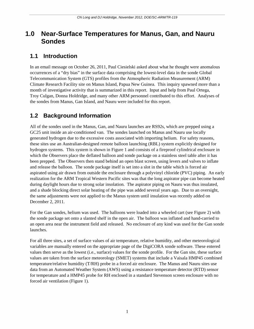
1.0 Near-Surface Temperatures for Manus, Gan, and Nauru Sondes

1.1 Introduction

In an email message on October 26, 2011, Paul Ciesielski asked about what he thought were anomalous occurrences of a “dry bias” in the surface data comprising the lowest-level data in the sonde Global Telecommunication System (GTS) profiles from the Atmospheric Radiation Measurement (ARM) Climate Research Facility site on Manus Island, Papua New Guinea. This inquiry spawned more than a month of investigative activity that is summarized in this report. Input and help from Paul Ortega, Troy Culgan, Donna Holdridge, and many other ARM personnel contributed to this effort. Analyses of the sondes from Manus, Gan Island, and Nauru were included for this report.

1.2 Background Information

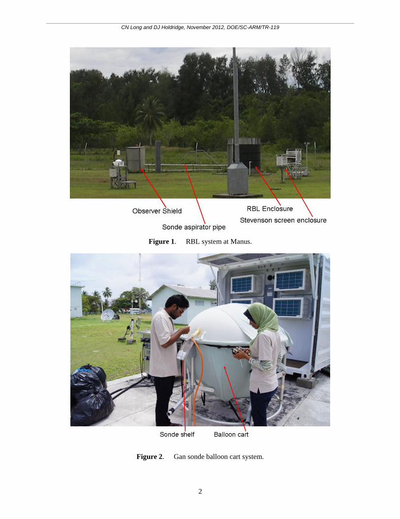
All of the sondes used in the Manus, Gan, and Nauru launches are RS92s, which are prepped using a GC25 unit inside an air-conditioned van. The sondes launched on Manus and Nauru use locally generated hydrogen due to the excessive costs associated with importing helium. For safety reasons, these sites use an Australian-designed remote balloon launching (RBL) system explicitly designed for hydrogen systems. This system is shown in Figure 1 and consists of a fireproof cylindrical enclosure in which the Observers place the deflated balloon and sonde package on a stainless steel table after it has been prepped. The Observers then stand behind an open blast screen, using levers and valves to inflate and release the balloon. The sonde package itself is set into a slot in the table which is forced air aspirated using air drawn from outside the enclosure through a polyvinyl chloride (PVC) piping. An early realization for the ARM Tropical Western Pacific sites was that the long aspirator pipe can become heated during daylight hours due to strong solar insolation. The aspirator piping on Nauru was thus insulated, and a shade blocking direct solar heating of the pipe was added several years ago. Due to an oversight, the same adjustments were not applied to the Manus system until insulation was recently added on December 2, 2011.

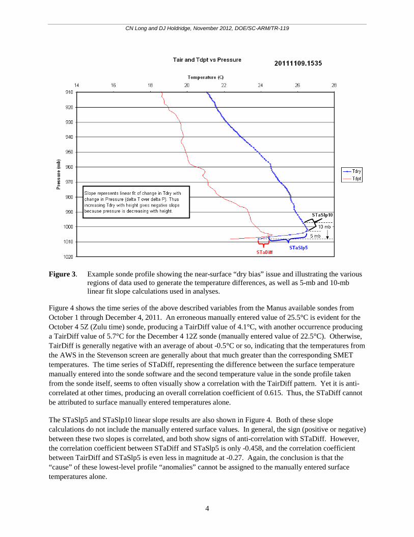
For the Gan sondes, helium was used. The balloons were loaded into a wheeled cart (see Figure 2) with the sonde package set onto a slanted shelf in the open air. The balloon was inflated and hand-carried to an open area near the instrument field and released. No enclosure of any kind was used for the Gan sonde launches.

For all three sites, a set of surface values of air temperature, relative humidity, and other meteorological variables are manually entered on the appropriate page of the DigiCORA sonde software. These entered values then serve as the lowest (i.e., surface) values for the sonde profile. For the Gan site, these surface values are taken from the surface meteorology (SMET) systems that include a Vaisala HMP45 combined temperature/relative humidity (T/RH) probe in a forced air enclosure. The Manus and Nauru sites use data from an Automated Weather System (AWS) using a resistance temperature detector (RTD) sensor for temperature and a HMP45 probe for RH enclosed in a standard Stevenson screen enclosure with no forced air ventilation (Figure 1).


2

Figure 1. RBL system at Manus.

Figure 2. Gan sonde balloon cart system.


3

1.3 Analyses

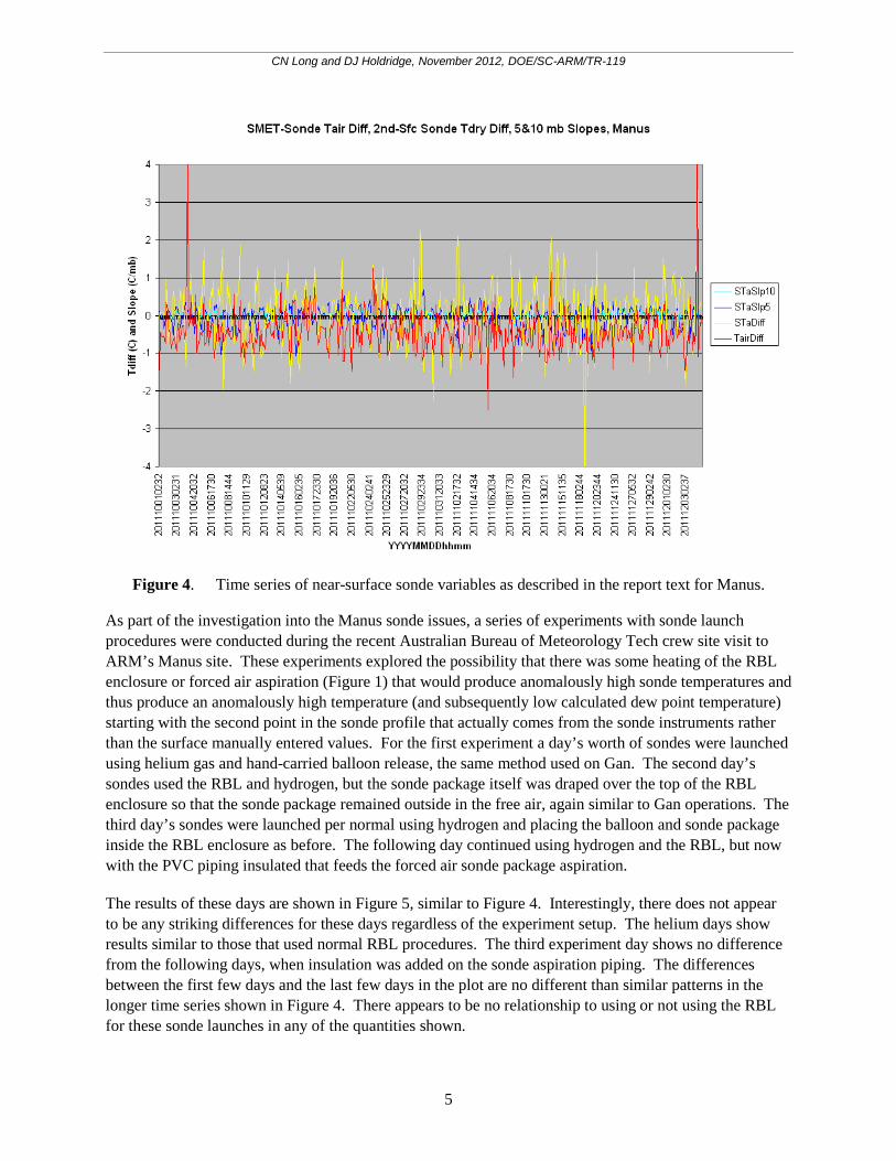
Figure 3 shows an illustration of the “dry bias” issue in the lowest part of a Manus sonde profile that Paul questioned. This plot and all the subsequent analyses use data from the high-resolution ARM netCDF sonde profile data (rather than the GTS messages) that include data at two-second intervals. In this case, the air temperature (Tdry) and dew point temperature (Tdpt) both show a rapid rise in value in the lowest 5 mb of ascent. Note that the manually entered surface variable for moisture is RH, not Tdry. The sonde itself also measures RH; it does not directly measure Tdpt. Thus, Tdpt is calculated using the variables Tdry and RH. A “low” Tdry value but a correct RH value will produce a “low” Tdpt value.

After viewing many of these lowest 100-mb sonde profiles from Gan, Manus, and Nauru, a convincing argument can be made that the “dry bias” issue that Paul has raised with the Manus sondes is not from the humidity measurements themselves, but rather in the calculation of dew point values and low air temperature measurements.

Also shown in Figure 3 are the various areas of the sonde data that are used in the subsequent plots. The variable “TairDiff” is not shown, but appears in subsequent plots. This variable is calculated by subtracting air temperature labeled as “Sounding Start Data” in the sonde “ptu” files (the manually entered temperature) from the measured air temperature from the respective site SMET system at the time of sonde launch (unfortunately the AWS system data for Manus and Nauru are not available to ARM). This variable serves to detect instances where the manually entered values might have been mistyped, causing large discrepancies, as well as (for the Manus and Nauru systems) the differences between forced air aspirated systems (SMET) and Stevenson screen enclosure systems plus an indication of instrument uncertainties.

The variable labeled “STaDiff” in Figure 3 is the difference between the lowest (surface) value in the sonde profile and the next higher in altitude value, calculated as the second minus the first. This serves to indicate the first value in these profiles from the sonde package instruments themselves versus the manually entered values represented in the first level values.

The variable “STaSlp5” represents the slope of a linear fit to the sonde data starting with the second height value (i.e., not including the manually entered first value) and including all data in the lowest 5 mb of the profile. The variable “STaSlp10” includes the data from 5 mb to the lowest 10 mb of the profile. These variables serve to illustrate the linear change in temperature with height in the initial 5 mb and 5–10 mb portions of the sonde flight. As noted in Figure 3, a negative slope indicates a tendency for an increase in temperature with height.


4

Figure 3. Example sonde profile showing the near-surface “dry bias” issue and illustrating the various

regions of data used to generate the temperature differences, as well as 5-mb and 10-mb linear fit slope calculations used in analyses.

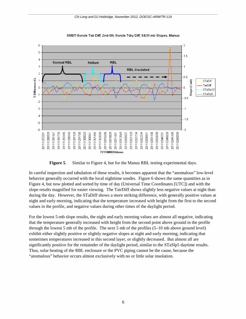
Figure 4 shows the time series of the above described variables from the Manus available sondes from October 1 through December 4, 2011. An erroneous manually entered value of 25.5°C is evident for the October 4 5Z (Zulu time) sonde, producing a TairDiff value of 4.1°C, with another occurrence producing a TairDiff value of 5.7°C for the December 4 12Z sonde (manually entered value of 22.5°C). Otherwise, TairDiff is generally negative with an average of about -0.5°C or so, indicating that the temperatures from the AWS in the Stevenson screen are generally about that much greater than the corresponding SMET temperatures. The time series of STaDiff, representing the difference between the surface temperature manually entered into the sonde software and the second temperature value in the sonde profile taken from the sonde itself, seems to often visually show a correlation with the TairDiff pattern. Yet it is anti-correlated at other times, producing an overall correlation coefficient of 0.615. Thus, the STaDiff cannot be attributed to surface manually entered temperatures alone.

The STaSlp5 and STaSlp10 linear slope results are also shown in Figure 4. Both of these slope calculations do not include the manually entered surface values. In general, the sign (positive or negative) between these two slopes is correlated, and both show signs of anti-correlation with STaDiff. However, the correlation coefficient between STaDiff and STaSlp5 is only -0.458, and the correlation coefficient between TairDiff and STaSlp5 is even less in magnitude at -0.27. Again, the conclusion is that the “cause” of these lowest-level profile “anomalies” cannot be assigned to the manually entered surface temperatures alone.


5

Figure 4. Time series of near-surface sonde variables as described in the report text for Manus.

As part of the investigation into the Manus sonde issues, a series of experiments with sonde launch procedures were conducted during the recent Australian Bureau of Meteorology Tech crew site visit to ARM’s Manus site. These experiments explored the possibility that there was some heating of the RBL enclosure or forced air aspiration (Figure 1) that would produce anomalously high sonde temperatures and thus produce an anomalously high temperature (and subsequently low calculated dew point temperature) starting with the second point in the sonde profile that actually comes from the sonde instruments rather than the surface manually entered values. For the first experiment a day’s worth of sondes were launched using helium gas and hand-carried balloon release, the same method used on Gan. The second day’s sondes used the RBL and hydrogen, but the sonde package itself was draped over the top of the RBL enclosure so that the sonde package remained outside in the free air, again similar to Gan operations. The third day’s sondes were launched per normal using hydrogen and placing the balloon and sonde package inside the RBL enclosure as before. The following day continued using hydrogen and the RBL, but now with the PVC piping insulated that feeds the forced air sonde package aspiration.

The results of these days are shown in Figure 5, similar to Figure 4. Interestingly, there does not appear to be any striking differences for these days regardless of the experiment setup. The helium days show results similar to those that used normal RBL procedures. The third experiment day shows no difference from the following days, when insulation was added on the sonde aspiration piping. The differences between the first few days and the last few days in the plot are no different than similar patterns in the longer time series shown in Figure 4. There appears to be no relationship to using or not using the RBL for these sonde launches in any of the quantities shown.


6

Figure 5. Similar to Figure 4, but for the Manus RBL testing experimental days.

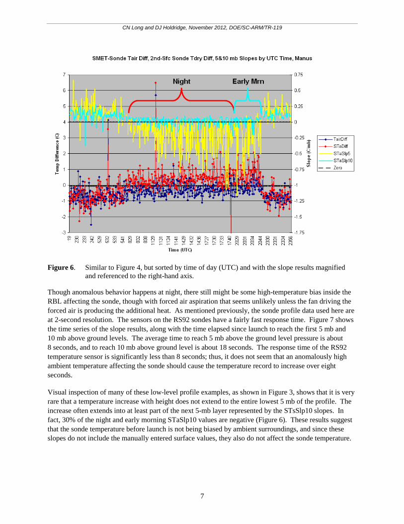
In careful inspection and tabulation of these results, it becomes apparent that the “anomalous” low-level behavior generally occurred with the local nighttime sondes. Figure 6 shows the same quantities as in Figure 4, but now plotted and sorted by time of day (Universal Time Coordinates [UTC]) and with the slope results magnified for easier viewing. The TairDiff shows slightly less negative values at night than during the day. However, the STaDiff shows a more striking difference, with generally positive values at night and early morning, indicating that the temperature increased with height from the first to the second values in the profile, and negative values during other times of the daylight period.

For the lowest 5-mb slope results, the night and early morning values are almost all negative, indicating that the temperature generally increased with height from the second point above ground in the profile through the lowest 5 mb of the profile. The next 5 mb of the profiles (5–10 mb above ground level) exhibit either slightly positive or slightly negative slopes at night and early morning, indicating that sometimes temperatures increased in this second layer, or slightly decreased. But almost all are significantly positive for the remainder of the daylight period, similar to the STaSlp5 daytime results. Thus, solar heating of the RBL enclosure or the PVC piping cannot be the cause, because the “anomalous” behavior occurs almost exclusively with no or little solar insolation.


7

Figure 6. Similar to Figure 4, but sorted by time of day (UTC) and with the slope results magnified

and referenced to the right-hand axis.

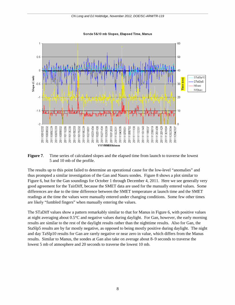
Though anomalous behavior happens at night, there still might be some high-temperature bias inside the RBL affecting the sonde, though with forced air aspiration that seems unlikely unless the fan driving the forced air is producing the additional heat. As mentioned previously, the sonde profile data used here are at 2-second resolution. The sensors on the RS92 sondes have a fairly fast response time. Figure 7 shows the time series of the slope results, along with the time elapsed since launch to reach the first 5 mb and 10 mb above ground levels. The average time to reach 5 mb above the ground level pressure is about 8 seconds, and to reach 10 mb above ground level is about 18 seconds. The response time of the RS92 temperature sensor is significantly less than 8 seconds; thus, it does not seem that an anomalously high ambient temperature affecting the sonde should cause the temperature record to increase over eight seconds.

Visual inspection of many of these low-level profile examples, as shown in Figure 3, shows that it is very rare that a temperature increase with height does not extend to the entire lowest 5 mb of the profile. The increase often extends into at least part of the next 5-mb layer represented by the STsSlp10 slopes. In fact, 30% of the night and early morning STaSlp10 values are negative (Figure 6). These results suggest that the sonde temperature before launch is not being biased by ambient surroundings, and since these slopes do not include the manually entered surface values, they also do not affect the sonde temperature.


8

Figure 7. Time series of calculated slopes and the elapsed time from launch to traverse the lowest

5 and 10 mb of the profile.

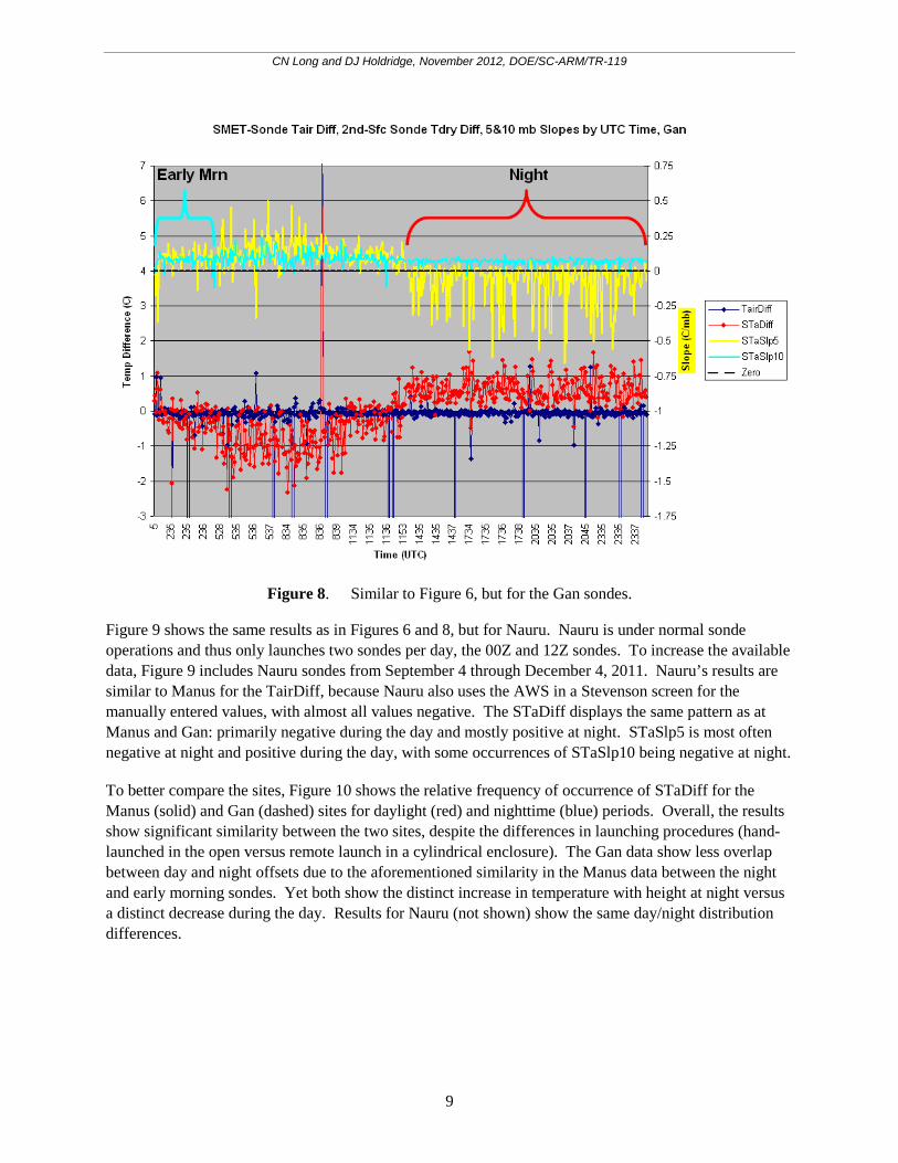
The results up to this point failed to determine an operational cause for the low-level “anomalies” and thus prompted a similar investigation of the Gan and Nauru sondes. Figure 8 shows a plot similar to Figure 6, but for the Gan soundings for October 1 through December 4, 2011. Here we see generally very good agreement for the TairDiff, because the SMET data are used for the manually entered values. Some differences are due to the time difference between the SMET temperature at launch time and the SMET readings at the time the values were manually entered under changing conditions. Some few other times are likely “fumbled fingers” when manually entering the values.

The STaDiff values show a pattern remarkably similar to that for Manus in Figure 6, with positive values at night averaging about 0.5°C and negative values during daylight. For Gan, however, the early morning results are similar to the rest of the daylight results rather than the nighttime results. Also for Gan, the StaSlp5 results are by far mostly negative, as opposed to being mostly positive during daylight. The night and day TaSlp10 results for Gan are rarely negative or near zero in value, which differs from the Manus results. Similar to Manus, the sondes at Gan also take on average about 8–9 seconds to traverse the lowest 5 mb of atmosphere and 20 seconds to traverse the lowest 10 mb.


9

Figure 8. Similar to Figure 6, but for the Gan sondes.

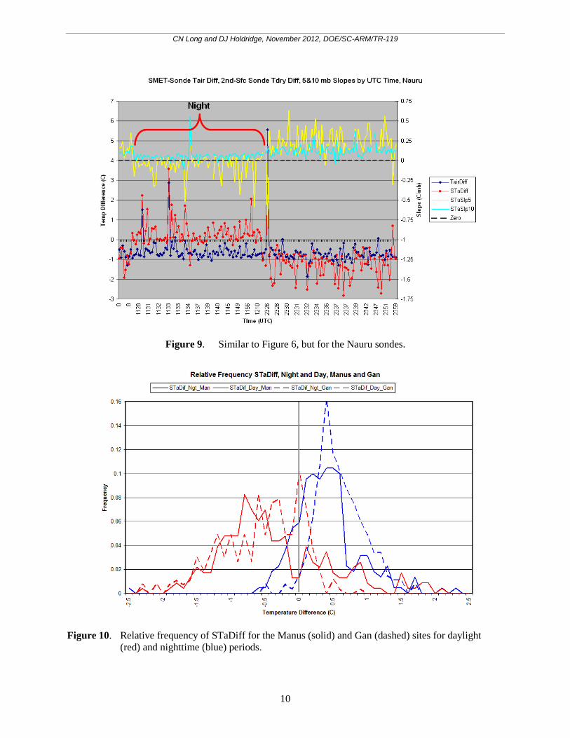
Figure 9 shows the same results as in Figures 6 and 8, but for Nauru. Nauru is under normal sonde operations and thus only launches two sondes per day, the 00Z and 12Z sondes. To increase the available data, Figure 9 includes Nauru sondes from September 4 through December 4, 2011. Nauru’s results are similar to Manus for the TairDiff, because Nauru also uses the AWS in a Stevenson screen for the manually entered values, with almost all values negative. The STaDiff displays the same pattern as at Manus and Gan: primarily negative during the day and mostly positive at night. STaSlp5 is most often negative at night and positive during the day, with some occurrences of STaSlp10 being negative at night.

To better compare the sites, Figure 10 shows the relative frequency of occurrence of STaDiff for the Manus (solid) and Gan (dashed) sites for daylight (red) and nighttime (blue) periods. Overall, the results show significant similarity between the two sites, despite the differences in launching procedures (hand-launched in the open versus remote launch in a cylindrical enclosure). The Gan data show less overlap between day and night offsets due to the aforementioned similarity in the Manus data between the night and early morning sondes. Yet both show the distinct increase in temperature with height at night versus a distinct decrease during the day. Results for Nauru (not shown) show the same day/night distribution differences.


10

Figure 9. Similar to Figure 6, but for the Nauru sondes.

Figure 10. Relative frequency of STaDiff for the Manus (solid) and Gan (dashed) sites for daylight

(red) and nighttime (blue) periods.


11

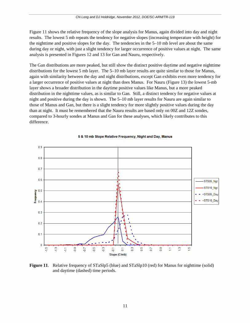
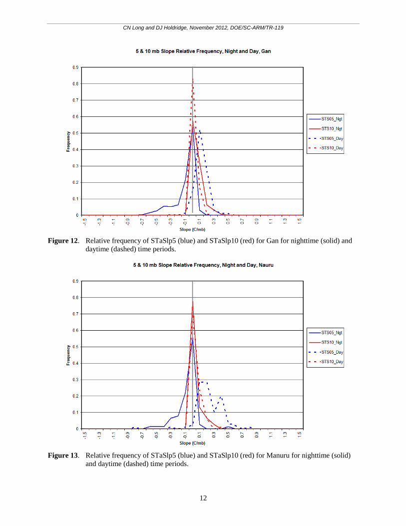
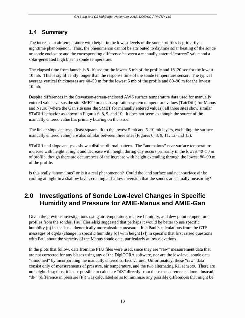
Figure 11 shows the relative frequency of the slope analysis for Manus, again divided into day and night results. The lowest 5 mb repeats the tendency for negative slopes (increasing temperature with height) for the nighttime and positive slopes for the day. The tendencies in the 5–10 mb level are about the same during day or night, with just a slight tendency for larger occurrence of positive values at night. The same analysis is presented in Figures 12 and 13 for Gan and Nauru, respectively.

The Gan distributions are more peaked, but still show the distinct positive daytime and negative nighttime distributions for the lowest 5 mb layer. The 5–10 mb layer results are quite similar to those for Manus, again with similarity between the day and night distributions, except Gan exhibits even more tendency for a larger occurrence of positive values at night than does Manus. For Nauru (Figure 13) the lowest 5-mb layer shows a broader distribution in the daytime positive values like Manus, but a more peaked distribution in the nighttime values, as is similar to Gan. Still, a distinct tendency for negative values at night and positive during the day is shown. The 5–10 mb layer results for Nauru are again similar to those of Manus and Gan, but there is a slight tendency for more slightly positive values during the day than at night. It must be remembered that the Nauru results are based only on 00Z and 12Z sondes, compared to 3-hourly sondes at Manus and Gan for these analyses, which likely contributes to this difference.

Figure 11. Relative frequency of STaSlp5 (blue) and STaSlp10 (red) for Manus for nighttime (solid)

and daytime (dashed) time periods.


12

Figure 12. Relative frequency of STaSlp5 (blue) and STaSlp10 (red) for Gan for nighttime (solid) and

daytime (dashed) time periods.

Figure 13. Relative frequency of STaSlp5 (blue) and STaSlp10 (red) for Manuru for nighttime (solid)

and daytime (dashed) time periods.


13

1.4 Summary

The increase in air temperature with height in the lowest levels of the sonde profiles is primarily a nighttime phenomenon. Thus, the phenomenon cannot be attributed to daytime solar heating of the sonde or sonde enclosure and the corresponding difference between a manually entered “correct” value and a solar-generated high bias in sonde temperature.

The elapsed time from launch is 8–10 sec for the lowest 5 mb of the profile and 18–20 sec for the lowest 10 mb. This is significantly longer than the response time of the sonde temperature sensor. The typical average vertical thicknesses are 40–50 m for the lowest 5 mb of the profile and 80–90 m for the lowest 10 mb.

Despite differences in the Stevenson-screen-enclosed AWS surface temperature data used for manually entered values versus the site SMET forced air aspiration system temperature values (TairDiff) for Manus and Nauru (where the Gan site uses the SMET for manually entered values), all three sites show similar STaDiff behavior as shown in Figures 6, 8, 9, and 10. It does not seem as though the source of the manually entered value has primary bearing on the issue.

The linear slope analyses (least squares fit to the lowest 5 mb and 5–10 mb layers, excluding the surface manually entered value) are also similar between three sites (Figures 6, 8, 9, 11, 12, and 13).

STaDiff and slope analyses show a distinct diurnal pattern. The “anomalous” near-surface temperature increase with height at night and decrease with height during day occurs primarily in the lowest 40–50 m of profile, though there are occurrences of the increase with height extending through the lowest 80–90 m of the profile.

Is this really “anomalous” or is it a real phenomenon? Could the land surface and near-surface air be cooling at night in a shallow layer, creating a shallow inversion that the sondes are actually measuring?

2.0 Investigations of Sonde Low-level Changes in Specific Humidity and Pressure for AMIE-Manus and AMIE-Gan

Given the previous investigations using air temperature, relative humidity, and dew point temperature profiles from the sondes, Paul Ciesielski suggested that perhaps it would be better to use specific humidity (q) instead as a theoretically more absolute measure. It is Paul’s calculations from the GTS messages of dq/dz (change in specific humidity [q] with height [z]) in specific that first raised questions with Paul about the veracity of the Manus sonde data, particularly at low elevations.

In the plots that follow, data from the PTU files were used, since they are “raw” measurement data that are not corrected for any biases using any of the DigiCORA software, nor are the low-level sonde data “smoothed” by incorporating the manually entered surface values. Unfortunately, these “raw” data consist only of measurements of pressure, air temperature, and the two alternating RH sensors. There are no height data; thus, it is not possible to calculate “dZ” directly from these measurements alone. Instead, “dP” (difference in pressure [P]) was calculated so as to minimize any possible differences that might be


14

introduced by any particular formulation in the conversion from pressure coordinates to height coordinates. Nonetheless, the various permutations of “dq/dP” are directly comparable.

Finally, also to minimize differences with Paul's previous calculations, Paul supplied his formulation to calculate “q” using the P, T, and RH data in the raw PTU files.

2.1 Surface Differences

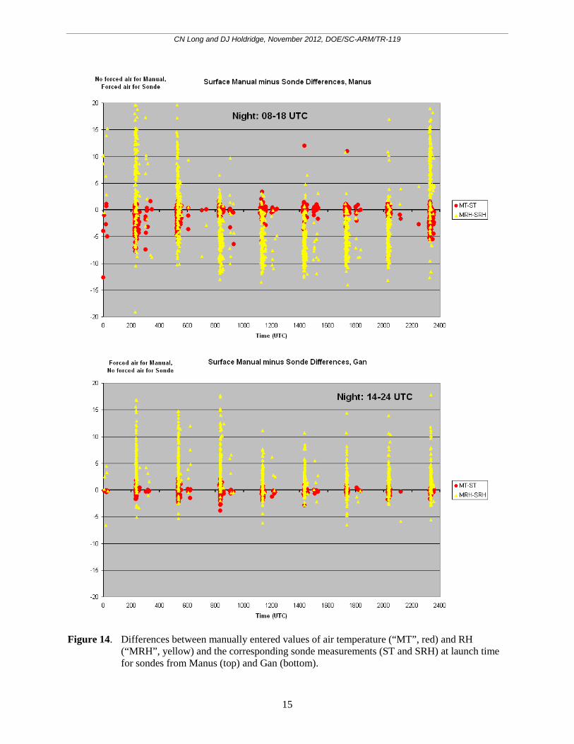
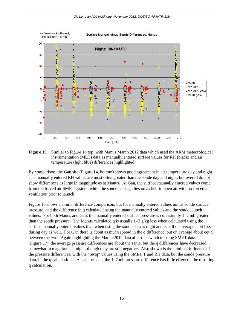
One possible source of anomalous dq results is the use of the manually entered surface data. As previously reported, comparisons do indicate some differences, particularly with the Manus data. Figure 14 (top) is similar to previous plots, but displays the complete AMIE-Manus 6-month data set plotted by UTC time. As noted before, the manually entered RH values (MRH) are usually less than the sonde RH values (SRH) at night, but most often the opposite during daylight hours. Air temperatures usually agree at night, but with manually entered values (MT) often a bit smaller than the sonde values (ST) during the day. For most of the AMIE-Manus deployment, surface manually entered values were taken from the Australian AWS system, with the sensors located in a standard non-forced air Stevenson screen enclosure, while the sonde package resides in a forced air flow drawn from outside the launch enclosure prior to launch. A switch was made later in the AMIE-Manus period to using surface manually entered values from the forced air ventilated SMET system. Figure 15 shows a plot similar to Figure 14 for Manus, but with the March 2012 data using forced air denoted for RH and Tair differences highlighted. The March data show some slight improvement in agreement for day and night Tair and night RH, but generally a more distinct pattern of manually entered RH being mostly greater than sonde during the day.


15

Figure 14. Differences between manually entered values of air temperature (“MT”, red) and RH

(“MRH”, yellow) and the corresponding sonde measurements (ST and SRH) at launch time for sondes from Manus (top) and Gan (bottom).


16

Figure 15. Similar to Figure 14 top, with Manus March 2012 data which used the ARM meteorological

instrumentation (MET) data as manually entered surface values for RH (black) and air temperature (light blue) differences highlighted.

By comparison, the Gan site (Figure 14, bottom) shows good agreement in air temperature day and night. The manually entered RH values are most often greater than the sonde day and night, but overall do not show differences as large in magnitude as at Manus. At Gan, the surface manually entered values come from the forced air SMET system, while the sonde package lies on a shelf in open air with no forced air ventilation prior to launch.

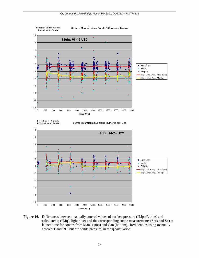
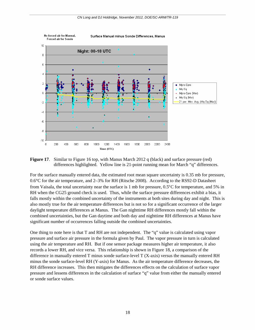
Figure 16 shows a similar difference comparison, but for manually entered values minus sonde surface pressure, and the difference in q calculated using the manually entered values and the sonde launch values. For both Manus and Gan, the manually entered surface pressure is consistently 1–2 mb greater than the sonde pressure. The Manus calculated q is usually 1–2 g/kg less when calculated using the surface manually entered values than when using the sonde data at night and is still on average a bit less during day as well. For Gan there is about as much spread in the q difference, but on average about equal between the two. Again highlighting the March 2012 data after the switch to using SMET data (Figure 17), the average pressure differences are about the same, but the q differences have decreased somewhat in magnitude at night, though they are still negative. Also shown is the minimal influence of the pressure differences, with the “SMq” values using the SMET T and RH data, but the sonde pressure data, in the q calculations. As can be seen, the 1–2 mb pressure difference has little effect on the resulting q calculation.


17

Figure 16. Differences between manually entered values of surface pressure (“Mprs”, blue) and

calculated q (“Mq”, light blue) and the corresponding sonde measurements (Sprs and Sq) at launch time for sondes from Manus (top) and Gan (bottom). Red denotes using manually entered T and RH, but the sonde pressure, in the q calculation.


18

Figure 17. Similar to Figure 16 top, with Manus March 2012 q (black) and surface pressure (red)

differences highlighted. Yellow line is 21-point running mean for March “q” differences.

For the surface manually entered data, the estimated root mean square uncertainty is 0.35 mb for pressure, 0.6°C for the air temperature, and 2–3% for RH (Ritsche 2008). According to the RS92-D Datasheet from Vaisala, the total uncertainty near the surface is 1 mb for pressure, 0.5°C for temperature, and 5% in RH when the CG25 ground check is used. Thus, while the surface pressure differences exhibit a bias, it falls mostly within the combined uncertainty of the instruments at both sites during day and night. This is also mostly true for the air temperature differences but is not so for a significant occurrence of the larger daylight temperature differences at Manus. The Gan nighttime RH differences mostly fall within the combined uncertainties, but the Gan daytime and both day and nighttime RH differences at Manus have significant number of occurrences falling outside the combined uncertainties.

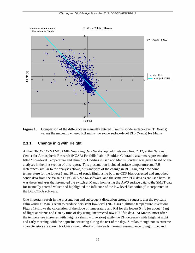
One thing to note here is that T and RH are not independent. The “q” value is calculated using vapor pressure and surface air pressure in the formula given by Paul. The vapor pressure in turn is calculated using the air temperature and RH. But if one sensor package measures higher air temperature, it also records a lower RH, and vice versa. This relationship is shown in Figure 18, a comparison of the difference in manually entered T minus sonde surface-level T (X-axis) versus the manually entered RH minus the sonde surface-level RH (Y-axis) for Manus. As the air temperature difference decreases, the RH difference increases. This then mitigates the differences effects on the calculation of surface vapor pressure and lessens differences in the calculation of surface “q” value from either the manually entered or sonde surface values.


19

Figure 18. Comparison of the difference in manually entered T minus sonde surface-level T (X-axis)

versus the manually entered RH minus the sonde surface-level RH (Y-axis) for Manus.

2.1.1 Change in q with Height

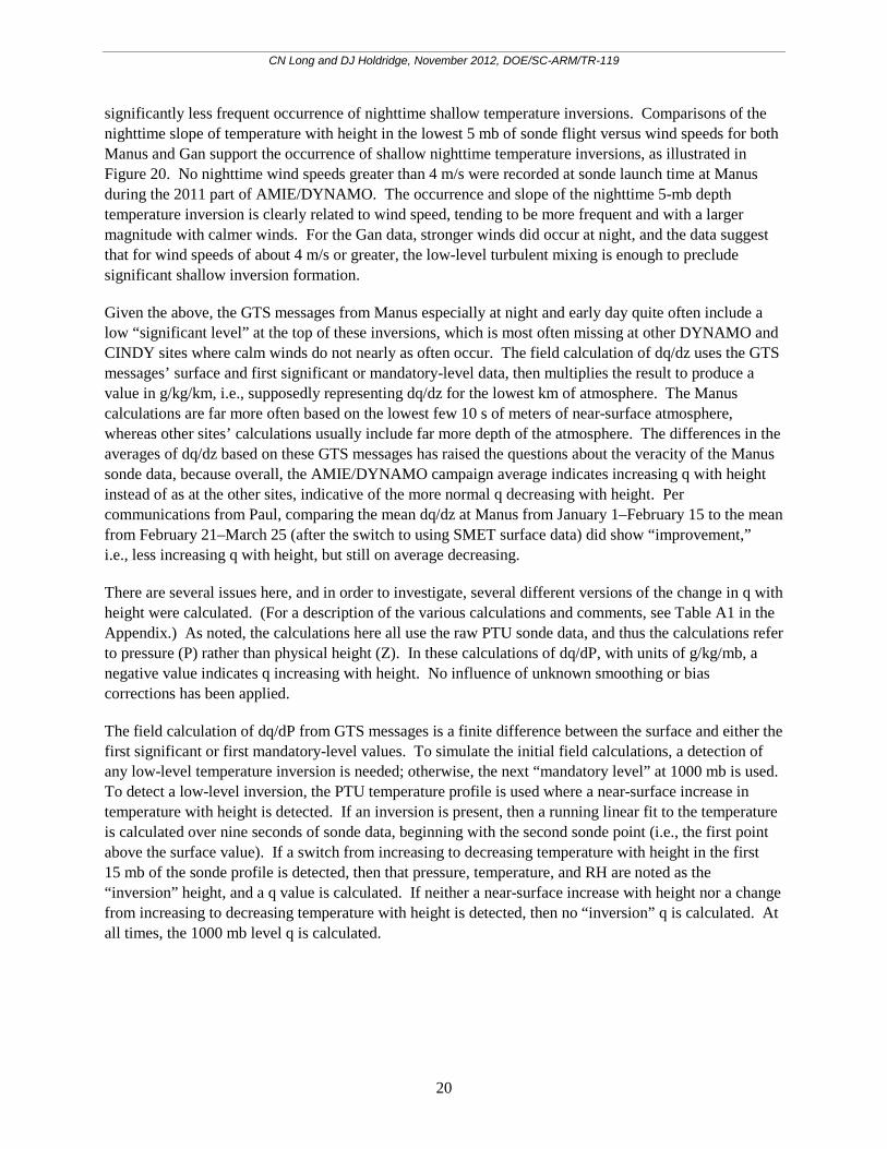
At the CINDY/DYNAMO/AMIE Sounding Data Workshop held February 6–7, 2012, at the National Center for Atmospheric Research (NCAR) Foothills Lab in Boulder, Colorado, a summary presentation titled “Low-level Temperature and Humidity Oddities in Gan and Manus Sondes” was given based on the analyses in the first section of this report. This presentation included surface temperature and RH differences similar to the analyses above, plus analyses of the change in RH, Tair, and dew point temperature for the lowest 5 and 10 mb of sonde flight using both netCDF bias-corrected and smoothed sonde data from the Vaisala DigiCORA V3.64 software, and the same raw PTU data as are used here. It was these analyses that prompted the switch at Manus from using the AWS surface data to the SMET data for manually entered values and highlighted the influence of the low-level “smoothing” incorporated in the DigiCORA software.

One important result in the presentation and subsequent discussion strongly suggests that the typically calm winds at Manus seem to produce persistent low-level (20–50 m) nighttime temperature inversions. Figure 19 shows the calculation of the slope of temperature and RH for the lowest 5 mb (or about 45 m) of flight at Manus and Gan by time of day using uncorrected raw PTU file data. At Manus, most often the temperature increases with height (a shallow inversion) while the RH decreases with height at night and early morning, with the opposite occurring during the rest of the day. Similar, though not as extreme characteristics are shown for Gan as well, albeit with no early morning resemblance to nighttime, and


20

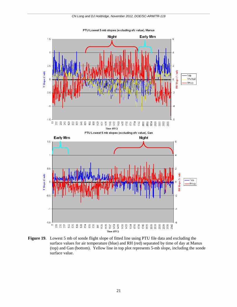
significantly less frequent occurrence of nighttime shallow temperature inversions. Comparisons of the nighttime slope of temperature with height in the lowest 5 mb of sonde flight versus wind speeds for both Manus and Gan support the occurrence of shallow nighttime temperature inversions, as illustrated in Figure 20. No nighttime wind speeds greater than 4 m/s were recorded at sonde launch time at Manus during the 2011 part of AMIE/DYNAMO. The occurrence and slope of the nighttime 5-mb depth temperature inversion is clearly related to wind speed, tending to be more frequent and with a larger magnitude with calmer winds. For the Gan data, stronger winds did occur at night, and the data suggest that for wind speeds of about 4 m/s or greater, the low-level turbulent mixing is enough to preclude significant shallow inversion formation.

Given the above, the GTS messages from Manus especially at night and early day quite often include a low “significant level” at the top of these inversions, which is most often missing at other DYNAMO and CINDY sites where calm winds do not nearly as often occur. The field calculation of dq/dz uses the GTS messages’ surface and first significant or mandatory-level data, then multiplies the result to produce a value in g/kg/km, i.e., supposedly representing dq/dz for the lowest km of atmosphere. The Manus calculations are far more often based on the lowest few 10 s of meters of near-surface atmosphere, whereas other sites’ calculations usually include far more depth of the atmosphere. The differences in the averages of dq/dz based on these GTS messages has raised the questions about the veracity of the Manus sonde data, because overall, the AMIE/DYNAMO campaign average indicates increasing q with height instead of as at the other sites, indicative of the more normal q decreasing with height. Per communications from Paul, comparing the mean dq/dz at Manus from January 1–February 15 to the mean from February 21–March 25 (after the switch to using SMET surface data) did show “improvement,” i.e., less increasing q with height, but still on average decreasing.

There are several issues here, and in order to investigate, several different versions of the change in q with height were calculated. (For a description of the various calculations and comments, see Table A1 in the Appendix.) As noted, the calculations here all use the raw PTU sonde data, and thus the calculations refer to pressure (P) rather than physical height (Z). In these calculations of dq/dP, with units of g/kg/mb, a negative value indicates q increasing with height. No influence of unknown smoothing or bias corrections has been applied.

The field calculation of dq/dP from GTS messages is a finite difference between the surface and either the first significant or first mandatory-level values. To simulate the initial field calculations, a detection of any low-level temperature inversion is needed; otherwise, the next “mandatory level” at 1000 mb is used. To detect a low-level inversion, the PTU temperature profile is used where a near-surface increase in temperature with height is detected. If an inversion is present, then a running linear fit to the temperature is calculated over nine seconds of sonde data, beginning with the second sonde point (i.e., the first point above the surface value). If a switch from increasing to decreasing temperature with height in the first 15 mb of the sonde profile is detected, then that pressure, temperature, and RH are noted as the “inversion” height, and a q value is calculated. If neither a near-surface increase with height nor a change from increasing to decreasing temperature with height is detected, then no “inversion” q is calculated. At all times, the 1000 mb level q is calculated.


21

Figure 19. Lowest 5 mb of sonde flight slope of fitted line using PTU file data and excluding the

surface values for air temperature (blue) and RH (red) separated by time of day at Manus (top) and Gan (bottom). Yellow line in top plot represents 5-mb slope, including the sonde surface value.


22

Figure 20. Linear slope of temperature of the lowest 5 mb of sonde flight plotted versus 10-m wind

speed at launch time for Manus (top) and Gan (bottom). Note the x-axis scale differences between the top and bottom plots.

Figure 21 shows the calculations of finite differences similar to the GTS calculations when an inversion occurs using the surface manually entered value and the value at the detected inversion top (GTSq_slp, black), plus a finite difference using the surface manually entered value and an average of the 2nd sonde data point up through 1000 mb data (1000AvSlp, light blue). Also, the linear slope of the line through the 2nd through 1000 mb data is shown (1000slp, red). As noted, most of the nighttime finite differences


23

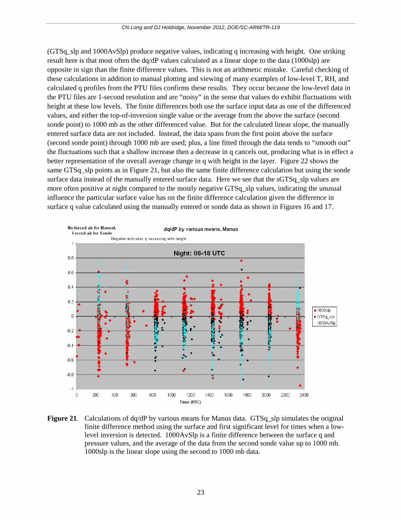
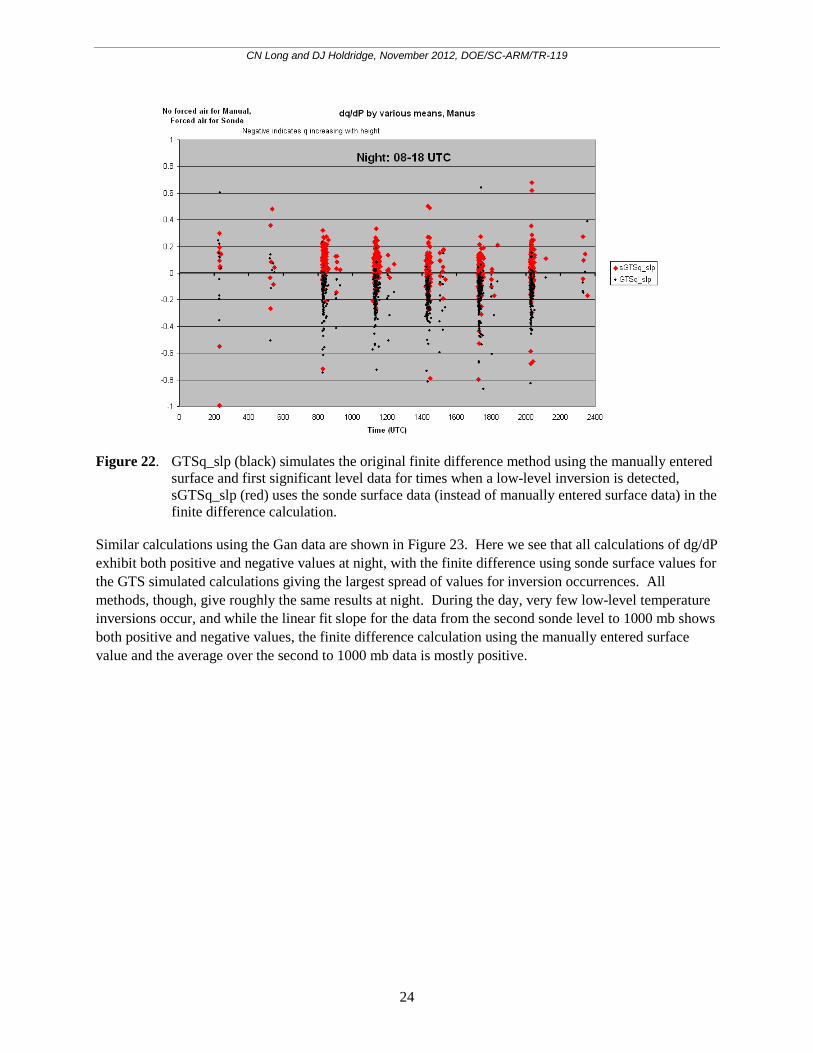
(GTSq_slp and 1000AvSlp) produce negative values, indicating q increasing with height. One striking result here is that most often the dq/dP values calculated as a linear slope to the data (1000slp) are opposite in sign than the finite difference values. This is not an arithmetic mistake. Careful checking of these calculations in addition to manual plotting and viewing of many examples of low-level T, RH, and calculated q profiles from the PTU files confirms these results. They occur because the low-level data in the PTU files are 1-second resolution and are “noisy” in the sense that values do exhibit fluctuations with height at these low levels. The finite differences both use the surface input data as one of the differenced values, and either the top-of-inversion single value or the average from the above the surface (second sonde point) to 1000 mb as the other differenced value. But for the calculated linear slope, the manually entered surface data are not included. Instead, the data spans from the first point above the surface (second sonde point) through 1000 mb are used; plus, a line fitted through the data tends to “smooth out” the fluctuations such that a shallow increase then a decrease in q cancels out, producing what is in effect a better representation of the overall average change in q with height in the layer. Figure 22 shows the same GTSq_slp points as in Figure 21, but also the same finite difference calculation but using the sonde surface data instead of the manually entered surface data. Here we see that the sGTSq_slp values are more often positive at night compared to the mostly negative GTSq_slp values, indicating the unusual influence the particular surface value has on the finite difference calculation given the difference in surface q value calculated using the manually entered or sonde data as shown in Figures 16 and 17.

Figure 21. Calculations of dq/dP by various means for Manus data. GTSq_slp simulates the original

finite difference method using the surface and first significant level for times when a low-level inversion is detected. 1000AvSlp is a finite difference between the surface q and pressure values, and the average of the data from the second sonde value up to 1000 mb. 1000slp is the linear slope using the second to 1000 mb data.


24

Figure 22. GTSq_slp (black) simulates the original finite difference method using the manually entered

surface and first significant level data for times when a low-level inversion is detected, sGTSq_slp (red) uses the sonde surface data (instead of manually entered surface data) in the finite difference calculation.

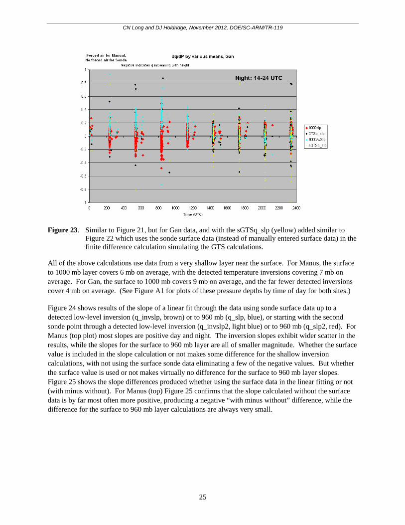
Similar calculations using the Gan data are shown in Figure 23. Here we see that all calculations of dg/dP exhibit both positive and negative values at night, with the finite difference using sonde surface values for the GTS simulated calculations giving the largest spread of values for inversion occurrences. All methods, though, give roughly the same results at night. During the day, very few low-level temperature inversions occur, and while the linear fit slope for the data from the second sonde level to 1000 mb shows both positive and negative values, the finite difference calculation using the manually entered surface value and the average over the second to 1000 mb data is mostly positive.


25

Figure 23. Similar to Figure 21, but for Gan data, and with the sGTSq_slp (yellow) added similar to

Figure 22 which uses the sonde surface data (instead of manually entered surface data) in the finite difference calculation simulating the GTS calculations.

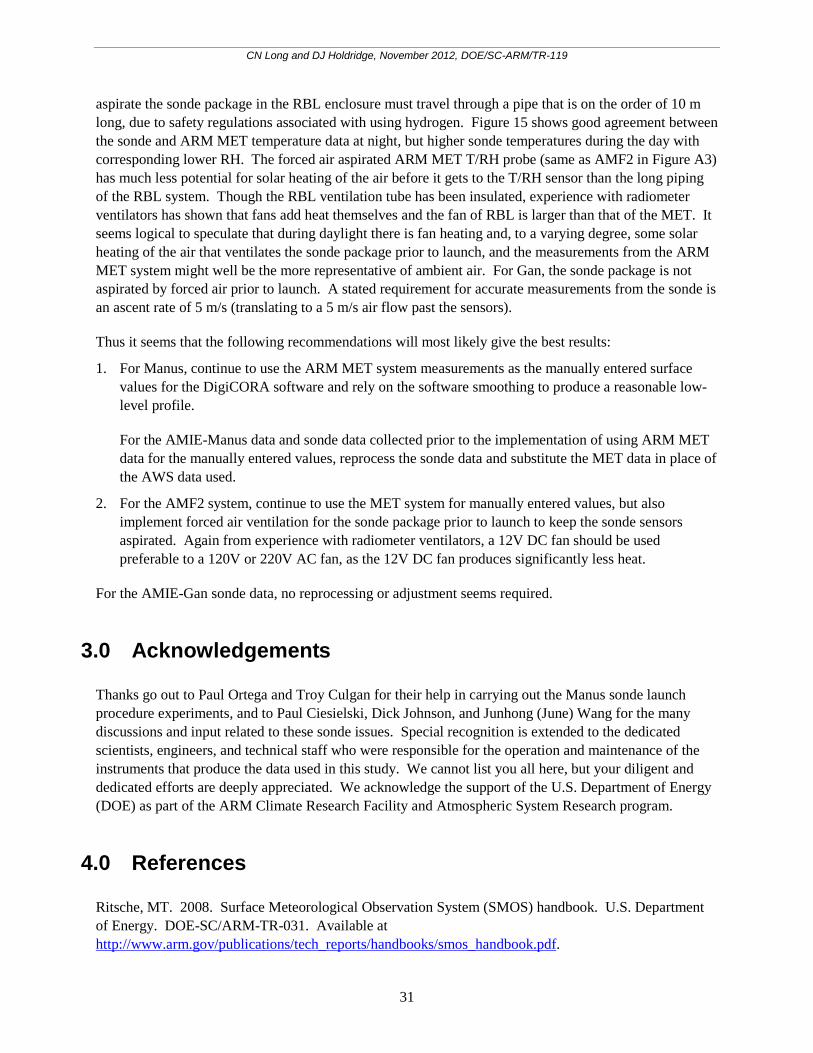
All of the above calculations use data from a very shallow layer near the surface. For Manus, the surface to 1000 mb layer covers 6 mb on average, with the detected temperature inversions covering 7 mb on average. For Gan, the surface to 1000 mb covers 9 mb on average, and the far fewer detected inversions cover 4 mb on average. (See Figure A1 for plots of these pressure depths by time of day for both sites.)

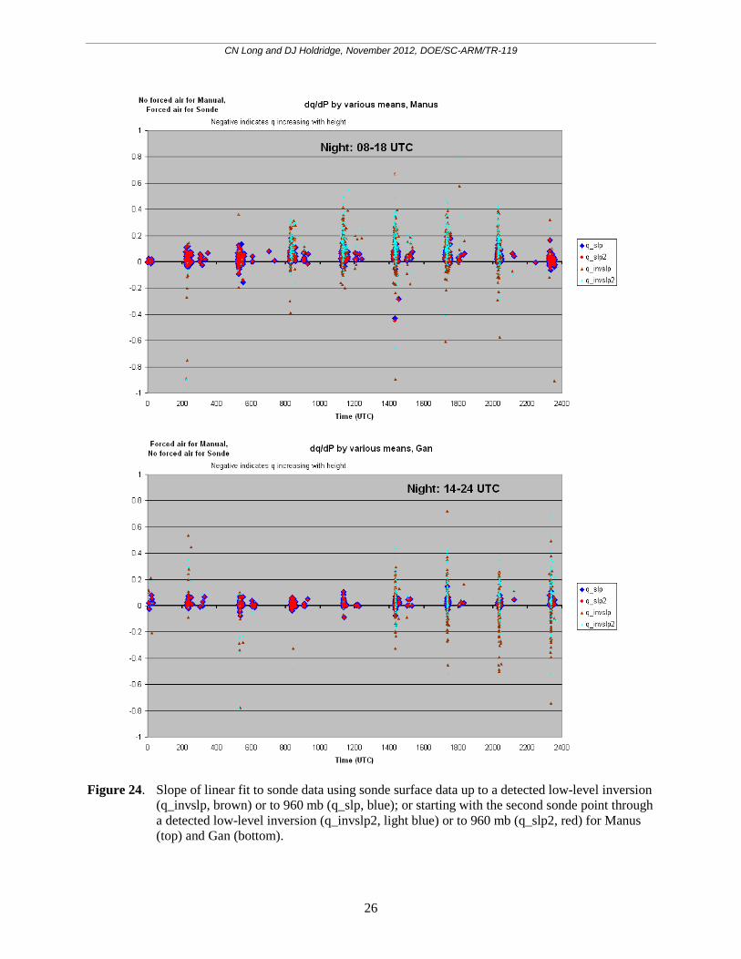
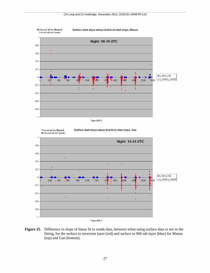
Figure 24 shows results of the slope of a linear fit through the data using sonde surface data up to a detected low-level inversion (q_invslp, brown) or to 960 mb (q_slp, blue), or starting with the second sonde point through a detected low-level inversion (q_invslp2, light blue) or to 960 mb (q_slp2, red). For Manus (top plot) most slopes are positive day and night. The inversion slopes exhibit wider scatter in the results, while the slopes for the surface to 960 mb layer are all of smaller magnitude. Whether the surface value is included in the slope calculation or not makes some difference for the shallow inversion calculations, with not using the surface sonde data eliminating a few of the negative values. But whether the surface value is used or not makes virtually no difference for the surface to 960 mb layer slopes. Figure 25 shows the slope differences produced whether using the surface data in the linear fitting or not (with minus without). For Manus (top) Figure 25 confirms that the slope calculated without the surface data is by far most often more positive, producing a negative “with minus without” difference, while the difference for the surface to 960 mb layer calculations are always very small.


26

Figure 24. Slope of linear fit to sonde data using sonde surface data up to a detected low-level inversion

(q_invslp, brown) or to 960 mb (q_slp, blue); or starting with the second sonde point through a detected low-level inversion (q_invslp2, light blue) or to 960 mb (q_slp2, red) for Manus (top) and Gan (bottom).


27

Figure 25. Difference in slope of linear fit to sonde data, between when using surface data or not in the

fitting, for the surface to inversion layer (red) and surface to 960 mb layer (blue) for Manus (top) and Gan (bottom).


28

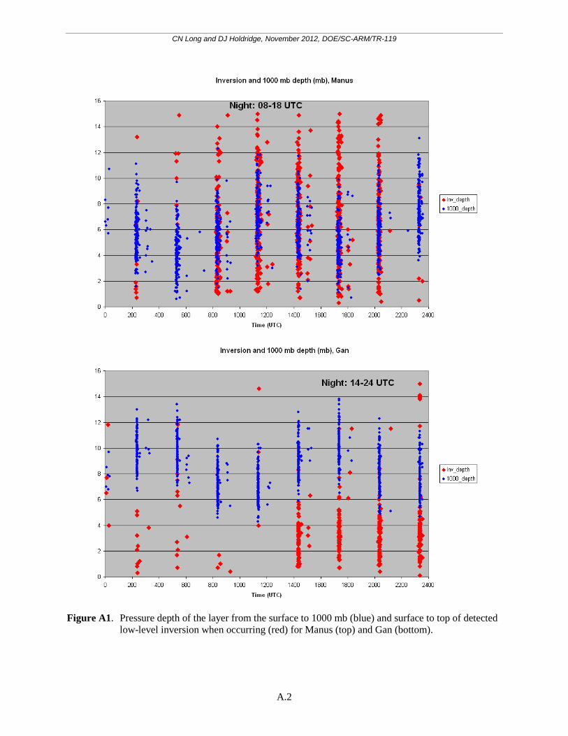
For Gan the shallow inversion slopes exhibit both positive and negative values (Figure 24, bottom), again with some negative values eliminated when the surface value is not included in the calculation. The differences between “with or without” the surface data point also have a greater effect (Figure 25, bottom) than at Manus. This result is most likely due to the shallowness of the Gan inversions that cover only 4 mb on average (Figure A1) and thus for Gan, the difference in q value from the surface to inversion top is significantly smaller than those for the deeper Manus inversions (7 mb on average) and certainly falls within the uncertainty of the q calculations. Therefore, even a small error or bias in the sonde measurements has a larger influence on these slopes. (See Figure A2 for the surface to inversion top q differences by time of day for both sites.) Again, whether the surface value is used or not makes virtually no difference for the surface to 960 mb layer slopes (Figures 24 and 25, bottom).

2.2 Summary and Conclusions

As presented at the February 2012 CINDY/DYNAMO/AMIE Sounding Data Workshop, convincing evidence exists that shallow low-level temperature inversions at Manus are real and occur frequently at night. The inversions are produced whether the final output from the DigiCORA V3.64 software that includes either of the following:

• the surface manually entered measurements and the “smoothing” of the lower level data plus solar heating and dry bias corrections

• the “raw” sonde data from the PTU files used here and either measurements from the Manus ARM surface SMET system (rather than the Manus AWS system measurements used for the manually entered values up through the end of February 2012) or the surface sonde data instead.

The strength of these inversions is related to wind speeds at both Manus and Gan (Figure 20) with Manus winds being generally fairly calm at night.

The shallow inversions at Manus generally exhibit a similar pressure depth as the surface to 1000 mb layer (Figure A1), thus dq/dP slope calculations are also similar (Figure 21 and Figure 24 top). The same is not true for Gan, where the inversions usually are much shallower than the surface to 1000 mb layer, and thus the latter slope calculations (Figure 23) are somewhat better behaved than the inversion layer slope calculations (Figure 24 bottom).

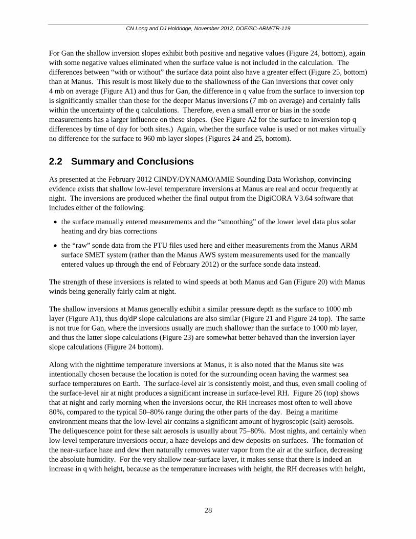
Along with the nighttime temperature inversions at Manus, it is also noted that the Manus site was intentionally chosen because the location is noted for the surrounding ocean having the warmest sea surface temperatures on Earth. The surface-level air is consistently moist, and thus, even small cooling of the surface-level air at night produces a significant increase in surface-level RH. Figure 26 (top) shows that at night and early morning when the inversions occur, the RH increases most often to well above 80%, compared to the typical 50–80% range during the other parts of the day. Being a maritime environment means that the low-level air contains a significant amount of hygroscopic (salt) aerosols. The deliquescence point for these salt aerosols is usually about 75–80%. Most nights, and certainly when low-level temperature inversions occur, a haze develops and dew deposits on surfaces. The formation of the near-surface haze and dew then naturally removes water vapor from the air at the surface, decreasing the absolute humidity. For the very shallow near-surface layer, it makes sense that there is indeed an increase in q with height, because as the temperature increases with height, the RH decreases with height,


29

producing a decrease in haze formation with height and a corresponding decrease in the removal of water vapor with height. It is stressed that this is a very shallow depth near-surface phenomenon.

Figure 26. Surface RH at sonde launch time from the manually entered values (blue) and the sonde

surface measurements (red) for Manus (top) and Gan (bottom). Yellow line represents a 21-point running mean through the sonde data as a visual aid.


30

The situation is not the same for Gan, where the low-level inversions are far less frequent, and the surface RH values are on average significantly lower than those at Manus at night as shown in Figure 26 (bottom). While there are occurrences of surface RH at and above the deliquescence point for salt aerosols, they are far less frequent than at Manus. While nighttime occurrences of increasing q with height do occur in the Gan data, it is not the more prevalent mode as it is at Manus.

As for the calculation of dq/dP (or dq/dz), this study suggests that using the slope of a fitted line is more representative of the actual overall average change in q with height than using a finite difference approach anchored in the surface value as one component of the differences, even when using an average for the above surface-layer value. This is especially true when the data used are over a very small depth of the lower atmosphere, where the vagaries of sonde data at launch (given the initial ascent and uncertainties associated with the required aspiration of the sonde sensors by passing through the atmosphere) and the uncertainties and thus differences between surface meteorological systems measurements and sonde surface readings can have a significant impact on the results for such a shallow layer.

However, it is recognized that in the field there are situations where only GTS data are available, such as for DYNAMO. In those cases care should be exercised in using and interpreting the finite difference results. In the Manus case, the frequent nighttime inversions produced a first “significant” level such that the finite difference calculations there often included an increase in q with height. For Manus this is physically realistic due to surface haze and dew formation at night. But comparing the Manus results to other sites where this does not occur nearly as frequently or at all can lead to confusion in interpretation of the comparison results, because the depth represented in the GTS finite difference calculation is greater and without frequent occurrence of q increasing with height in a shallow layer. In these cases, it might be prudent to pay attention to the typical heights that are involved in the near-surface dq/dz calculations from the GTS messages as an aid to interpretation of the comparisons to help detect when the comparisons encompass a significant “apples to oranges” component. Perhaps using the first mandatory level in the GTS files for all sites rather than the somewhat arbitrary first level whether mandatory or significant might help.

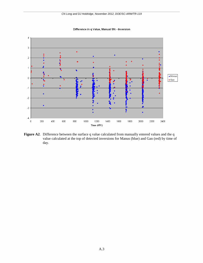
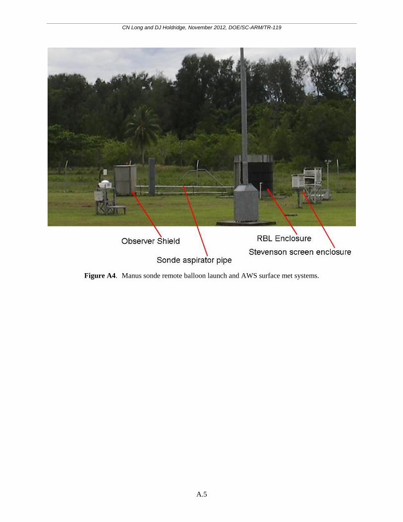
The question has been raised as to whether using the surface manually entered data or the sonde surface data might give “better” results for constructing the lower levels of the sonde profiles for Manus, and also for Gan. The AMF2 system uses a forced air aspirated enclosure for the MET system T and RH probe, while the sonde package sits on a shelf in the open air prior to launch while the balloon is being filled (see Figure A3). Manus uses a RBL system (due to using hydrogen gas) that includes forced air aspiration of the sonde package prior to launch while the balloon is filled, and for most of the AMIE campaign, Manus used surface met data from an Australian AWS system in a standard Stevenson screen enclosure that did not have forced air ventilation (see Figure A4). As presented at the February 2012 CINDY/DYNAMO/AMIE Sounding Data Workshop, the agreement between the Manus AWS met system data and sonde surface data compared to the agreement between the sonde surface data and that from the ARM forced air ventilated MET system similar to that of the AMF2 showed better agreement when using the forced air MET system. This result then drove the switch from using the AWS data for the surface data manually entered into the DigiCORA sonde system to instead using data from the ARM MET system. The improvement in manually entered and sonde surface agreement is suggested in Figure 15.

However, Figure 15 also shows that there is still some disagreement larger than that exhibited for the Gan data (Figure 14, bottom) especially for temperature. As can be seen in Figure A4, the air that is forced to


31

aspirate the sonde package in the RBL enclosure must travel through a pipe that is on the order of 10 m long, due to safety regulations associated with using hydrogen. Figure 15 shows good agreement between the sonde and ARM MET temperature data at night, but higher sonde temperatures during the day with corresponding lower RH. The forced air aspirated ARM MET T/RH probe (same as AMF2 in Figure A3) has much less potential for solar heating of the air before it gets to the T/RH sensor than the long piping of the RBL system. Though the RBL ventilation tube has been insulated, experience with radiometer ventilators has shown that fans add heat themselves and the fan of RBL is larger than that of the MET. It seems logical to speculate that during daylight there is fan heating and, to a varying degree, some solar heating of the air that ventilates the sonde package prior to launch, and the measurements from the ARM MET system might well be the more representative of ambient air. For Gan, the sonde package is not aspirated by forced air prior to launch. A stated requirement for accurate measurements from the sonde is an ascent rate of 5 m/s (translating to a 5 m/s air flow past the sensors).

Thus it seems that the following recommendations will most likely give the best results:

1. For Manus, continue to use the ARM MET system measurements as the manually entered surface values for the DigiCORA software and rely on the software smoothing to produce a reasonable low-level profile.

For the AMIE-Manus data and sonde data collected prior to the implementation of using ARM MET data for the manually entered values, reprocess the sonde data and substitute the MET data in place of the AWS data used.

2. For the AMF2 system, continue to use the MET system for manually entered values, but also implement forced air ventilation for the sonde package prior to launch to keep the sonde sensors aspirated. Again from experience with radiometer ventilators, a 12V DC fan should be used preferable to a 120V or 220V AC fan, as the 12V DC fan produces significantly less heat.

For the AMIE-Gan sonde data, no reprocessing or adjustment seems required.

3.0 Acknowledgements

Thanks go out to Paul Ortega and Troy Culgan for their help in carrying out the Manus sonde launch procedure experiments, and to Paul Ciesielski, Dick Johnson, and Junhong (June) Wang for the many discussions and input related to these sonde issues. Special recognition is extended to the dedicated scientists, engineers, and technical staff who were responsible for the operation and maintenance of the instruments that produce the data used in this study. We cannot list you all here, but your diligent and dedicated efforts are deeply appreciated. We acknowledge the support of the U.S. Department of Energy (DOE) as part of the ARM Climate Research Facility and Atmospheric System Research program.

4.0 References

Ritsche, MT. 2008. Surface Meteorological Observation System (SMOS) handbook. U.S. Department of Energy. DOE-SC/ARM-TR-031. Available at http://www.arm.gov/publications/tech_reports/handbooks/smos_handbook.pdf.

http://www.arm.gov/publications/tech_reports/handbooks/smos_handbook.pdf


A.1

Appendix A


A.1

Appendix A

Table A1. Listing and description of the various dq/dP calculations used in this study.


A.2

Figure A1. Pressure depth of the layer from the surface to 1000 mb (blue) and surface to top of detected

low-level inversion when occurring (red) for Manus (top) and Gan (bottom).


A.3

Figure A2. Difference between the surface q value calculated from manually entered values and the q

value calculated at the top of detected inversions for Manus (blue) and Gan (red) by time of day.


A.4

Figure A3. AMF2 sonde launch and surface MET systems.


A.5

Figure A4. Manus sonde remote balloon launch and AWS surface met systems.

Documents

Investigations of Possible Low-Level Temperature and