Embed Size (px)
Citation preview

Investigations of counter propagating laser
produced plasmas in a collision free system in the
presence of a strong external magnetic field.
Volume 1 of 1
Robert Alan David Grundy
Doctor of Philosophy
The University of York
Department of Physics
September 2003
2
2
Abstract
This thesis presents a beginning of an investigation into the formation of a collisionless
shock through the interaction of two rapidly expanding laser-produced plasmas
immersed in a strong magnetic field. The ultimate aim is to produce an experimental
simulation that can be scaled to be relevant to a 100-year-old Supernova remnant. This
requires the reproducible production of plasmas with low densities (~1018cm-3) and high
expansion velocities (~107cm/s) in a counter propagating geometry.
The chosen method of forming this simulation is the production of plasma by the direct
drive laser irradiation at 1014W/cm2 of 100nm thick solid targets. The experiments are
diagnosed primarily by optical probing techniques, the principal theme of this thesis.
These results show evolution of the plasma is in good agreement with both analytical
and numerical models.
However, the plasma produced by direct drive irradiation was found to be structured.
The observed structure is primarily a result of laser imprint, and experimental
techniques have been developed to overcome this using a spatially filtered pre-pulse.
With the ability to produce uniform, well characterised plasma we are able to
demonstrate that immersing thin foil plasma in a strong (~10T) magnetic field does not
affect the hydrodynamics of the plasma. When produced in a counter-propagating
geometry, two thin foil plasmas can be shown to interpenetrate in a collisionless
manner. Immersing this system in a strong magnetic field alters the interaction. Instead
of interpenetrating, the plasmas behave similarly to a collision-dominated counter-
propagating system.
The mechanism by which this occurs is still uncertain. However, if this change in
system behaviour is caused by the magnetic field penetrating into that plasma and
localising the particles on a scale smaller than that of binary collisions, then it may be
feasible to produce a scaled experimental simulation of a Supernova remnant using this
technique.

3
3
List of contents
ABSTRACT.................................................................................................................................. 2
LIST OF CONTENTS .................................................................................................................. 3
LIST OF ILLUSTRATIONS........................................................................................................ 8
ACKNOWLEDGEMENTS........................................................................................................ 13
AUTHOR’S DECLARATION................................................................................................... 15
CHAPTER 1 - INTRODUCTION.............................................................................................. 16
1.1 MOTIVATION.................................................................................................................. 16
1.2 BACKGROUND................................................................................................................ 17
1.2.1 Laboratory Astrophysics ....................................................................................... 17
1.2.2 Thin foil laser produced plasmas .......................................................................... 19
1.2.3 Colliding plasma experiments............................................................................... 20
1.3 CHAPTER OUTLINE......................................................................................................... 22
CHAPTER 2 - THEORY............................................................................................................ 24
2.1 INTRODUCTION .............................................................................................................. 24
2.2 PLASMA PARAMETERS ................................................................................................... 25
2.2.1 Collective effects ................................................................................................... 25
2.2.2 Single Particle Motions......................................................................................... 27
2.2.3 Plasma Oscillations .............................................................................................. 31
2.3 COLLISIONALITY............................................................................................................ 32
2.4 COLLISIONLESS SHOCKS ................................................................................................ 35
2.4.1 Shock formation .................................................................................................... 35

4
4
2.4.2 Shock conditions.................................................................................................... 36
2.4.3 Shock thickness...................................................................................................... 38
2.5 SCALING......................................................................................................................... 40
2.6 LASER-PLASMA INTERACTIONS...................................................................................... 44
2.7 CONCLUSIONS ................................................................................................................ 50
CHAPTER 3 - OPTICAL PROBES. .......................................................................................... 52
3.1 INTRODUCTION .............................................................................................................. 52
3.2 THEORY OF PROPAGATION OF LIGHT IN AN UNDER-DENSE PLASMA.............................. 53
3.2.1 The refractive index of a plasma ........................................................................... 54
3.2.2 Propagation of light in geometrical optics approximation ................................... 57
3.3 THE VULCAN LASER SYSTEM ........................................................................................ 58
3.4 PROBE BEAMS ................................................................................................................ 59
3.4.1 Utilised probe beam designs ................................................................................. 59
3.4.2 Temporal resolution requirements ........................................................................ 62
3.4.3 Wavelength selection............................................................................................. 64
3.4.4 Intensity selection.................................................................................................. 65
3.4.5 Wavefront quality .................................................................................................. 66
3.5 IMAGING SYSTEMS......................................................................................................... 67
3.5.1 Resolution requirements........................................................................................ 69
3.5.2 Diffraction around target, diffraction limit........................................................... 71
3.5.3 Imaging for Interferometry.................................................................................... 73
3.5.4 Limitations due to refraction................................................................................. 75
3.6 CONCLUSIONS ................................................................................................................ 75

5
5
CHAPTER 4 - OPTICAL PROBE DIAGNOSTICS.................................................................. 76
4.1 INTRODUCTION .............................................................................................................. 76
4.2 INTERFEROMETRY.......................................................................................................... 76
4.2.1 Theory ................................................................................................................... 76
4.2.2 Interferometer Designs.......................................................................................... 79
4.2.3 Interferometery Analysis Technique...................................................................... 81
4.2.4 Abel inversion........................................................................................................ 85
4.3 SHADOWGRAPHY AND SCHLIEREN IMAGING................................................................. 87
4.3.1 Theory ................................................................................................................... 87
4.3.2 Schlieren Designs.................................................................................................. 88
4.3.3 Ray tracing analysis .............................................................................................. 89
4.3.4 Code design........................................................................................................... 90
4.3.5 Benchmarking the code. ........................................................................................ 91
4.3.6 Producing simulated schlieren images. ................................................................ 97
4.3.7 Analysis of the ray tracing .................................................................................... 98
4.4 POLARIMETRY.............................................................................................................. 100
4.4.1 Theory ................................................................................................................. 100
4.4.2 Polarimeter Designs............................................................................................ 104
4.4.3 Polarisation analysis code .................................................................................. 105
4.5 CONCLUSIONS .............................................................................................................. 108
CHAPTER 5 - PRODUCING PLASMA FROM A SINGLE THIN FOIL.............................. 110
5.1 INTRODUCTION ............................................................................................................ 110

6
6
5.2 EXPERIMENTAL TECHNIQUE ........................................................................................ 111
5.2.1 Introduction......................................................................................................... 111
5.2.2 Target Design and Manufacture ......................................................................... 111
5.2.3 Experimental Setup ............................................................................................. 112
5.3 RESULTS....................................................................................................................... 115
5.3.1 Expansion............................................................................................................ 115
5.3.2 Density Profile .................................................................................................... 117
5.3.3 Plasma non-uniformity........................................................................................ 120
5.3.4 Laser focussing conditions .................................................................................. 123
5.3.5 Target characterisation....................................................................................... 125
5.4 DISCUSSION.................................................................................................................. 128
5.4.1 Comparison of Expansion with models ............................................................... 128
5.4.2 Plasma non-uniformity........................................................................................ 130
5.4.2.1 Target structure ............................................................................................... 130
5.4.2.2 Laser focal spot intensity structure ................................................................. 132
5.4.3 Thermal smoothing.............................................................................................. 133
5.5 PLASMA SMOOTHING EXPERIMENT.............................................................................. 135
5.5.1 Experimental set up............................................................................................. 136
5.5.2 Results ................................................................................................................. 137
5.5.3 Discussion ........................................................................................................... 139
5.6 CONCLUSIONS .............................................................................................................. 139
CHAPTER 6 - COLLIDING MAGNETISED FOILS ............................................................. 140
6.1 INTRODUCTION ............................................................................................................ 140

7
7
6.2 PRODUCTION OF A MAGNETIC FIELD............................................................................ 140
6.2.1 Helmholtz coil laser target.................................................................................. 141
6.2.2 Pulsed power electromagnet ............................................................................... 146
6.3 SINGLE FOIL EXPANSION IN A MAGNETIC FIELD........................................................... 148
6.4 COUNTER PROPAGATING EXPLODING FOIL PLASMAS .................................................. 151
6.4.1 Counter propagating CH foils............................................................................. 152
6.4.2 Counter propagating Al foils............................................................................... 154
6.5 MAGNETISED COUNTER PROPAGATING PLASMAS........................................................ 156
6.6 DISCUSSION.................................................................................................................. 159
6.7 CONCLUSIONS .............................................................................................................. 164
CHAPTER 7 - CONCLUSIONS .............................................................................................. 166
7.1 CONCLUSIONS .............................................................................................................. 166
7.2 FURTHER WORK........................................................................................................... 168
REFERENCES ......................................................................................................................... 170
8
8
List of illustrations
Figure 2.1 Diagram of the temperature and density scales of different plasmas 44
Figure 2.2 Med103 simulations of the proposed colliding foils scheme 49
Figure 2.3 Scaling parameters for a 100 year old SNR. 50
Figure 3.1 Processes that occur during propagation of a laser through a plasma 53
Figure 3.2 Probe front-end layouts for each experiment 60
Figure 3.3 Schematic of a grating pair arranged for pulse compression 62
Figure 3.4 The effect of a mismatched gratings 63
Figure 3.5 Probe beam pulse shapes 64
Figure 3.6 Near field intensity pattern of the probe from the second experiment 66
Figure 3.7 First experimental imaging system layout 67
Figure 3.8 Second experimental imaging system 68
Figure 3.9 Third experimental imaging system. 69
Figure 3.10 Modulation Transfer functions for the three imaging 70
Figure 3.11 The comparison between theoretical and observed 72
Figure 3.12 OPD plots for the three imaging systems 74
Figure 4.1 Simulated interference pattern 78
Figure 4.2 Principle of a Wollaston prism based interferometer. 80
9
9
Figure 4.3 Schematic of an imaging Wollaston prism based interferometer 80
Figure 4.4 Principle of the vertical shearing interferometer 81
Figure 4.5 Rotating an interferogram to allow fringe extraction 82
Figure 4.6 The process of fringe extraction to produce a phase difference plot 83
Figure 4.7 Sample interferogram and extraction of the electron density 84
Figure 4.8 Broadband emission from a 200µm diameter Al dot 86
Figure 4.9 Contour plots of electron density data 86
Figure 4.10 Schlieren imaging schematic 88
Figure 4.11 Schlieren imaging arrangement for second experiment 89
Figure 4.12 Geometry of the ray tracing code 90
Figure 4.13 Spherical plasma geometry and radial electron density 92
Figure 4.14 Values of the calculated minimum radius compared with simulation 93
Figure 4.15 Variation of the impact parameter B with respect to the initial 94
Figure 4.16 Results of the modified ray tracing 96
Figure 4.17 Variation of the impact parameter for comparison Figure 4.15 97
Figure 4.18 Back propagation of rays onto a CCD at the assumed object plane 98
Figure 4.19 Forming a simulated schlieren image 99
Figure 4.20 Ray traced image overlaid on experimental schlieren data 99
Figure 4.21 Wollaston prism based polarisation analyser. 105
Figure 4.22 Statistical error in the calculation 107
Figure 4.23 Polarimeter testing for various input polarisation angles. 107
10
10
Figure 5.1 Design of the target holder used in all experiments 112
Figure 5.2 Generic plan of the target chamber layout for single foil experiments. 113
Figure 5.3 Focal spot imaging 115
Figure 5.4 Graph of plasma expansion, 116
Figure 5.5 Interferometric images of 100nm thick CH foils 118
Figure 5.6 Abel inverted electron density profiles 119
Figure 5.7 Schlieren images from the first experiment 121
Figure 5.8 Schlieren images taken during the second experiment. 121
Figure 5.9 Detail of high resolution schlieren 122
Figure 5.10 X-ray pinhole camera images 122
Figure 5.11 Normalised focal spot 123
Figure 5.12 2D FFT Power spectra 124
Figure 5.13 Electron micrographs of a CH foil and a Al foil on a Mylar holder 125
Figure 5.14 Electron micrographs of a CH foil and a Al foil on a Cu holder 126
Figure 5.15 High magnification electron micrograph of a CH foil a Cu holder 126
Figure 5.16 Laser interferogram of a CH foil mounted on a Cu holder 127
Figure 5.17 Graph of the analytical model interferometry measurements 128
Figure 5.18 Graph of Medusa simulation compared with experimental data 129
Figure 5.19 Schlieren Image lineouts across the schlieren images in Figure 5.9 131
Figure 5.20 Vertical lineouts across the schlieren images in Figure 5.7 132
11
11
Figure 5.21 Vertical Lineouts across the schlieren images in Figure 5.8 133
Figure 5.22 Experimental chamber layout for pre-pulse experiments 136
Figure 5.23 Evidence of pre-pulse smoothing 138
Figure 6.1 Production of a magnetic field through use of a laser target. 142
Figure 6.2 Photograph of the Helmholtz coil target geometry 143
Figure 6.3 Single turn search coil results from our first experiment 144
Figure 6.4 Interferogram of two foils and a Helmholtz coil taken 145
Figure 6.5 Schlieren data taken 500ps after foil irradiation. 145
Figure 6.6 The construction of the pulsed electromagnet 146
Figure 6.7 Polarogram of a glass slide inside the pulsed electromagnet 147
Figure 6.8 Evolution of the magnetic field in the electromagnet 148
Figure 6.9 Experimental chamber plan for magnetised single foil experiments. 149
Figure 6.10 Interferograms taken 750ps after target 150
Figure 6.11 Abel inverted thin CH foil electron density profiles 150
Figure 6.12 Experimental layout for counter-propagating thin foil experiments 152
Figure 6.13 Interferogram of the interaction of two counter propagating 153
Figure 6.14 Expansion of two CH foils compared to two single foils 153
Figure 6.15 Schlieren data with the ray-traced simulation overlaid 154
Figure 6.16 Interferogram of two Al foils taken 750ps after irradiation. 155
Figure 6.17 Expansion of two Al foils compared to two single foils 155

12
12
Figure 6.18 Arrangement for counter propagating experiments in a magnetic field 156
Figure 6.19 Interferogram of two CH foils immersed in a 7.5T magnetic field 157
Figure 6.20 Comparison of magnetised and non-magnetised colliding foil data 158
Figure 6.21 Interferometry reference channel image 158
Figure 6.22 Shadowgraph from a Helmholtz experiment 159
Figure 6.23 Comparison of Medusa simulation with the experimental profile 161
Figure 6.24 The expansion of two magnetised CH foils and two Al foils. 162
Figure 6.25 Abel inverted radial density gradient profile 164

13
13
Acknowledgements
Firstly, I would like to express my sincere thanks to Dr Nigel Woolsey for his guidance
and supervision of this thesis. I would also like to thank Professor Greg Tallents for his
supervision during the first years of my work. I am deeply grateful to Dr Cedric
Courtois, Dr Dave Chambers and Andrew Ash with whom it has been my great pleasure
to work with.
Special thanks also go to Yousef Abou-Ali and Dr Jalal Pechtehe for their contribution
to our experiments and companionship in our office and to Dr Stephen Tear for his
assistance and use of the Scanning Electron Microscope.
The experimental work would not have been possible without the help and goodwill of
the staff of the VULCAN laser at the Rutherford Appleton Laboratory, my thanks to
you all. In particular I would like to thank Margaret Notley, Rob Heathcote and Rob
Clarke for their assistance and advice when performing experiments. I would also thank
Dr John Collier for his assistance with designing optics and use of the Zeemax design
package.
I would also express my thanks to Dr Richard Dendy, Dr Per Hellander and Dr Ken
McClemments of the Culham Science Centre for their collaborative work with our
group and useful discussions. In addition, I would also express my thanks the Dr Paddy
Carrolan and Dr Neil Conway for their experimental collaboration and advice on
Zeeman splitting diagnostics.
For their collaboration in our final experiment, I would also like to thank Ben Lings and
Katarina Rosol’ankova of the University of Oxford.
Finally, I am grateful for the support and encouragement provided by my family and
friends, especially my partner Amber. Without you, this would not have been possible.

14
14
In memory of my father.

15
15
Author’s declaration
The work presented in this thesis is the product of the work of many people, the nature
of the laser-plasma experiments presented is such that they require a collaborative
research group using large-scale facilities. This not only includes the members of the
experimental teams, but also the facility staff and our collaborators.
Here I will outline the contribution I have made within the group. My primary role has
been that of an experimentalist, contributing to the planning and execution of our
experimental work. In the main part, this has been through the development and
utilisation of optical probing techniques and the associated diagnostics. I have carried
out all of the analysis of the data collected by these diagnostics and assisted in its
interpretation in conjunction with other diagnostics used. To this end, I have also been
responsible for the development of an iterative ray tracing code to simulate the optical
probe, and codes to simulate and analyse the diagnostic data. I have also carried out
investigations of the thermal smoothing techniques in thin foil plasma and of the
performance of our optical probe imaging.
The plasma simulation work quoted throughout the thesis (unless otherwise stated) is
the work of my supervisor, Dr Woolsey. The focal spot profile measurements in
Chapter 5 and the magnetic field calculations and Faraday cups measurements quoted in
Chapter 6 are the work of Dr Woolsey and Dr Courtois.

16
16
1 Chapter 1 - Introduction
1.1 Motivation
Astrophysical research has been traditionally based in theoretical modelling and
observational data. Traditionally the contribution of experimental physics to this
research has been in the main part through measuring the fundamental parameters of
atomic and molecular physics.
Developments in high-energy density physics experiments1 now enable us to produce
conditions in the laboratory that are relevant to astrophysical systems. This permits us to
perform laboratory astrophysics experiments to provide an accurate basis for theoretical
modelling such as equation of state2 and radiation transfer measurements3. These
provide the ‘inputs’ for astrophysical modelling. This also introduces the possibility of
producing a scaled4 reproduction of an astrophysical system in the laboratory,5 which
can be used to test the predictions of theories or the ‘outputs’ of astrophysical
modelling, and be compared with observational data.
Many different types of plasma production technique have been used, from wire-array
z-pinches6 to high power lasers1,7, covering a range of astrophysical systems from jet
formation6,8,9 to supernova remnants10.
One of the current unanswered questions in astrophysics is the source and acceleration
of cosmic rays. The observed spectra of cosmic rays may be produced by the
combination of two separate sources11. It is proposed that the production of cosmic rays
above an energy of 1019eV may be the result of acceleration by intergalactic magnetic
recombination events12. This type of system has been studied experimentally13 using
two spheromaks. These experiments have shown particles being significantly
accelerated by magnetic recombination.
Cosmic rays of energy lower than 1015 eV are widely assumed to by produced by
diffusive shock acceleration (DSA)14 across the shock front15 of a supernova16.
Characteristic X-ray synchrotron radiation of 1014eV fitting the theoretical spectra for
DSA has been observed17 in the vicinity of the supernova remnant SN1006. However,
the mechanism by which particles are ‘injected’ into the process of DSA is
17
17
unknown18,19. It has been proposed that the collisionless shock20 system of such a
supernova remnant required to simulate this phenomenon is within the reaches of
experimental possibility21.
The aim of this research reported here is to develop the capability to perform an
experimental simulation of a 100 year old supernova remnant, by use of a high power
laser. The laser is used to irradiate two thin foil plasmas in an opposing geometry
immersed in a strong magnetic field.
1.2 Background
The scope of this thesis primarily covers the production of plasma from thin foils in a
counter-propagating geometry and in the presence of a magnetic field. The setting for
this work is the field of laboratory astrophysics, which has already been touched upon in
the previous section. In this section, I will place the work presented in this thesis in the
context of the previous work that has been performed in these related fields. To this end,
this section is divided into three sections: laboratory astrophysical research relevant to
the production of a simulation of a 100 year old supernova remnant, laser-plasma
research into production of thin foil laser-plasmas, and research into the interactions of
plasmas in a colliding geometry.
1.2.1 Laboratory Astrophysics
The field of laboratory astrophysics using intense lasers has been reviewed by Rose7,
Ripin et al22, Remington et al23 and Takabe et al24. The specific field of collisionless
laboratory astrophysics has also been reviewed by Zakharov25.
The ultimate aim of the research project is to perform an experimental simulation of a
100 year old supernova remnant (SNR). This differs from previous scaled supernova
experiments reviewed by Drake26, since we are attempting only to produce simulation
snapshot of the SNR as opposed to modelling the evolution of the system (see Chapter
2, section 2.5). Previous experiments by Drake et al27,28 have modelled a young
supernova remnant, SN1987A, where the explosion of the supernova will collide with a
circumstellar ring. The supernova is simulated by the explosion by indirect drive (using
a gold hohlraum) of a plastic ‘plug’. The plasma formed by this method is allowed to
expand through a vacuum until it collides with a foam target, which models the
18
18
circumstellar ring. Experiments by Kane et al29 have also studied hydrodynamic
instabilities that play a critical role in the evolution of a core collapse supernovae, such
as SN1987A. In this stage of supernova remnant evolution the shock produced is
radiative, a system which has been studied by Shigemori et al30.
After the initial explosion of the supernova, the shock wave expands into the interstellar
medium (ISM)31. The interaction of the SNR shock with interstellar clouds has been
investigated by Klein et al32. The expansion of the SNR into the ISM is actually
comprised of two shocks16, the forward shock of the explosion and a reverse shock
travelling backwards through the ejecta. Although the reverse shock is propagating
towards the centre of the SNR, the expansion of the ejecta is much faster than the
reverse shock, which is therefore carried outwards. When the amount of material swept
up by the SNR shock is roughly of mass equivalent to that of the ejecta, then the reverse
shock is no longer carried outwards by the expansion, and propagates inwards. It is this
stage in the SNR evolution that we are interested in studying. The key feature of this
stage of SNR evolution is the formation of a magnetised, non-radiative collisionless
shock.
A collisionless shock is a shock where the thickness of the shock transition from the
upstream to downstream state (see Chapter 2) is less than the ion-ion binary collision
mean free path. As will be described in Chapter 2, collisionless shocks require a
dissipative mechanism, with a corresponding scale length, for this transition to occur.
Early collisionless shock experiments33 supported by simulations34 focussed on the
formation of an electrostatic collisionless shock, where the scale length of the shock is
the Debye length, λD. A shock thickness of 5λD was observed33 in a plasma where the
binary collision mean free path was 103λD. Laser-plasma experiments to produce
electrostatic collisionless shocks were performed by Koopman and Tidman35. A 15ns 3J
pulse from a ruby laser was used to irradiate a solid cluster target driving a spherical
expansion into an ambient background plasma. A shock thickness of 0.1cm was
observed compared to the mean free path of 10cm.
This type of collisionless interaction between counter-propagating ions was also studied
by Dean et al36 again using a laser-plasma produced from a solid target expanding into a
photo-ionised background gas. These results were found to agree with the prediction of
the interaction as a ion-ion two-stream instability37 in the presence of a self generated

19
19
magnetic field. However, there was debate over the validity of the collisionless nature
of the system38,39.
In a similar experiment by Cheung et al,40 collisionless coupling in inter-penetrating
plasmas was observed in the presence of a magnetic field. Experimental evidence shows
that the magnetic field introduces turbulent effects and produces features resembling
collisional results, which do not exist without the magnetic field.
Laser-plasma experiments by Bell et al41 formed a magnetised collisionless shock by
colliding a magnetised laser produced plasma with a solid obstacle. The plasma is
generated by laser ablation of a solid Carbon target producing a spherically expanding
plasma. The plasma at a density of ~1018cm-3 impinges on a spherical carbon obstacle in
a 10kG magnetic field. The ratio of thermal to magnetic pressure, the plasma β, is
around 300 in this case, and the mean free path is 1mm. A bow shock was observed
with a thickness of between 10 and 50µm, comparable to the 70µm electron Larmor
radius (see Chapter 2, section 2.2.2), and the 5µm electron skin depth (see Chapter 2,
section 2.4.3). However, this experiment was performed without attempting to scale the
experiment to match an astrophysical system.
The formation of a collisionless shock has been a recurring goal in laser-plasma
physics, and the concept of producing of a system suitable for scaling has inspired new
experimental proposals21 and the work presented in this thesis. The aim of the work
presented here is therefore at the forefront of research within this field.
1.2.2 Thin foil laser produced plasmas
The methodology used in attempting to achieve an experimental simulation of a 100
year old supernova remnant is the formation of plasma from thin foils using a high
power laser. This technique can be employed, as shown by Decoste et al42 to produce
plasmas with high expansion velocities (>107 cm/s). Analytical models of the
hydrodynamics of exploding thin foils are presented by London and Rosen43 and by
Helander et al44. These models are examined in Chapter 2, and are essentially
hydrodynamic treatments of the exploding thin foil expansion.
Historically, thin foils have been used experimentally for many purposes, from X-ray
laser production, e.g. Rosen45, to testing the initial behaviour of inertial confinement

20
20
fusion targets46 and for studies of instabilities in shock waves47. The plasma produced
by direct drive irradiation of thin foils is known to be susceptible to hydrodynamic
instability48,49,50 caused by seed perturbations in either the laser focus51 or in the target
surface. It has been shown by Obenschain et al,52 that the amount of non-uniformity
imprinted into the thin foil from a laser focus is a function of intensity, and by Gardner
and Bodner53, Cole et al54 and Glendinning et al55 that it also scales as a function of
laser wavelength. This susceptibility of thin foils to imprinting makes them ideal tests
for laser smoothing techniques such as induced spatial incoherence56 and smoothing by
spectral dispersion57.
The foils used in our experiments differ from those already discussed in this section by
virtue of their thickness. In the experiments noted previously, the thickness of the foil
material is typically a few microns, whereas the experiments reported in this thesis use
0.1µm thick foils.
1.2.3 Colliding plasma experiments
The interactions between two colliding laser produced plasmas have been studied in the
1970’s by Rumsby et al,58 where two plasmas were formed in adjacent positions on a
Carbon plate, separated by a fixed distance, d. The evolution of two plasmas separated
by d=10mm produces parameters consistent with a Mach 3 hydrodynamic shock
occurring at the interface where the plasmas collide. This results in an observed five-
fold increase in electron density when compared with the evolution of a single plasma.
In this case, the mean free path of the ions in the plasma is estimated to be 6mm, i.e.
shorter than the scale of the experiment. In a second experiment where the separation
distance d=40mm the mean free path of the ions is 400mm, greater than the scale
length, and a density increase of a factor of two is observed. This would correspond to
the addition of the densities of two interpenetrating plasmas.
Theoretical modelling by Berger et al59 using a two ion fluid model of colliding plasmas
shows that for the case of plasmas that are expected to produce a shock, there will be
some degree of interpenetration of the plasmas. This is expected to occur if the scale
length of the velocity gradient in the plasma is shorter than the mean free path. This
interpenetration will subsequently lead to stagnation.
21
21
Experiments to investigate this proposed degree of interpenetration in the collisions of
two laser ablated plasmas were performed by Bosch et al.60 The plasmas were formed
by the ablation of the inner surfaces of two face parallel disks at 1014 W/cm2.
Measurements of the degree of interpenetration were made possible through spatially
resolved spectroscopic measurements of emission from Aluminium (Al) and
Magnesium (Mg) targets in an opposing geometry. The results were found to be in
agreement with the model of Berger et al59, as opposed to a single fluid model.
This model was extended by Rambo and Denavit61 to a multi-fluid model, showing that
the degree of interpenetration can be interpreted in terms of the collisionality parameter
of the system. This collisionality parameter can be described as the ratio of mean free
path of the ions to the scale length of the system, and is discussed further in Chapter 2,
section 2.3. Two experimental schemes are explored: the expansion of plasma ablated
from the front surface of solid disks as used by Bosch et al60, and the interaction of
counter-propagating plasmas produced from the rear surfaces of a pair of thin foils.
These simulations imply that shock formation in a multi-fluid treatment will occur after
a period of soft stagnation, and the shock strengths will be reduced in comparison to the
predictions of a single-fluid model. Numerical simulations by Larroche62 have also
included a kinetic treatment of the period of stagnation. Comparisons between multi-
fluid and kinetic approaches to simulation by Rambo and Procassini63 show that both
treatments produce similar results. Simulations of counter propagating plastic (CH)
plasmas where the carbon and hydrogen components are treated as separate fluids61
show that in a colliding geometry there may be significant separation between the two
species.
Counter-propagating thin foil experiments using volumetric heating of the foils by X-
rays have been performed by Perry et al64. The evolution of counter-propagating Al and
Mg foils in parallel and angled configurations was studied using spectroscopic and x-
ray radiography techniques. The results for the parallel geometry when compared to
radiation hydrodynamic simulations show the peak densities reached during the
collision are lower than predicted, as suggested by Rambo and Denavit61.
The effects of varying the collisionality parameter of a counter propagating exploding
thin foil system was studied by Rancu et al65 and Chenais-Popovics et al66. In this work
~1µm thick Al and Mg foils were separated by 400, 600 or 900µm and irradiated at

22
22
either 3 or 6 x10¹³ W/cm2 at 527nm. This produced a variation in collisionality, as the
dominant term in describing the collisionality in this system is the relative flow velocity
of the colliding plasmas66. Variations from the quasi-collisionless to strongly collisional
regimes with the associated degree of interpenetration are observed.
The experiments reported in this thesis using counter propagating thin foil plasmas also
study the effect of changing the collisionality of the system through the use of different
foil materials. The innovative approach is to also attempt to alter the collisionality
through the effect of an external magnetic field on a CH plasma.
1.3 Chapter Outline
Chapter two describes the fundamental theoretical aspects of plasma physics relevant
to producing plasma by irradiating thin foils using a high power laser. The concepts of
the plasma state will be introduced. This will be discussed in the context of how the
parameters of laboratory produced plasmas can be relevant to an astrophysical plasma
through similarity and scaling arguments. This will be achieved by firstly deriving the
basic parameters that describe a plasma in terms of typical scale lengths and times and
the physics of a collisionless shock. Secondly, the fundamentals of the laser plasma
interaction will be introduced along with analytical models for thin foil plasma
evolution and the numerical simulations undertaken.
Chapter three will develop the theory of the propagation of light through plasma and
the approach of geometric optics. How this affects the design of an optical probe system
for studying low density plasma will be investigated, along with the design criteria for
an optical probe system. Examples of how the optical probe systems are utilised in our
experimental work are discussed. The development of the optical probe for specific
experimental requirements is also outlined.
Chapter four describes the diagnostics used to gain information from an optical probe
in terms of the theory behind the diagnostic, the experimental arrangements used and
the methods utilised to interpret the data. This includes the principal diagnostics of
interferometry, schlieren imaging, shadowgraphy and polarimetry and an iterative ray
tracing code to simulate the passage of light through a plasma. The ray tracing code is
used as a post process to our hydrodynamic numerical simulations.
23
23
Chapter five presents the experimental investigation into the production of a plasma
from a thin foil. This includes the effects of target surface structures and laser
imprinting on the uniformity of the plasma, the evolution of the density profile of the
plasma and a determination of the leading edge expansion velocity. The effect of a
spatially filtered pre-pulse in limiting the degree of laser imprinting is evaluated, and
the measurements of the plasma parameters are compared with the analytical models
and numerical simulations.
Chapter six extends the experimental study by the introduction of two variables, the
presence of a strong magnetic field perpendicular to the plasma expansion and the
presence of a second plasma in a collisionless counter propagating geometry. The
effects of these two variables on the evolution of the plasma are investigated
individually and when combined.
Chapter seven presents the conclusions and outlines suggested avenues for further
work.

24
24
2 Chapter 2 - Theory
2.1 Introduction
The statement that plasma is the state of matter that exists when a gas is heated
sufficiently to ionise is a useful analogy, but not entirely true, as at any time a gas will
have some ionised components due to it’s temperature distribution. A more precise
definition of what constitutes plasma is given by Chen67:
A plasma is a quasi-neutral gas of charged and neutral particles which exhibits
collective behaviour.
This implies that a plasma is a macroscopic body containing many particles which,
when considered as a whole, should have negligible overall charge. A second
implication is that as some of the particles are charged, there will be long range
Coulomb interactions between these charged particles. In addition, the motion of these
charged particles will generate magnetic fields and so affect the behaviour of all the
other charged particles in the plasma. This gives rise to collective behaviour in the
plasma.
This means that in plasma it is not necessary for binary collisions between particles to
occur in order for the plasma to exhibit fluid like behaviour. An example of a collision
free type of interaction68 is the formation of a collisionless shock, where the shock
transition takes place on a scale much shorter than the collisional mean free path of the
particles.
In this chapter, I will introduce the fundamental plasma parameters and discuss what is
meant by the collisionality of a plasma, and then describe the formation of a
collisionless shock. I will discuss the arguments for scaling laboratory produced
plasmas to be relevant to astrophysical systems, with a discussion of the range of
plasma parameters. The method of experimentally producing plasmas by direct drive
irradiation of thin foil targets is also described, along with the analytical models and
numerical simulations used to design experiments suitable for scaled collisionless shock
studies.
25
25
2.2 Plasma Parameters
In the definition of plasma given in section 2.1, we have noted that the system of
interest is a macroscopic collection of many particles where the affect of
electromagnetic forces on particles is important. The theoretical approach to describing
the behaviour of plasmas can be either a particle approach or a macroscopic approach.
A macroscopic treatment of plasma as a continuous conducting fluid, where quantities
are a function of space and time, gives rise to the concept of magneto-hydrodynamics
(MHD). The plasma can be treated either as a single fluid, or as separate fluids of
electrons and different species of ions. These models enable simulation of large systems
where changes occur over long periods. However, this is at the expense of the detail in
the underlying physics causing the fluid like behaviour. By contrast, many forms of
plasma behaviour can be interpreted by a consideration of the effects of fields on a
single particle, giving rise to orbit theory. In the microscopic regime between these two
extremes, the approach of kinetic theory with a distribution function in space, time and
velocity can be used. This model encompasses more of the physics, but can become
computationally expensive.
Experimentally we most often measure macroscopic properties, such as the density,
which can be predicted by a MHD or hydrodynamic approach as is discussed later in
this chapter.
A full derivation of each of these approaches is beyond the scope of this chapter, and
there are many texts covering the field.69,70,71,72 In this section, I will introduce some of
the fundamental plasma parameters, mainly through particle orbit theory. This is due to
the simplicity of the arguments involved and the essential concepts introduced. In
addition, the particle orbit treatment is most valid for high-energy particles in low-
density plasma with an external magnetic field, the situation most applicable to our
experiments.
2.2.1 Collective effects
Collective behaviour is what distinguishes a plasma from a weakly ionised gas. In
essence, internal electromagnetic forces, as opposed to collisions, govern the behaviour
of particles in the plasma.
26
26
For the internal electromagnetic forces to dominate then there must be a shielding of
perturbations in the electric field to screen the bulk of the plasma. This also maintains
the quasi-neutrality of the system. The thickness of such a shielding effect, known as
Debye screening, can be derived as follows73.
If a test particle of charge q is placed in a neutral plasma where every ion is singly
ionised and there are an equal number of electrons and ions in thermal equilibrium, then
the distribution function, f, for both the electrons and ions is a Maxwell – Boltzmann74
distribution for each species denoted by a subscript j:
⎟⎟⎠
⎞⎜⎜⎝
⎛−=
Tkq
Tkmnf
B
j
Bjj
φ2
exp),(2vvx [2.1]
Where n is the number density, m is the mass, v is the velocity, kB is the Boltzman
constant, T is the temperature and q is the charge. This leads to a charge density given
by:
⎟⎟⎠
⎞⎜⎜⎝
⎛−=∑ Tk
qnq
B
jjj j
)(exp)(
rr
φρ [2.2]
Where φ(r) is the unknown potential function of the test particle. The potential function
must satisfy Poisson’s equation, given by:
)(1
0
2 rρε
φ −=∇ [2.3]
Where ε0 is the permittivity of vacuum. Therefore, in one dimension φ(r) must satisfy
1
21
0
22
3
<<
=
Tke
Tken
drdr
drd
r
B
B
φ
φε
φ
[2.4]
Solving for the solution where r → ∞ gives
⎟⎟⎠
⎞⎜⎜⎝
⎛ −=D
rrA
λφ exp [2.5]
27
27
Where λD is termed as the Debye length, the distance beyond which the potential of the
test particle is exponentially attenuated:
202en
TkBD
ελ = [2.6]
The effectiveness of this form of shielding can be evaluated by considering the number
of particles in a sphere of radius λD, termed ND. If there is a local change in potential,
this will be screened over the Debye length if the following condition is satisfied:
134 3 >>= DD nN πλ [2.7]
The inverse of ND, termed g, is often referred to as the plasma parameter75. A low value
of g implies that the plasma consists of a large number of particles, which interact
simultaneously but weakly. Conversely, a high value of g implies there are a small
number of collectively interacting particles with a strong interaction.
2.2.2 Single Particle Motions
As noted in the previous section the behaviour of particles in an electromagnetic field
govern the characteristics of plasmas. As such, it is useful to consider the behaviour of
individual particles in electric and magnetic fields. Such a treatment illustrates that the
behaviour of test particles can be described in terms of a Larmor radius and the gyro-
frequency. The full discussion of this topic can be found in the literature,76,77,78,79
however the main points of relevance will be discussed here.
If we consider a particle of charge q, mass m, and velocity v in the presence of an
electric field, E, we have the result:
Ev qdtdm = [2.8]
Simply that the particle accelerates linearly in the direction of the electric field. If the
field is purely magnetic, and of magnitude and direction B, the force on the particle is
[ ]Bvv ×= qdtdm [2.9]
28
28
If the velocity is split into components parallel (vII) and perpendicular (v⊥) to the
direction of the magnetic field the following results can be obtained.
0=
= ⊥⊥
dtdv
Bvdt
dvqm
II
[2.10]
The motion perpendicular to the field is an orbital motion of frequency ωc, known as the
gyro-frequency, Larmor frequency or cyclotron frequency.
mqB
c =ω [2.11]
When combined with the test particle travelling with constant vII , parallel to the field,
the particle motion takes the form of a helix of radius rL, referred to as the Larmor
radius or gyroradius, rotating around a guiding centre that moves with velocity vII.
cL
vr
ω⊥= [2.12]
Now, if both electric and magnetic fields are present then the equation of motion is
described by the Lorentz equation:
[ ]BvEv ×+= edtdm [2.13]
Again the components of the motion can be separated in to components perpendicular
and parallel to the direction of the magnetic field:
IIII E
dtdv
em
BvEdt
dvem
=
+= ⊥⊥⊥
[2.14]

29
29
Which can be described again as a helical motion of Larmor radius and gyro-frequency,
but where the guiding centre accelerates along the magnetic field line, and drifts with a
velocity given by vDrift:.
( )2BDriftBEv ×= [2.15]
This can be generalised to any external force, F, acting on the particle, not just the force
due to the electric field. In this case, the drift velocity becomes:
( )2
1BqDrift
BFv ×= [2.16]
Where there is an additional linear acceleration due to the component of the force
parallel to B. In this scenario the direction of the drift velocity depends on the charge of
the particle.
This treatment works well for uniform fields, and can be extended to non-uniform fields
by the use of orbit theory. The condition for this is that the scale length of change in the
field is much larger than the Larmor radius. In this way the motion can be treated as two
components, the unperturbed gyro-motion of the particle around it’s guiding centre and
the drift of the guiding centre.
For the majority of variations in electric and magnetic fields the effect on the guiding
centre can be determined to find an effective force F due to the non-uniformity that
results in a drift velocity of the guiding centre. The full derivations can be found in the
literature,76,77,78 only the results are quoted here in order to illustrate the effects of a non-
uniform B field on the dynamics of a experiment performed in a magnetic field.
30
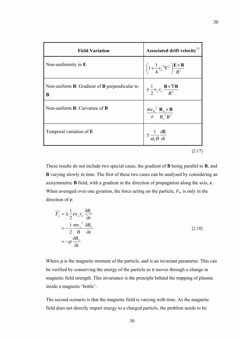
30
Field Variation Associated drift velocity73
Non-uniformity in E 2
22
411
BrL
BE ×⎟⎠⎞
⎜⎝⎛ ∇+
Non-uniform B: Gradient of B perpendicular to
B 22
1B
rv LBB ∇×± ⊥
Non-uniform B: Curvature of B 22
2
BRemv
c
II BR c ×
Temporal variation of E dtd
Bc
Eω
1±
[2.17]
These results do not include two special cases, the gradient of B being parallel to B, and
B varying slowly in time. The first of these two cases can be analysed by considering an
axisymmetric B field, with a gradient in the direction of propagation along the axis, z .
When averaged over one gyration, the force acting on the particle, Fz, is only in the
direction of z:
zB
zB
Bmv
zB
revF
z
z
zLz
∂∂
−=
∂∂
−=
∂∂
±=
⊥
⊥
µ
2
2121
[2.18]
Where µ is the magnetic moment of the particle, and is an invariant parameter. This can
be verified by conserving the energy of the particle as it moves through a change in
magnetic field strength. This invariance is the principle behind the trapping of plasma
inside a magnetic ‘bottle’.
The second scenario is that the magnetic field is varying with time. As the magnetic
field does not directly impart energy to a charged particle, the problem needs to be
31
31
analysed from the electric field associated with the magnetic field as given by
Maxwell’s equation:
dtdBE −=×∇ [2.19]
If we assume the field changes slowly, we can show that the associated electric field
alters the perpendicular velocity. Hence, an increase in the magnetic field strength is
coupled directly into an increased kinetic energy of the particles orbiting around the
guiding centre, varying the Larmor radius. This fact can be used to heat a plasma by
increasing the external magnetic field. This derivation can be extended to show that the
magnetic moment, µ, is also invariant in time.
From this we can conclude that in order to prevent a drift velocity, or related effect
perturbing an experiment performed in a magnetic field, the field must be both spatially
and temporally uniform over the extent of the experiment.
2.2.3 Plasma Oscillations
In the previous section we have seen that that particle orbits can be characterised by the
Larmor radius and gyro-frequency. Oscillations in plasmas have their own characteristic
plasma frequency, ωp.
The plasma frequency can be derived from a consideration of the effects of a small
perturbation in the electron distribution in homogeneous plasma80 such as would be
screened within the Debye length. If the background particle density distribution, n0, is
homogeneous for both ions and electrons the electron density function, ne, can be
written as
),(),( 10 tnntne rr += [2.20]
The perturbation in electron density, n1, will give rise to an electric field proportional to
the size of the perturbation. This will in turn accelerate all the surrounding electrons
(ignoring the ion motion due to their inertia) to a small velocity u . Considering that the
perturbation is much smaller than the background density, the change in the
perturbation leads to a restoring motion in the flow such that:
32
32
u⋅∇−=∂
∂0
1 nt
n [2.21]
Due to the force exerted on the electrons, of mass me, by the electric field
Eu et
me −=∂∂
[2.22]
And the electric field is given by Poisson’s equation
en100
11ε
ρε
==⋅∇ E [2.23]
If the temporal derivative of [2.21] and the divergence of [2.22] are substituted into
[2.23] we obtain
010
20
21
2
=⎟⎟⎠
⎞⎜⎜⎝
⎛−
∂∂ n
men
tn
eε [2.24]
Implying that any electron density perturbation will oscillate with a natural frequency,
called the plasma frequency, ωp given by
ep m
en
0
20
εω = [2.25]
2.3 Collisionality
In order that electromagnetic forces and not collisions dominate the behaviour of
particles, the natural frequency of plasma oscillations ωp has to be greater than the
collision frequency between particles. If the mean time between collisions is τ this
condition becomes:
1>τω p [2.26]
33
33
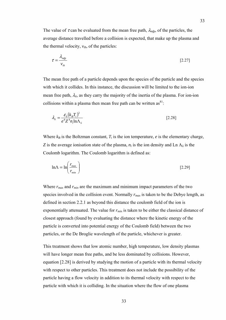
The value of τ can be evaluated from the mean free path, λmfp, of the particles, the
average distance travelled before a collision is expected, that make up the plasma and
the thermal velocity, vth, of the particles:
th
mfp
vλ
τ = [2.27]
The mean free path of a particle depends upon the species of the particle and the species
with which it collides. In this instance, the discussion will be limited to the ion-ion
mean free path, λii, as they carry the majority of the inertia of the plasma. For ion-ion
collisions within a plasma then mean free path can be written as81:
( )ii
44
20
lnΛi
iBii nZe
Tkελ = [2.28]
Where kB is the Boltzman constant, Ti is the ion temperature, e is the elementary charge,
Z is the average ionisation state of the plasma, ni is the ion density and Ln Λii is the
Coulomb logarithm. The Coulomb logarithm is defined as:
⎟⎟⎠
⎞⎜⎜⎝
⎛=
min
maxlnlnΛrr
[2.29]
Where rmax and rmin are the maximum and minimum impact parameters of the two
species involved in the collision event. Normally rmax is taken to be the Debye length, as
defined in section 2.2.1 as beyond this distance the coulomb field of the ion is
exponentially attenuated. The value for rmin is taken to be either the classical distance of
closest approach (found by evaluating the distance where the kinetic energy of the
particle is converted into potential energy of the Coulomb field) between the two
particles, or the De Broglie wavelength of the particle, whichever is greater.
This treatment shows that low atomic number, high temperature, low density plasmas
will have longer mean free paths, and be less dominated by collisions. However,
equation [2.28] is derived by studying the motion of a particle with its thermal velocity
with respect to other particles. This treatment does not include the possibility of the
particle having a flow velocity in addition to its thermal velocity with respect to the
particle with which it is colliding. In the situation where the flow of one plasma
34
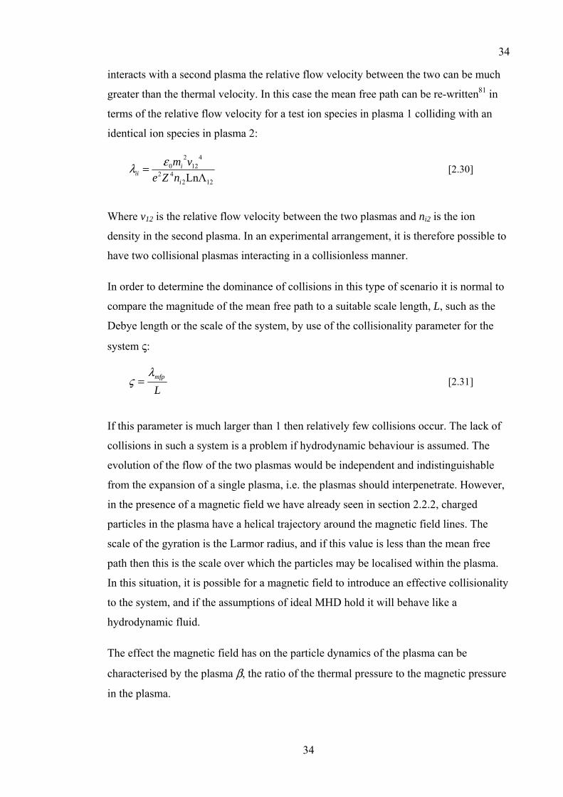
34
interacts with a second plasma the relative flow velocity between the two can be much
greater than the thermal velocity. In this case the mean free path can be re-written81 in
terms of the relative flow velocity for a test ion species in plasma 1 colliding with an
identical ion species in plasma 2:
12242
412
20
LnΛi
iii nZe
vmελ = [2.30]
Where v12 is the relative flow velocity between the two plasmas and ni2 is the ion
density in the second plasma. In an experimental arrangement, it is therefore possible to
have two collisional plasmas interacting in a collisionless manner.
In order to determine the dominance of collisions in this type of scenario it is normal to
compare the magnitude of the mean free path to a suitable scale length, L, such as the
Debye length or the scale of the system, by use of the collisionality parameter for the
system ς:
Lmfpλ
ς = [2.31]
If this parameter is much larger than 1 then relatively few collisions occur. The lack of
collisions in such a system is a problem if hydrodynamic behaviour is assumed. The
evolution of the flow of the two plasmas would be independent and indistinguishable
from the expansion of a single plasma, i.e. the plasmas should interpenetrate. However,
in the presence of a magnetic field we have already seen in section 2.2.2, charged
particles in the plasma have a helical trajectory around the magnetic field lines. The
scale of the gyration is the Larmor radius, and if this value is less than the mean free
path then this is the scale over which the particles may be localised within the plasma.
In this situation, it is possible for a magnetic field to introduce an effective collisionality
to the system, and if the assumptions of ideal MHD hold it will behave like a
hydrodynamic fluid.
The effect the magnetic field has on the particle dynamics of the plasma can be
characterised by the plasma β, the ratio of the thermal pressure to the magnetic pressure
in the plasma.
35
35
202
Bpµβ = [2.32]
Where µ0 is the permeability of vacuum. For the magnetic field to induce an effective
collisionality into the system without affecting the expansion of the two counter-
streaming plasmas would require a judicious choice of magnetic field strength such that
the value of β is much greater than 1, while the Larmor radius is still smaller than the
mean free path and the scale of the system.
2.4 Collisionless shocks
Collisionless shocks are a common astrophysical phenomenon, but not naturally
occurring on earth. Our nearest example of a collisionless shock is the bow shock
around the Earth82 caused by the interaction of the solar wind with the earth’s magnetic
field. In this section, I will explore the formation of a collisionless shock through
developing the standard theory of a hydrodynamic shock and showing how the same
processes can occur in a collisionless system.
2.4.1 Shock formation
If we consider a pressure wave in a perfect gas where the speed of sound, cs, is given by
cs = √(γp/ρ), where p is the pressure, ρ is the density and γ is the adiabatic index. The
variation of pressure along the wave will lead to locally defined regions moving at
different speeds, as the sound speed is a function of pressure. High-pressure elements of
the wave will move faster than the lower-pressure regions causing the waveform to
become steeper. As the velocity of the fluid can only have a single value at any point,
the fluid elements cannot physically overtake each other and eventually a discontinuity
is formed.
If the magnitude of the pressure variation in the wave is small compared to the
background pressure then this can be considered indistinguishable from an acoustic
wave propagating with uniform sound speed. However, for large variations of pressure
a shock is produced.
36
36
What prevents the wave from overturning is the mechanism for momentum transfer and
wave propagation82. If this mechanism is able to balance the processes that steepen the
wave, then a steady shock wave is produced.
2.4.2 Shock conditions
A shock wave is a discontinuity in the pressure and density of a fluid travelling faster
than the local speed of sound. This discontinuity separates the fluid into two regions, the
upstream region into which the shock is propagating and the downstream region
through which the shock has already passed.
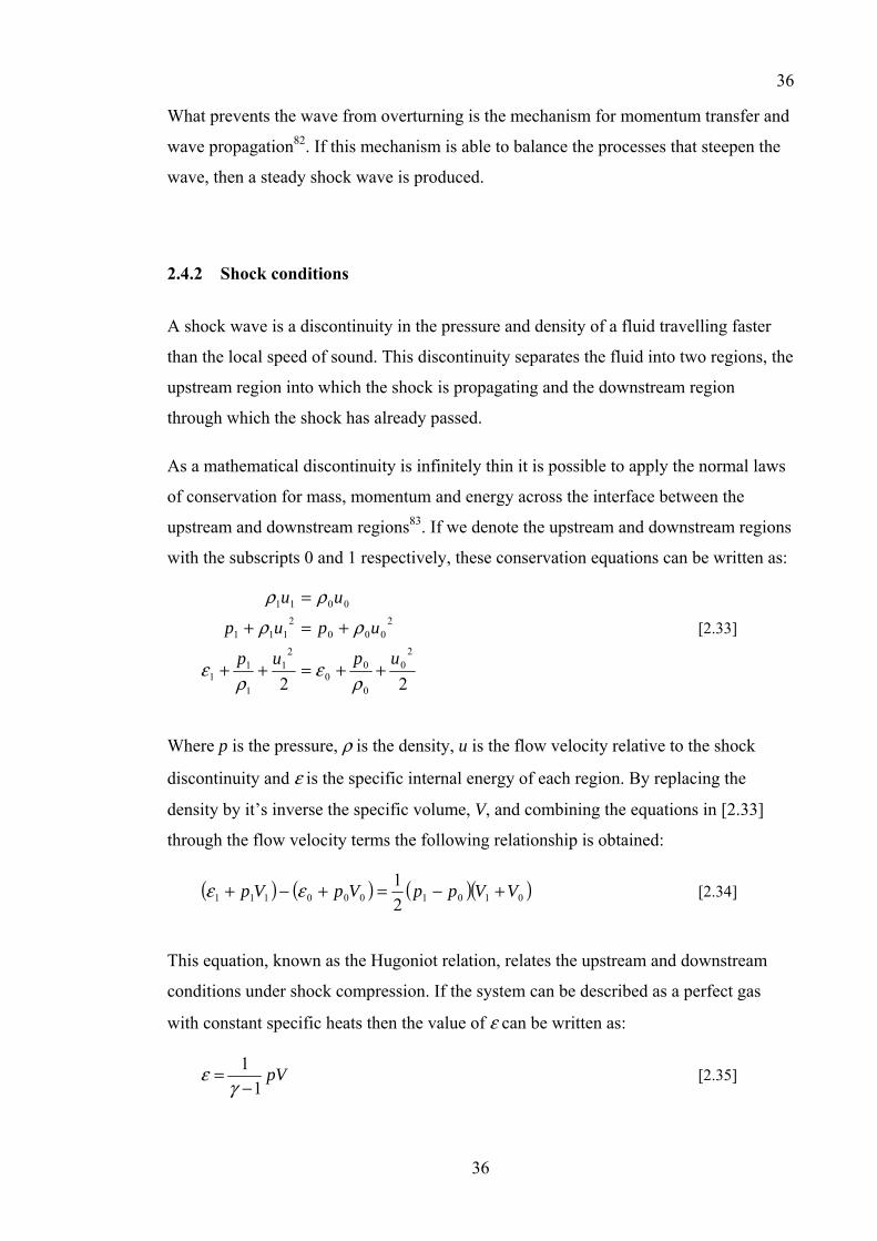
As a mathematical discontinuity is infinitely thin it is possible to apply the normal laws
of conservation for mass, momentum and energy across the interface between the
upstream and downstream regions83. If we denote the upstream and downstream regions
with the subscripts 0 and 1 respectively, these conservation equations can be written as:
22
20
0
00
21
1
11
2000
2111
0011
upup
upup
uu
++=++
+=+
=
ρε
ρε
ρρ
ρρ
[2.33]
Where p is the pressure, ρ is the density, u is the flow velocity relative to the shock
discontinuity and ε is the specific internal energy of each region. By replacing the
density by it’s inverse the specific volume, V, and combining the equations in [2.33]
through the flow velocity terms the following relationship is obtained:
( ) ( ) ( )( )0101000111 21 VVppVpVp +−=+−+ εε [2.34]
This equation, known as the Hugoniot relation, relates the upstream and downstream
conditions under shock compression. If the system can be described as a perfect gas
with constant specific heats then the value of ε can be written as:
pV1
1−
=γ
ε [2.35]
37
37
Where γ is the adiabatic index. This allows an explicit form of the Hugoniot relation to
be written:
( ) ( )( ) ( ) 01
10
0
1
1111
VVVV
pp
−−+−−+
=γγγγ
[2.36]
From this, it can be seen that for a set of initial upstream conditions there is a fixed set
of possible downstream conditions, a locus of end points known as the Hugoniot curve.
This also introduces a limit to the amount of compression that can occur due to the
shock equal to:
11
1
0
0
1
−+==
γγ
ρρ
VV
[2.37]
For an ideal gas, γ is 5/3 implying a maximum compression of a factor of four. The
treatment of the properties of the shock can now be classified into two types, strong
shocks where p1/p0 → ∞ and weak shocks where p1 ≈ p0. In the case of a strong shock,
the degree of compression is near the limit imposed by [2.37]. If we consider the case of
the strong shock then the upstream and downstream flow velocities can be written as:
( )( )
21
01
2
1
21
010
121
21
⎟⎟⎠
⎞⎜⎜⎝
⎛
+−=
⎟⎠⎞
⎜⎝⎛ +=
Vpu
Vpu
γγ
γ
[2.38]
If these velocities are compared with the speed of sound in each region, cs = √(γpV), it
can be shown that:
( ) ( )
( ) ( )γ
γγ
γ
γγ
2
11
2
11
1
02
1
1
0
12
0
0
pp
cu
pp
cu
s
s
++−=⎟⎟
⎠
⎞⎜⎜⎝
⎛
++−=⎟⎟
⎠
⎞⎜⎜⎝
⎛
[2.39]
This shows that the downstream flow is subsonic, whereas the upstream flow is
supersonic, as required by the definition of a shock. The ratio of the upstream flow
38
38
velocity to the speed of sound, termed the Mach number, M, serves as a useful indicator
of the shock strength. For a weak shock M is close to 1, whereas for a strong shock
M>>1.
2.4.3 Shock thickness
In the theoretical treatment of the previous section the shock discontinuity is considered
to be infinitely thin, however in a real shock the transition must occur over a finite
layer. As there is a change in entropy between the upstream and downstream region, a
dissipative mechanism must be responsible for the transition. The dissipative
mechanism is responsible for defining the width of the transitional region in terms of
the characteristic scale length of the mechanism involved to heat the fluid experiencing
the compression. For a fluid where the dominant mechanism for heat transfer is through
binary collisions the characteristic scale length would be the mean free path of the
particles.
However, for a shock to form in a collisionless plasma where binary collisions are rare,
a different form of dissipative mechanism must be dominant. The processes leading to
the wave steepening in a collisionless plasma are more complex than the treatment in
section 2.4.1. A collisionless plasma is a dispersive media, which means that the speed
of the wave propagation is a function of the wavelength, as determined by a dispersion
relation. A derivation of a basic plasma dispersion relation is given in Chapter 3,
however for the purposes of this treatment the relevant dispersion relation is such that
for wavelengths above a critical value the wave velocity is constant. Below the critical
value the wave velocity either increases or decreases with wavelength, depending on the
orientation of the wave propagation to the magnetic field.
If we consider again the concept of a steepening wave, but in this instance, decompose
the wave into its Fourier components. As the wave becomes steeper the short
wavelength Fourier components become more dominant in the series. As the different
wavelength components below the critical value now have different velocities due to
dispersion, the dominant components will physically separate themselves from the bulk
of the wave. The cyclic combination of steepening, dispersion and separation converts
the initial wave into a series of pulses of thickness approximately that of this critical
wavelength. The magnetic field defines a unique direction with respect to the shock. In

39
39
general, there are three orientations of the magnetic field with respect to the flow of the
fluid: perpendicular, parallel and the general case of at an angle. In our experiment, the
magnetic field is perpendicular to the flow of the fluid.
When the magnetic field is perpendicular to the propagation of the wave, the dispersion
relation84 decreases the wave velocity for wavelengths below c/ωp, producing a series of
compression pulses. As the weakest (lowest amplitude) pulses are produced first and
subsequently fall behind the bulk of the wave, the shock front will take the form of a
large pulse followed by a series of pulses of decreasing amplitude. In a collisionless
perpendicular shock, the type of wave involved is a magneto-acoustic wave, with a
characteristic Alfvén velocity85 analogous to the speed of sound in an acoustic wave. In
this regime, it is more appropriate to consider the shock conditions in terms of the ratio
of the flow velocity to the Alfvén velocity, termed the Alfvén Mach number, MA .
When the magnetic field is not perpendicular to the propagation direction, the
dispersion relation will increase the wave velocity for wavelengths below the ion
Larmor radius82. This produces a shock front comprised of a wave train of rarefaction
pulses of increasing amplitude.
The thickness of the shock is now governed by the length of the wave train of pulses,
which in turn is governed by the rate at which the energy of these pulses dissipates.
The possible mechanisms for collisionless dissipation of the wave train again depend on
the orientation of the wave propagation to the magnetic field, and in some cases the
strength of the shock itself. Descriptions of proposed collisionless dissipative
mechanisms, from wave-particle interactions to magnetic turbulence can be found in the
literature 68,82,84,86. A complete treatment of all the possible types of dissipation would
be beyond the scope of this chapter, as the important parameter is the scale length of the
dissipative mechanism, which has already been discussed. If whatever mechanism is
employed is sufficient to balance the entropy difference between the upstream and
downstream regions, it will be achieved on a scale comparable with the size of the
pulses. Hence for a perpendicular shock we would expect the shock thickness to be of
the order of c/ωp, and for a non perpendicular shock we would expect the thickness to
be of the order of the ion Larmor radius.
40
40
Our closest example of a collisionless shock is the bow shock formed by the solar wind
around the Earth’s magnetic field. The thickness of this shock is around 103km whereas
the mean free path of the solar wind is approximately 108km. It is worth noting that in
the region of the shock the magnetic field is between 45 to 50 degrees to the shock
front, and the ion Larmor radius is several hundred kilometres82. Furthermore, the
system has a low plasma β~1, whereas for our system of interest, a 100 year old SNR,
β>>1. The observed shock thickness is very close to the scale length of shock thickness
predicted for a non-perpendicular shock.
2.5 Scaling
From the derivations in the previous sections, we can deduce several important plasma
parameters. These parameters, such as the Debye length, plasma frequency and Larmor
radius, yield scales over which we can infer the behaviour of the plasma to be governed
in a certain way. However, if we wish to compare the behaviour of two different
plasmas we need to introduce the concept of scale invariance.
Scaling laws rely on the use of dimensionless constants relevant to the two systems If
the assumptions of the scaling model hold, then the two systems will show similarity.
For example, if we consider the basic example of a rectangle of sides length a and b . If
we wish to compare this rectangle with another rectangle of sides length a’ and b’, only
if the dimensionless ratio a/b was the same as a’/b’ would the two rectangles be similar.
It can also be seen from this treatment that there exists a scaling transformation between
the two systems which satisfies the matching of the dimensionless constant, namely that
a’ = xa and b’ = xb, a linear transformation of magnification x.
This principle was extended by Connor and Taylor87 to show that if the fundamental
equations describing plasma behaviour are invariant under a given transformation, then
a scaling law derived from those equations must also be invariant under the
transformation. To apply an invariant scale there are constraints placed on the model
used to describe the plasma. Our aim is to create a simulation of a SNR and scale such
an experiment using an argument. The SNR phenomenon is a collisionless, high β
system to which ideal MHD can be applied. Connor and Taylor87 identified an ideal
MHD transformation which they termed ‘E2’. This transformation seems the most
appropriate to seek in experiments.
41
41
Ryutov et al88 developed these concepts further, and propose a set of transformations
for the Euler equations describing the evolution of an ideal compressible hydrodynamic
fluid with the thermodynamic properties of a polytropic gas. This work was later
extended89 to the case of ideal MHD. In this case the Euler equations are:
0=•∇+∂∂ vρρ
t [2.40]
BBvvv ××∇+−∇=⎟⎠⎞
⎜⎝⎛ ∇•+
∂∂ )(1
0µρ p
t [2.41]
BvB ××∇=∂∂
t [2.42]
Where v is the velocity, ρ is the density, p is the pressure and B is the magnetic field.
These equations describe conservation of mass, conservation of momentum and
magnetic induction respectively. A fourth equation, for conservation of energy is also
required:
( ) vv •∇+−=∇•+∂∂ εεε p
t [2.43]
Where ε is the internal energy per unit volume. As the system is described as a
polytropic gas, the internal energy is a linear function of the pressure:
Cp=ε [2.44]
The assumption of a polytropic gas is suitable for describing a fully ionised medium, as
there are no changes in the number of degrees of freedom caused by an increase in
temperature. Substituting [2.44] into [2.43] leads to:
vv •∇−=∇•+∂∂ pp
tp γ [2.45]
Where γ is the adiabatic index equal to 1 + 1/C.
These equations are invariant under the transformations between systems 1 and 2
denoted with subscripts:
42
42
21
21
21
21
21
21
BB
vv
ccb
tcbat
cppbarr
=
=
=
===
ρρ
[2.46]
Where a, b, and c are arbitrary positive numbers. For these transformations Ryutov et
al89 demonstrate the invariance of two dimensionless parameters from an initial value
problem for the similarity of two evolving plasmas:
2
2
1
1
2
22
1
11
pp
Eupp
BB
vv
=
==ρρ
[2.47]
The first invariant, Eu, dubbed the Euler number by Ryutov et al, and when calculated
the velocities, pressures and densities do not have to all be taken from the same point.
However, the values must be taken from corresponding points in both systems. The
second invariant is equivalent to the inverse of the square root of the plasma β, which
has already been defined as a key dimensionless parameter for scaling by Connor and
Taylor87.
This derivation makes a number of assumptions about the plasma, the validity of which
needs to be examined. The primary assumption of any fluid description is that the
medium involved can be treated as a fluid. In the case of a collisionless interaction as
described in section 2.3, this may not always be the case. However, assuming an
external magnetic field is applied to the plasma of sufficient strength that the Larmor
radius is smaller than the mean free path and the system size, then this assumption is
valid.
This treatment assumes gravitational effects are negligible as this force is not included
in any form, which is valid for the laboratory experiment, but may not be for an
astrophysical plasma.
43
43
By describing the plasma by the Euler equations the effects of heat conduction,
viscosity and radiative diffusion are all assumed to be negligible as the treatment does
not include the effects of dissipative terms.90 The use of ideal MHD also implicitly
assumes that the fluid has zero resistivity.91
The scaling argument presented by Ryutov et al is designed to show that two systems
with identical initial conditions will evolve in a similar manner if the scaling conditions
are met. However, it is not always possible to duplicate the initial conditions of an
astrophysical system of interest. In this scenario, we present the assumption that if a
laboratory simulation can evolve to a point where the similarity criteria are met, then for
a limited time the behaviour of the two systems may be similar. This should enable a
‘snapshot’ of the system to be created, suitable for testing the physics of the
astrophysical system in the laboratory.
Hence we have two scaling parameters which we need to match in any experiment, Eu
and β, but there are other factors to consider. In the simulation we are trying to achieve,
a collision-free interaction is required, so the collisionality, ς, needs to be much greater
than 1. We also require a high Alfven mach number, MA, shock, hence this parameter
should be much greater than 1.
In considering the design of an experiment to match these scaling criteria, it is useful to
compare the range of plasma parameters that are observed from different sources. The
table below presents a comparison between the conditions typical of naturally occurring
plasmas and the conditions typical of laboratory produced plasmas. Included in the table
are values for magnetic confinement fusion experiments (MFE) and inertially confined
fusion experiments (IFE).
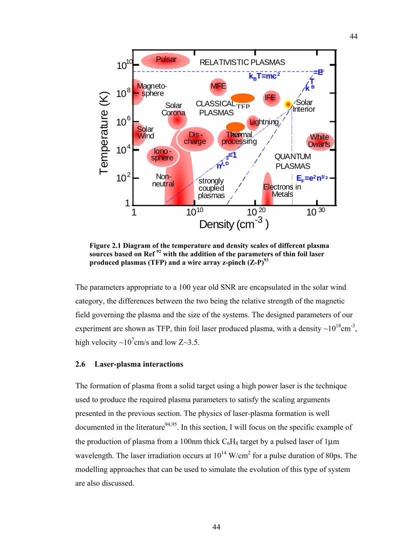
44
44
RELATIVISTIC PLASMAS
QUANTUMPLASMAS
CLASSICALPLASMAS
stronglycoupledplasmas
Pulsar
MFEIFE
SolarCorona
Dis -charge
Iono -sphere
SolarWind
Magneto-sphere
Non-neutral
Thermalprocessing
Lightning
WhiteDwarfs
Electrons inMetals
SolarInterior
kBT=mc2
k BT=EF
EF=e2n1/ 3
nλD3=1
1010
108
106
104
102
1
Tem
pera
ture
(K)
1 1010 10 20 10 30
Density (cm-3 )
Figure 2.1 Diagram of the temperature and density scales of different plasma sources based on Ref 92 with the addition of the parameters of thin foil laser produced plasmas (TFP) and a wire array z-pinch (Z-P)93
The parameters appropriate to a 100 year old SNR are encapsulated in the solar wind
category, the differences between the two being the relative strength of the magnetic
field governing the plasma and the size of the systems. The designed parameters of our
experiment are shown as TFP, thin foil laser produced plasma, with a density ~1018cm-3,
high velocity ~107cm/s and low Z~3.5.
2.6 Laser-plasma interactions
The formation of plasma from a solid target using a high power laser is the technique
used to produce the required plasma parameters to satisfy the scaling arguments
presented in the previous section. The physics of laser-plasma formation is well
documented in the literature94,95. In this section, I will focus on the specific example of
the production of plasma from a 100nm thick C6H8 target by a pulsed laser of 1µm
wavelength. The laser irradiation occurs at 1014 W/cm2 for a pulse duration of 80ps. The
modelling approaches that can be used to simulate the evolution of this type of system
are also discussed.
TFP
Z-P
45
45
Initially the laser is incident on the surface of the solid target, and the high average
electric field (~2.7x10¹⁰ V/m in vacuum) removes electrons from the solid surface over
a period of a few laser cycles96. These electrons are further accelerated by the electric
field and will cause ionisation through collisions with the solid. This will produce
mobile ions, which expand into the vacuum. After approximately 10-12s a plasma has
been formed with an roughly exponential density profile decaying away from the solid
surface. The laser is now interacting with a plasma, which has its own natural response
frequency to electric field perturbations, the plasma frequency as defined in section
2.2.1. The effect of the plasma natural frequency is to place an upper limit on the
density of the plasma to which the laser light can penetrate. At this point the frequency
of the laser beam matches the electron plasma frequency. The electron density at which
this occurs is termed the critical density, nc. As will be discussed in the next chapter, the
refractive index of the plasma at this point falls to zero. A useful formula for calculating
the value of the critical density for any wavelength is:
[ ] [ ]2
213
µm101.1cm
λ×=−
cn [2.49]
Where λ[µm] is the wavelength of the laser in µm and nc[cm-3] is the critical density in
cm-3. For a 1µm laser, the critical density surface is at 1.1x1021cm-3, two orders of
magnitude below solid density at around 1023cm-3.
At the intensity of 1014 W/cm2, the laser energy is mostly absorbed in the under-dense
(below critical density) region of the plasma through a process known as inverse
bremsstrahlung. Bremsstrahlung radiation can be considered as the emission of
radiation by an electron undergoing acceleration in the field of an ion97. Hence, inverse
bremsstrahlung can be considered to be the absorption of a photon during the collision
of an electron with an ion. The absorption coefficient for this process, αib, can be
written as96:
22
2
ωω
α+
=ei
peiib vnc
v [2.50]
46
46
Where n is the refractive index, c is the speed of light in vacuum, ω is the angular
frequency of the laser, ωp is the plasma frequency and vei is the electron-ion collision
frequency given by:
gZen
Tkmv e
eBeei 3
12
161
20
423
21
πεππ ⎟⎟
⎠
⎞⎜⎜⎝
⎛⎟⎟⎠
⎞⎜⎜⎝
⎛= [2.51]
Where Z is the ionisation state, ne the electron density, kB the Boltzman constant, Te is
the electron temperature, me is the mass of an electron and g is the Gaunt factor ~1.
From this, we can see that the rate of absorption is going to increase with plasma
density, and that the absorption is most efficient for cold electrons. Once the electrons
become heated, the collision frequency will decrease and the electrons will remain at a
fixed temperature, but be collisionless with respect to the ions.
Diffusive transport by the heated electrons into the over-dense plasma propagates the
laser energy to the solid surface where the solid is ablated to form more plasma. The
lower energy particles produced at the ablation front drift back to the under-dense
region where they are heated and the process cycles. In thick targets the pressure of the
ablation process can form a shock wave that compresses the target, however in thin foils
the entire target is completely ablated before a shock would be able to develop.
Once the foil has been completely ablated, the plasma is heated for the remainder of the
laser pulse. After the laser has been switched off, the plasma’s behaviour can be
modelled as an adiabatic expansion98.
By treating the plasma as a single fluid, the adiabatic expansion can be modelled from
the ideal hydrodynamic equations in one dimension99:
( )
xxvv
tv
xv
t
∂∂−=⎟
⎠⎞
⎜⎝⎛
∂∂+
∂∂
=∂
∂+∂∂
ρρ
ρρ 0 [2.52]
Where ρ is the density, p is the pressure and v is the velocity of the fluid. If we assume
that the plasma is uniformly heated and that the instantaneous velocity is going to be a
linear function of position based on a time-dependent scale factor, L:
47
47
xLdt
dLv
⎟⎟⎟
⎠
⎞
⎜⎜⎜
⎝
⎛= [2.53]
For each instant, the density function will take the form of a Gaussian distribution:
( ) ⎥⎦
⎤⎢⎣
⎡−= 2
2
)(2exp
)(1,
tLx
tLtxne [2.54]
Where for a given time the value of the scale factor L can be found from the speed of
sound in the plasma, cs, and the original width of the foil L0:
⎟⎟⎠
⎞⎜⎜⎝
⎛⎟⎟⎠
⎞⎜⎜⎝
⎛=
0
ln2LL
cLt
s
[2.55]
This analytical model can be extended further99 to include the rate of heating during the
laser pulse and the heating of the plasma after the plasma has expanded to below critical
density. However, as in the case of the 80ps laser pulse we are considering it should
take ~250ps for the plasma to become under-dense.
More detailed modelling of the production of thin foil plasma can be achieved through
the use of numerical simulations. For the conditions already outlined, we utilised a
modified version of the simulation code Medusa100. This is a one dimensional
lagrangian numerical simulation of the hydrodynamic and thermodynamic behaviour of
a plasma irradiated by an intense laser. The modifications made to Medusa for these
simulations allow the plasma to expand to a fixed point in vacuum where it reaches a
barrier. In addition, the code was modified by R.G. Evans to include flux limited
thermal conductivity, required for shock simulation. In this way, the single fluid code
should be able to model the two extreme cases of a counter propagating plasma system.
Firstly, if the system is completely collisionless, yet a fluid description can be applied,
the evolution of one plasma should be independent of the presence of the second
plasma, hence only one plasma needs to be modelled. Secondly, if the plasmas cannot
interpenetrate then the evolution of each plasma should be self-contained up to the
halfway point between the two plasmas.
48
48
A series of numerical investigations into possible experimental configurations were
carried out101 to find a suitable experimental geometry for producing conditions suitable
for matching the scaling criteria. The experimental design is based on the conditions
considered in this section, the production of plasma from two 100nm thick C6H8 targets
by 1µm laser irradiation at 1014 W/cm2 with a gaussian 80ps pulse. The foils are placed
face parallel in a counter-propagating geometry with a separation of 1mm. To ensure the
one-dimensional treatment of the expansion is valid, experimentally a 1mm diameter
focal spot is required. The results of the experimental simulations are presented
below102:
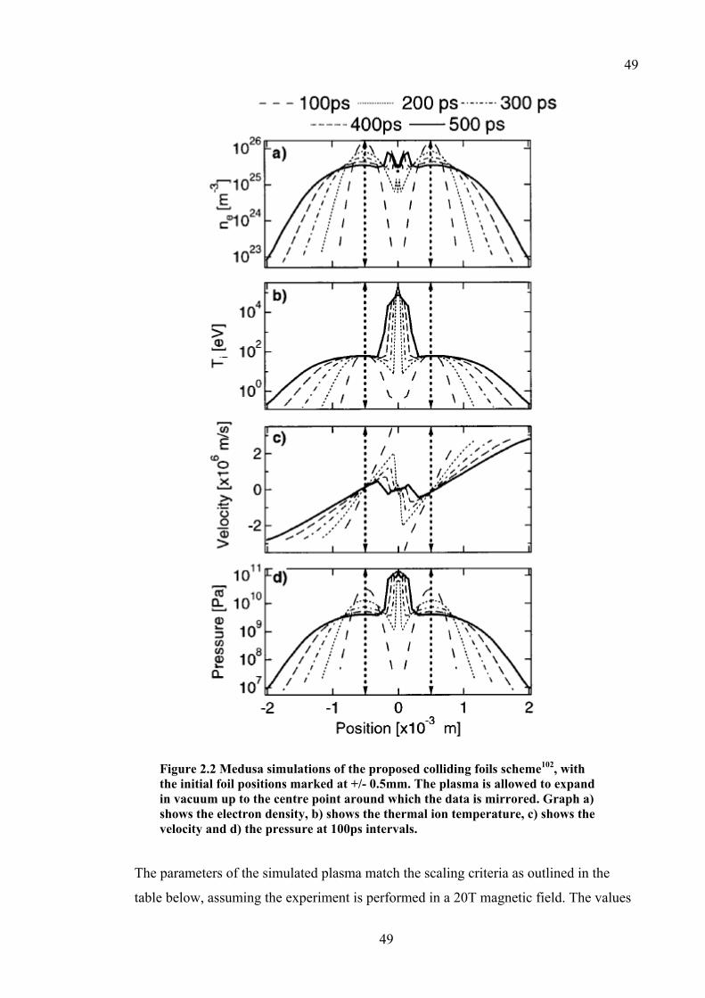
49
49
Figure 2.2 Medusa simulations of the proposed colliding foils scheme102, with the initial foil positions marked at +/- 0.5mm. The plasma is allowed to expand in vacuum up to the centre point around which the data is mirrored. Graph a) shows the electron density, b) shows the thermal ion temperature, c) shows the velocity and d) the pressure at 100ps intervals.
The parameters of the simulated plasma match the scaling criteria as outlined in the
table below, assuming the experiment is performed in a 20T magnetic field. The values
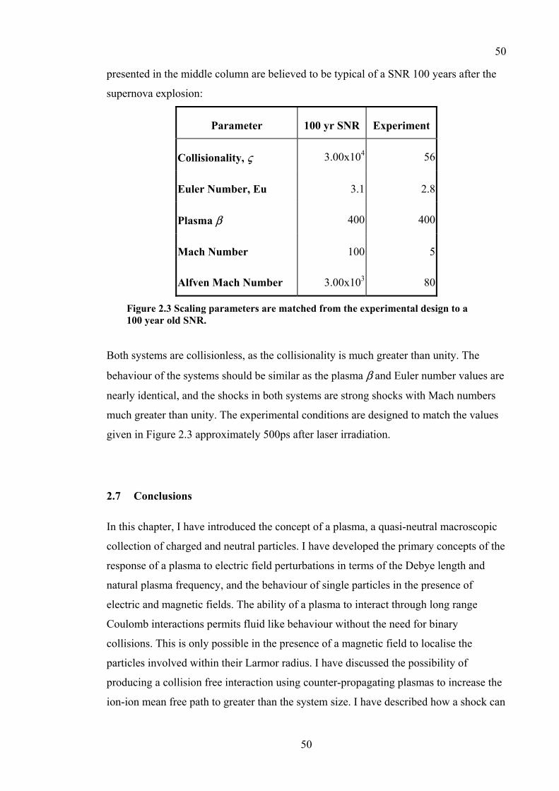
50
50
presented in the middle column are believed to be typical of a SNR 100 years after the
supernova explosion:
Parameter 100 yr SNR Experiment
Collisionality, ς 3.00x10⁴ 56
Euler Number, Eu 3.1 2.8
Plasma β 400 400
Mach Number 100 5
Alfven Mach Number 3.00x10³ 80
Figure 2.3 Scaling parameters are matched from the experimental design to a 100 year old SNR.
Both systems are collisionless, as the collisionality is much greater than unity. The
behaviour of the systems should be similar as the plasma β and Euler number values are
nearly identical, and the shocks in both systems are strong shocks with Mach numbers
much greater than unity. The experimental conditions are designed to match the values
given in Figure 2.3 approximately 500ps after laser irradiation.
2.7 Conclusions
In this chapter, I have introduced the concept of a plasma, a quasi-neutral macroscopic
collection of charged and neutral particles. I have developed the primary concepts of the
response of a plasma to electric field perturbations in terms of the Debye length and
natural plasma frequency, and the behaviour of single particles in the presence of
electric and magnetic fields. The ability of a plasma to interact through long range
Coulomb interactions permits fluid like behaviour without the need for binary
collisions. This is only possible in the presence of a magnetic field to localise the
particles involved within their Larmor radius. I have discussed the possibility of
producing a collision free interaction using counter-propagating plasmas to increase the
ion-ion mean free path to greater than the system size. I have described how a shock can
51
51
form in such a collisionless system, including the characteristic shock thickness that
would be expected to form. I have introduced the scaling laws relevant to a plasma
which can be described by ideal MHD.
I have demonstrated how a plasma can be produced from a thin foil by laser irradiation,
and the parameters of such a plasma can be modelled by analytical and numerical
methods. I have also shown that the parameters of a laser-plasma experiment can be
designed to be similar to a 100 year old SNR.
52
52
3 Chapter 3 - Optical probes.
3.1 Introduction
This chapter is a review of the properties of optical laser probes, and how these probes
can be used to measure parameters such as the refractive index of a plasma. The
interaction of a laser probe with a plasma can be divided in to two categories, a)
scattering processes through the interaction of an electromagnetic wave with a particle,
and b) beam propagation through a plasma. The former processes, which are not of
interest to the work described in this thesis, include Thomson, Mie, Rayleigh, Raman,
and Brillouin scattering103, which represent an extremely useful array of diagnostics.
The latter processes include reflection, transmission, refraction, polarisation, scattering,
and absorption.
The experiments described in Chapters 5 and 6 use a probe in transmission. These
experiments are designed to take advantage of the non-perturbative, accurate, and
sensitive nature of an optical probe to produce space and time resolved data. There are
constraints on the use of a probe set by the probe wavelength, and the spatial resolution
and dynamic range and resolution of the detector. The experiments are designed around
these constraints using computer simulation to determine both the experimental size and
expected electron densities. In these experiments, the probe was used to measure a
number of parameters simultaneously, these are:
1. image of the experiment
2. electron density, ne,
3. electron density gradients, ∇ne, and
4. magnetic field, B
To demonstrate how these measurements can be made, and the underlying assumptions
required I will discuss the propagation of a probe beam through an inhomogeneous
plasma. This description begins with a discussion of the dispersion relation and
refractive index of an ideal plasma to illustrate the conditions for which this treatment is
valid. I will then use the geometrical optics approximation and treat the probe

53
53
propagation in terms of rays and consider a plasma of varying refractive index. This sets
the foundation for describing the design factors necessary in building an optical probe
beam line and imaging system. A number of different probe designs and imaging
systems have been used in experiments, the design specifications and the advantages
and disadvantages are described.
3.2 Theory of propagation of light in an under-dense plasma
In general the passage of an electromagnetic ray through a gas or plasma is affected by
all the scattering, and beam propagation processes mentioned in Section 3.1 and are
illustrated in Figure 3.1. Generally, scattering is observed either at high intensities or
from a large plasma, since scattering cross-sections tend to be very small. The laser
intensities are low, below the damage threshold of delicate optical components
(approximately 0.5 J.cm-2), and the plasma volume and density low, thus scattering is
ignored.
Figure 3.1 Illustration of the processes that occur during the propagation of a laser probe through a plasma. With absorption, these processes tend to attenuate the transmitted beam.
In this Section dispersion and the refractive index of a plasma is described and the
geometrical optics approximation introduced.
Refraction
Scattering
Reflection Transmission Plasma
54
54
3.2.1 The refractive index of a plasma
The effects of a plasma on an electromagnetic wave propagating through it can be
described using the dispersion relation, and its representation as the refractive index, n.
For the derivation of the dispersion relation for an arbitrary plasma with any magnetic
field the reader is directed to the literature where it is well documented 104,105. In this
section I will focus on the simple case of a homogeneous cold plasma and then illustrate
how the more complex the problem of inhomogeneous plasma is treated. The treatment
will be sufficient to develop solutions applicable to the experimental situations
encountered in this research.
If we consider the plasma to be a continuous conducting media then, the propagation of
an electromagnetic wave must satisfy the relevant Maxwell’s equations: -
t
t
∂∂+=×∇
∂∂−=×∇
EjB
BE
000 εµµ [3.1]
Where E is the electric field intensity vector, B is the magnetic induction vector, µ0 is
the permeability of vacuum, ε0 is the permittivity of vacuum, and j is the total current
density. If we eliminate B from the equations, we get
( ) 0000 =⎟⎠⎞
⎜⎝⎛
∂∂+
∂∂+×∇×∇
ttEjE εµµ [3.2]
By using the vector identity:
EEE 2)()( ∇−•∇∇=×∇×∇ [3.3]
By decomposing the electric field into it’s Fourier components, with k as the wave
number and ω is the angular frequency we obtain: -
∫ −•= ωω ω ddt ti kkExE xk 3)(exp),(),( [3.4]
Then we can analyse each Fourier mode E(k,ω) separately and assume the solution to
be valid for all modes. If we re-write [3.2] using [3.4] for a single Fourier mode, and we
obtain
55
55
0)()(
0)()(
0002
000
=++−•
=++××
EjEkEkk
EjEkk
ωµεµωωµεµω
ii
ii [3.5]
As we know the wave we are investigating is transverse we can state that
0=• Ek [3.6]
Also by substituting for the relation
00
2 1µε
=c [3.7]
We get the result
jEk
EjEk
0
222
2
2
0
2
)(εωω
ωεω
ic
ci
−=−
−= [3.8]
If we consider that the current, j, in the plasma is entirely due to electron motion with
electron velocity ve and electron density ne we can write
evj ene−= [3.9]
Where e is the elementary charge. From the equation of motion for an electron
accelerated by an electric field we can also write
ωe
e
ime
tme
Ev
vE
e
e
=
∂∂
= [3.10]
Where me is the mass of an electron. If we substitute this into [3.9] and then [3.8] we get
2222
2
0
2222
2
)(
p
pe
e
e
e
c
menc
imen
ωω
ωε
ω
ω
=−
==−
−=
k
EEEk
Ej
[3.11]

56
56
This is the simple dispersion relation for non-magnetised plasma, which yields the
refractive index n, and introduces the plasma frequency ωp.
2
2
1ωω
ωpcn −== k
[3.12]
However, we are interested in the refractive index as a function of the electron density,
ne. Hence if we define a critical value for the electron density nc such that at nc, ω =ωp
then we can re-write equation 3.12 as
c
e
ec
nnn
emn
−=
=
1
20
2εω
[3.13]
This result is valid for both uniform non-magnetised media but also for a non-
homogeneous magnetised media if a few constraints are satisfied. Firstly the
assumptions required for a non-homogeneous media require that the properties of the
plasma vary slowly enough that the change over one wavelength is negligible, i.e. that
the local conditions surrounding the wave can be considered uniform. This is called the
WKB (Wentzel, Kramers and Brillouin), WKBJ (and Jeffreys), eikonal or geometrical
optics approximation. In all cases the assumption is:
12 <<∇k
k [3.14]
In this situation the homogeneous relation stands locally and can be integrated over the
ray path. This is equivalent to assuming the wavelength of light is negligibly small.
The constraint for the relations to hold to a first order approximation in a magnetised
plasma is that the direction of the ray propagation is parallel with the direction of the
magnetic field vector. The derivation of a more complete dispersion relation will be
treated later in chapter 4 where polarimetry is described Section 4.4.

57
57
3.2.2 Propagation of light in geometrical optics approximation
If the geometrical optics approximation, the assumption that the wavelength of light, λ,
is negligible, produces reliable results for the propagation of a ray of light, then it is
possible to derive the ray path purely from knowledge of the refractive index through
which the ray passes. This is the principal assumption made here, and the approach uses
Maxwell’s equations in the limit that λ→0.106 The resulting equation is commonly
called the eikonal equation, the basic equation of geometrical optics, and is written as
( ) 22 n=∇ζ [3.15]
Where ζ(x,y,z) is the eikonal function or the ‘optical path’, this a scalar function of
position. The eikonal function is the trajectory orthogonal to the geometrical wave
fronts. The route taken by a ray propagating in the medium of refractive index n can be
deduced as a solution such that ζ = constant. If the position vector r of a point on the
ray path can be described as a function of a length of arc s along the ray path then [3.15]
can be re-written as
sr
ddn=∇ζ [3.16]
However this still specifies the ray path in terms of ζ, which is not defined elsewhere.
On differentiating [3.16] with respect to s we can obtain a solution only in terms of the
refractive index n.
( )
( )
( )
( )[ ]2
2
21
21
1
nn
n
n
dddd
ddn
dd
∇=
∇∇=
∇∇•∇=
∇∇•=
∇=⎟⎠⎞
⎜⎝⎛
ζ
ζζ
ζ
ζ
srss
rs
[3.17]

58
58
Which simplifies to:
nddn
dd ∇=⎟
⎠⎞
⎜⎝⎛
sr
s [3.18]
For a homogeneous media, where n is constant (i.e. ∇n= 0) this reduces again to the
solution:
02
2
=sr
dd
[3.19]
This indicates the curvature is zero and a straight-line path obtained as expected. If the
media has a linearly varying refractive index in one direction, say along the x-axis,
defined by a constant α, then the refractive index is:
xx
ˆ0
αα
=∇+=
nnn
[3.20]
From equation 3.18 the ray path is given as
xs
rxs ˆ)ˆ(
2
2
αα =•dd
[3.21]
This implies a parabolic trajectory in the direction of the increase in refractive index.
3.3 The Vulcan Laser System
The probes described in this chapter were all constructed to use beams provided by the
VULCAN laser107 at the Rutherford Appleton Laboratory.
The VULCAN laser is a Master-Oscillator Power Amplifier (MOPA) high power
Nd:Glass laser with 8 separate beamlines. These beams are divided into six 108mm
diameter beams and two 150mm diameter backlighter beams. In these experiments the
beams are all derived from the same oscillator to remove any timing jitter on a shot to
shot basis. The seed pulse is 80ps FWHM formed by a YAG oscillator every 9 seconds.
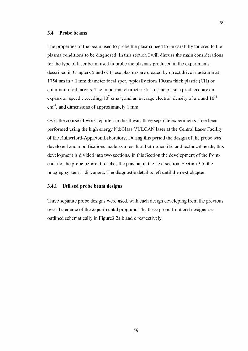
59
59
3.4 Probe beams
The properties of the beam used to probe the plasma need to be carefully tailored to the
plasma conditions to be diagnosed. In this section I will discuss the main considerations
for the type of laser beam used to probe the plasmas produced in the experiments
described in Chapters 5 and 6. These plasmas are created by direct drive irradiation at
1054 nm in a 1 mm diameter focal spot, typically from 100nm thick plastic (CH) or
aluminium foil targets. The important characteristics of the plasma produced are an
expansion speed exceeding 107 cms-1, and an average electron density of around 1018
cm-3, and dimensions of approximately 1 mm.
Over the course of work reported in this thesis, three separate experiments have been
performed using the high energy Nd:Glass VULCAN laser at the Central Laser Facility
of the Rutherford-Appleton Laboratory. During this period the design of the probe was
developed and modifications made as a result of both scientific and technical needs, this
development is divided into two sections, in this Section the development of the front-
end, i.e. the probe before it reaches the plasma, in the next section, Section 3.5, the
imaging system is discussed. The diagnostic detail is left until the next chapter.
3.4.1 Utilised probe beam designs
Three separate probe designs were used, with each design developing from the previous
over the course of the experimental program. The three probe front end designs are
outlined schematically in Figure3.2a,b and c respectively.
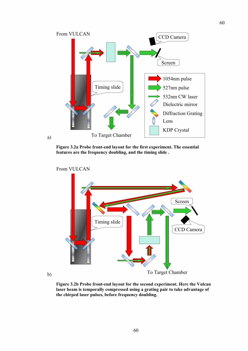
60
60
a)
1054nm pulse
527nm pulse
532nm CW laserDielectric mirror
KDP Crystal
Timing slide
Screen
CCD Camera
To Target Chamber
From VULCAN
Diffraction GratingLens
Figure 3.2a Probe front-end layout for the first experiment. The essential features are the frequency doubling, and the timing slide .
b)
Timing slide
Screen
CCD Camera
To Target Chamber
From VULCAN
Figure 3.2b Probe front-end layout for the second experiment. Here the Vulcan laser beam is temporally compressed using a grating pair to take advantage of the chirped laser pulses, before frequency doubling.

61
61
Timing slide
Screen
CCD Cameras
From VULCAN
Beamsplitter
Variable aperture
c)
Glan-Taylor Polariser
To Target Chamber
750mm EFL
750mm EFL
200 micron pinholeVacuum Chamber
Figure 3.2c Probe front end layout for the third experiment. In addition to pulse compression, frequency doubling, this design uses a vacuum spatial filter (VSF) as the last optical component before entering the vacuum chamber. The VSF is essential to improving the probe near field.
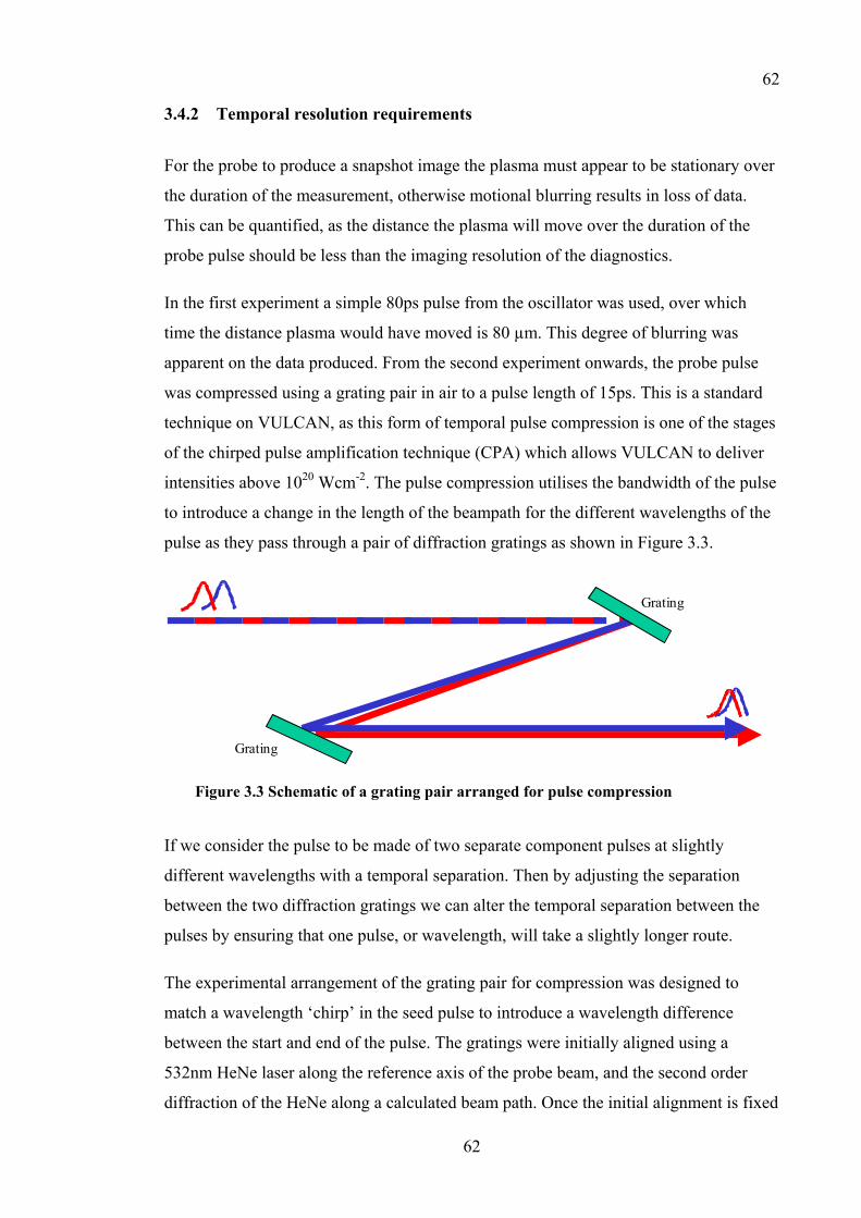
62
62
3.4.2 Temporal resolution requirements
For the probe to produce a snapshot image the plasma must appear to be stationary over
the duration of the measurement, otherwise motional blurring results in loss of data.
This can be quantified, as the distance the plasma will move over the duration of the
probe pulse should be less than the imaging resolution of the diagnostics.
In the first experiment a simple 80ps pulse from the oscillator was used, over which
time the distance plasma would have moved is 80 µm. This degree of blurring was
apparent on the data produced. From the second experiment onwards, the probe pulse
was compressed using a grating pair in air to a pulse length of 15ps. This is a standard
technique on VULCAN, as this form of temporal pulse compression is one of the stages
of the chirped pulse amplification technique (CPA) which allows VULCAN to deliver
intensities above 1020 Wcm-2. The pulse compression utilises the bandwidth of the pulse
to introduce a change in the length of the beampath for the different wavelengths of the
pulse as they pass through a pair of diffraction gratings as shown in Figure 3.3.
Grating
Grating
Figure 3.3 Schematic of a grating pair arranged for pulse compression
If we consider the pulse to be made of two separate component pulses at slightly
different wavelengths with a temporal separation. Then by adjusting the separation
between the two diffraction gratings we can alter the temporal separation between the
pulses by ensuring that one pulse, or wavelength, will take a slightly longer route.
The experimental arrangement of the grating pair for compression was designed to
match a wavelength ‘chirp’ in the seed pulse to introduce a wavelength difference
between the start and end of the pulse. The gratings were initially aligned using a
532nm HeNe laser along the reference axis of the probe beam, and the second order
diffraction of the HeNe along a calculated beam path. Once the initial alignment is fixed
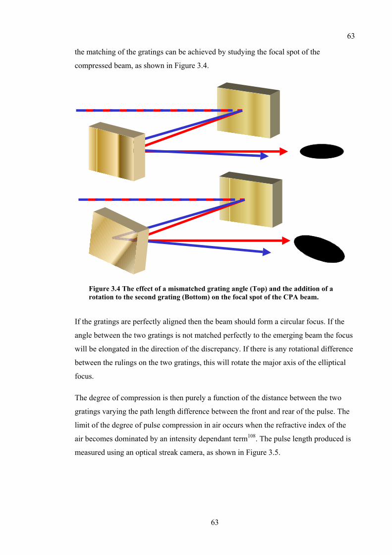
63
63
the matching of the gratings can be achieved by studying the focal spot of the
compressed beam, as shown in Figure 3.4.
Figure 3.4 The effect of a mismatched grating angle (Top) and the addition of a rotation to the second grating (Bottom) on the focal spot of the CPA beam.
If the gratings are perfectly aligned then the beam should form a circular focus. If the
angle between the two gratings is not matched perfectly to the emerging beam the focus
will be elongated in the direction of the discrepancy. If there is any rotational difference
between the rulings on the two gratings, this will rotate the major axis of the elliptical
focus.
The degree of compression is then purely a function of the distance between the two
gratings varying the path length difference between the front and rear of the pulse. The
limit of the degree of pulse compression in air occurs when the refractive index of the
air becomes dominated by an intensity dependant term108. The pulse length produced is
measured using an optical streak camera, as shown in Figure 3.5.

64
64
0
50
100
150
200
250
-100 -80 -60 -40 -20 0 20 40 60 80 100
Time (ps)
Inte
nsity
(a.u
.)
CPA probe pulse80ps Probe pulse
Figure 3.5 Probe beam pulse shapes for the first experiment (red) and the second and third experiments (blue)
3.4.3 Wavelength selection
The first requirement for selecting an appropriate wavelength to use as a probe for
propagation through the plasma is that the critical density for the wavelength selected is
much greater than the expected electron density in the plasma. This is in order to
minimise refractive effects and to allow simplifications of the treatment of the refractive
index to be valid (see section 3.2.1). As the plasma we are studying is of a relatively
low-density of 1018 cm-3, visible wavelength light at 527nm with a critical density of
4x1021 cm-3 satisfies these criteria. For probing higher densities, X-ray lasers have been
used for interferometric studies109.
The VULCAN beams used for the production of plasma are all at the fundamental
wavelength of the laser at 1054nm. As there will be a large amount of light scattered off
the target at this wavelength it is important that a different wavelength is used to probe
the plasma. The method employed is frequency doubling of the beam by use of a
Potassium-Dihydrogen-Phosphate (KDP) crystal. This process is another standard
technique employed on VULCAN for wavelength conversion, and is typically 50%
efficient.

65
65
When the beam is frequency doubled in the crystal, there is a small difference between
the incident and exiting direction of the beam. This has to be accounted for in any
alignment system.
The drawback of utilising frequency-doubled light is that this harmonic is also
generated by the laser plasma interaction. The possibility of Raman shifting110 the probe
to 622nm using an ethanol cell was investigated experimentally to overcome this
problem. Unfortunately, we were unable to produce a significant degree of conversion
through the Raman cell during our experimental set-up time. However, the level of
harmonic emission measured in the plasma is between two and three orders of
magnitude below the probe beam hence the Raman shift was not required.
3.4.4 Intensity selection
The intensity of the probe beam must be sufficient that the level of self-emission and
harmonic generation from the plasma at the probe wavelength is comparatively
insignificant. Working with high intensity lasers poses a significant problem when using
delicate optics. The optical components used to construct beamlines and diagnostics can
be damaged by the laser if it is sufficiently intense. Manufacturers publish guidelines on
the damage threshold of each component, normally in terms of the power of a
continuous beam or the energy of a standard 1ns pulse.
Unfortunately, the specifications of the probe beamlines utilised in our experiments are
far from the standard pulses used by optics manufacturers. The scaling of damage
threshold with pulse duration has been investigated at VULCAN111 for CPA pulse
lengths similar to the utilised probe designs. It was determined that for a 10 ps pulse the
damage threshold for a coated mirror would be 0.9 J/cm2, and for a 50ps pulse it would
be 1.5 J/cm2. This damage threshold is not an absolute value for damage to occur,
rather it is a value at which damage is significantly likely to occur. Intensities below the
threshold may still cause damage over time. In all three of the experiments performed
the background emission from the plasma is between two and three orders of magnitude
below the probe beam.
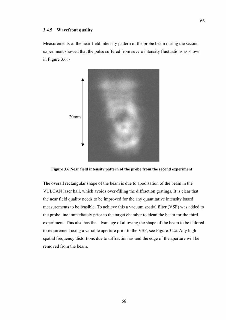
66
66
3.4.5 Wavefront quality
Measurements of the near-field intensity pattern of the probe beam during the second
experiment showed that the pulse suffered from severe intensity fluctuations as shown
in Figure 3.6: -
Figure 3.6 Near field intensity pattern of the probe from the second experiment
The overall rectangular shape of the beam is due to apodisation of the beam in the
VULCAN laser hall, which avoids over-filling the diffraction gratings. It is clear that
the near field quality needs to be improved for the any quantitative intensity based
measurements to be feasible. To achieve this a vacuum spatial filter (VSF) was added to
the probe line immediately prior to the target chamber to clean the beam for the third
experiment. This also has the advantage of allowing the shape of the beam to be tailored
to requirement using a variable aperture prior to the VSF, see Figure 3.2c. Any high
spatial frequency distortions due to diffraction around the edge of the aperture will be
removed from the beam.
20mm
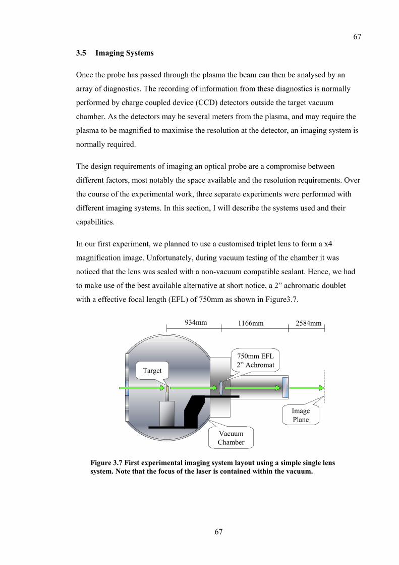
67
67
3.5 Imaging Systems
Once the probe has passed through the plasma the beam can then be analysed by an
array of diagnostics. The recording of information from these diagnostics is normally
performed by charge coupled device (CCD) detectors outside the target vacuum
chamber. As the detectors may be several meters from the plasma, and may require the
plasma to be magnified to maximise the resolution at the detector, an imaging system is
normally required.
The design requirements of imaging an optical probe are a compromise between
different factors, most notably the space available and the resolution requirements. Over
the course of the experimental work, three separate experiments were performed with
different imaging systems. In this section, I will describe the systems used and their
capabilities.
In our first experiment, we planned to use a customised triplet lens to form a x4
magnification image. Unfortunately, during vacuum testing of the chamber it was
noticed that the lens was sealed with a non-vacuum compatible sealant. Hence, we had
to make use of the best available alternative at short notice, a 2” achromatic doublet
with a effective focal length (EFL) of 750mm as shown in Figure3.7.
934mm 1166mm
Target
750mm EFL2” Achromat
VacuumChamber
ImagePlane
2584mm
Figure 3.7 First experimental imaging system layout using a simple single lens system. Note that the focus of the laser is contained within the vacuum.

68
68
For our second experiment a high-resolution image was required, but at a lower
magnification of x2.5. A customised f/2.5 spaced doublet lens pair was built based on a
design developed using the Zemax™ optics design package112 in conjunction with the
VULCAN laser staff, this is detailed in Figure 3.8:
284mm 1376mm
Target
108mm diameterf/2.5 doublet
VacuumChamber
ImagePlane
529mm
108mm diameteraspheric f/10
10.4mm
Figure 3.8 Second experimental imaging system using a more complex lens system. Two f/2.5 plano-convex lenses are used inside the chamber with a custom built spacer separating them by 10.4mm The image is then formed by a third lens outside the vacuum chamber.
In our third experiment, the diagnostics required an imaging system that utilised an
expanding beam to form the image, as opposed to the second experimental design
where the image is formed by a slowly converging beam. Diagnostics for this
experiment were to include a self-referencing interferometer. For this design various
catalogue single lens systems were evaluated using the OSLO™ optics package113. The
final design utilised a 3” 750mm EFL NPAC097 lens at x2.5 magnification as shown in
Figure 3.9.
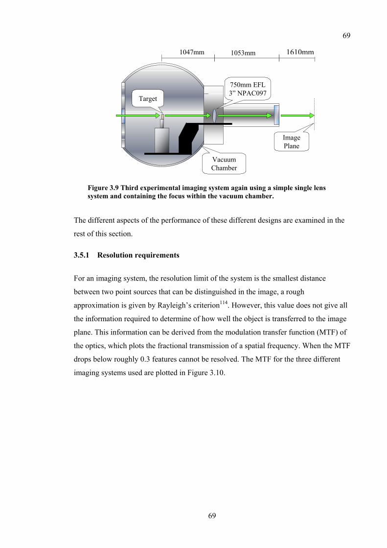
69
69
1047mm 1053mm
Target
750mm EFL3” NPAC097
VacuumChamber
ImagePlane
2599mm
Figure 3.9 Third experimental imaging system again using a simple single lens system and containing the focus within the vacuum chamber.
The different aspects of the performance of these different designs are examined in the
rest of this section.
3.5.1 Resolution requirements
For an imaging system, the resolution limit of the system is the smallest distance
between two point sources that can be distinguished in the image, a rough
approximation is given by Rayleigh’s criterion114. However, this value does not give all
the information required to determine of how well the object is transferred to the image
plane. This information can be derived from the modulation transfer function (MTF) of
the optics, which plots the fractional transmission of a spatial frequency. When the MTF
drops below roughly 0.3 features cannot be resolved. The MTF for the three different
imaging systems used are plotted in Figure 3.10.
1610mm
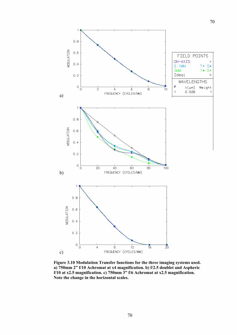
70
70
a)
b)
c)
Figure 3.10 Modulation Transfer functions for the three imaging systems used. a) 750mm 2” f/10 Achromat at x4 magnification. b) f/2.5 doublet and Aspheric f/10 at x2.5 magnification. c) 750mm 3” f/6 Achromat at x2.5 magnification. Note the change in the horizontal scales.
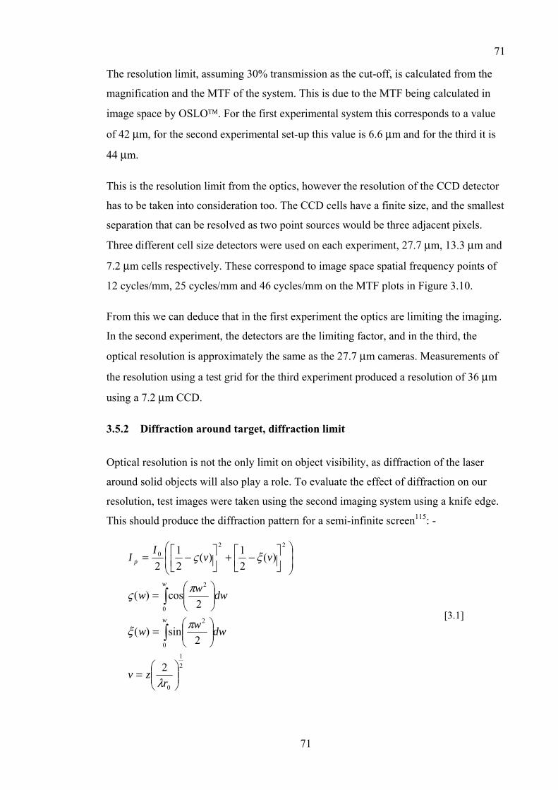
71
71
The resolution limit, assuming 30% transmission as the cut-off, is calculated from the
magnification and the MTF of the system. This is due to the MTF being calculated in
image space by OSLO™. For the first experimental system this corresponds to a value
of 42 µm, for the second experimental set-up this value is 6.6 µm and for the third it is
44 µm.
This is the resolution limit from the optics, however the resolution of the CCD detector
has to be taken into consideration too. The CCD cells have a finite size, and the smallest
separation that can be resolved as two point sources would be three adjacent pixels.
Three different cell size detectors were used on each experiment, 27.7 µm, 13.3 µm and
7.2 µm cells respectively. These correspond to image space spatial frequency points of
12 cycles/mm, 25 cycles/mm and 46 cycles/mm on the MTF plots in Figure 3.10.
From this we can deduce that in the first experiment the optics are limiting the imaging.
In the second experiment, the detectors are the limiting factor, and in the third, the
optical resolution is approximately the same as the 27.7 µm cameras. Measurements of
the resolution using a test grid for the third experiment produced a resolution of 36 µm
using a 7.2 µm CCD.
3.5.2 Diffraction around target, diffraction limit
Optical resolution is not the only limit on object visibility, as diffraction of the laser
around solid objects will also play a role. To evaluate the effect of diffraction on our
resolution, test images were taken using the second imaging system using a knife edge.
This should produce the diffraction pattern for a semi-infinite screen115: -
21
0
0
2
0
2
220
2
2sin)(
2cos)(
)(21)(
21
2
⎟⎟⎠
⎞⎜⎜⎝
⎛=
⎟⎟⎠
⎞⎜⎜⎝
⎛=
⎟⎟⎠
⎞⎜⎜⎝
⎛=
⎟⎟⎠
⎞⎜⎜⎝
⎛⎥⎦⎤
⎢⎣⎡ −+⎥⎦
⎤⎢⎣⎡ −=
∫
∫
rzv
dwww
dwww
vvI
I
w
w
p
λ
πξ
πς
ξς
[3.1]
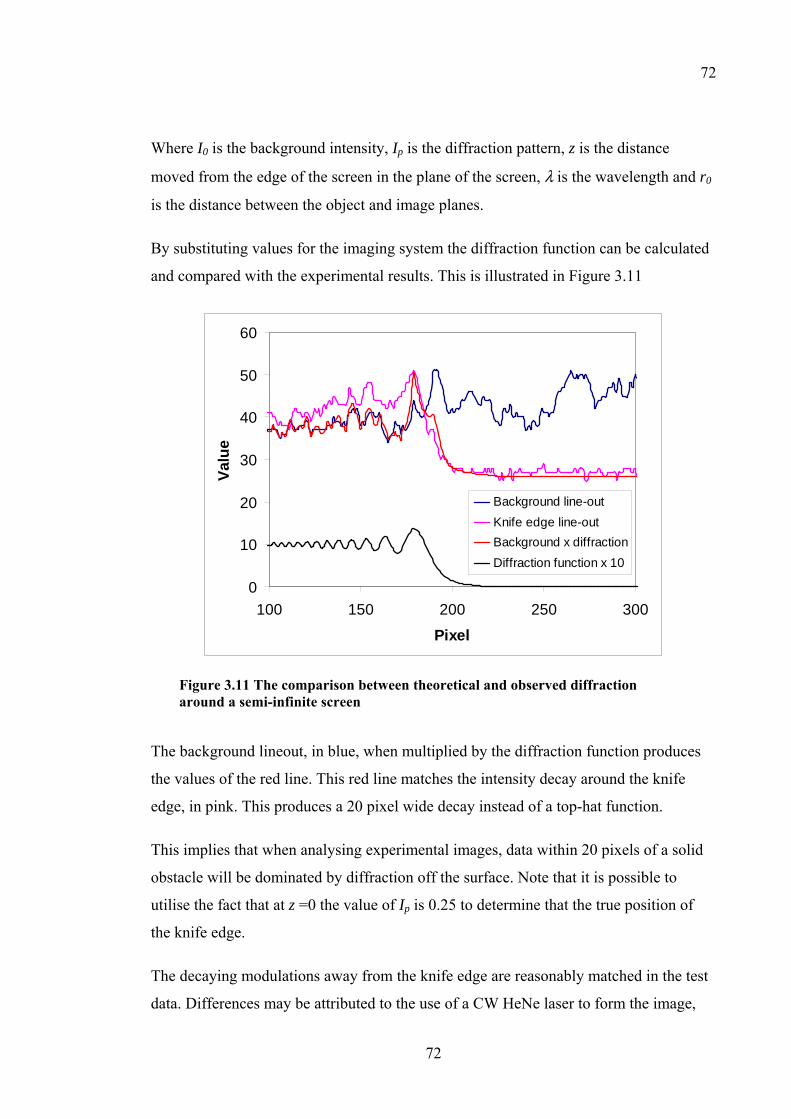
72
72
Where I0 is the background intensity, Ip is the diffraction pattern, z is the distance
moved from the edge of the screen in the plane of the screen, λ is the wavelength and r0
is the distance between the object and image planes.
By substituting values for the imaging system the diffraction function can be calculated
and compared with the experimental results. This is illustrated in Figure 3.11
0
10
20
30
40
50
60
100 150 200 250 300
Pixel
Valu
e
Background line-outKnife edge line-outBackground x diffractionDiffraction function x 10
Figure 3.11 The comparison between theoretical and observed diffraction around a semi-infinite screen
The background lineout, in blue, when multiplied by the diffraction function produces
the values of the red line. This red line matches the intensity decay around the knife
edge, in pink. This produces a 20 pixel wide decay instead of a top-hat function.
This implies that when analysing experimental images, data within 20 pixels of a solid
obstacle will be dominated by diffraction off the surface. Note that it is possible to
utilise the fact that at z =0 the value of Ip is 0.25 to determine that the true position of
the knife edge.
The decaying modulations away from the knife edge are reasonably matched in the test
data. Differences may be attributed to the use of a CW HeNe laser to form the image,
73
73
which produces slight time dependent intensity variations in the expanded beam.
Diffraction modulations in experimental data are distinguished by their monotonic
decay parallel to the surface that generated them.
3.5.3 Imaging for Interferometry
If any form of interferometric data is to be taken using the probe it is important that the
imaging system does not distort the wavefront of the beam. The method used to
evaluate this is the optical path difference (OPD). This is a function for each point on
the image plane, which describes the path length difference between all the possible
routes that could be taken by a ray to form the image relative to a reference ray. In
Figure 3.12, the OPD of each of the three imaging systems is plotted for three test
points. The reference ray used by OSLO™ to calculate the OPD is the central ray
through the system.
The OPD plots show that the first system benefits from having a high magnification,
helping to produce a roughly constant OPD over the field with a maximum difference of
0.027 wavelengths. The second and third imaging systems show more variation off axis,
with the second system becoming noticeably distorted at 3mm, the expected maximum
size of the plasma during the experimental timescale.
The maximum OPD of the second design would produce a 0.65 wavelength distortion,
enough to be easily measured by an interferometer. The third imaging system has a
maximum OPD of 0.009 wavelengths, which would require an interferometer with a
resolution of 1/100 of a fringe to resolve.
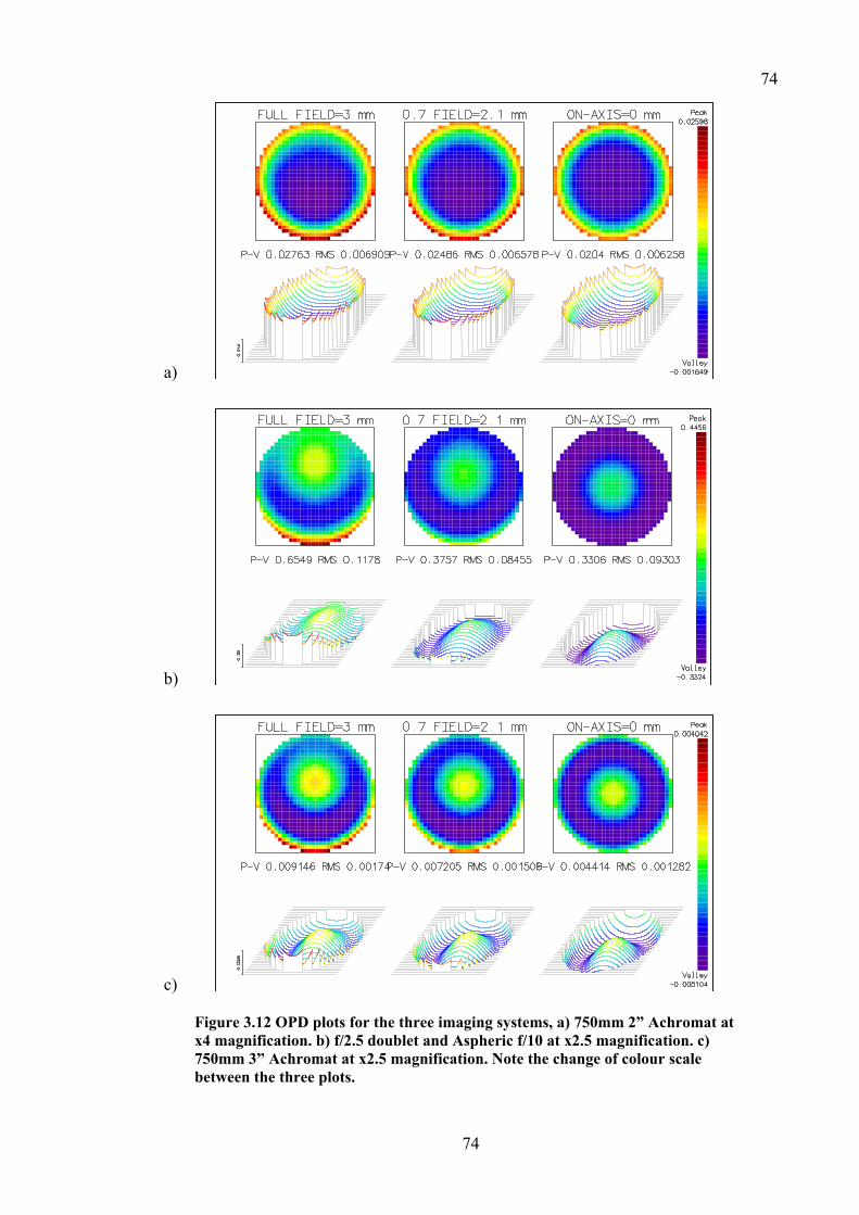
74
74
a)
b)
c)
Figure 3.12 OPD plots for the three imaging systems, a) 750mm 2” Achromat at x4 magnification. b) f/2.5 doublet and Aspheric f/10 at x2.5 magnification. c) 750mm 3” Achromat at x2.5 magnification. Note the change of colour scale between the three plots.
75
75
3.5.4 Limitations due to refraction
For a measurement using refraction, for example Schlieren imaging, that has occurred in
the plasma, the upper limit of the measurement is governed by the collecting angle of
the imaging system. In all three imaging systems, the limiting aperture in this case is the
first collecting lens. Hence for the first experiment the collection angle is 1.55 degrees,
for the second experiment it is 20.8 degrees and for the third experiment it is 2.08
degrees.
3.6 Conclusions
In this chapter, I have shown propagation of light through a plasma can be treated using
the geometric optics approach and a knowledge of the refractive index of a plasma. This
has been used to develop a beamline for optically probing a plasma suitable for different
experimental requirements. An evaluation of the performance of the implemented
designs has been presented in terms of the resolution of the imaging, the distortion to
the wavefront, the effects of diffraction around the target holder and the limitations on
refraction based measurements.
In our first experiment, we find that the resolution of the system implemented is limited
by the duration of the pulse length. In our second design the resolution is limited by the
diagnostic recording media and not the optical system through the use of a CPA pulse
and custom designed optics. However, this design is not suitable for all types of
diagnostic. The further addition of a VSF to improve the nearfield and a single lens
system was used for the final experiment to allow interferometry and polarimetry
measurements to be made with a resolution comparable with the recording media.
76
76
4 Chapter 4 - Optical probe diagnostics
4.1 Introduction
Following the description of the probe beam and the imaging system in the previous
chapter, the diagnostics used to study how the plasma modifies the probe beam are now
described. These diagnostics include shadowgraphy to produce an ‘image’ of the
plasma, interferometery used to extract quantitative ne measurements, Schlieren imaging
used to extract qualitative measurements of ∇ne, and polarimetry to extract B. The
theory supporting these measurements, the designs, and the techniques used to analyse
the data are described.
4.2 Interferometry
4.2.1 Theory
The basic principle of an interferometer is the measurement of phase differences
between two coherent beams of light. If two beams interfere with each other the sum of
the electric field vectors is observed. For two beams with a phase difference θ which
can be described as
))(exp()exp(
θωω
+titi
2
1
EE
[4.1]
Then on interference the electric fields add to give
)exp())exp(( tii ωθ21t EEE += [4.2]
Which when measured on an intensity based detector leads to a cos(θ) distribution.
When a probe beam propagates for a length l, through medium of refractive index n
(where n≠1), the phase of the beam will be retarded by an amount φ where
∫= ldc
n ωφ [4.3]

77
77
If the probe beam then interferes with a reference beam that has just propagated through
an equal distance in vacuum (where n=1) then the phase difference between the two
beams will be
∫ −= ldc
n ωθ )1( [4.4]
This result is useful as the refractive index of the plasma to a first order approximation
is a function of the electron density of the plasma (see derivation of [3.13])
c
e
nnn −= 1 [4.5]
Which for a value of the electron density much smaller than the critical density can be
approximated to
c
e
nnn
21−= [4.6]
If this result is substituted into the phase difference [4.4] we can see that
∫∫ == ll dncn
dcn
ne
cc
e
22ωωθ [4.7]
Implying that the phase shift is proportional to the path integrated electron density.
Hence by measuring the interference pattern it is possible to evaluate the electron
density of the plasma, ne.
A simple assumption for estimating the interference pattern produced by the plasma is
to assume the path of the ray will be a straight line. This should be approximately valid
for ne << nc, the condition already assumed in this derivation.
For this case the phase difference can be considered as an addition to a background
interference pattern on the interferometer with a given fringe spacing. For a 1mm
diameter cylindrical plasma modelled by Medusa propagating the probe perpendicular
to the cylinder’s axis, the resulting fringe pattern for a x3.6 magnification imaging
interferometer recorded on a 7µm cell CCD camera with a background fringe spacing of
around 60µm should resemble Figure 4.1.
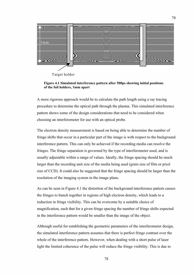
78
78
Target holder
1mm
Figure 4.1 Simulated interference pattern after 500ps showing initial positions of the foil holders, 1mm apart
A more rigorous approach would be to calculate the path length using a ray tracing
procedure to determine the optical path through the plasma. This simulated interference
pattern shows some of the design considerations that need to be considered when
choosing an interferometer for use with an optical probe.
The electron density measurement is based on being able to determine the number of
fringe shifts that occur in a particular part of the image is with respect to the background
interference pattern. This can only be achieved if the recording media can resolve the
fringes. The fringe separation is governed by the type of interferometer used, and is
usually adjustable within a range of values. Ideally, the fringe spacing should be much
larger than the recording unit size of the media being used (grain size of film or pixel
size of CCD). It could also be suggested that the fringe spacing should be larger than the
resolution of the imaging system in the image plane.
As can be seen in Figure 4.1 the distortion of the background interference pattern causes
the fringes to bunch together in regions of high electron density, which leads to a
reduction in fringe visibility. This can be overcome by a suitable choice of
magnification, such that for a given fringe spacing the number of fringe shifts expected
in the interference pattern would be smaller than the image of the object.
Although useful for establishing the geometric parameters of the interferometer design,
the simulated interference pattern assumes that there is perfect fringe contrast over the
whole of the interference pattern. However, when dealing with a short pulse of laser
light the limited coherence of the pulse will reduce the fringe visibility. This is due to

79
79
the polychromatic nature of the source, where if an interference pattern is formed for
one particular wavelength the other wavelength components that form the beam will
gradually slip out of phase and interfere destructively the further away from zero path
difference you go. Hence, the further away from zero path difference a point on the
image lies, the worse the fringe contrast becomes, and in effect limits the number of
fringes that would be visible in the interference pattern.
The coherence length of the probe is governed predominantly by the bandwidth ∆λ of
the pulse for a short pulse probe. The coherence length for a beam of wavelength λ can
be considered to be116: -
λλ∆
≈∆2
tc [4.8]
The values for the system used in our experiments are λ = 527nm and ∆λ = 6nm, this
gives a coherence length of 46µm or a total of 87 visible fringes.
4.2.2 Interferometer Designs
There are several different types of interferometer design that can be used for
measurements in plasmas117. As noted above, the coherence length of the probe is likely
to be very short which requires that the interferometer introduces a zero path length
difference between the reference and data wavefronts. Hence, a form of interferometer
has to be used that is self referencing, to avoid coherence length complications. In our
experiments, we have used Vertical shearing and modified Normarski interferometer
designs. The modified Normarski interferometer is based on the use of a polarisation
splitting prism, in our case a Wollaston prism118. The prism is used to provide a
reference from a section of the beam that is not distorted by the object being studied as
shown in Figure 4.2 below. The main advantage of this design is the simplicity of the
set-up, as there are no delicate alignment issues and the plane in the middle of the
overlapping beam will always have zero path difference.
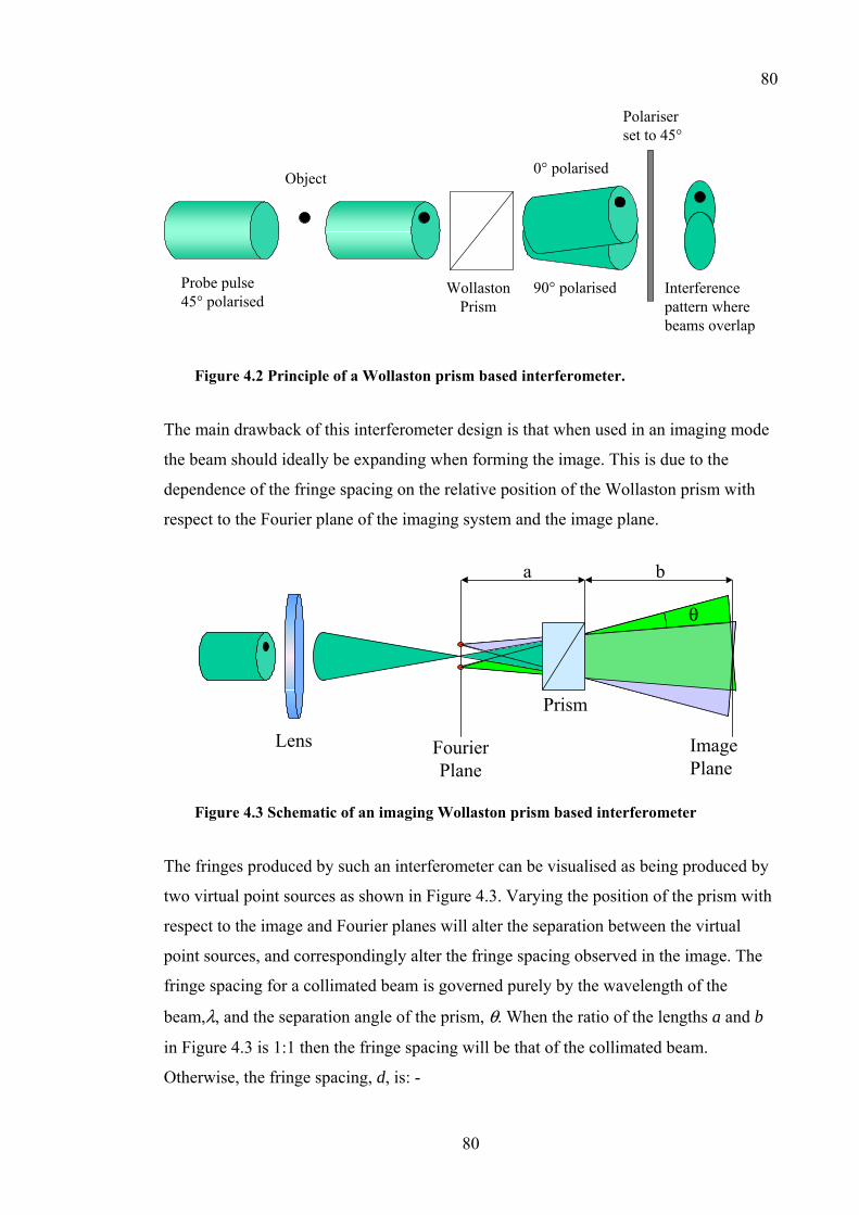
80
80
Probe pulse45° polarised
Object
WollastonPrism
Polariserset to 45°
0° polarised
90° polarised Interferencepattern wherebeams overlap
Figure 4.2 Principle of a Wollaston prism based interferometer.
The main drawback of this interferometer design is that when used in an imaging mode
the beam should ideally be expanding when forming the image. This is due to the
dependence of the fringe spacing on the relative position of the Wollaston prism with
respect to the Fourier plane of the imaging system and the image plane.
FourierPlane
ImagePlane
Prism
a b
Lens
θ
Figure 4.3 Schematic of an imaging Wollaston prism based interferometer
The fringes produced by such an interferometer can be visualised as being produced by
two virtual point sources as shown in Figure 4.3. Varying the position of the prism with
respect to the image and Fourier planes will alter the separation between the virtual
point sources, and correspondingly alter the fringe spacing observed in the image. The
fringe spacing for a collimated beam is governed purely by the wavelength of the
beam,λ, and the separation angle of the prism, θ. When the ratio of the lengths a and b
in Figure 4.3 is 1:1 then the fringe spacing will be that of the collimated beam.
Otherwise, the fringe spacing, d, is: -
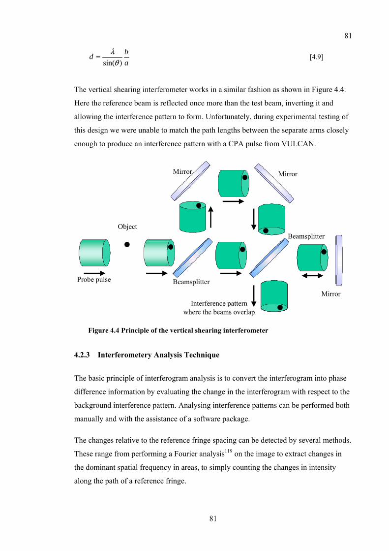
81
81
abd
)sin(θλ= [4.9]
The vertical shearing interferometer works in a similar fashion as shown in Figure 4.4.
Here the reference beam is reflected once more than the test beam, inverting it and
allowing the interference pattern to form. Unfortunately, during experimental testing of
this design we were unable to match the path lengths between the separate arms closely
enough to produce an interference pattern with a CPA pulse from VULCAN.
Probe pulse
Object
Interference patternwhere the beams overlap
Beamsplitter
Mirror
Beamsplitter
Mirror
Mirror
Figure 4.4 Principle of the vertical shearing interferometer
4.2.3 Interferometery Analysis Technique
The basic principle of interferogram analysis is to convert the interferogram into phase
difference information by evaluating the change in the interferogram with respect to the
background interference pattern. Analysing interference patterns can be performed both
manually and with the assistance of a software package.
The changes relative to the reference fringe spacing can be detected by several methods.
These range from performing a Fourier analysis119 on the image to extract changes in
the dominant spatial frequency in areas, to simply counting the changes in intensity
along the path of a reference fringe.
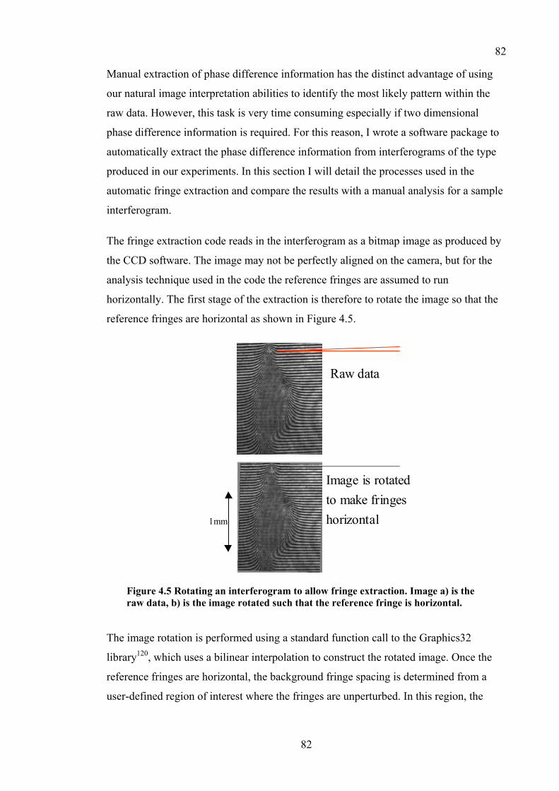
82
82
Manual extraction of phase difference information has the distinct advantage of using
our natural image interpretation abilities to identify the most likely pattern within the
raw data. However, this task is very time consuming especially if two dimensional
phase difference information is required. For this reason, I wrote a software package to
automatically extract the phase difference information from interferograms of the type
produced in our experiments. In this section I will detail the processes used in the
automatic fringe extraction and compare the results with a manual analysis for a sample
interferogram.
The fringe extraction code reads in the interferogram as a bitmap image as produced by
the CCD software. The image may not be perfectly aligned on the camera, but for the
analysis technique used in the code the reference fringes are assumed to run
horizontally. The first stage of the extraction is therefore to rotate the image so that the
reference fringes are horizontal as shown in Figure 4.5.
Raw data
Image is rotatedto make fringeshorizontal1mm
Figure 4.5 Rotating an interferogram to allow fringe extraction. Image a) is the raw data, b) is the image rotated such that the reference fringe is horizontal.
The image rotation is performed using a standard function call to the Graphics32
library120, which uses a bilinear interpolation to construct the rotated image. Once the
reference fringes are horizontal, the background fringe spacing is determined from a
user-defined region of interest where the fringes are unperturbed. In this region, the
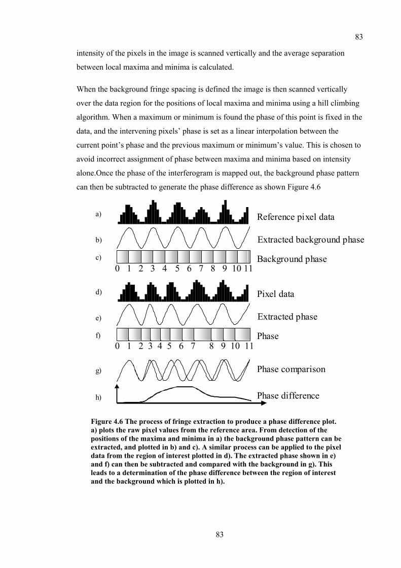
83
83
intensity of the pixels in the image is scanned vertically and the average separation
between local maxima and minima is calculated.
When the background fringe spacing is defined the image is then scanned vertically
over the data region for the positions of local maxima and minima using a hill climbing
algorithm. When a maximum or minimum is found the phase of this point is fixed in the
data, and the intervening pixels’ phase is set as a linear interpolation between the
current point’s phase and the previous maximum or minimum’s value. This is chosen to
avoid incorrect assignment of phase between maxima and minima based on intensity
alone.Once the phase of the interferogram is mapped out, the background phase pattern
can then be subtracted to generate the phase difference as shown Figure 4.6
0 1 2 3 4 5 6 7 8 9 10 11
Reference pixel data
Extracted background phase
Background phase
0 1 2 3 4 5 6 7 8 9 10 11
Pixel data
Extracted phase
Phase
Phase comparison
Phase difference
a)
b)
c)
d)
e)
f)
g)
h)
Figure 4.6 The process of fringe extraction to produce a phase difference plot. a) plots the raw pixel values from the reference area. From detection of the positions of the maxima and minima in a) the background phase pattern can be extracted, and plotted in b) and c). A similar process can be applied to the pixel data from the region of interest plotted in d). The extracted phase shown in e) and f) can then be subtracted and compared with the background in g). This leads to a determination of the phase difference between the region of interest and the background which is plotted in h).
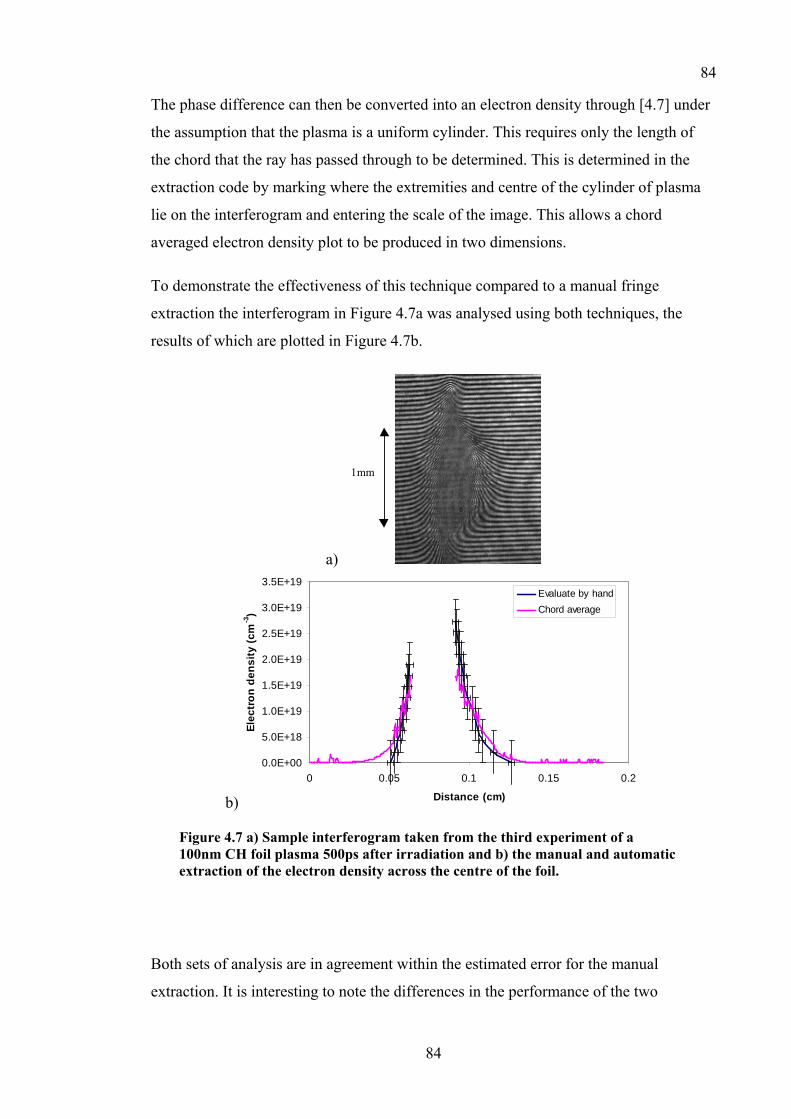
84
84
The phase difference can then be converted into an electron density through [4.7] under
the assumption that the plasma is a uniform cylinder. This requires only the length of
the chord that the ray has passed through to be determined. This is determined in the
extraction code by marking where the extremities and centre of the cylinder of plasma
lie on the interferogram and entering the scale of the image. This allows a chord
averaged electron density plot to be produced in two dimensions.
To demonstrate the effectiveness of this technique compared to a manual fringe
extraction the interferogram in Figure 4.7a was analysed using both techniques, the
results of which are plotted in Figure 4.7b.
a)
1mm
b)
0.0E+00
5.0E+18
1.0E+19
1.5E+19
2.0E+19
2.5E+19
3.0E+19
3.5E+19
0 0.05 0.1 0.15 0.2
Distance (cm)
Elec
tron
den
sity
(cm
-3)
Evaluate by handChord average
Figure 4.7 a) Sample interferogram taken from the third experiment of a 100nm CH foil plasma 500ps after irradiation and b) the manual and automatic extraction of the electron density across the centre of the foil.
Both sets of analysis are in agreement within the estimated error for the manual
extraction. It is interesting to note the differences in the performance of the two
85
85
techniques. In the higher density regions the manual extraction produces results that are
more credible as the human eye is able to discern rapid fringe shifts far more accurately
than the analysis code. On the other hand, at low densities the automatic analysis is able
to detect very small shifts in the fringe positions better than the manual extraction. This
is significant as the data we are interested in extracting from the interferograms is in this
low-density expansion region.
4.2.4 Abel inversion
The chord averaged electron density profiles described in the previous section rely on
the assumption that the plasma has a uniform radial density profile. However, this may
not always be the case. If the electron density profile contains a symmetric radial
component this can be extracted from the phase difference data using the technique of
Abel inversion. The Abel transformation converts a chordal integral, such as the phase
difference measurement, into a radial value, the electron density, as described by
Hutchinson121.
As there are often greater than 200 separate measurements of the chordal integral from
the data collected, it was possible to perform Abel inversion on the phase difference
data without having to fit a curve to the data. The test of the Abel inversion method is to
extract an electron density profile where there is known to be a cylindrically symmetric
feature in the plasma. This was achieved by using 100nm thick CH foil targets with a
200µm diameter aluminium dot coated onto its surface. The emission from this plasma
in the direction viewed by the probe beam polarimetry diagnostic in the absence of a
probe pulse and is shown in Figure 4.8.

86
86
1mm
Figure 4.8 Broadband emission from a 200µm diameter Al dot coated onto a 100nm thick CH foil irradiated by two 40J 80ps beams from VULCAN.
The extent of the aluminium portion of the plasma can clearly be seen in the emission as
a tapering spike. Analysis of the interferometery data for this type of target
demonstrates the ability of the Abel inversion technique to extract radial detail from the
data as shown in Figure 4.9
.
1mm
1019cm-3 1018cm-3
b)
1019cm-3 1018cm-3
Figure 4.9 Contour plots of the a) chord averaged data and b) the Abel inverted data. The images plot electron density contours every decade with the peak contour in both images occurring at 1019 cm-3

87
87
Figure 4.9b shows a central tapering density spike in the Abel inverted data of the type
observed in the broadband emission of Figure 4.8, which is not present in the chord
averaged data. Closer examination shows the diameter of this central feature as close to
the initial foil position to be 186 +/- 5µm, very close to the nominal 200µm diameter of
the coated dot.
4.3 Shadowgraphy and Schlieren Imaging
4.3.1 Theory
When light from a probe beam exits inhomogeneous plasma it can be seen from section
3.2.2, that the exit angle of the ray is different to the entrance angle. The angular
deviation is proportional to the integrated gradient of the refractive index of the plasma
over the ray’s path. As already shown in section 3.2.1, the refractive index, to a first
approximation, is a function of the electron density of the plasma. This implies that the
degree of deflection is a function of the electron density gradient. This deflection can be
visualised by dark field Schlieren imaging.
Schlieren imaging is a standard technique for visualising refractive index fluctuations
that would normally be transparent in an image122. The dark field schlieren image is
produced by focussing the probe beam onto a beam stop and imaging the rays that have
been deflected and pass around this beam stop, as shown Figure 4.10. Many varieties of
beam stops can be used, with the most common for light field schlieren imaging being
the knife-edge. This type of stop allows all of the light from one half of the imaged
object to form a background image, on top of which an additional component due to the
deviated rays is added. Dark field imaging uses a circular beam stop so that only the
deviated rays form the resultant image. The degree of deflection that is required for the
ray to arrive at the image plane is equal to the angle subtended by the stop at the focal
length of the lens being used. Hence, the sensitivity of the image is governed by the size
of the stop. The upper limit on the amount of refraction that can be detected is the
limiting aperture of the imaging system, as described in section 3.5.4.
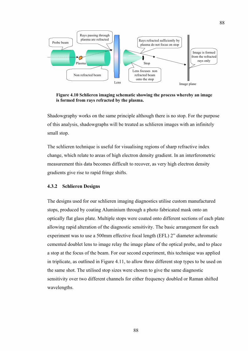
88
88
Plasma
Lens
Stop
Rays refracted sufficiently by plasma do not focus on stop
Image plane
Lens focuses nonrefracted beamonto the stop
Probe beam
Rays passing throughplasma are refracted
Image is formedfrom the refracted
rays only
Non refracted beam
Figure 4.10 Schlieren imaging schematic showing the process whereby an image is formed from rays refracted by the plasma.
Shadowgraphy works on the same principle although there is no stop. For the purpose
of this analysis, shadowgraphs will be treated as schlieren images with an infinitely
small stop.
The schlieren technique is useful for visualising regions of sharp refractive index
change, which relate to areas of high electron density gradient. In an interferometric
measurement this data becomes difficult to recover, as very high electron density
gradients give rise to rapid fringe shifts.
4.3.2 Schlieren Designs
The designs used for our schlieren imaging diagnostics utilise custom manufactured
stops, produced by coating Aluminium through a photo fabricated mask onto an
optically flat glass plate. Multiple stops were coated onto different sections of each plate
allowing rapid alteration of the diagnostic sensitivity. The basic arrangement for each
experiment was to use a 500mm effective focal length (EFL) 2” diameter achromatic
cemented doublet lens to image relay the image plane of the optical probe, and to place
a stop at the focus of the beam. For our second experiment, this technique was applied
in triplicate, as outlined in Figure 4.11, to allow three different stop types to be used on
the same shot. The utilised stop sizes were chosen to give the same diagnostic
sensitivity over two different channels for either frequency doubled or Raman shifted
wavelengths.

89
89
1000mm
500mm
1000mm
500mm
500mm
20%
80% 50%
50%
500mm EFL2” Achromatic Lens
ø1.1mm
ø2.1mm
ø1.6mm
HR @527nm mirror
Beam splitter
Image capture PC
Image plane
Figure 4.11 Schlieren imaging arrangement for second experiment
4.3.3 Ray tracing analysis
When interpreting schlieren images it is not possible to directly infer from an image the
exact magnitude of electron density gradient present in the plasma. It is possible to
deduce the approximate sensitivity of the schlieren imaging system by assuming a
known path length through the plasma and a constant density gradient, although this
will only give an approximate cut-off value. Forming multiple simultaneous images
with different size stops can enable a rough contour map of electron density gradient to
be produced. It is possible to make accurate positional measurements of features in the
images, which can be compared to the scale length of features present in the plasma.
However, a more complete form of analysis would be to form simulated schlieren
images123,124 that can be compared to the experimental data.
If there was an analytical solution to the ray path of a photon through the plasma then a
simulated image could be directly calculated. Simulated schlieren images can also be
formed through iterative ray tracing123 through an assumed plasma profile. Assuming
the deflection of the light passing through the plasma is sufficiently small, then the path
of the ray can be approximated as a straight-line124. For the plasma profile provided by
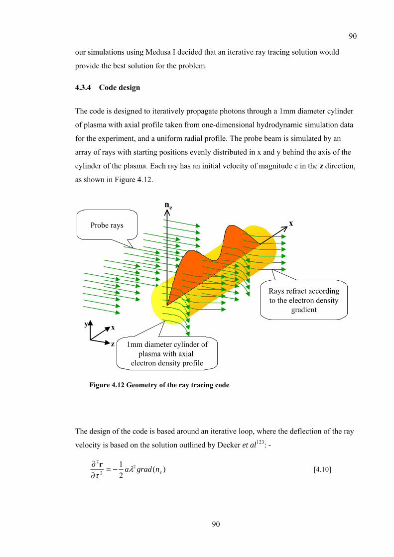
90
90
our simulations using Medusa I decided that an iterative ray tracing solution would
provide the best solution for the problem.
4.3.4 Code design
The code is designed to iteratively propagate photons through a 1mm diameter cylinder
of plasma with axial profile taken from one-dimensional hydrodynamic simulation data
for the experiment, and a uniform radial profile. The probe beam is simulated by an
array of rays with starting positions evenly distributed in x and y behind the axis of the
cylinder of the plasma. Each ray has an initial velocity of magnitude c in the z direction,
as shown in Figure 4.12.
y x
z
ne
xProbe rays
Rays refract accordingto the electron density
gradient
1mm diameter cylinder ofplasma with axial
electron density profile
Figure 4.12 Geometry of the ray tracing code
The design of the code is based around an iterative loop, where the deflection of the ray
velocity is based on the solution outlined by Decker et al123: -
)(21 2
2
2
engradaλτ
−=∂∂ r
[4.10]
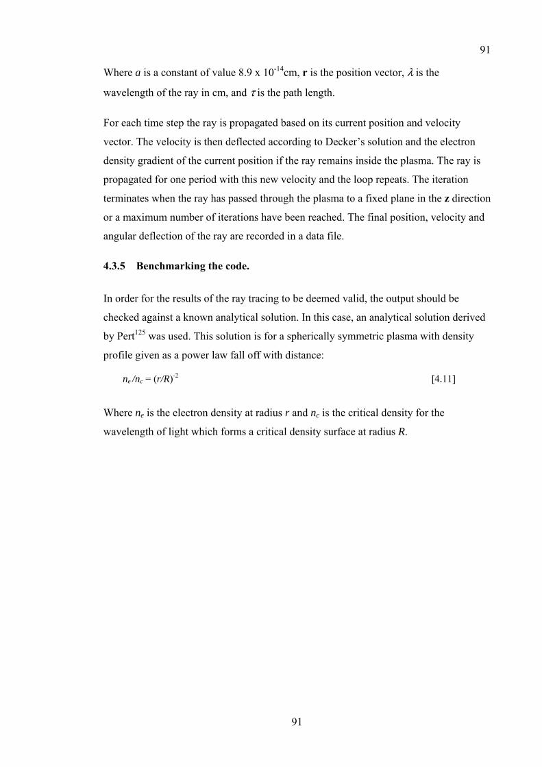
91
91
Where a is a constant of value 8.9 x 10⁻¹⁴cm, r is the position vector, λ is the
wavelength of the ray in cm, and τ is the path length.
For each time step the ray is propagated based on its current position and velocity
vector. The velocity is then deflected according to Decker’s solution and the electron
density gradient of the current position if the ray remains inside the plasma. The ray is
propagated for one period with this new velocity and the loop repeats. The iteration
terminates when the ray has passed through the plasma to a fixed plane in the z direction
or a maximum number of iterations have been reached. The final position, velocity and
angular deflection of the ray are recorded in a data file.
4.3.5 Benchmarking the code.
In order for the results of the ray tracing to be deemed valid, the output should be
checked against a known analytical solution. In this case, an analytical solution derived
by Pert125 was used. This solution is for a spherically symmetric plasma with density
profile given as a power law fall off with distance:
ne /nc = (r/R)-2 [4.11]
Where ne is the electron density at radius r and nc is the critical density for the
wavelength of light which forms a critical density surface at radius R.
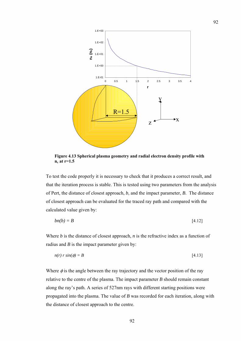
92
92
z x
y
1.E-01
1.E+00
1.E+01
1.E+02
1.E+03
0 0.5 1 1.5 2 2.5 3 3.5 4
rne
(nc)
R=1.5
Figure 4.13 Spherical plasma geometry and radial electron density profile with nc at r=1.5
To test the code properly it is necessary to check that it produces a correct result, and
that the iteration process is stable. This is tested using two parameters from the analysis
of Pert, the distance of closest approach, b, and the impact parameter, B. The distance
of closest approach can be evaluated for the traced ray path and compared with the
calculated value given by:
bn(b) = B [4.12]
Where b is the distance of closest approach, n is the refractive index as a function of
radius and B is the impact parameter given by:
n(r) r sin(φ) = B [4.13]
Where φ is the angle between the ray trajectory and the vector position of the ray
relative to the centre of the plasma. The impact parameter B should remain constant
along the ray’s path. A series of 527nm rays with different starting positions were
propagated into the plasma. The value of B was recorded for each iteration, along with
the distance of closest approach to the centre.

93
93
1.0E-08
1.0E-07
1.0E-06
1.0E-05
0.0E+00 1.0E-05 2.0E-05 3.0E-05 4.0E-05 5.0E-05 6.0E-05 7.0E-05
Distance of closest approach(m)
Erro
r (m
)
Figure 4.14 Values of the calculated minimum radius compared with simulation results, using the solution of Decker et al, for a critical density surface at 1.0 x 10⁻⁵m
The initial positions of the rays were selected to give a large variation in deflection
angle, ranging from complete reflection at the critical density surface for a normally
incident ray through to a deflection of 10-2 radians for the furthest ray used.
When evaluating the error in the simulation there are two processes at work. Firstly,
during each iteration the velocity of the ray is normalised to the local speed of light and
propagated for a fixed time, and can introduce inaccuracy for large changes in the local
speed of light over one iteration. Secondly, the calculations of the deflection, according
to the iterative solution may be in error. The differences between these two processes
can be seen in the special case of a normal incident ray. In this case, the magnitude of
the error is purely a reflection on the normalisation process. For a normally incident ray,
any error in the degree of deflection will be masked by the normalisation of the velocity
stopping the ray at the critical density surface. For a non-normally incident ray, any
error in the deflection calculation would be expected to fall off in line with the
integrated magnitude of the electron density gradient traversed by the ray. This can be
evaluated for the case of a ray with closest approach at an infinite distance from the
plasma centre, which should experience no error in propagation due to the deflection
calculation. For rays in between these two extremes, the error would be expected to be
approximately a 1/r2 profile; i.e. the error should decrease by an order of magnitude for
a threefold increase in distance of closest approach for a simulation purely limited by
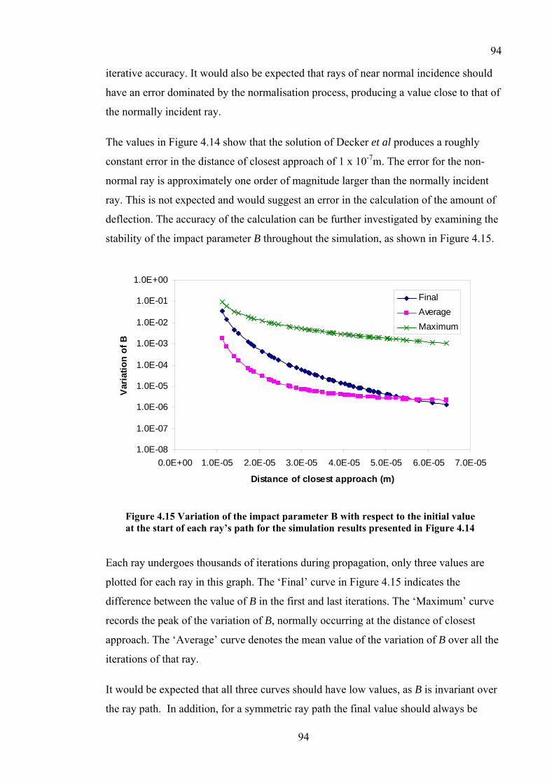
94
94
iterative accuracy. It would also be expected that rays of near normal incidence should
have an error dominated by the normalisation process, producing a value close to that of
the normally incident ray.
The values in Figure 4.14 show that the solution of Decker et al produces a roughly
constant error in the distance of closest approach of 1 x 10⁻⁷m. The error for the non-
normal ray is approximately one order of magnitude larger than the normally incident
ray. This is not expected and would suggest an error in the calculation of the amount of
deflection. The accuracy of the calculation can be further investigated by examining the
stability of the impact parameter B throughout the simulation, as shown in Figure 4.15.
1.0E-08
1.0E-07
1.0E-06
1.0E-05
1.0E-04
1.0E-03
1.0E-02
1.0E-01
1.0E+00
0.0E+00 1.0E-05 2.0E-05 3.0E-05 4.0E-05 5.0E-05 6.0E-05 7.0E-05
Distance of closest approach (m)
Var
iatio
n of
B
FinalAverageMaximum
Figure 4.15 Variation of the impact parameter B with respect to the initial value at the start of each ray’s path for the simulation results presented in Figure 4.14
Each ray undergoes thousands of iterations during propagation, only three values are
plotted for each ray in this graph. The ‘Final’ curve in Figure 4.15 indicates the
difference between the value of B in the first and last iterations. The ‘Maximum’ curve
records the peak of the variation of B, normally occurring at the distance of closest
approach. The ‘Average’ curve denotes the mean value of the variation of B over all the
iterations of that ray.
It would be expected that all three curves should have low values, as B is invariant over
the ray path. In addition, for a symmetric ray path the final value should always be
95
95
identical to the initial value, with a certain tolerance for numerical rounding. For
example, given a ray path with 10,000 iterations it would only require a factor of 10-6
numerical error on each iteration to produce a 1% variation in the final value. However,
there will be exceptions due to the iterative nature of the propagation. When the ray is
close to the plasma centre there is a greater uncertainty in determining the angle
between the position vector and the velocity vector when calculating the value of B . As
both vectors are normalised by their magnitude, for small radii positions, the length of
the propagation during the iteration will influence the calculation.
It would be expected that the ‘Average’ curve in Figure 4.15 should follow the same
behaviour as the ‘Final’ curve, if the iteration process is stable and accurate with only a
small number of anomalous values close to the turning point. The ‘Average’ curve
should also be lower than the ‘Final’ curve as the amount of variation is expected to
compound itself with every iteration, if the solution is limited only by numerical
accuracy.
However, Figure 4.15 shows that for Decker’s solution the ‘Average’ curve follows the
behaviour of the ‘Maximum’ curve, indicating that a significant amount of the iterations
differ from the expected behaviour indicated by the ‘Final’ curve. In addition, the
‘Average’ curve is larger than the ‘Final’ curve for distances of closest approach greater
than 5.5 x 10⁻⁵m. This suggests that the solution proposed by Decker et al123 is not
correct.
In the treatment derived by Decker et al a constant of 8.9x10⁻¹⁴cm is multiplied by the
square of the wavelength, with no explanation of the source of this constant. The
derivation of the full expression can be derived from Pert’s analysis125. Here we treat
the geometric optics problem as a single particle motion problem where the ratio of the
particles potential energy, V, of the particle to its total energy, E, is given by:
c
e
nn
EV = [4.14]
We can write the change in the particle velocity, v, caused by a variation in electron
density ne over an fixed distance ∆l as:

96
96
llv
∆
⎟⎟⎠
⎞⎜⎜⎝
⎛−−⎟⎟
⎠
⎞⎜⎜⎝
⎛ ∆+−
=∆∆
21
21
11c
e
c
ee
nn
cn
nnc
[4.15]
Where c is the speed of light. This can be approximated for small scale length variations
in the electron density, using the geometric optics assumption, to:
llv
∆
⎟⎟⎠
⎞⎜⎜⎝
⎛ ∆
≈∆∆
2c
e
nn
c [4.16]
By converting this velocity gradient into an acceleration we get:
⎟⎠
⎞⎜⎝
⎛∆
∆−=
∆∆
lv e
c
nnnc
t 2
2
[4.17]
As the wavelength dependency of Decker’s solution is included within the calculation
of the critical density, this solution could be re-written in the same format as [4.10].
This would produce a solution with a constant of 8.1705 x10⁻¹⁴cm, rather than 8.9 x
10-14cm. Modifying the ray tracing code to use the solution given in [4.17] produces the
results shown in Figure 4.16: -
1.0E-10
1.0E-09
1.0E-08
1.0E-07
0.0E+00 1.0E-05 2.0E-05 3.0E-05 4.0E-05 5.0E-05 6.0E-05 7.0E-05
Distance of closest approach(m)
Erro
r (m
)
Figure 4.16 Results of the modified ray tracing solution using identical input parameters for comparison with Figure 4.14
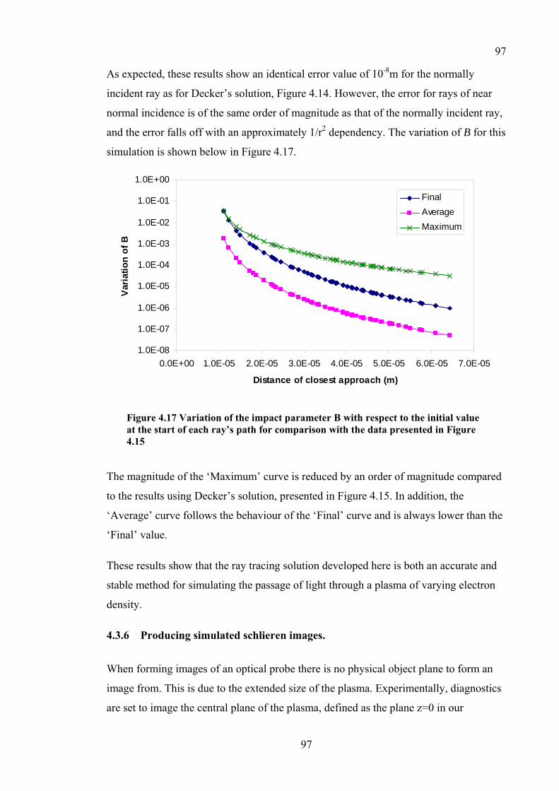
97
97
As expected, these results show an identical error value of 10-8m for the normally
incident ray as for Decker’s solution, Figure 4.14. However, the error for rays of near
normal incidence is of the same order of magnitude as that of the normally incident ray,
and the error falls off with an approximately 1/r2 dependency. The variation of B for this
simulation is shown below in Figure 4.17.
1.0E-08
1.0E-07
1.0E-06
1.0E-05
1.0E-04
1.0E-03
1.0E-02
1.0E-01
1.0E+00
0.0E+00 1.0E-05 2.0E-05 3.0E-05 4.0E-05 5.0E-05 6.0E-05 7.0E-05
Distance of closest approach (m)
Var
iatio
n of
B
FinalAverageMaximum
Figure 4.17 Variation of the impact parameter B with respect to the initial value at the start of each ray’s path for comparison with the data presented in Figure 4.15
The magnitude of the ‘Maximum’ curve is reduced by an order of magnitude compared
to the results using Decker’s solution, presented in Figure 4.15. In addition, the
‘Average’ curve follows the behaviour of the ‘Final’ curve and is always lower than the
‘Final’ value.
These results show that the ray tracing solution developed here is both an accurate and
stable method for simulating the passage of light through a plasma of varying electron
density.
4.3.6 Producing simulated schlieren images.
When forming images of an optical probe there is no physical object plane to form an
image from. This is due to the extended size of the plasma. Experimentally, diagnostics
are set to image the central plane of the plasma, defined as the plane z=0 in our

98
98
simulations. To simulate the effect of an extended plasma a separate post processor code
was written to visualise the ray tracing data. The traced rays are read in to the post
processor from the data file and then projected back from their final position to the
plane defined as the object plane along the vector of their final velocity as shown in
Figure 4.18.
y x
z
Rays output from ray tracing code
Initial entry point on CCD
Back propagatedpoint on CCD
CCD cells at centreplane of plasma
Figure 4.18 Back propagation of rays onto a CCD at the assumed object plane
Rays with deflection angles greater than the angle subtended by the schlieren stop but
smaller than the acceptance angle of the imaging system are then allowed to form an
image. The numbers of rays that fall in each cell of a simulated CCD on the object plane
are integrated and a simulated image is formed. This simulated image can then be
compared to the experimental data. It is worth noting that the simulated image will not
be affected by aberrations in the experimental imaging system. The effect of pulse
duration on the image is modelled using multiple ray traces through using different time
steps in the Medusa simulation to vary the plasma profile. The output from these
multiple ray traces can then be integrated on the simulated CCD to form a more
accurate simulated image.
4.3.7 Analysis of the ray tracing
Ray tracing of Medusa simulation data was undertaken as a way to analyse schlieren
image data taken during the experiments. The simulation parameters are outlined in
Figure 4.19

99
99
6040200
18cm
Ne[x10
-3]
-0.1 0.0 0.1Distance [cm]
a)
b)
c)
Figure 4.19 A simulated 1D plasma profile a) derived from the Medusa simulations of two CH foil targets expanding from initial positions at +/- 0.05 cm after 350ps is ray traced using a 527nm 20ps beam and a 1mm diameter cylinder of plasma b). The output of the ray trace is used to construct an ideal image of the centre of the plasma c) for a 1.6mm diameter stop and 500mm lens combination with the imaging system of the second experiment..
The resultant image can be compared with the experimental data with parameters
matching the simulation in Figure 4.20
Figure 4.20 Ray traced image (yellow) overlaid on experimental schlieren data (blue)
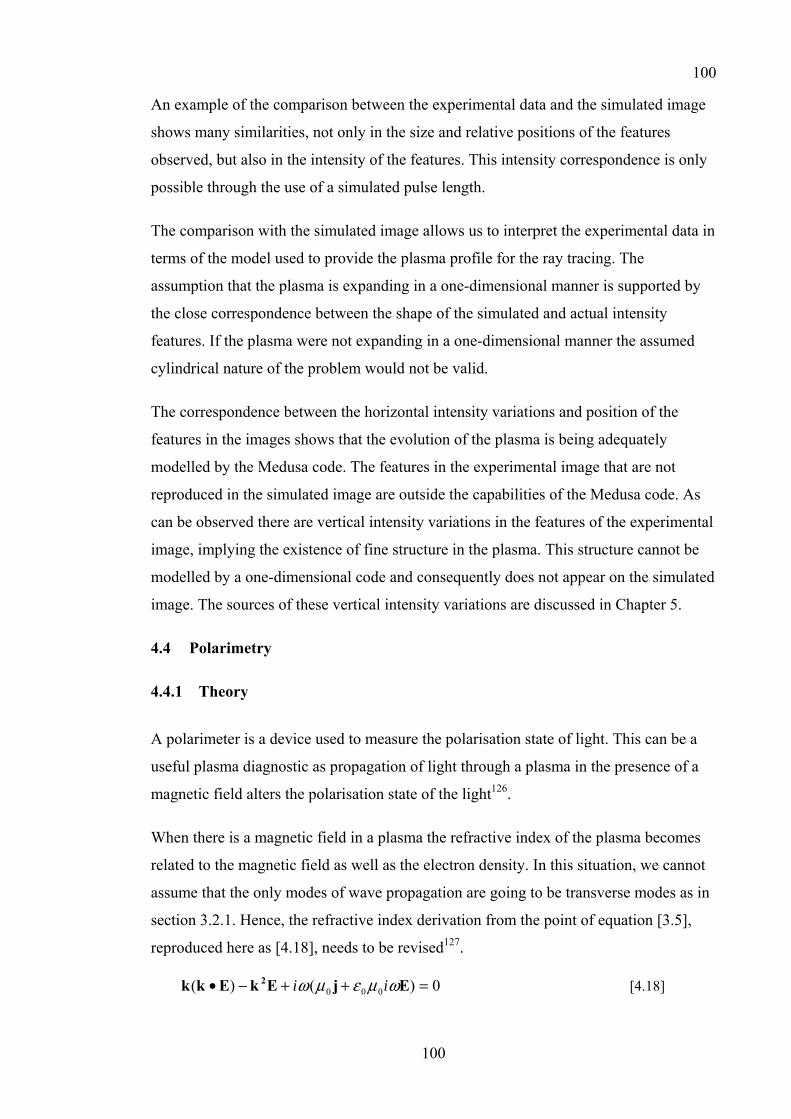
100
100
An example of the comparison between the experimental data and the simulated image
shows many similarities, not only in the size and relative positions of the features
observed, but also in the intensity of the features. This intensity correspondence is only
possible through the use of a simulated pulse length.
The comparison with the simulated image allows us to interpret the experimental data in
terms of the model used to provide the plasma profile for the ray tracing. The
assumption that the plasma is expanding in a one-dimensional manner is supported by
the close correspondence between the shape of the simulated and actual intensity
features. If the plasma were not expanding in a one-dimensional manner the assumed
cylindrical nature of the problem would not be valid.
The correspondence between the horizontal intensity variations and position of the
features in the images shows that the evolution of the plasma is being adequately
modelled by the Medusa code. The features in the experimental image that are not
reproduced in the simulated image are outside the capabilities of the Medusa code. As
can be observed there are vertical intensity variations in the features of the experimental
image, implying the existence of fine structure in the plasma. This structure cannot be
modelled by a one-dimensional code and consequently does not appear on the simulated
image. The sources of these vertical intensity variations are discussed in Chapter 5.
4.4 Polarimetry
4.4.1 Theory
A polarimeter is a device used to measure the polarisation state of light. This can be a
useful plasma diagnostic as propagation of light through a plasma in the presence of a
magnetic field alters the polarisation state of the light126.
When there is a magnetic field in a plasma the refractive index of the plasma becomes
related to the magnetic field as well as the electron density. In this situation, we cannot
assume that the only modes of wave propagation are going to be transverse modes as in
section 3.2.1. Hence, the refractive index derivation from the point of equation [3.5],
reproduced here as [4.18], needs to be revised127.
0)()( 000 =++−• EjEkEkk 2 ωµεµω ii [4.18]

101
101
Where E is the electric field intensity vector, j is the total current density, µ0 is the
permeability of vacuum, ε0 is the permittivity of vacuum, k is the wave number and ω is
the angular frequency. If we treat the current as a linear function of the electric field,
from Ohm’s law we can write
),(),(),( ωωω kEkσkj •= [4.19]
Where σ is the conductivity tensor, which when combined with [4.18] leads to
0)(0
2
22 =⎟⎟
⎠
⎞⎜⎜⎝
⎛+•+−• EEσEEkk
ωεω ic
k [4.20]
Where c is the speed of light. As can be seen this leads to two types of solution, the
transverse case as derived previously in section 3.2.1 and a longitudinal case. However,
it is also correct to consider the conductivity of the plasma not only as an electric field
effect as in [3.10], but by also considering the force due to the external magnetic field.
Therefore, we should rewrite [3.10] as:
( )t
me e ∂∂=×+ e
evBvE 0 [4.21]
Where B0 is the external magnetic field, me is the mass of an electron, e is the
elementary charge and ve is the velocity of the electron. Assuming B0 is in the z
direction also we can also split the motion into components, in the knowledge that the
Fourier mode of E scales as exp(-iωt) : -
ω
ω
ω
ime
imeeim
ee
e
ze
e
eye
e
exe
z
x
y
y
x
−−
=
−+−
=
−
−−=
Ev
vBEv
vBEv
0
0
[4.22]
Solving these equations in terms of E gives solutions in terms of the electron gyro-
frequency, ωc, as defined in section 2.2.2
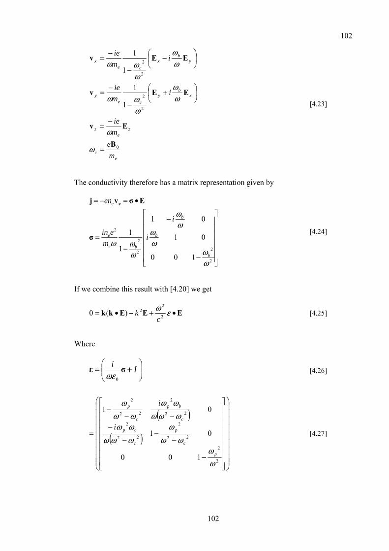
102
102
ec
ze
z
xb
yce
y
yb
xce
x
me
mie
imie
imie
0
2
2
2
2
1
1
1
1
B
Ev
EEv
EEv
=
−=
⎟⎠
⎞⎜⎝
⎛ +−
−=
⎟⎠
⎞⎜⎝
⎛ −−
−=
ω
ω
ωω
ωωω
ωω
ωωω
[4.23]
The conductivity therefore has a matrix representation given by
⎥⎥⎥⎥⎥⎥
⎦
⎤
⎢⎢⎢⎢⎢⎢
⎣
⎡
−
−
−=
•=−=
2
22
2
2
100
01
01
1
1
ωω
ωω
ωω
ωωω
b
b
b
be
e
e
i
i
mein
en
σ
Eσvj e
[4.24]
If we combine this result with [4.20] we get
EEEkk •+−•= εω2
22)(0
ck [4.25]
Where
⎟⎟⎠
⎞⎜⎜⎝
⎛+= Ii σε
0ωε [4.26]
( )
( )
⎟⎟⎟⎟⎟⎟⎟⎟⎟
⎠
⎞
⎜⎜⎜⎜⎜⎜⎜⎜⎜
⎝
⎛
⎥⎥⎥⎥⎥⎥⎥⎥
⎦
⎤
⎢⎢⎢⎢⎢⎢⎢⎢
⎣
⎡
−
−−
−
−−−
−
=
2
2
22
2
22
2
22
2
22
2
100
01
01
ωω
ωωω
ωωωωω
ωωωωω
ωωω
p
c
p
c
cp
c
bp
c
p
i
i
[4.27]
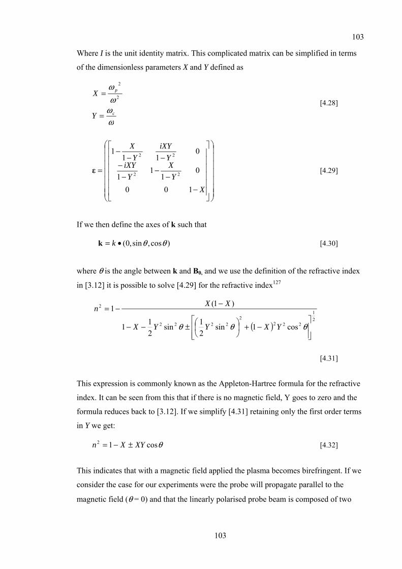
103
103
Where I is the unit identity matrix. This complicated matrix can be simplified in terms
of the dimensionless parameters X and Y defined as
ωωωω
c
p
Y
X
=
= 2
2
[4.28]
⎟⎟⎟⎟⎟⎟⎟
⎠
⎞
⎜⎜⎜⎜⎜⎜⎜
⎝
⎛
⎥⎥⎥⎥⎥⎥
⎦
⎤
⎢⎢⎢⎢⎢⎢
⎣
⎡
−−
−−
−−−
=
XY
XY
iXYY
iXYY
X
100
01
11
011
1
22
22
ε [4.29]
If we then define the axes of k such that
)cos,sin,0( θθ•= kk [4.30]
where θ is the angle between k and B0, and we use the definition of the refractive index
in [3.12] it is possible to solve [4.29] for the refractive index127
( )21
2222
2222
2
cos1sin21sin
211
)1(1
⎥⎥⎦
⎤
⎢⎢⎣
⎡−+⎟
⎠⎞
⎜⎝⎛±−−
−−=
θθθ YXYYX
XXn
[4.31]
This expression is commonly known as the Appleton-Hartree formula for the refractive
index. It can be seen from this that if there is no magnetic field, Y goes to zero and the
formula reduces back to [3.12]. If we simplify [4.31] retaining only the first order terms
in Y we get:
θcos12 XYXn ±−= [4.32]
This indicates that with a magnetic field applied the plasma becomes birefringent. If we
consider the case for our experiments were the probe will propagate parallel to the
magnetic field (θ = 0) and that the linearly polarised probe beam is composed of two

104
104
circularly polarised beams which propagate through the plasma with refractive indexes
of n+2=1-X+XY and n-
2=1-X-XY.
It can be seen that due to the difference between the two refractive indexes as the wave
propagates in z there will be a phase difference introduced between the two waves of:
zc
nn ωφ )( −+ −=∆ [4.33]
Hence there will be a change in the angle of polarisation by the process of Faraday
rotation, α, when the waves are superimposed of half the phase difference:
( )z
cX
XY ωφα⎥⎥
⎦
⎤
⎢⎢
⎣
⎡
−=∆=
21
121
2 [4.34]
If the plasma is well below critical density X tends to zero so this can be rewritten as
zcm
eB
e
p2
2
21
ωω
α = [4.35]
By substitution for the definition of the refractive index in terms of the electron density
in [3.13] and integrating [4.35] over a path in z we can write:
∫ •= dlBece
ncnm
e2
α [4.36]
Hence, from a measurement of the rotation of the angle of polarisation of the probe
beam and an interferometric measurement of the chord integrated electron density it is
possible to evaluate the magnetic field.
4.4.2 Polarimeter Designs
The diagnostic used to measure the polarisation state of the probe after propagation
through the plasma has to be a single shot device. For this reason a Wollaston prism is
used to separate the probe beam into two divergent, orthogonally polarised beams which
are imaged onto separate areas of a CCD detector.
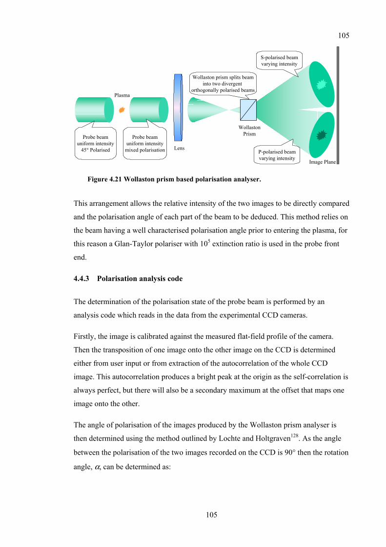
105
105
Lens
Plasma
WollastonPrism
S-polarised beamvarying intensity
P-polarised beamvarying intensity
Wollaston prism splits beaminto two divergent
orthogonally polarised beams
Probe beamuniform intensity
mixed polarisation
Probe beamuniform intensity
45° Polarised
Image Plane
Figure 4.21 Wollaston prism based polarisation analyser.
This arrangement allows the relative intensity of the two images to be directly compared
and the polarisation angle of each part of the beam to be deduced. This method relies on
the beam having a well characterised polarisation angle prior to entering the plasma, for
this reason a Glan-Taylor polariser with 105 extinction ratio is used in the probe front
end.
4.4.3 Polarisation analysis code
The determination of the polarisation state of the probe beam is performed by an
analysis code which reads in the data from the experimental CCD cameras.
Firstly, the image is calibrated against the measured flat-field profile of the camera.
Then the transposition of one image onto the other image on the CCD is determined
either from user input or from extraction of the autocorrelation of the whole CCD
image. This autocorrelation produces a bright peak at the origin as the self-correlation is
always perfect, but there will also be a secondary maximum at the offset that maps one
image onto the other.
The angle of polarisation of the images produced by the Wollaston prism analyser is
then determined using the method outlined by Lochte and Holtgraven128. As the angle
between the polarisation of the two images recorded on the CCD is 90° then the rotation
angle, α, can be determined as:

106
106
⎟⎟⎠
⎞⎜⎜⎝
⎛+−
= −
21
211sin21
IIIIα [4.37]
Where I1 and I2 are the intensities for corresponding elements of each image. It is
assumed that the sum of these two values is equal to the original intensity of the beam.
This assumption holds provided there is no significant amount of emission from the
plasma, and that the transmission of any optical components used in the diagnostic is
the same for both s and p polarised light. If there is emission from the plasma it should
be of random polarisation, and therefore should not effect the value of I1 – I2, but a
separate measurement of the original intensity of the beam is required.
If there is a difference in transmission of any optical components, calibration of the
diagnostic should enable this effect to be compensated for.
This analysis process is performed for each corresponding element of the two images
that can be mapped out. To increase the accuracy of the result at the expense of spatial
resolution, the intensities used can be taken from individual pixels, or the sum of a 3x3,
5x5, 7x7 or 9x9 rectangle centred around the pixel on a rolling average. For each
calculation that is performed, the statistical error in the calculation due to the random
counting error129 is evaluated. The accuracy of this technique is highest for comparable
values of I1 and I2, hence the initial input angle is set experimentally at 45 degrees.
The accuracy of the polarisation angle calculation improves with the number of events
counted, which directly relates to the dynamic resolution of the CCD cameras used.
This can be seen from the degree of numerical error in the calculation of [4.37] based on
the value of I1 + I2 being constant at 256 counts for an 8-bit CCD and 10,000 counts for
a 16-bit CCD as shown in Figure 4.22.
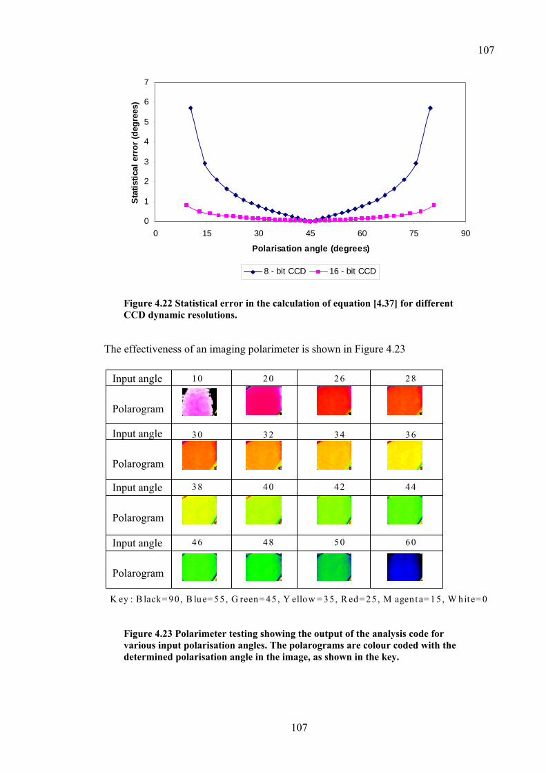
107
107
0
1
2
3
4
5
6
7
0 15 30 45 60 75 90
Polarisation angle (degrees)
Stat
istic
al e
rror
(deg
rees
)
8 - bit CCD 16 - bit CCD
Figure 4.22 Statistical error in the calculation of equation [4.37] for different CCD dynamic resolutions.
The effectiveness of an imaging polarimeter is shown in Figure 4.23
10 20 26 28
30 32 34 36
38 40 42 44
46 48 50 60
K ey : B lack= 90 , B lue= 55 , G reen= 45 , Y ellow = 35 , R ed= 25, M agent a= 15 , W hit e= 0
Figure 4.23 Polarimeter testing showing the output of the analysis code for various input polarisation angles. The polarograms are colour coded with the determined polarisation angle in the image, as shown in the key.
Input angle
Polarogram
Input angle
Polarogram
Input angle
Polarogram
Input angle
Polarogram
108
108
The input polarisation of the beam was set at the angle noted above each polarogram
using a sheet polariser with an extinction ratio of 103. The polarograms were generated
using an imaging analyser as described in Figure 4.21 and recorded on 8-bit CCD
cameras. As can be seen in Figure 4.23 the polarogram for an reference angle of 10
degrees shows significant amounts of magenta (equivalent to an angle of 15 degrees)
implying an error of approximately 5 degrees, whereas closer to 45 degrees the apparent
error is less an 1 degree. This would appear to validate the error curve for this
arrangement in Figure 4.22.
In the experiment, 16-bit CCD cameras were used to improve the sensitivity of the
diagnostic. From the calculation of the angle of rotation, with the experimental
conditions of a density of around 1019 cm-3 and a 10T magnetic field and a propagation
distance of 1mm a rotation of 0.041 degrees would be predicted. The statistical error in
such a measurement would be 0.0003 degrees. However, the level of background self-
emission from the plasma at the probe intensity used was sufficient to limit the effective
accuracy of the diagnostic to +/- 0.1 degrees. In light of this, the polarimetry diagnostic
was to be used to measure the amount of Faraday rotation introduced by the
experimental magnetic field when the probe propagated through a 1mm thick piece of
SF57 glass.
4.5 Conclusions
In this chapter, I have presented diagnostic methods for measuring the electron density
and magnetic field structure in a plasma and for observing the electron density gradient
in a plasma. This has been achieved through a discussion of the theory behind, and
experimental designs used for Interferometery, Schlieren Imaging, Shadowgraphy and
Polarimetry diagnostics. I have also discussed the analysis techniques used to interpret
the experimental data produced by these diagnostics. This has included the development
of computational tools to assist the analysis. For the analysis of interferometric data, a
code has been developed which enables the extraction of small fringe shifts in the data
more accurately than by eye. The extracted data can also be used in conjunction with an
Abel inversion routine to study the internal structure of cylindrically symmetric plasma.
To assist in the interpretation of Schlieren images an iterative ray tracing code was
developed, which is in agreement with published analytical ray tracing solutions125. This

109
109
code can be used to compare the experimental data with numerical simulations of the
plasma by producing simulated schlieren images.
The analysis of polarimetry data where both s and p polarised images are formed on a
single CCD can be performed automatically using a third code. The transposition
between the s and p polarised images can be determined through autocorrelation or by
user defined input. The polarisation angle is calculated for each point in the image along
with an estimation of the statistical error in the calculation.
110
110
5 Chapter 5 - Producing plasma from a single thin foil
5.1 Introduction
In this chapter the production and characterisation of laser-exploded thin films is
described. The production of a plasma from a thin film by direct laser irradiation is well
established technique and used in many types laser plasma experiments, including X-
ray laser production130, hydrodynamic instability studies131,132 and colliding plasma
inter-penetration experiments133. The definition of thin foil thickness changes depending
on the experiment, in some cases these foils are around a few microns thick, in our case
the foil thickness is typically 100 nm.
These thin foils are necessary as high expansion velocities (>107 cms-1) and low
densities (~1018 cm-3) are required to ensure the interaction between two similar foils in
a colliding geometry is collisionless. This collisionless interaction is discussed in the
next chapter.
Plasma formation from exploding thin foils is sensitive to laser beam intensity non-
uniformity across the focal spot, and the presence of target imperfections in terms of
thickness and density, and surface structures, which density uniformity in the expanding
plasma. To use exploding plasmas for scaled astrophysical simulations it is important to
ensure the plasma is uniform. This is to ensure that the physical processes of interest are
not masked by a highly structured plasma. Furthermore, a clear understanding of the
parameters of the exploding plasma is required before studying the more complex
situation of colliding plasma experiments.
In this chapter I will begin by describing the experimental technique used to produce an
exploding plasma, including how the plasma is diagnosed, and then present data
showing spatial and time resolved measurements of the subsequent expansion. This
experimental data is compared with both an analytical model and numerical simulation
of the plasma.
Density non-uniformities are present in the exploding plasmas and are observed to
persist through the expansion. Sources of plasma non-uniformity are described,
including a discussion of target quality, and then I shall demonstrate that by varying the

111
111
laser focal spot intensity profile that at least part of the observed density non-
uniformities result from the intensity structure in the focal spot. I will introduce the
concept of pre-pulse smoothing and present experimental evidence for the success of
this innovative technique before drawing conclusions.
5.2 Experimental technique
5.2.1 Introduction
These experiments were conducted at the Central Laser Facility using the VULCAN134
laser and Target Area East. The experiments and results described in this chapter were
conducted as part of three colliding plasma experiments conducted during 2000, 2001
and 2002. In the following sub-sections target design, manufacture and the experimental
target area configuration are described.
5.2.2 Target Design and Manufacture
Target design was dictated by the need to produce uniform, large area plasmas suitable
for studying collisionless plasma physics on a kilo-Joule scale laser such as Vulcan.
Laser energy limitations, and Medusa simulations, suggested 1 mm diameter 100 nm
thick foils would produce a rapidly expanding one-dimensional plasma with densities
and dimensions suitable for optical probing. In addition, the target and the holders
needed to be sufficiently small so that they would easily fit in to a mm-scale Helmholtz
coil. These Helmholtz coils are described in Chapter 6.
The target holders were manufactured either by punching them from 250µm thick mylar
sheets or from 50µm thick photo-etched copper. In both cases the holder geometry was
the same, an 8mm by 2mm rectangle with a 1.2mm diameter hole centred 1mm from
one end as shown in Figure 5.1. The thin foils are mounted across the 1.2mm diameter
hole.
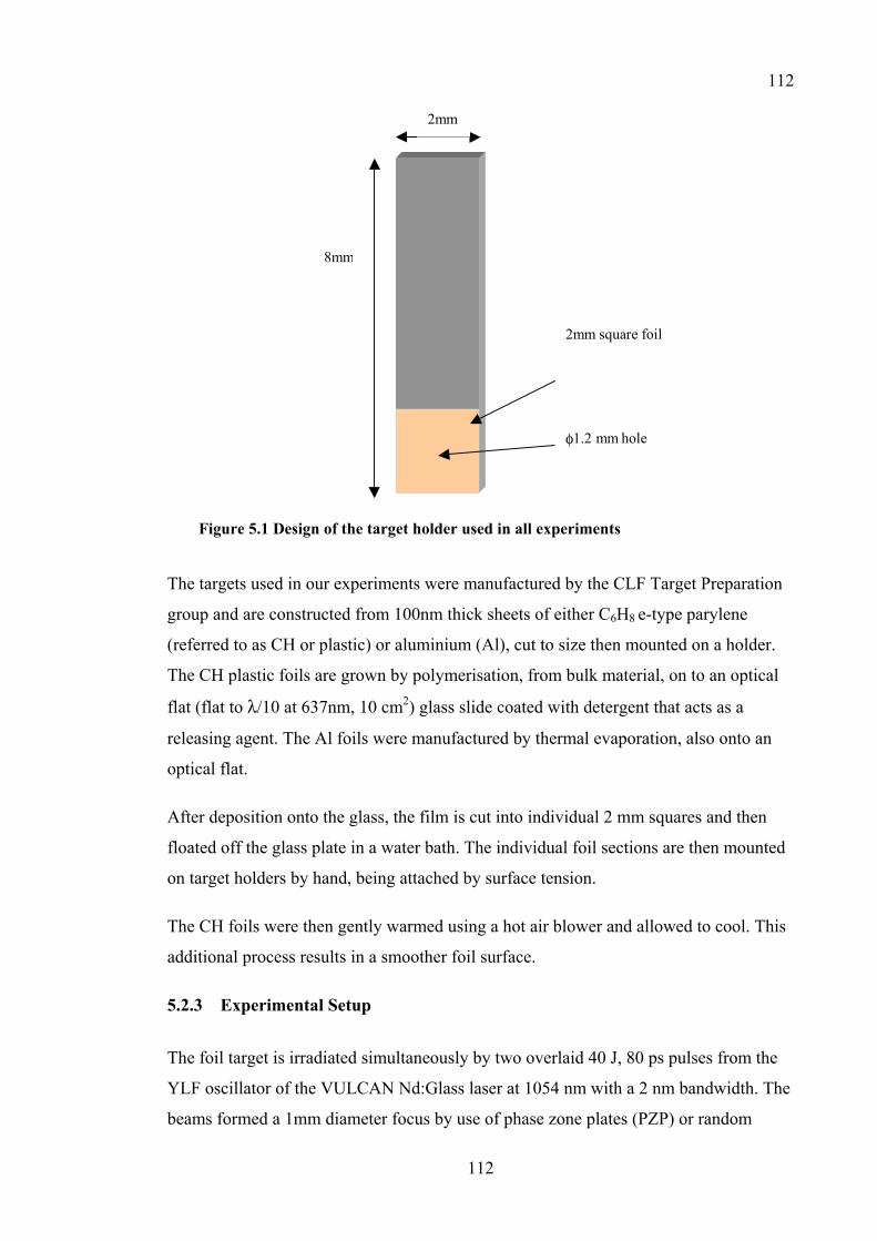
112
112
2mm square foil
8mm
φ1.2 mm hole
2mm
Figure 5.1 Design of the target holder used in all experiments
The targets used in our experiments were manufactured by the CLF Target Preparation
group and are constructed from 100nm thick sheets of either C6H8 e-type parylene
(referred to as CH or plastic) or aluminium (Al), cut to size then mounted on a holder.
The CH plastic foils are grown by polymerisation, from bulk material, on to an optical
flat (flat to λ/10 at 637nm, 10 cm2) glass slide coated with detergent that acts as a
releasing agent. The Al foils were manufactured by thermal evaporation, also onto an
optical flat.
After deposition onto the glass, the film is cut into individual 2 mm squares and then
floated off the glass plate in a water bath. The individual foil sections are then mounted
on target holders by hand, being attached by surface tension.
The CH foils were then gently warmed using a hot air blower and allowed to cool. This
additional process results in a smoother foil surface.
5.2.3 Experimental Setup
The foil target is irradiated simultaneously by two overlaid 40 J, 80 ps pulses from the
YLF oscillator of the VULCAN Nd:Glass laser at 1054 nm with a 2 nm bandwidth. The
beams formed a 1mm diameter focus by use of phase zone plates (PZP) or random
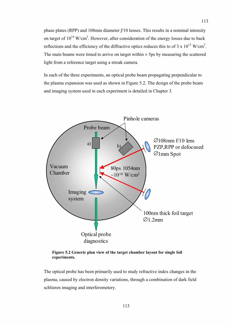
113
113
phase plates (RPP) and 108mm diameter f/10 lenses. This results in a nominal intensity
on target of 1014 W/cm2. However, after consideration of the energy losses due to back
reflections and the efficiency of the diffractive optics reduces this to of 3 x 10¹³ W/cm2.
The main beams were timed to arrive on target within ± 5ps by measuring the scattered
light from a reference target using a streak camera.
In each of the three experiments, an optical probe beam propagating perpendicular to
the plasma expansion was used as shown in Figure 5.2. The design of the probe beam
and imaging system used in each experiment is detailed in Chapter 3.
Probe beam
∅108mm f/10 lensPZP,RPP or defocused∅1mm Spot
Imagingsystem
80ps 1054nm~1014 W/cm2
Pinhole cameras
Optical probediagnostics
100nm thick foil target∅1.2mm
a) b)
VacuumChamber
Figure 5.2 Generic plan view of the target chamber layout for single foil experiments.
The optical probe has been primarily used to study refractive index changes in the
plasma, caused by electron density variations, through a combination of dark field
schlieren imaging and interferometery.
114
114
An interferometer was used during the third experiment, which was a modified
Normarski interferometer as described in section 4.2, imaged onto a 16 bit Andor CCD
with 13 µm square cells. The interferometer was adjusted to produce a reference fringe
pattern with 1 fringe approximately every 10 pixels.
The schlieren images were formed using 500mm focal length f/10 achromatic lenses
and 1.1mm or 1.6mm diameter stops, as described in section 4.3. The resolution of the
schlieren images is governed by the imaging optics and camera combination, which is
discussed in Chapter 3.
The X-ray emission from the foils was monitored using two Pulnix 8-bit CCD X-ray
pinhole cameras mounted inside the target chamber in the second experiment. These
cameras were set to image X-ray emission from the foil with camera a) perpendicular to
the foil, at x3 magnification, and camera b) at 37.5° to the foil surface normal at x5
magnification.
A second optical imaging system was employed to study the scattered focal spot
structure on the foil surface. The scattered light was imaged onto a 16 bit CCD camera,
as shown in Figure 5.3. This imaging system is identical to the one described for the
second experiment in Chapter 3.

115
115
f/10 lensPZP or RPP∅1mm Spot
80ps 1054nm1014 W/cm2
f/2.5f/10
16bit CCD
Focal spot imaging
100nm thick foil target∅1.2mm
Figure 5.3 Focal spot imaging system to study the west foil spot profile during the second experiment.
These focal spot measurements are time integrated, and resolution limited by the 27µm
CCD cell size rather than the optics.
5.3 Results
In this section, I will describe the measurement of the expansion speed, the electron
density profile and the non-uniform structure of the plasma. I will then report the
measurements of the possible sources of these non-uniform structures through
measurements of the laser focal spot profile and the characterisation of the targets.
5.3.1 Expansion
The expansion velocity of the plasma is inferred from the interferograms by locating the
point of furthest detectable fringe shift attributable to the plasma. This process was
performed using the automatically extracted phase shift map, which as described in
section 4.2.3 has the advantage of accurately detecting small fringe shifts. However,
there is still an element of noise in the extracted data introducing an error in locating
this position of +/- 10 pixels. The distances from the foil’s initial position to the leading
edge are plotted against the elapsed time in Figure 5.4.

116
116
0
100
200
300
400
500
600
700
800
900
1000
0 100 200 300 400 500 600 700 800
Time (ps)
Dis
tanc
e (m
icro
ns)
1.55 microns/ps1.3 microns/ps1.13 microns/ps1.51 microns/ps
Figure 5.4 Graph of plasma expansion, showing expansion up to 500 ps at 1.55 µm/ps and up to 750 ps at 1.3 µm/ps
The velocity of the leading edge is assumed to be constant over the expansion. There
may be a residual error in the assumed position of the initial foil surface, hence the
velocities are calculated both assuming the line passes through zero (solid lines) and
linear best fit to the data (dashed lines).
At 750 ps as the plasma density is decreasing during the expansion the leading edge cut
off may have dropped below the sensitivity of the interferometer at this time, making
the later measurements less accurate. Also once the plasma has expanded beyond
500µm the expansion is can longer be considered one-dimensional. For this reason, the
velocity is deduced with this data point (blue lines) and without (purple lines). The
velocities for the expansion up to 500ps provide a good match to a constant velocity,
within the error of the measurement, with only a small correction for the potential
misplacement of the initial foil position. The 750ps data point appears to be erroneous,
as the linear fit falls outside the error of the measurements, and does not fit well with
the zero point. This supports the concept of a one-dimensional expansion up to 500µm
from the foil surface.
117
117
5.3.2 Density Profile
The determination of the electron density profile by provides details of the evolution of
the plasma without perturbing its structure. It also allows us to study the internal radial
structure of the plasma through Abel inversion of interferometric data, as described in
section 4.2.4. This type of measurement is important as it directly provides quantitative
plasma parameter data.
Electron density profiles have been measured for various points in the evolution of a
thin foil plasma by varying the relative delay of the optical probe beam on a timing
slide. Interference patterns were recorded between 250 ps and 1500 ps after the main
drive beams are presented in Figure 5.5.
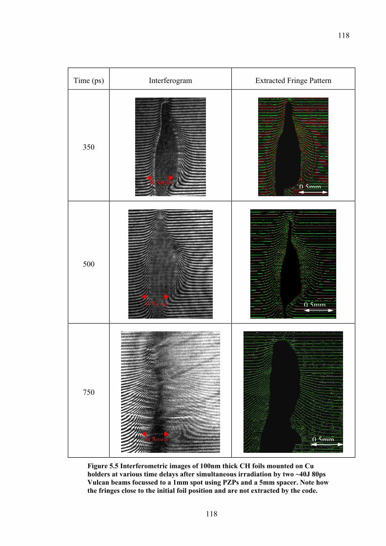
118
118
Time (ps) Interferogram Extracted Fringe Pattern
350
500
750
Figure 5.5 Interferometric images of 100nm thick CH foils mounted on Cu holders at various time delays after simultaneous irradiation by two ~40J 80ps Vulcan beams focussed to a 1mm spot using PZPs and a 5mm spacer. Note how the fringes close to the initial foil position and are not extracted by the code.
0 5mm
0 5mm
0 5mm
0 5mm
0 5mm
0 5mm
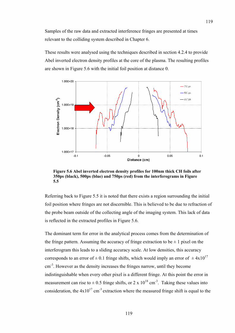
119
119
Samples of the raw data and extracted interference fringes are presented at times
relevant to the colliding system described in Chapter 6.
These results were analysed using the techniques described in section 4.2.4 to provide
Abel inverted electron density profiles at the core of the plasma. The resulting profiles
are shown in Figure 5.6 with the initial foil position at distance 0.
Figure 5.6 Abel inverted electron density profiles for 100nm thick CH foils after 350ps (black), 500ps (blue) and 750ps (red) from the interferograms in Figure 5.5
Referring back to Figure 5.5 it is noted that there exists a region surrounding the initial
foil position where fringes are not discernible. This is believed to be due to refraction of
the probe beam outside of the collecting angle of the imaging system. This lack of data
is reflected in the extracted profiles in Figure 5.6.
The dominant term for error in the analytical process comes from the determination of
the fringe pattern. Assuming the accuracy of fringe extraction to be ± 1 pixel on the
interferogram this leads to a sliding accuracy scale. At low densities, this accuracy
corresponds to an error of ± 0.1 fringe shifts, which would imply an error of ± 4x10¹⁷
cm-3. However as the density increases the fringes narrow, until they become
indistinguishable when every other pixel is a different fringe. At this point the error in
measurement can rise to ± 0.5 fringe shifts, or 2 x 1018 cm-3. Taking these values into
consideration, the 4x1017 cm-3 extraction where the measured fringe shift is equal to the

120
120
potential for error the error itself is ±100%. However at the highest densities measured
at ~3x1019 cm-3 the maximum measurement error is only ±6%.
5.3.3 Plasma non-uniformity
An interesting feature observed in the interferometer data is the onset of non-
uniformities in the expanding foil. These can be seen to develop as filaments, which are
first noticeable after 350ps in Figure 5.5 and have been observed in other
experiments135. After 750ps, the distortion caused by the filamentation of the plasma is
quite distinct in the fringe pattern.
Evidence of plasma non-uniformity has been observed in all three experiments. Results
supporting the presence of non-uniformity come mainly from the dark field schlieren
imaging diagnostic as described in section 4.3.
The schlieren images provide a measurement of the scale lengths of the structures that
can be seen, although it is not possible to directly infer the magnitude of the electron
density gradient structure. In this case the measurement is limited only by the resolution
of the optical probe system, which is discussed for each experiment in Chapter 3. In a
uniform thin foil plasma each plasma should produce a schlieren image with two
vertical features, one either side of the target holder. No horizontal structures are
expected from uniform plasma, as is shown by the ray tracing simulations in section
4.3.4.
The results from the first experiment136 showed significant amounts of horizontal
structure in the schlieren images, as shown in Figure 5.7. These structures are observed
to change as the focussing conditions of the laser are altered.
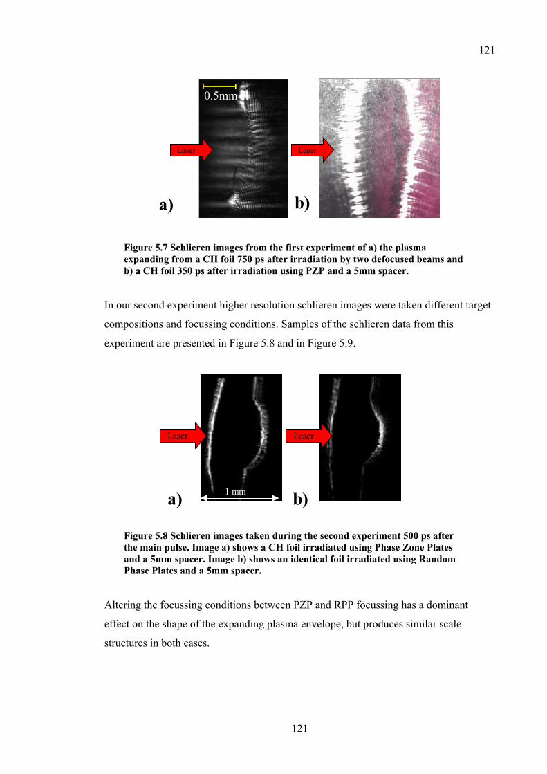
121
121
a) b)
0.5mm
Laser Laser
Figure 5.7 Schlieren images from the first experiment of a) the plasma expanding from a CH foil 750 ps after irradiation by two defocused beams and b) a CH foil 350 ps after irradiation using PZP and a 5mm spacer.
In our second experiment higher resolution schlieren images were taken different target
compositions and focussing conditions. Samples of the schlieren data from this
experiment are presented in Figure 5.8 and in Figure 5.9.
a) b)1 mm
Laser Laser
Figure 5.8 Schlieren images taken during the second experiment 500 ps after the main pulse. Image a) shows a CH foil irradiated using Phase Zone Plates and a 5mm spacer. Image b) shows an identical foil irradiated using Random Phase Plates and a 5mm spacer.
Altering the focussing conditions between PZP and RPP focussing has a dominant
effect on the shape of the expanding plasma envelope, but produces similar scale
structures in both cases.
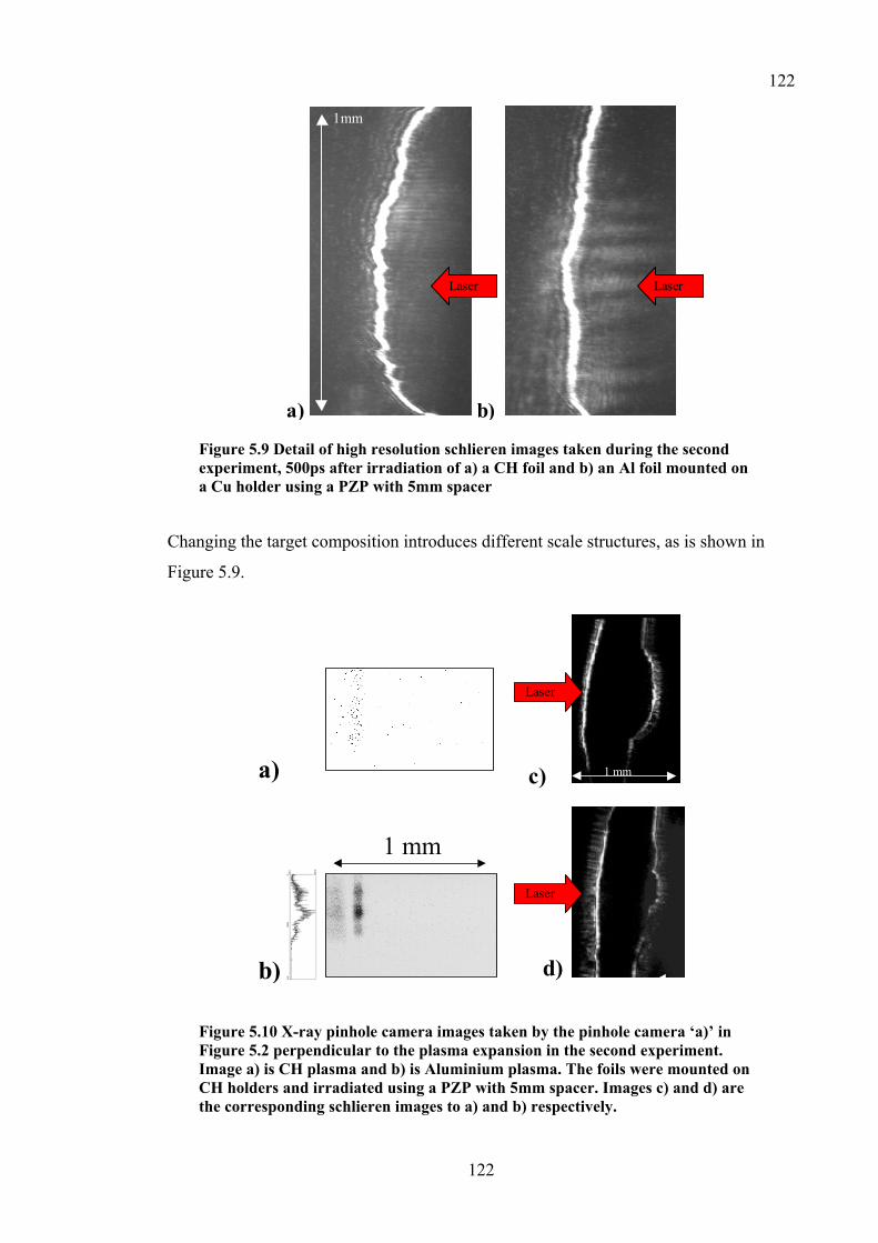
122
122
a) b)
Laser Laser
1mm
Figure 5.9 Detail of high resolution schlieren images taken during the second experiment, 500ps after irradiation of a) a CH foil and b) an Al foil mounted on a Cu holder using a PZP with 5mm spacer
Changing the target composition introduces different scale structures, as is shown in
Figure 5.9.
1 mm
a)
b)
c)
d)
1 mm
Laser
Laser
Figure 5.10 X-ray pinhole camera images taken by the pinhole camera ‘a)’ in Figure 5.2 perpendicular to the plasma expansion in the second experiment. Image a) is CH plasma and b) is Aluminium plasma. The foils were mounted on CH holders and irradiated using a PZP with 5mm spacer. Images c) and d) are the corresponding schlieren images to a) and b) respectively.
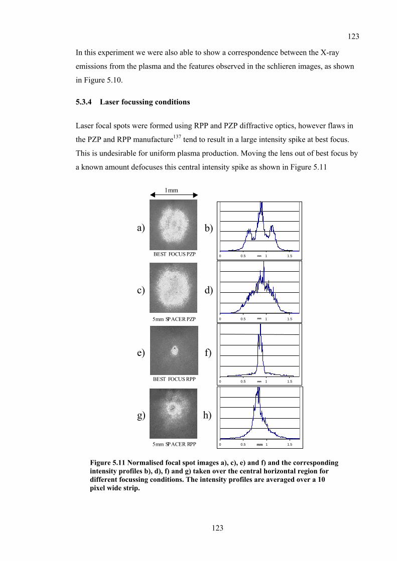
123
123
In this experiment we were also able to show a correspondence between the X-ray
emissions from the plasma and the features observed in the schlieren images, as shown
in Figure 5.10.
5.3.4 Laser focussing conditions
Laser focal spots were formed using RPP and PZP diffractive optics, however flaws in
the PZP and RPP manufacture137 tend to result in a large intensity spike at best focus.
This is undesirable for uniform plasma production. Moving the lens out of best focus by
a known amount defocuses this central intensity spike as shown in Figure 5.11
0 0.5 1 1.5mm5mm SPACER PZP
BEST FOCUS PZP
0 0.5 1 1.5mm
0 0.5 1 1.5mm5mm SPACER RPP
BEST FOCUS RPP
0 0.5 1 1.5mm
a) b)
c) d)
e) f)
g) h)
1mm
Figure 5.11 Normalised focal spot images a), c), e) and f) and the corresponding intensity profiles b), d), f) and g) taken over the central horizontal region for different focussing conditions. The intensity profiles are averaged over a 10 pixel wide strip.
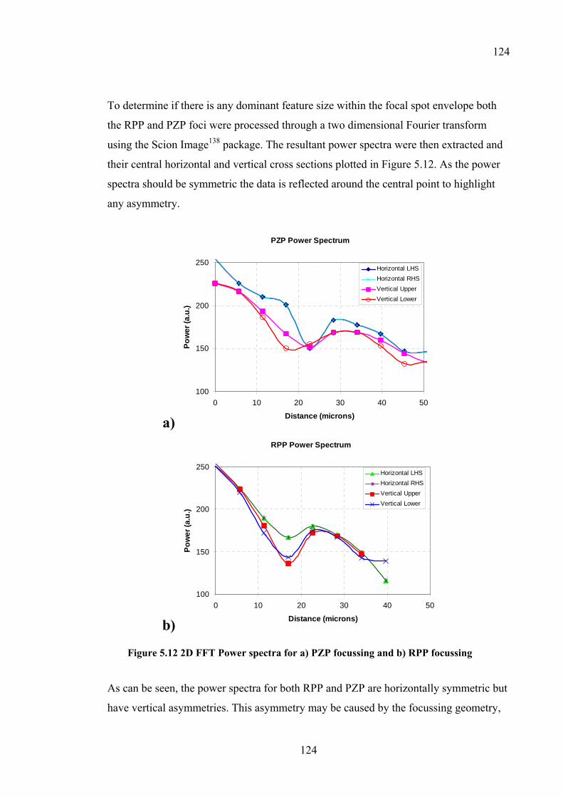
124
124
To determine if there is any dominant feature size within the focal spot envelope both
the RPP and PZP foci were processed through a two dimensional Fourier transform
using the Scion Image138 package. The resultant power spectra were then extracted and
their central horizontal and vertical cross sections plotted in Figure 5.12. As the power
spectra should be symmetric the data is reflected around the central point to highlight
any asymmetry.
a)
PZP Power Spectrum
100
150
200
250
0 10 20 30 40 50
Distance (microns)
Pow
er (a
.u.)
Horizontal LHSHorizontal RHSVertical UpperVertical Lower
b)
RPP Power Spectrum
100
150
200
250
0 10 20 30 40 50
Distance (microns)
Pow
er (a
.u.)
Horizontal LHSHorizontal RHSVertical UpperVertical Lower
Figure 5.12 2D FFT Power spectra for a) PZP focussing and b) RPP focussing
As can be seen, the power spectra for both RPP and PZP are horizontally symmetric but
have vertical asymmetries. This asymmetry may be caused by the focussing geometry,
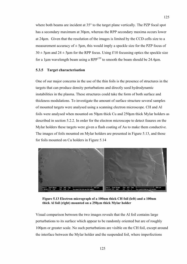
125
125
where both beams are incident at 35° to the target plane vertically. The PZP focal spot
has a secondary maximum at 30µm, whereas the RPP secondary maxima occurs lower
at 24µm. Given that the resolution of the images is limited by the CCD cells size to a
measurement accuracy of ± 5µm, this would imply a speckle size for the PZP focus of
30 ± 5µm and 24 ± 5µm for the RPP focus. Using f/10 focussing optics the speckle size
for a 1µm wavelength beam using a RPP139 to smooth the beam should be 24.4µm.
5.3.5 Target characterisation
One of our major concerns in the use of the thin foils is the presence of structures in the
targets that can produce density perturbations and directly seed hydrodynamic
instabilities in the plasma. These structures could take the form of both surface and
thickness modulations. To investigate the amount of surface structure several samples
of mounted targets were analysed using a scanning electron microscope. CH and Al
foils were analysed when mounted on 50µm thick Cu and 250µm thick Mylar holders as
described in section 5.2.2. In order for the electron microscope to detect feaures on the
Mylar holders these targets were given a flash coating of Au to make them conductive.
The images of foils mounted on Mylar holders are presented in Figure 5.13, and those
for foils mounted on Cu holders in Figure 5.14
Figure 5.13 Electron micrograph of a 100nm thick CH foil (left) and a 100nm thick Al foil (right) mounted on a 250µm thick Mylar holder
Visual comparison between the two images reveals that the Al foil contains large
perturbations to its surface which appear to be randomly oriented but are of roughly
100µm or greater scale. No such perturbations are visible on the CH foil, except around
the interface between the Mylar holder and the suspended foil, where imperfections
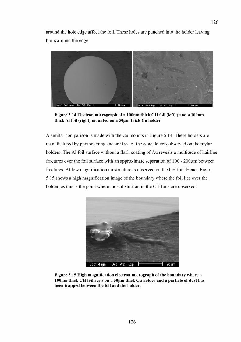
126
126
around the hole edge affect the foil. These holes are punched into the holder leaving
burrs around the edge.
Figure 5.14 Electron micrograph of a 100nm thick CH foil (left) ) and a 100nm thick Al foil (right) mounted on a 50µm thick Cu holder
A similar comparison is made with the Cu mounts in Figure 5.14. These holders are
manufactured by photoetching and are free of the edge defects observed on the mylar
holders. The Al foil surface without a flash coating of Au reveals a multitude of hairline
fractures over the foil surface with an approximate separation of 100 - 200µm between
fractures. At low magnification no structure is observed on the CH foil. Hence Figure
5.15 shows a high magnification image of the boundary where the foil lies over the
holder, as this is the point where most distortion in the CH foils are observed.
Figure 5.15 High magnification electron micrograph of the boundary where a 100nm thick CH foil rests on a 50µm thick Cu holder and a particle of dust has been trapped between the foil and the holder.
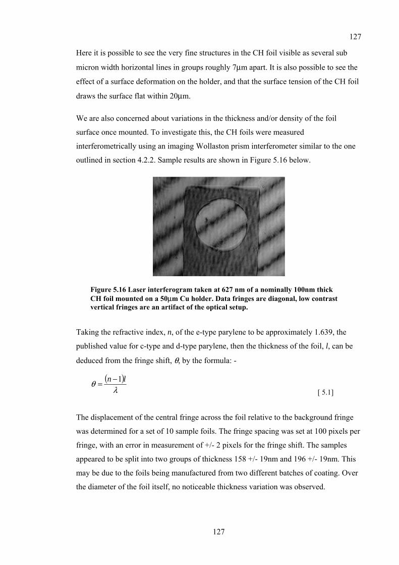
127
127
Here it is possible to see the very fine structures in the CH foil visible as several sub
micron width horizontal lines in groups roughly 7µm apart. It is also possible to see the
effect of a surface deformation on the holder, and that the surface tension of the CH foil
draws the surface flat within 20µm.
We are also concerned about variations in the thickness and/or density of the foil
surface once mounted. To investigate this, the CH foils were measured
interferometrically using an imaging Wollaston prism interferometer similar to the one
outlined in section 4.2.2. Sample results are shown in Figure 5.16 below.
Figure 5.16 Laser interferogram taken at 627 nm of a nominally 100nm thick CH foil mounted on a 50µm Cu holder. Data fringes are diagonal, low contrast vertical fringes are an artifact of the optical setup.
Taking the refractive index, n, of the e-type parylene to be approximately 1.639, the
published value for c-type and d-type parylene, then the thickness of the foil, l, can be
deduced from the fringe shift, θ, by the formula: -
( )λ
θ ln 1−= [ 5.1]
The displacement of the central fringe across the foil relative to the background fringe
was determined for a set of 10 sample foils. The fringe spacing was set at 100 pixels per
fringe, with an error in measurement of +/- 2 pixels for the fringe shift. The samples
appeared to be split into two groups of thickness 158 +/- 19nm and 196 +/- 19nm. This
may be due to the foils being manufactured from two different batches of coating. Over
the diameter of the foil itself, no noticeable thickness variation was observed.
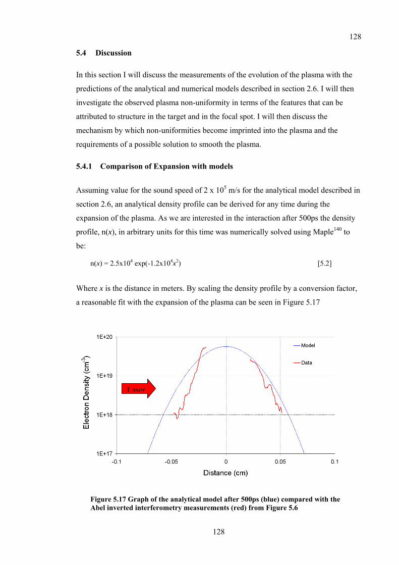
128
128
5.4 Discussion
In this section I will discuss the measurements of the evolution of the plasma with the
predictions of the analytical and numerical models described in section 2.6. I will then
investigate the observed plasma non-uniformity in terms of the features that can be
attributed to structure in the target and in the focal spot. I will then discuss the
mechanism by which non-uniformities become imprinted into the plasma and the
requirements of a possible solution to smooth the plasma.
5.4.1 Comparison of Expansion with models
Assuming value for the sound speed of 2 x 10⁵ m/s for the analytical model described in
section 2.6, an analytical density profile can be derived for any time during the
expansion of the plasma. As we are interested in the interaction after 500ps the density
profile, n(x), in arbitrary units for this time was numerically solved using Maple140 to
be:
n(x) = 2.5x10⁴ exp(-1.2x104x2) [5.2]
Where x is the distance in meters. By scaling the density profile by a conversion factor,
a reasonable fit with the expansion of the plasma can be seen in Figure 5.17
Figure 5.17 Graph of the analytical model after 500ps (blue) compared with the Abel inverted interferometry measurements (red) from Figure 5.6
Laser
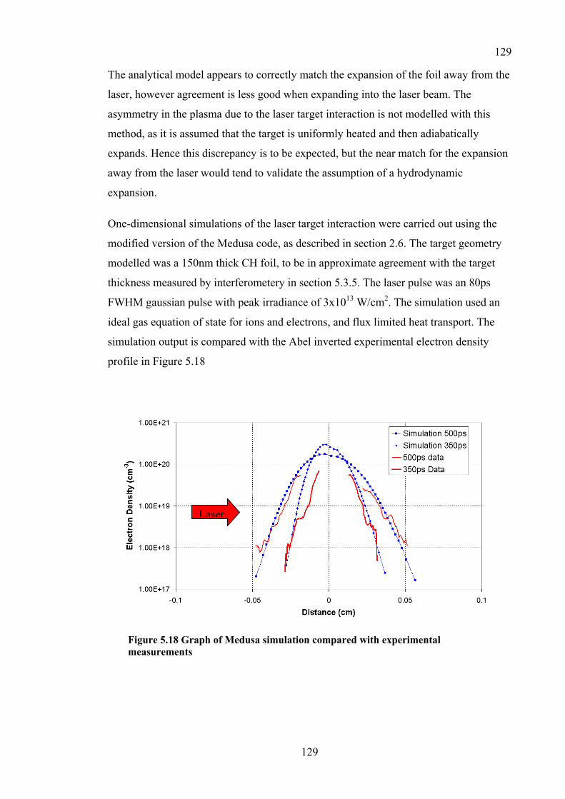
129
129
The analytical model appears to correctly match the expansion of the foil away from the
laser, however agreement is less good when expanding into the laser beam. The
asymmetry in the plasma due to the laser target interaction is not modelled with this
method, as it is assumed that the target is uniformly heated and then adiabatically
expands. Hence this discrepancy is to be expected, but the near match for the expansion
away from the laser would tend to validate the assumption of a hydrodynamic
expansion.
One-dimensional simulations of the laser target interaction were carried out using the
modified version of the Medusa code, as described in section 2.6. The target geometry
modelled was a 150nm thick CH foil, to be in approximate agreement with the target
thickness measured by interferometery in section 5.3.5. The laser pulse was an 80ps
FWHM gaussian pulse with peak irradiance of 3x10¹³ W/cm2. The simulation used an
ideal gas equation of state for ions and electrons, and flux limited heat transport. The
simulation output is compared with the Abel inverted experimental electron density
profile in Figure 5.18
Figure 5.18 Graph of Medusa simulation compared with experimental measurements
Laser

130
130
The simulation matches closely the evolution of the electron density profile up to the
point where the one-dimensional assumption becomes tenuous (where the expansion is
greater than half the target width).
The measured values of an expansion speed between 1.3 - 1.55x108 cm/s compare well
with Medusa simulation predictions of an expansion speed away from the laser of
1.46x108 cm/s.
5.4.2 Plasma non-uniformity
In the results gathered from the schlieren data we can separate the possible sources of
the non-uniformity into laser focus intensity profile and target structure. From an
analysis of the scale lengths of the structures observed in the schlieren images it is
possibly to deduce different forms of imprinting observed from both possible sources.
For this reason this section is split into a discussion of the target related features and the
laser related features.
5.4.2.1 Target structure
Evidence of plasma structure resulting from target non-uniformity can be most directly
be produced by comparing the scale of the features observed in the plasma with the
surface scans of the sample mounted targets. The first source of experimental evidence
for comparison is the schlieren image data. In interpreting schlieren images, it is
important to recall from section 4.3 that the dark field method is sensitive to electron
density gradients in any direction. Hence, a single density feature in the plasma would
present itself as two visible features on the schlieren. A comparison of the scale of
structure observed in CH and Al plasmas mounted on Cu holders and irradiated using
PZP focussing is shown in Figure 5.19.
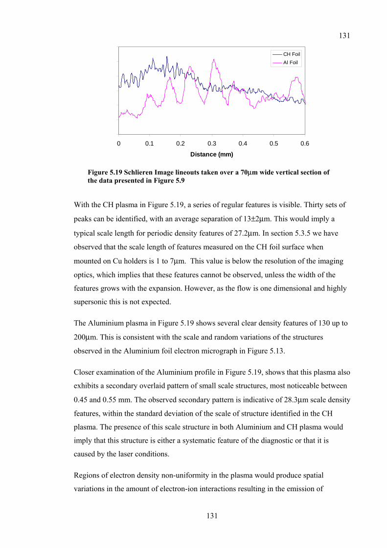
131
131
0
0
0
0
0
0
0
0 0.1 0.2 0.3 0.4 0.5 0.6
Distance (mm)
CH FoilAl Foil
Figure 5.19 Schlieren Image lineouts taken over a 70µm wide vertical section of the data presented in Figure 5.9
With the CH plasma in Figure 5.19, a series of regular features is visible. Thirty sets of
peaks can be identified, with an average separation of 13±2µm. This would imply a
typical scale length for periodic density features of 27.2µm. In section 5.3.5 we have
observed that the scale length of features measured on the CH foil surface when
mounted on Cu holders is 1 to 7µm. This value is below the resolution of the imaging
optics, which implies that these features cannot be observed, unless the width of the
features grows with the expansion. However, as the flow is one dimensional and highly
supersonic this is not expected.
The Aluminium plasma in Figure 5.19 shows several clear density features of 130 up to
200µm. This is consistent with the scale and random variations of the structures
observed in the Aluminium foil electron micrograph in Figure 5.13.
Closer examination of the Aluminium profile in Figure 5.19, shows that this plasma also
exhibits a secondary overlaid pattern of small scale structures, most noticeable between
0.45 and 0.55 mm. The observed secondary pattern is indicative of 28.3µm scale density
features, within the standard deviation of the scale of structure identified in the CH
plasma. The presence of this scale structure in both Aluminium and CH plasma would
imply that this structure is either a systematic feature of the diagnostic or that it is
caused by the laser conditions.
Regions of electron density non-uniformity in the plasma would produce spatial
variations in the amount of electron-ion interactions resulting in the emission of
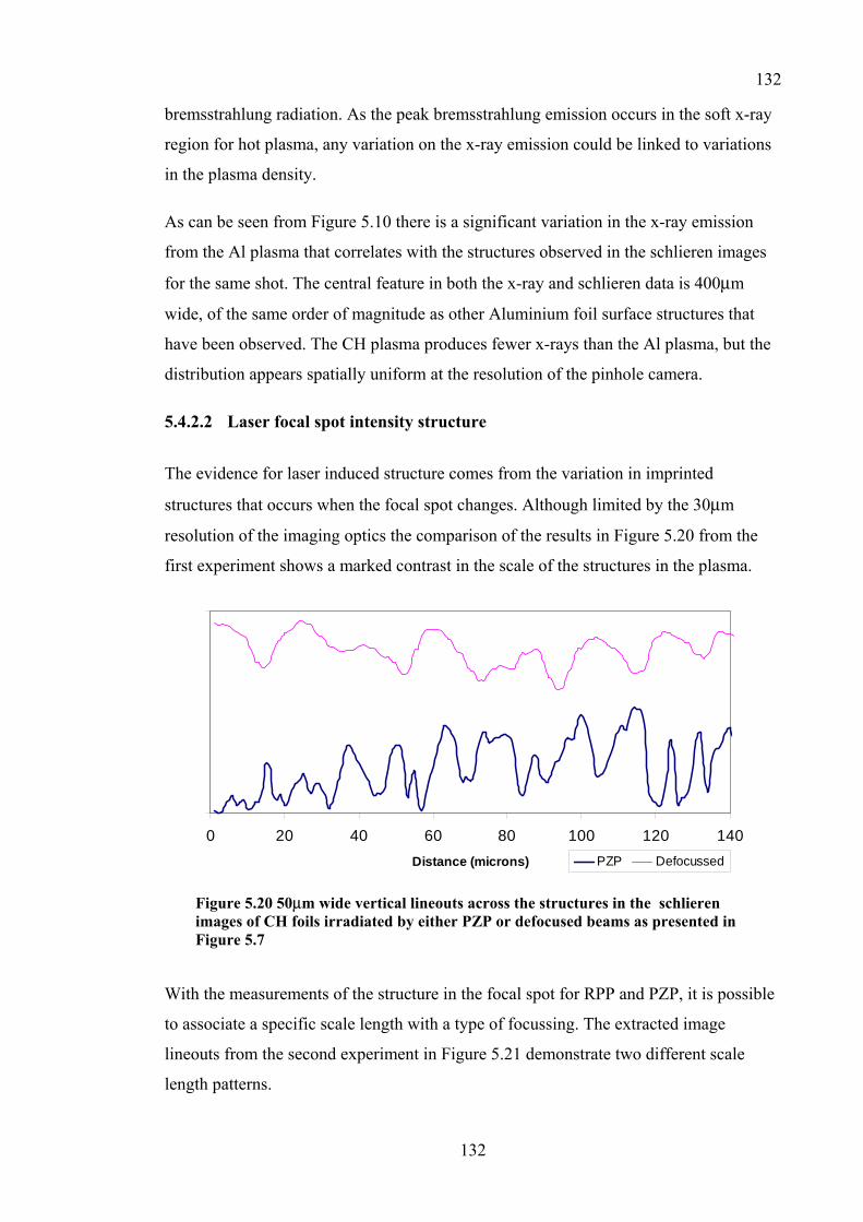
132
132
bremsstrahlung radiation. As the peak bremsstrahlung emission occurs in the soft x-ray
region for hot plasma, any variation on the x-ray emission could be linked to variations
in the plasma density.
As can be seen from Figure 5.10 there is a significant variation in the x-ray emission
from the Al plasma that correlates with the structures observed in the schlieren images
for the same shot. The central feature in both the x-ray and schlieren data is 400µm
wide, of the same order of magnitude as other Aluminium foil surface structures that
have been observed. The CH plasma produces fewer x-rays than the Al plasma, but the
distribution appears spatially uniform at the resolution of the pinhole camera.
5.4.2.2 Laser focal spot intensity structure
The evidence for laser induced structure comes from the variation in imprinted
structures that occurs when the focal spot changes. Although limited by the 30µm
resolution of the imaging optics the comparison of the results in Figure 5.20 from the
first experiment shows a marked contrast in the scale of the structures in the plasma.
0 20 40 60 80 100 120 140Distance (microns) PZP Defocussed
Figure 5.20 50µm wide vertical lineouts across the structures in the schlieren images of CH foils irradiated by either PZP or defocused beams as presented in Figure 5.7
With the measurements of the structure in the focal spot for RPP and PZP, it is possible
to associate a specific scale length with a type of focussing. The extracted image
lineouts from the second experiment in Figure 5.21 demonstrate two different scale
length patterns.
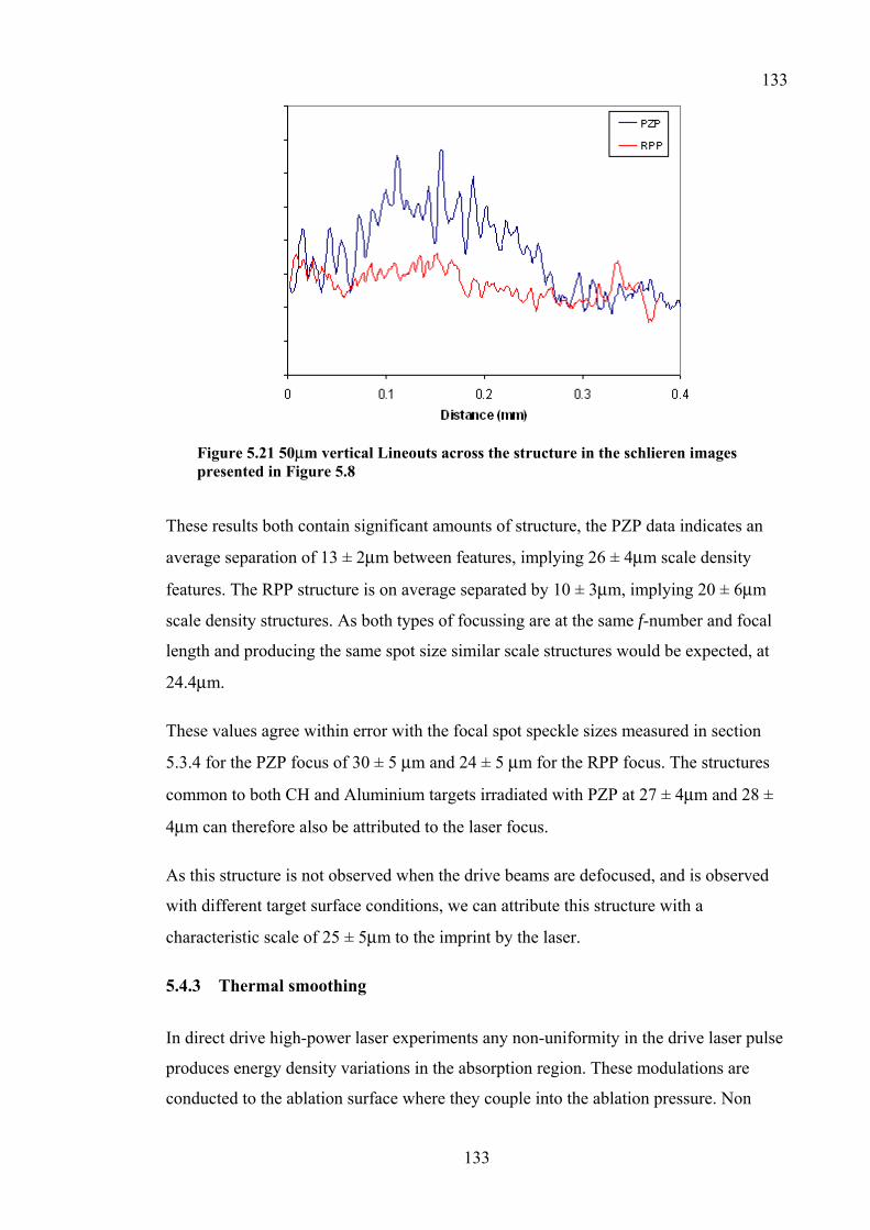
133
133
Figure 5.21 50µm vertical Lineouts across the structure in the schlieren images presented in Figure 5.8
These results both contain significant amounts of structure, the PZP data indicates an
average separation of 13 ± 2µm between features, implying 26 ± 4µm scale density
features. The RPP structure is on average separated by 10 ± 3µm, implying 20 ± 6µm
scale density structures. As both types of focussing are at the same f-number and focal
length and producing the same spot size similar scale structures would be expected, at
24.4µm.
These values agree within error with the focal spot speckle sizes measured in section
5.3.4 for the PZP focus of 30 ± 5 µm and 24 ± 5 µm for the RPP focus. The structures
common to both CH and Aluminium targets irradiated with PZP at 27 ± 4µm and 28 ±
4µm can therefore also be attributed to the laser focus.
As this structure is not observed when the drive beams are defocused, and is observed
with different target surface conditions, we can attribute this structure with a
characteristic scale of 25 ± 5µm to the imprint by the laser.
5.4.3 Thermal smoothing
In direct drive high-power laser experiments any non-uniformity in the drive laser pulse
produces energy density variations in the absorption region. These modulations are
conducted to the ablation surface where they couple into the ablation pressure. Non

134
134
uniform ablation pressure across the target surface at the onset of irradiation launches a
perturbed shock into the target. The rear surface of the target then becomes deformed by
the shock’s passing, producing “feed-in” perturbations141. In our experiments the targets
are so thin that the shock thickness is comparable with the target thickness, and no
“feed-in” perturbations are produced. This is supported by the accuracy of the analytical
model and hydrodynamic simulations in predicting the expansion of the plasma through
hydrodynamic expansion.
As material is ablated the non-uniform ablation pressure profile will be imprinted on the
plasma as it forms, generating “feed-through” perturbations141. The presence of a
plasma ‘atmosphere’ between the absorption region and the ablation surface allows
thermal diffusion to reduce these feed-through perturbations before they reach the
ablation surface. Both of these types of imprint perturbations in the plasma can seed
hydrodynamic instabilities and are a well-known problem for ICF experiments142.
The degree of feed-through perturbation that reaches the rear surface of the target can be
estimated by an evaluation of the amount of thermal smoothing that occurs. The
effectiveness of thermal smoothing has been shown to depend on the wavelength of the
laser143, the spatial scale of the imprinted modulations and the distance over which
smoothing occurs144. Experimental results for direct drive irradiation at 1054 nm and
1014 W/cm2 show that the degree of imprinting by the laser can be interpreted in terms
of [5.3]. Here a fractional change in ablation pressure p, due to a fractional change in
intensity I is smoothed by a factor n. This factor n is based on the spatial irregularities
in the focus of scale length L and the distance between the critical density surface and
the ablation front, D.
⎥⎦⎤
⎢⎣⎡−=→∆=∆
LDn
IIn
pp π4exp
[5.3]
As both the absorption region and the ablation surface are initially in contact at the front
surface of the target, the plasma that is produced from the front surface of the target is
always imprinted. Over time the distance D between the absorption region and the
ablation surface increases as the target ablates and non-uniform plasma is formed, until
this distance is sufficient for the diffusive thermal transport to homogenise the ablation
pressure. Optical smoothing techniques such as the use of Random Phase Plates145

135
135
(RPP) or Phase Zone Plates146 (PZP) improve the effectiveness of such thermal
smoothing by reducing the spatial scale of the intensity modulations in the focal spot.
Thereby also reducing the separation required between the absorption region and
ablation front for thermal smoothing to be effective. To illustrate the problem of
imprinting on very thin targets even using random phase plates to smooth the laser
beam we can consider the following example: -
For a 100 nm thick plastic foil target irradiated at 1012 W/cm2, Medusa simulations
show that the laser pulse would burn through the target in 13 ps. The distance between
the critical density surface and the ablation front is 0.37µm at this time. If these values
are substituted into [5.3] along with the theoretical speckle size of 24.4µm, then we get
a value for n of 0.82, meaning that virtually no thermal smoothing is occurring before
the target is completely ablated.
Hence, in the production of plasma from thin foils in our experiments, there is
insufficient target material to form a plasma atmosphere capable of effective smoothing
before the target has been completely ablated. This problem has been investigated using
radiatively heated low-density foam buffers before the target147. However, as our target
geometry is designed to match scaling criteria148 this experimental solution is not
suitable.
An experimental solution is required which allows the production of plasma from this
existing geometry without imprinting structures into the plasma produced from the rear
surface of the foil.
5.5 Plasma Smoothing experiment
Producing uniform plasma from thin foils would require a uniform laser focus in the
initial phase of irradiation. This has been achieved in 2002 using incoherent X-rays149,
however in our 2001 experiment we utilised a low energy pre-pulse, which is spatially
filtered immediately before the target.
The intention is to form an ablation surface with a uniform ablation pressure and,
providing there are no target surface structures, then pre-form a homogeneous
plasma.After the critical density surface has been separated from the ablation front, the
target can then be irradiated by non-uniform high energy drive beams, heating the

136
136
plasma and driving a supersonic hydrodynamic expansion. Without an ablation surface
to directly couple the laser non-uniformity into the plasma, imprinting on the plasma
formed at the rear surface of the foil should be limited.
Pre-pulse smoothing investigations were performed during the second experiment. In
the following sub-sections the experimental technique and results are presented, with a
discussion of the findings.
5.5.1 Experimental set up
100nm thick CH foil targets mounted on Cu holders were irradiated by a spatially
filtered pre pulse prior to irradiation by the main drive beams at 1014 W/cm2. Precise
measurements of the energy of the pre-pulse on target after the spatial filter were not
possible, however from calorimeter measurements of the pre-pulse beam prior to
entering the target chamber and estimated pinhole transmission, an on target intensity of
1013 W/cm2 is assumed.
f/10 lensPZP or RPP∅1mm Spot
50µm Pinholef/20 lens
17ps 1054nm
f/2.5
f/10
80ps 1054nm1014 W/cm2
Pinhole cameras15ps 527nm
Optical probe
100nm thick CH foil target∅1.2mm
1013 W/cm 2
Figure 5.22 Experimental chamber layout for pre-pulse experiments
137
137
The experimental arrangement was identical to that shown in Figure 5.2, with the
addition of a 50µm diameter pinhole mounted along the central axis of the foil, 20 mm
behind the target, as shown in Figure 5.22, and a CPA pre-pulse beam.
The pre-pulse for smoothing was derived from the same oscillator as the drive beams to
remove timing jitter. Measurements of the wave front quality of the pre-pulse beam150
show that it is at least 3 times the diffraction limit, therefore with a f/20 focus a 50µm
diameter pinhole is used for the spatial filter. Irradiating the pinhole with a high power
laser pulse will form plasma from the edge of the pinhole. We estimate that the
expansion of this plasma will prevent propagation of light through the pinhole after
10ps.
In order to deliver the maximum amount of energy through the pinhole a CPA pre-pulse
beam was compressed in air using a grating pair to a FWHM of 17±5 ps, in an identical
manner as described in chapter 3 for the optical probe. The combination of pulse
evolution and pinhole closure is designed provide optimum focal spot quality to
coincide with the peak intensity. The pre-pulse was focused onto the pinhole 20mm
from the target through a f/20 lens to generate a smooth 1mm focal spot on the foil. The
pre-pulse was designed to arrive up to 500 ps before the main drive beams, and
synchronised to within 5ps with the arrival of the main beams.
5.5.2 Results
High-resolution dark field schlieren images were taken of the expanding plasma at
350ps after irradiation by the main beams. The schlieren images were formed using
500mm focal length f/10 achromatic lenses and a 1.1mm diameter stop, as described in
Chapter 3, for greatest sensitivity to electron density structures in the plasma. The pre-
pulse delay was varied between 0ps and –100ps with respect to the main beams.
Samples of the schlieren images for various pre-pulse delays are presented in Figure
5.23 along with the temporal evolution of the pulses involved, taken from optical streak
camera measurements.
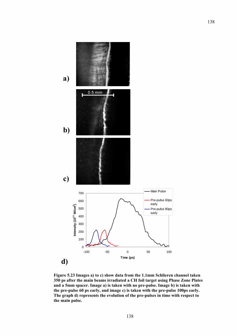
138
138
a)
b)
c)
d)
0
100
200
300
400
500
600
700
-100 -50 0 50 100
Time (ps)
Inte
nsity
(1011
W/c
m2 )
Main Pulse
Pre-pulse 60psearlyPre-pulse 80psearly
Figure 5.23 Images a) to c) show data from the 1.1mm Schlieren channel taken 350 ps after the main beams irradiated a CH foil target using Phase Zone Plates and a 5mm spacer. Image a) is taken with no pre-pulse. Image b) is taken with the pre-pulse 60 ps early, and image c) is taken with the pre-pulse 100ps early. The graph d) represents the evolution of the pre-pulses in time with respect to the main pulse.
139
139
5.5.3 Discussion
The success of this technique depends critically on the timing of the pre-pulse relative
to the main pulse as can be clearly seen in Figure 5.23. When the pre-pulse arrives
inside the envelope of the main pulse, or when the pre-pulse is not spatially filtered, the
identified PZP imprinted structure persists in the plasma. When the pre-pulse arrives
prior to the main pulse but has not ablated the target fully before the main pulse, then a
reduction of imprinted structure is observed. This would be consistent with a degree of
thermal smoothing, where the pressure modulations are significantly reduced during
transport from the absorption region to the ablation front. However, if the pre-pulse
arrives sufficiently early and completely ablates the foil prior to the main pulse, no
imprinting is observed at the sensitivity of our diagnostics. The upper limit on the
timing window for the pre-pulse is set by the plasma expanding to below critical
density.
5.6 Conclusions
An investigation into the production of plasma from 100nm scale thickness targets
using direct drive laser irradiation has been presented. The effects of target surface
structure and laser focus non-uniformity on the uniformity of the plasma have been
studied and characteristic scale length electron density features in the plasma have been
identified. Electron density profiles for various times in the evolution of the plasma
have been measured using an interferometer. Abel inversion of this data has shown
good agreement with one dimensional simulations and analytical models of the plasma
expansion. Measured leading edge expansion velocities are also in agreement with the
simulations. The ability of a spatially filtered pre-pulse to reduce the imprinted laser
focal spot structure has been demonstrated.
140
140
6 Chapter 6 - Colliding magnetised foils
6.1 Introduction
In this chapter, I will describe the experiments and results of a study aimed at producing
a laboratory collisionless shock. As outlined in Chapter 2, the formation of a
collisionless shock depends upon producing a suitable magnetised plasma and
interacting this plasma in a collisionless system. The approach is to take two similar
plasmas in an opposing geometry and allow them to flow together. The flow velocities,
density and ionisation state are chosen such that there are few collisions between the
counter-propagating plasmas. The role of the magnetic field is to introduce new scale
lengths to the system, which should be smaller than the ion-ion binary collision mean
free path. In addition, if the new scale lengths, or Larmor radii, are smaller than the size
of the system the dynamics of the counter-flowing plasmas are expected to be altered.
Scaling the system to a SNR as discussed in Chapter 2 requires a β of ~400. On
achieving such scaling, physics similar to that of a SNR is expected to be reproduced in
the laboratory.
Of considerable uncertainty, and interest, is the effect of an external magnetic field on
the experimentally created plasma. Experimental results presented here imply a
magnetic field of 7.5T, β of ~3000, does not effect the dynamics of an exploding foil.
Yet in a counter-propagating geometry the interaction between two plasmas is affected
by the presence of the external magnetic field. Details of the interaction between the
plasma and magnetic field are unknown, for example whether the magnetic field
penetrates the plasma.
6.2 Production of a magnetic field
The use of an external magnetic field in our experiments introduces several technical
challenges. From the scaling arguments for the experiment to be relevant to a 100 year
old SNR with the anticipated plasma conditions, the field strength needs to be
approximately 20T. To prevent effects of magnetic field variation on the plasma, as
documented in section 2.2.2, the generated field needs to be spatially and temporally
uniform over the extent of the plasma (1mm3) and duration of the experiment (~1ns). In

141
141
addition, the direction of the field should be perpendicular to the direction of the plasma
expansion.
The method used to generate the field must be compatible with the experimental
geometry required to produce two thin foil plasmas as described in Chapter 5. The
magnitude of the magnetic field should also be controllable to enable investigations of
the effect of magnetic field strength on the interaction. Two methods for magnetic field
generation have been investigated, 1) the use of a laser driven Helmholtz coil target and
2) a traditional pulsed power electromagnet.
6.2.1 Helmholtz coil laser target
Producing a multi-tesla, uniform magnetic field, synchronised with a laser-plasma
experiment can be achieved using a laser beam to generate a source of hot electrons,
which is used to drive an intense current. If the current flows in a loop, a magnetic field
is created. The methodology described here is based around the pioneering work of
Daido et al151,152, which was performed using a 10µm wavelength CO2 laser. The
essence of the method is outlined in Figure 6.1.
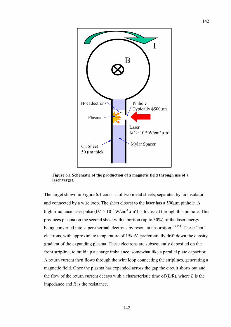
142
142
e-
I
B
LaserIλ2 > 1016 W/cm2 µm2
PinholeTypically φ500µm
Mylar SpacerCu Sheet50 µm thick
Plasma
Hot Electrons
Figure 6.1 Schematic of the production of a magnetic field through use of a laser target.
The target shown in Figure 6.1 consists of two metal sheets, separated by an insulator
and connected by a wire loop. The sheet closest to the laser has a 500µm pinhole. A
high irradiance laser pulse (Iλ2 > 1016 W/cm2 µm2) is focussed through this pinhole. This
produces plasma on the second sheet with a portion (up to 30%) of the laser energy
being converted into super-thermal electrons by resonant absorption153,154. These ‘hot’
electrons, with approximate temperature of 15keV, preferentially drift down the density
gradient of the expanding plasma. These electrons are subsequently deposited on the
front stripline, to build up a charge imbalance, somewhat like a parallel plate capacitor.
A return current then flows through the wire loop connecting the striplines, generating a
magnetic field. Once the plasma has expanded across the gap the circuit shorts out and
the flow of the return current decays with a characteristic time of (L/R), where L is the
impedance and R is the resistance.
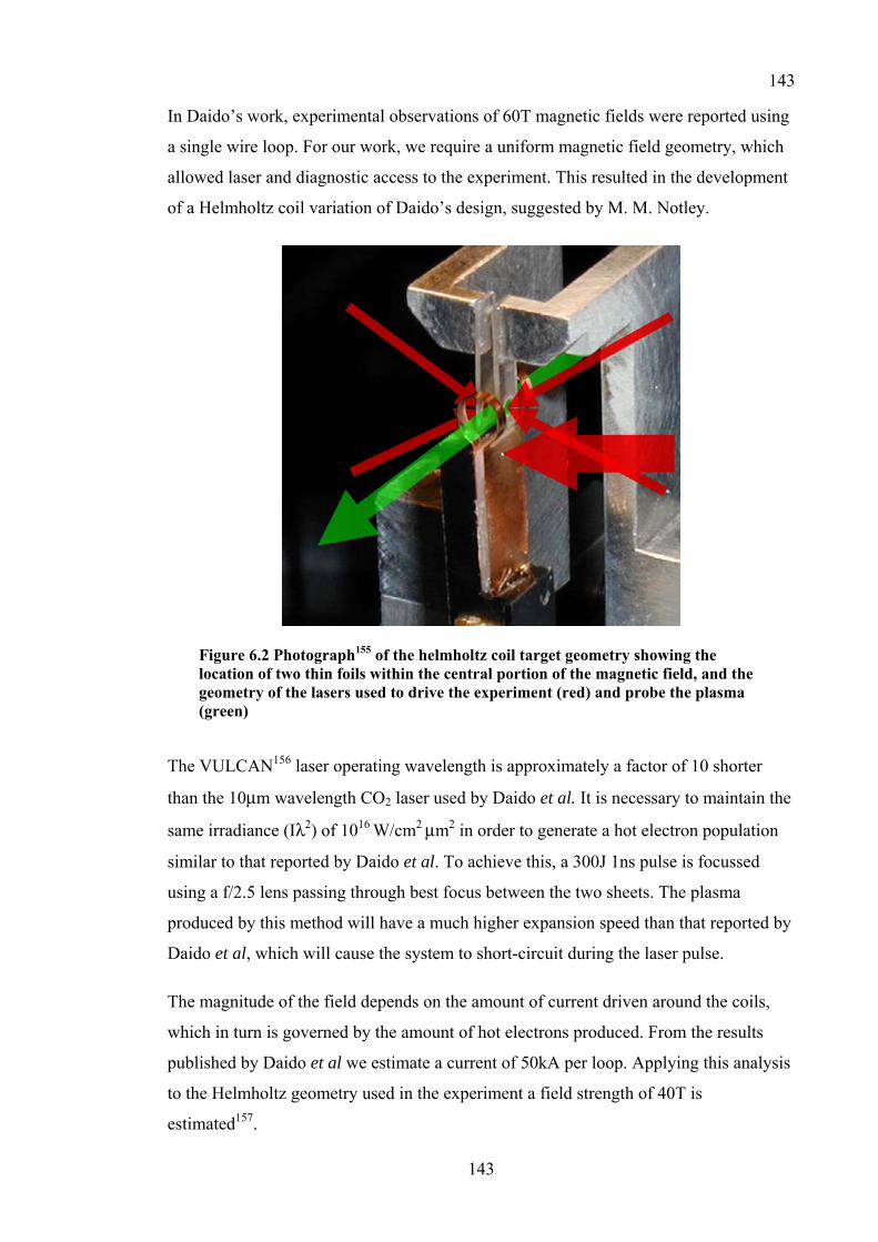
143
143
In Daido’s work, experimental observations of 60T magnetic fields were reported using
a single wire loop. For our work, we require a uniform magnetic field geometry, which
allowed laser and diagnostic access to the experiment. This resulted in the development
of a Helmholtz coil variation of Daido’s design, suggested by M. M. Notley.
Figure 6.2 Photograph155 of the helmholtz coil target geometry showing the location of two thin foils within the central portion of the magnetic field, and the geometry of the lasers used to drive the experiment (red) and probe the plasma (green)
The VULCAN156 laser operating wavelength is approximately a factor of 10 shorter
than the 10µm wavelength CO2 laser used by Daido et al. It is necessary to maintain the
same irradiance (Iλ2) of 1016 W/cm2 µm2 in order to generate a hot electron population
similar to that reported by Daido et al. To achieve this, a 300J 1ns pulse is focussed
using a f/2.5 lens passing through best focus between the two sheets. The plasma
produced by this method will have a much higher expansion speed than that reported by
Daido et al, which will cause the system to short-circuit during the laser pulse.
The magnitude of the field depends on the amount of current driven around the coils,
which in turn is governed by the amount of hot electrons produced. From the results
published by Daido et al we estimate a current of 50kA per loop. Applying this analysis
to the Helmholtz geometry used in the experiment a field strength of 40T is
estimated157.
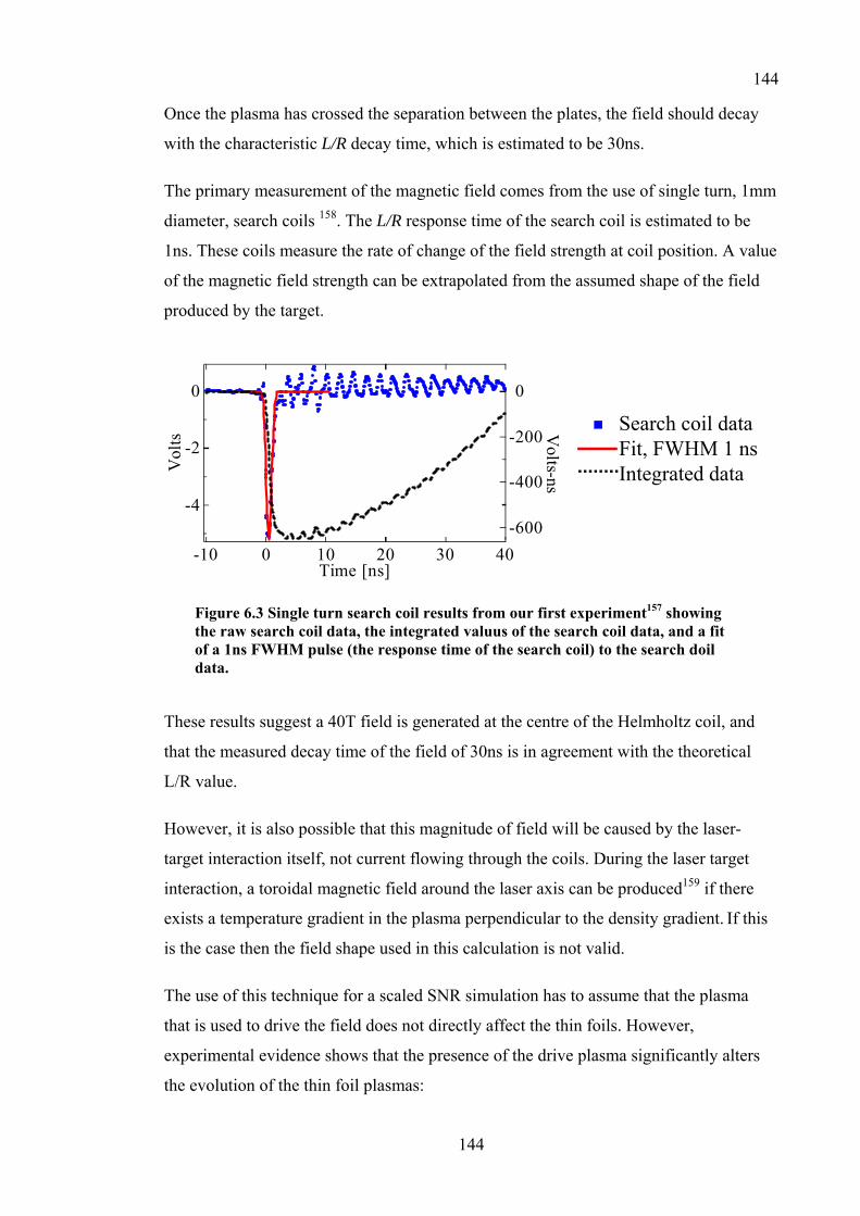
144
144
Once the plasma has crossed the separation between the plates, the field should decay
with the characteristic L/R decay time, which is estimated to be 30ns.
The primary measurement of the magnetic field comes from the use of single turn, 1mm
diameter, search coils 158. The L/R response time of the search coil is estimated to be
1ns. These coils measure the rate of change of the field strength at coil position. A value
of the magnetic field strength can be extrapolated from the assumed shape of the field
produced by the target.
-4
-2
0
Vol
ts
403020100-10Time [ns]
-600
-400
-200
0
Volts-ns
Search coil dataFit, FWHM 1 nsIntegrated data
Figure 6.3 Single turn search coil results from our first experiment157 showing the raw search coil data, the integrated valuus of the search coil data, and a fit of a 1ns FWHM pulse (the response time of the search coil) to the search doil data.
These results suggest a 40T field is generated at the centre of the Helmholtz coil, and
that the measured decay time of the field of 30ns is in agreement with the theoretical
L/R value.
However, it is also possible that this magnitude of field will be caused by the laser-
target interaction itself, not current flowing through the coils. During the laser target
interaction, a toroidal magnetic field around the laser axis can be produced159 if there
exists a temperature gradient in the plasma perpendicular to the density gradient. If this
is the case then the field shape used in this calculation is not valid.
The use of this technique for a scaled SNR simulation has to assume that the plasma
that is used to drive the field does not directly affect the thin foils. However,
experimental evidence shows that the presence of the drive plasma significantly alters
the evolution of the thin foil plasmas:
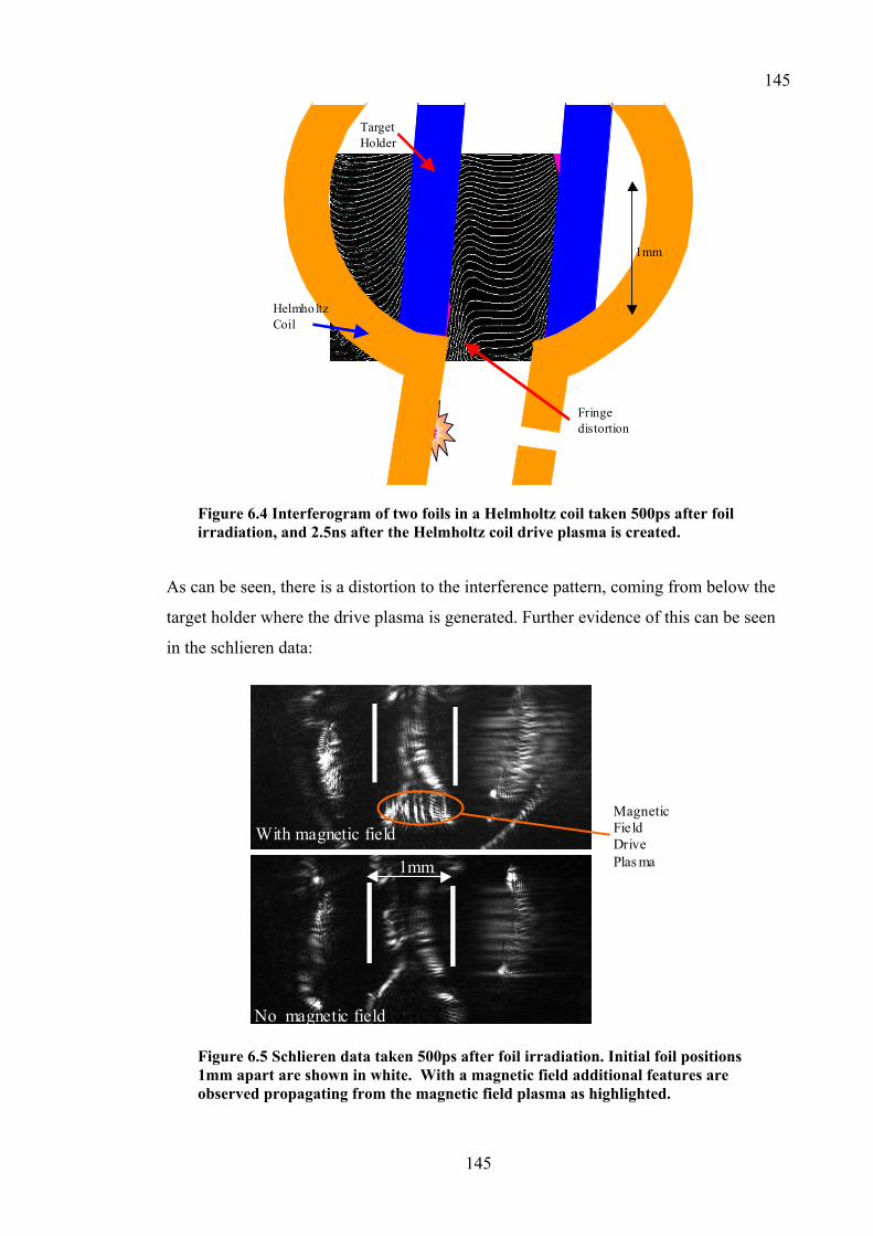
145
145
TargetHolder
HelmholtzCoil
1mm
Fringedistortion
Figure 6.4 Interferogram of two foils in a Helmholtz coil taken 500ps after foil irradiation, and 2.5ns after the Helmholtz coil drive plasma is created.
As can be seen, there is a distortion to the interference pattern, coming from below the
target holder where the drive plasma is generated. Further evidence of this can be seen
in the schlieren data:
0514
0516
With magnetic field
No magnetic field
MagneticFieldDrivePlas ma1mm
Figure 6.5 Schlieren data taken 500ps after foil irradiation. Initial foil positions 1mm apart are shown in white. With a magnetic field additional features are observed propagating from the magnetic field plasma as highlighted.
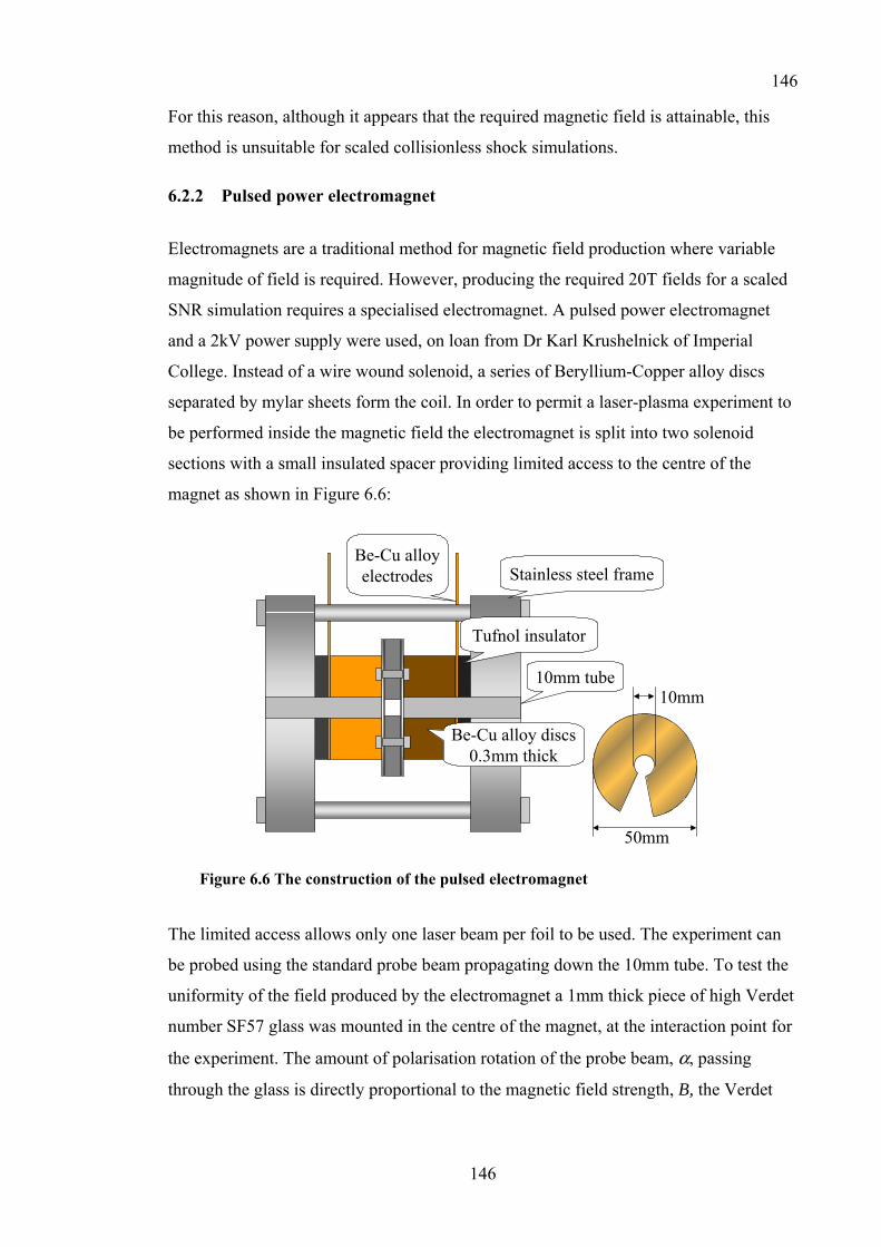
146
146
For this reason, although it appears that the required magnetic field is attainable, this
method is unsuitable for scaled collisionless shock simulations.
6.2.2 Pulsed power electromagnet
Electromagnets are a traditional method for magnetic field production where variable
magnitude of field is required. However, producing the required 20T fields for a scaled
SNR simulation requires a specialised electromagnet. A pulsed power electromagnet
and a 2kV power supply were used, on loan from Dr Karl Krushelnick of Imperial
College. Instead of a wire wound solenoid, a series of Beryllium-Copper alloy discs
separated by mylar sheets form the coil. In order to permit a laser-plasma experiment to
be performed inside the magnetic field the electromagnet is split into two solenoid
sections with a small insulated spacer providing limited access to the centre of the
magnet as shown in Figure 6.6:
Stainless steel frameBe-Cu alloyelectrodes
10mm tube
Tufnol insulator
Be-Cu alloy discs0.3mm thick
50mm
10mm
Figure 6.6 The construction of the pulsed electromagnet
The limited access allows only one laser beam per foil to be used. The experiment can
be probed using the standard probe beam propagating down the 10mm tube. To test the
uniformity of the field produced by the electromagnet a 1mm thick piece of high Verdet
number SF57 glass was mounted in the centre of the magnet, at the interaction point for
the experiment. The amount of polarisation rotation of the probe beam, α, passing
through the glass is directly proportional to the magnetic field strength, B, the Verdet

147
147
number and thickness of the glass. For SF57 the Verdet number is 1900°/T/m at 530nm.
The rotation was recorded by the polarimeter described in Chapter 4.
5mm
0 20 30 40 50 60 90
Figure 6.7 Polarogram of a glass slide inside the pulsed electromagnet, with the polarisation angle (in degrees) of each pixel represented by it’s colour as shown in the scale.
As can be seen from the data, the variation of the magnetic field over the surface of the
glass is negligible, whereas there is a 9° rotation with respect to the background. This
implies a 7.5T field would be generated from a 1.6kV pulse, the safe continuous
operating level of the magnet.
The temporal variation of the magnetic field was measured using a search coil mounted
in the centre of the magnet, and a Rogowski coil160 mounted around the power supply
cables. The integrated search coil signal provides a measurement of the magnetic field
strength, whereas the Rogowski coil diagnostic measures the amount of current flowing
into the magnet. As it is not possible to place a search coil in the magnet and explode
thin foils at the same time, calibrating the Rogowski coil to the search coil allows a
repetitive measurement of the magnetic field to be made.
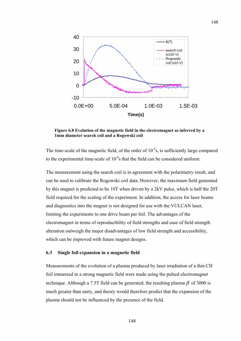
148
148
-10
0
10
20
30
40
0.0E+00 5.0E-04 1.0E-03 1.5E-03Time(s)
B(T)
search coil(x100 V)Rogowskicoil (x10 V)
Figure 6.8 Evolution of the magnetic field in the electromagnet as inferred by a 1mm diameter search coil and a Rogowski coil
The time-scale of the magnetic field, of the order of 10-4s, is sufficiently large compared
to the experimental time-scale of 10-9s that the field can be considered uniform.
The measurement using the search coil is in agreement with the polarimetry result, and
can be used to calibrate the Rogowski coil data. However, the maximum field generated
by this magnet is predicted to be 10T when driven by a 2kV pulse, which is half the 20T
field required for the scaling of the experiment. In addition, the access for laser beams
and diagnostics into the magnet is not designed for use with the VULCAN laser,
limiting the experiments to one drive beam per foil. The advantages of the
electromagnet in terms of reproducibility of field strengths and ease of field strength
alteration outweigh the major disadvantages of low field strength and accessibility,
which can be improved with future magnet designs.
6.3 Single foil expansion in a magnetic field
Measurements of the evolution of a plasma produced by laser irradiation of a thin CH
foil immersed in a strong magnetic field were made using the pulsed electromagnet
technique. Although a 7.5T field can be generated, the resulting plasma β of 3000 is
much greater than unity, and theory would therefore predict that the expansion of the
plasma should not be influenced by the presence of the field.

149
149
The experimental configuration is dictated by the use of a pulsed electromagnet to
generate the required magnetic field. Due to the limited access to the target position
only one laser beam can be used to irradiate the foil. To avoid possible issues with
surface currents being induced on the target holders the foils are mounted on Mylar
mounts and suspended from above the magnet on a Mylar rod.
The experimental arrangement is described in Figure 6.9:
Probe beam
∅108mm f/10 lensPZP,RPP or defocused∅1mm Spot
Imaging system
80ps 1054nm~3x10¹³ W/cm2
Optical probediagnostics
100nm thick foil target∅1.2mm
VacuumChamber
Electromagnet
~7.5T Magnetic field
Figure 6.9 Experimental chamber arrangement for magnetised single foil experiments. Note that only one beam per foil can be used due to the use of the electromagnet.
The electromagnet was used with a 1.6kV pulse triggered 300ms earlier than the
irradiating lasers to generate a 7.5T field around the target position to coincide with the
target irradiation.
The following measurements were made during the third experiment, with the
associated diagnostics and probe capabilities as described in Chapters 3 and 4
respectively. To ensure that the evolution of the plasma is not affected by the presence
of the field interferograms were taken after 750ps as shown in Figure 6.10:

150
150
a)
1.5mm
b)
1.5 mm
Figure 6.10 Interferograms taken 750ps after target irradiation with a) a 7.5T field and b) no magnetic field applied
The corresponding laser energies of 39J with magnetic field in a) and 42J without field
in b) are sufficiently close that the expansion should be nearly identical for both CH
foils. The electron density data is extracted from the interferograms using the
methodology described in section 4.2.4 to produce the Abel inverted electron densities
shown in Figure 6.11. Unfortunately, the thickness of the Mylar holder masks most of
the expansion of the foil towards the laser.
1.00E+17
1.00E+18
1.00E+19
-1.00E-01 -5.00E-02 0.00E+00 5.00E-02 1.00E-01
Distance (cm)
Elec
tron
Den
sity
(cm
-3)
0T Data7.5T Data
Figure 6.11 Abel inverted thin CH foil electron density profiles taken after 750ps
Laser Laser
Laser

151
151
The expansion of the plasmas away from the laser for both the magnetised and non
magnetised data shows a similar expansion profile, implying that the magnetic field
does not appear to affect the hydrodynamics of the expansion.
In interpreting the experimental results presented here, there lies one essential
unanswered issue. The fundamental problem is the penetration of the magnetic field into
the plasma. Here I will address this by examining the consequences of the field
penetrating the plasma and the field being excluded from the plasma on the
experimental results I have presented.
For the case of a single foil immersed in the magnetic field, if we assume that the
magnetic field penetrates the plasma, we have already stated that the plasma β is
sufficiently high that the expansion should not be affected by the presence of the field.
If we now assume the magnetic field is excluded from the plasma, the expansion of a
cylindrical plasma of radius r, would be halted161 after a distance LB, when the pressure
of the excluded magnetic field is equal to the initial pressure of the plasma:
220
rBE
LB = [6.1]
Where E0 is the energy of the plasma and B is the magnetic field. If the value of E0 is
approximately 1J, calculated from the kinetic energy of the expanding plasma for our
experiment, the value of LB is 5cm, much larger than the 0.5mm expansion. From this, it
would seem that both treatments show that the expansion up to the times observed
should be independent of the magnetic field. This simple analysis is supported by our
results.
6.4 Counter propagating exploding foil plasmas
The evolution of two counter propagating thin foil plasmas has been studied during all
three of our experiments, using both CH and Al foils. The foils are mounted faces
parallel, separated by 1mm and irradiated by one or two beams from VULCAN as
shown in Figure 6.12:
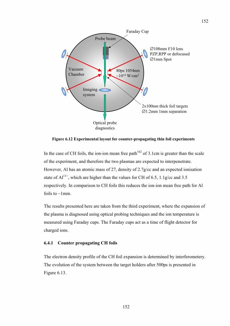
152
152
Probe beam
∅108mm f/10 lensPZP,RPP or defocused∅1mm Spot
Imaging system
80ps 1054nm~1014 W/cm2
Faraday Cup
Optical probediagnostics
2x100nm thick foil targets∅1.2mm 1mm separation
VacuumChamber
Figure 6.12 Experimental layout for counter-propagating thin foil experiments
In the case of CH foils, the ion-ion mean free path162 of 3.1cm is greater than the scale
of the experiment, and therefore the two plasmas are expected to interpenetrate.
However, Al has an atomic mass of 27, density of 2.7g/cc and an expected ionisation
state of Al11+, which are higher than the values for CH of 6.5, 1.1g/cc and 3.5
respectively. In comparison to CH foils this reduces the ion-ion mean free path for Al
foils to ~1mm.
The results presented here are taken from the third experiment, where the expansion of
the plasma is diagnosed using optical probing techniques and the ion temperature is
measured using Faraday cups. The Faraday cups act as a time of flight detector for
charged ions.
6.4.1 Counter propagating CH foils
The electron density profile of the CH foil expansion is determined by interferometery.
The evolution of the system between the target holders after 500ps is presented in
Figure 6.13.
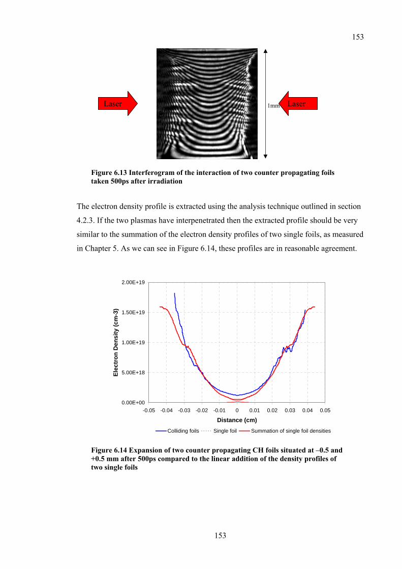
153
153
1mm
Figure 6.13 Interferogram of the interaction of two counter propagating foils taken 500ps after irradiation
The electron density profile is extracted using the analysis technique outlined in section
4.2.3. If the two plasmas have interpenetrated then the extracted profile should be very
similar to the summation of the electron density profiles of two single foils, as measured
in Chapter 5. As we can see in Figure 6.14, these profiles are in reasonable agreement.
0.00E+00
5.00E+18
1.00E+19
1.50E+19
2.00E+19
-0.05 -0.04 -0.03 -0.02 -0.01 0 0.01 0.02 0.03 0.04 0.05
Distance (cm)
Elec
tron
Den
sity
(cm
-3)
Colliding foils Single foil Summation of single foil densities
Figure 6.14 Expansion of two counter propagating CH foils situated at –0.5 and +0.5 mm after 500ps compared to the linear addition of the density profiles of two single foils
Laser Laser
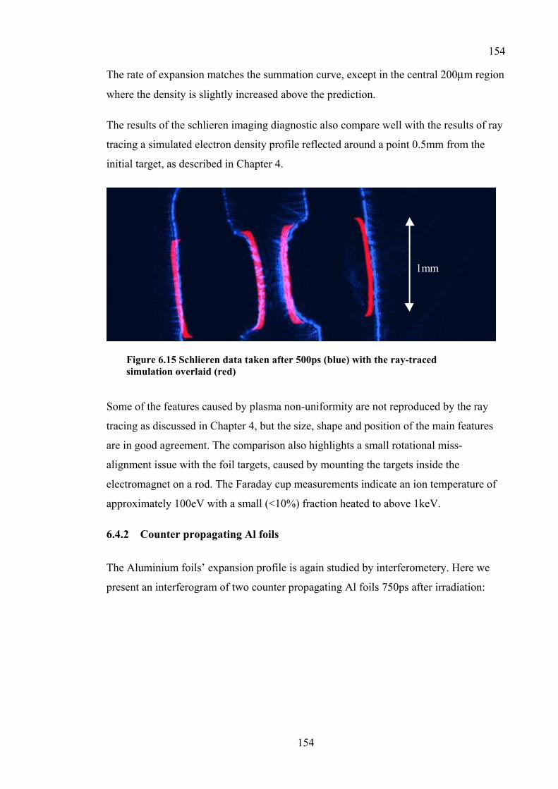
154
154
The rate of expansion matches the summation curve, except in the central 200µm region
where the density is slightly increased above the prediction.
The results of the schlieren imaging diagnostic also compare well with the results of ray
tracing a simulated electron density profile reflected around a point 0.5mm from the
initial target, as described in Chapter 4.
1mm
Figure 6.15 Schlieren data taken after 500ps (blue) with the ray-traced simulation overlaid (red)
Some of the features caused by plasma non-uniformity are not reproduced by the ray
tracing as discussed in Chapter 4, but the size, shape and position of the main features
are in good agreement. The comparison also highlights a small rotational miss-
alignment issue with the foil targets, caused by mounting the targets inside the
electromagnet on a rod. The Faraday cup measurements indicate an ion temperature of
approximately 100eV with a small (<10%) fraction heated to above 1keV.
6.4.2 Counter propagating Al foils
The Aluminium foils’ expansion profile is again studied by interferometery. Here we
present an interferogram of two counter propagating Al foils 750ps after irradiation:
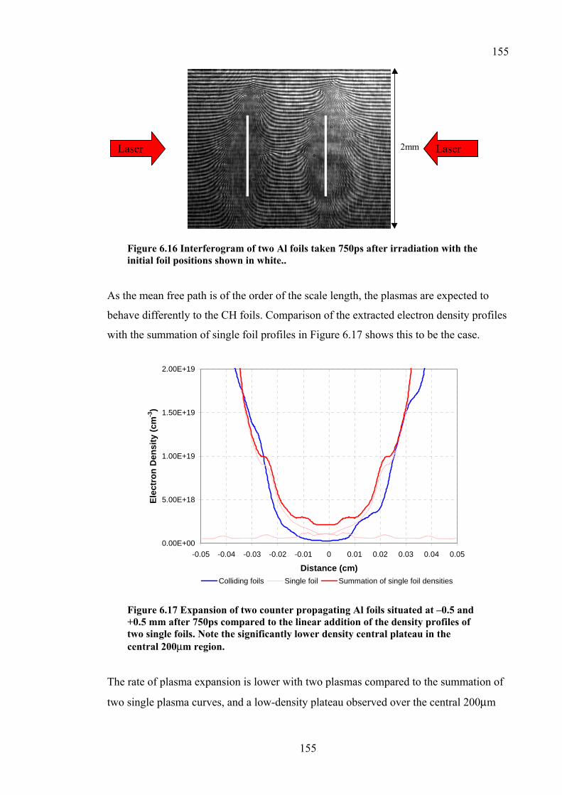
155
155
2mm
Figure 6.16 Interferogram of two Al foils taken 750ps after irradiation with the initial foil positions shown in white..
As the mean free path is of the order of the scale length, the plasmas are expected to
behave differently to the CH foils. Comparison of the extracted electron density profiles
with the summation of single foil profiles in Figure 6.17 shows this to be the case.
0.00E+00
5.00E+18
1.00E+19
1.50E+19
2.00E+19
-0.05 -0.04 -0.03 -0.02 -0.01 0 0.01 0.02 0.03 0.04 0.05
Distance (cm)
Elec
tron
Den
sity
(cm
-3)
Colliding foils Single foil Summation of single foil densities
Figure 6.17 Expansion of two counter propagating Al foils situated at –0.5 and +0.5 mm after 750ps compared to the linear addition of the density profiles of two single foils. Note the significantly lower density central plateau in the central 200µm region.
The rate of plasma expansion is lower with two plasmas compared to the summation of
two single plasma curves, and a low-density plateau observed over the central 200µm
Laser Laser
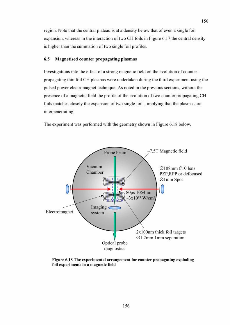
156
156
region. Note that the central plateau is at a density below that of even a single foil
expansion, whereas in the interaction of two CH foils in Figure 6.17 the central density
is higher than the summation of two single foil profiles.
6.5 Magnetised counter propagating plasmas
Investigations into the effect of a strong magnetic field on the evolution of counter-
propagating thin foil CH plasmas were undertaken during the third experiment using the
pulsed power electromagnet technique. As noted in the previous sections, without the
presence of a magnetic field the profile of the evolution of two counter propagating CH
foils matches closely the expansion of two single foils, implying that the plasmas are
interpenetrating.
The experiment was performed with the geometry shown in Figure 6.18 below.
Probe beam
∅108mm f/10 lensPZP,RPP or defocused∅1mm Spot
Imaging system
80ps 1054nm~3x10¹³ W/cm2
Optical probediagnostics
2x100nm thick foil targets∅1.2mm 1mm separation
VacuumChamber
Electromagnet
~7.5T Magnetic field
Figure 6.18 The experimental arrangement for counter propagating exploding foil experiments in a magnetic field
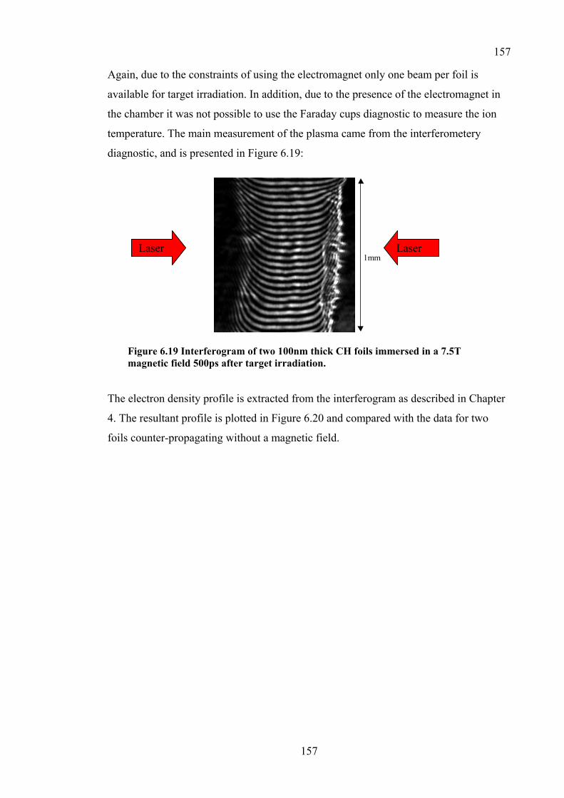
157
157
Again, due to the constraints of using the electromagnet only one beam per foil is
available for target irradiation. In addition, due to the presence of the electromagnet in
the chamber it was not possible to use the Faraday cups diagnostic to measure the ion
temperature. The main measurement of the plasma came from the interferometery
diagnostic, and is presented in Figure 6.19:
1mm
Figure 6.19 Interferogram of two 100nm thick CH foils immersed in a 7.5T magnetic field 500ps after target irradiation.
The electron density profile is extracted from the interferogram as described in Chapter
4. The resultant profile is plotted in Figure 6.20 and compared with the data for two
foils counter-propagating without a magnetic field.
Laser Laser

158
158
0.00E+00
5.00E+18
1.00E+19
1.50E+19
2.00E+19
-0.05 -0.04 -0.03 -0.02 -0.01 0 0.01 0.02 0.03 0.04 0.05
Distance (cm)
Elec
tron
Den
sity
(cm
-3)
0T Colliding foils 7.5T Colliding foils
Figure 6.20 Comparison of magnetised and non-magnetised colliding foil data after 500ps with initial foil positions situated at –0.5 and +0.5 mm. Note the similarity between this graph and Figure 6.17.
As can be seen from this graph, the expansion of the plasma appears to be retarded
compared to the non-magnetised case. Also there is a central 300µm wide low-density
plateau, reminiscent of the feature observed in the Al foil expansion in Figure 6.18. The
data also contains an unexpected central feature, as shown in Figure 6.21:
1mm
Figure 6.21 Interferometry reference channel image, showing the presence of a central feature between the two foils.
This feature is also observed, but with less clarity on other diagnostics. Similar type
structures were observed at 450ps and 550ps, although with less clarity than this shot. It
is also very interesting to note that a similar feature is observed in the data from a
Helmholtz coil driven experiment, as shown in Figure 6.22:
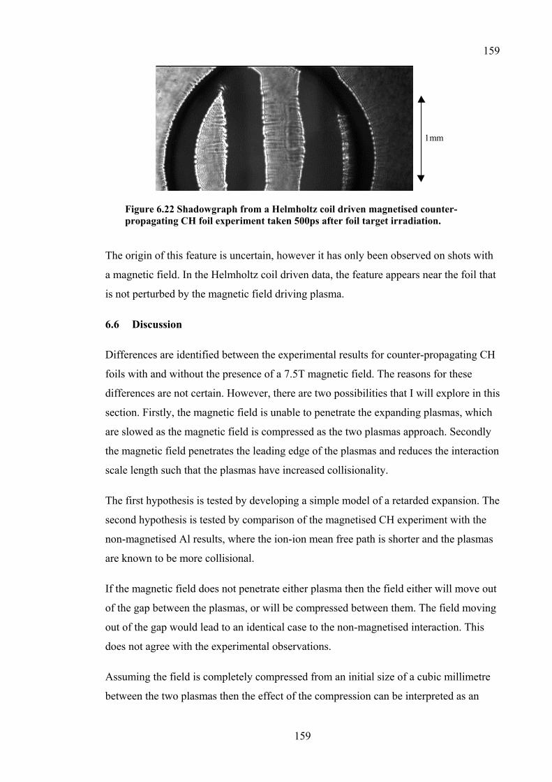
159
159
1mm
Figure 6.22 Shadowgraph from a Helmholtz coil driven magnetised counter-propagating CH foil experiment taken 500ps after foil target irradiation.
The origin of this feature is uncertain, however it has only been observed on shots with
a magnetic field. In the Helmholtz coil driven data, the feature appears near the foil that
is not perturbed by the magnetic field driving plasma.
6.6 Discussion
Differences are identified between the experimental results for counter-propagating CH
foils with and without the presence of a 7.5T magnetic field. The reasons for these
differences are not certain. However, there are two possibilities that I will explore in this
section. Firstly, the magnetic field is unable to penetrate the expanding plasmas, which
are slowed as the magnetic field is compressed as the two plasmas approach. Secondly
the magnetic field penetrates the leading edge of the plasmas and reduces the interaction
scale length such that the plasmas have increased collisionality.
The first hypothesis is tested by developing a simple model of a retarded expansion. The
second hypothesis is tested by comparison of the magnetised CH experiment with the
non-magnetised Al results, where the ion-ion mean free path is shorter and the plasmas
are known to be more collisional.
If the magnetic field does not penetrate either plasma then the field either will move out
of the gap between the plasmas, or will be compressed between them. The field moving
out of the gap would lead to an identical case to the non-magnetised interaction. This
does not agree with the experimental observations.
Assuming the field is completely compressed from an initial size of a cubic millimetre
between the two plasmas then the effect of the compression can be interpreted as an
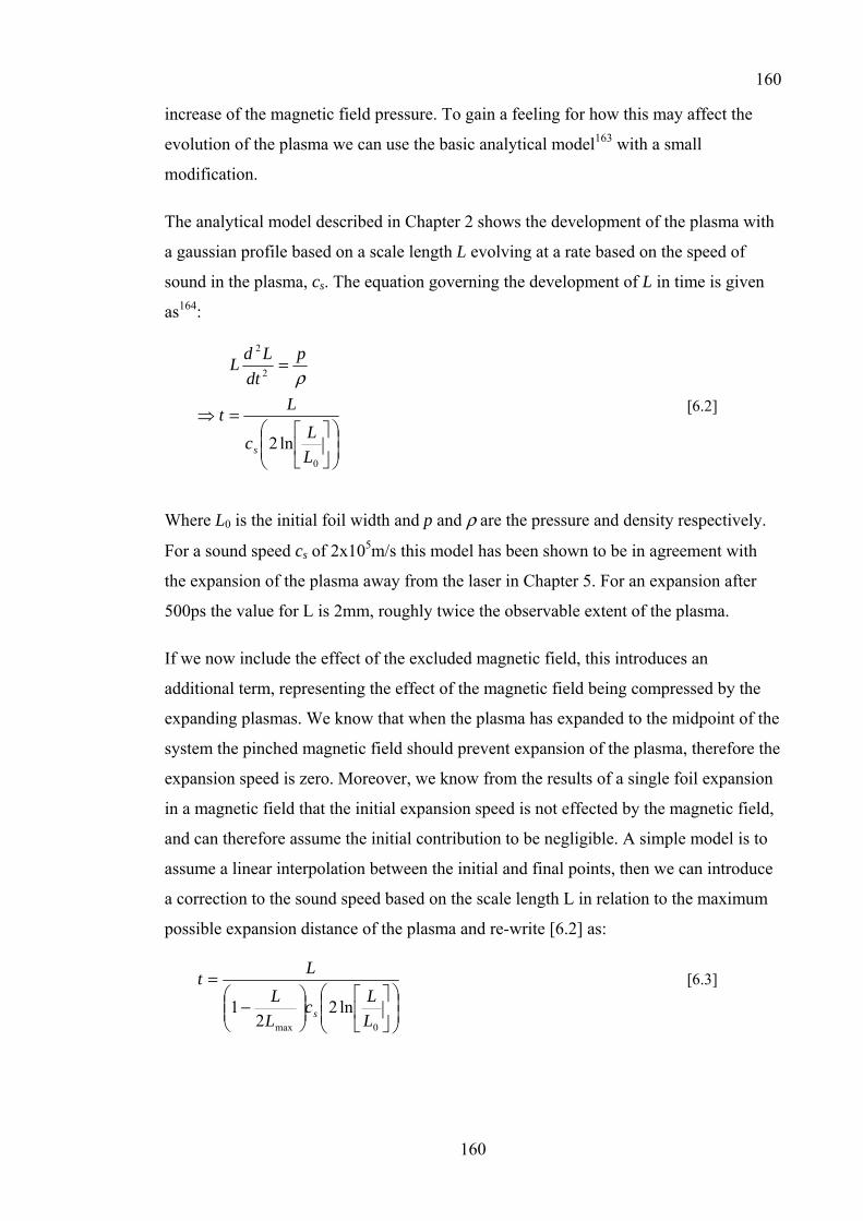
160
160
increase of the magnetic field pressure. To gain a feeling for how this may affect the
evolution of the plasma we can use the basic analytical model163 with a small
modification.
The analytical model described in Chapter 2 shows the development of the plasma with
a gaussian profile based on a scale length L evolving at a rate based on the speed of
sound in the plasma, cs. The equation governing the development of L in time is given
as164:
⎟⎟⎠
⎞⎜⎜⎝
⎛⎥⎦
⎤⎢⎣
⎡=⇒
=
0
2
2
ln2LLc
Lt
pdt
LdL
s
ρ [6.2]
Where L0 is the initial foil width and p and ρ are the pressure and density respectively.
For a sound speed cs of 2x10⁵m/s this model has been shown to be in agreement with
the expansion of the plasma away from the laser in Chapter 5. For an expansion after
500ps the value for L is 2mm, roughly twice the observable extent of the plasma.
If we now include the effect of the excluded magnetic field, this introduces an
additional term, representing the effect of the magnetic field being compressed by the
expanding plasmas. We know that when the plasma has expanded to the midpoint of the
system the pinched magnetic field should prevent expansion of the plasma, therefore the
expansion speed is zero. Moreover, we know from the results of a single foil expansion
in a magnetic field that the initial expansion speed is not effected by the magnetic field,
and can therefore assume the initial contribution to be negligible. A simple model is to
assume a linear interpolation between the initial and final points, then we can introduce
a correction to the sound speed based on the scale length L in relation to the maximum
possible expansion distance of the plasma and re-write [6.2] as:
⎟⎟⎠
⎞⎜⎜⎝
⎛⎥⎦
⎤⎢⎣
⎡⎟⎟⎠
⎞⎜⎜⎝
⎛−
=
0max
ln22
1LLc
LL
Lt
s
[6.3]
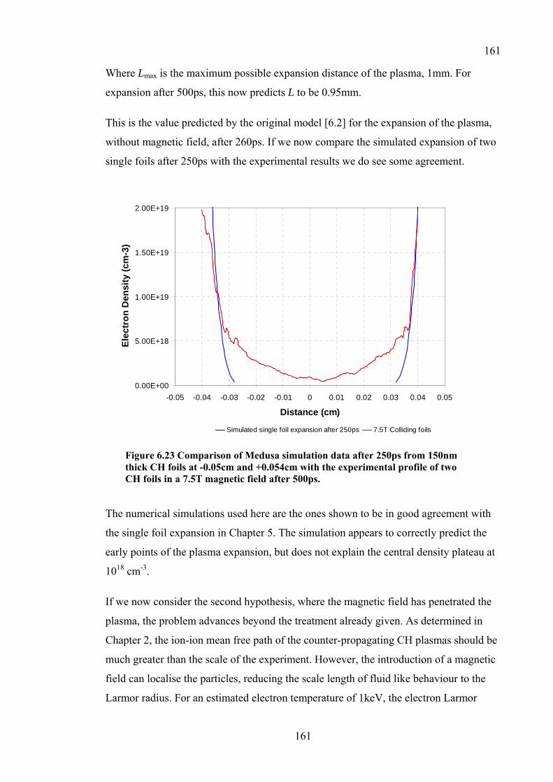
161
161
Where Lmax is the maximum possible expansion distance of the plasma, 1mm. For
expansion after 500ps, this now predicts L to be 0.95mm.
This is the value predicted by the original model [6.2] for the expansion of the plasma,
without magnetic field, after 260ps. If we now compare the simulated expansion of two
single foils after 250ps with the experimental results we do see some agreement.
0.00E+00
5.00E+18
1.00E+19
1.50E+19
2.00E+19
-0.05 -0.04 -0.03 -0.02 -0.01 0 0.01 0.02 0.03 0.04 0.05
Distance (cm)
Elec
tron
Den
sity
(cm
-3)
Simulated single foil expansion after 250ps 7.5T Colliding foils
Figure 6.23 Comparison of Medusa simulation data after 250ps from 150nm thick CH foils at -0.05cm and +0.054cm with the experimental profile of two CH foils in a 7.5T magnetic field after 500ps.
The numerical simulations used here are the ones shown to be in good agreement with
the single foil expansion in Chapter 5. The simulation appears to correctly predict the
early points of the plasma expansion, but does not explain the central density plateau at
1018 cm-3.
If we now consider the second hypothesis, where the magnetic field has penetrated the
plasma, the problem advances beyond the treatment already given. As determined in
Chapter 2, the ion-ion mean free path of the counter-propagating CH plasmas should be
much greater than the scale of the experiment. However, the introduction of a magnetic
field can localise the particles, reducing the scale length of fluid like behaviour to the
Larmor radius. For an estimated electron temperature of 1keV, the electron Larmor
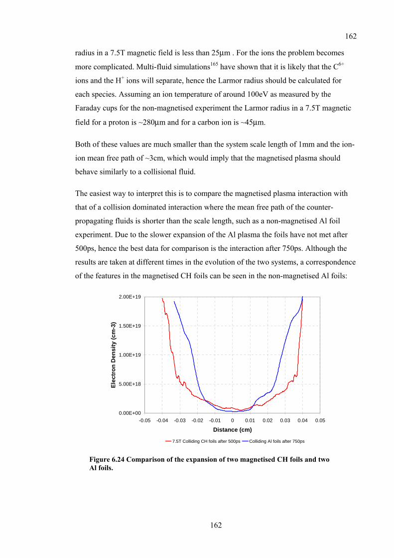
162
162
radius in a 7.5T magnetic field is less than 25µm . For the ions the problem becomes
more complicated. Multi-fluid simulations165 have shown that it is likely that the C6+
ions and the H+ ions will separate, hence the Larmor radius should be calculated for
each species. Assuming an ion temperature of around 100eV as measured by the
Faraday cups for the non-magnetised experiment the Larmor radius in a 7.5T magnetic
field for a proton is ~280µm and for a carbon ion is ~45µm.
Both of these values are much smaller than the system scale length of 1mm and the ion-
ion mean free path of ~3cm, which would imply that the magnetised plasma should
behave similarly to a collisional fluid.
The easiest way to interpret this is to compare the magnetised plasma interaction with
that of a collision dominated interaction where the mean free path of the counter-
propagating fluids is shorter than the scale length, such as a non-magnetised Al foil
experiment. Due to the slower expansion of the Al plasma the foils have not met after
500ps, hence the best data for comparison is the interaction after 750ps. Although the
results are taken at different times in the evolution of the two systems, a correspondence
of the features in the magnetised CH foils can be seen in the non-magnetised Al foils:
0.00E+00
5.00E+18
1.00E+19
1.50E+19
2.00E+19
-0.05 -0.04 -0.03 -0.02 -0.01 0 0.01 0.02 0.03 0.04 0.05
Distance (cm)
Elec
tron
Den
sity
(cm
-3)
7.5T Colliding CH foils after 500ps Colliding Al foils after 750ps
Figure 6.24 Comparison of the expansion of two magnetised CH foils and two Al foils.
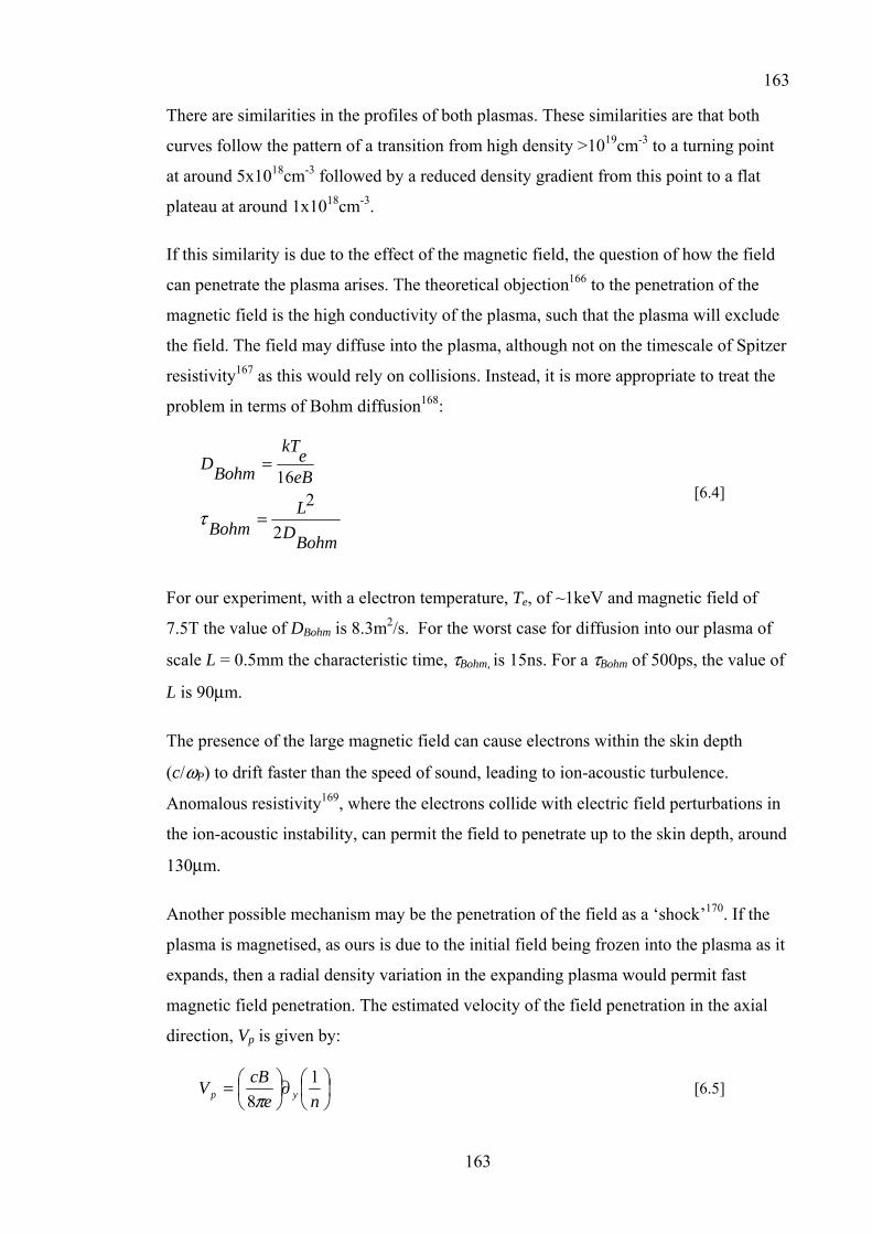
163
163
There are similarities in the profiles of both plasmas. These similarities are that both
curves follow the pattern of a transition from high density >1019cm-3 to a turning point
at around 5x1018cm-3 followed by a reduced density gradient from this point to a flat
plateau at around 1x1018cm-3.
If this similarity is due to the effect of the magnetic field, the question of how the field
can penetrate the plasma arises. The theoretical objection166 to the penetration of the
magnetic field is the high conductivity of the plasma, such that the plasma will exclude
the field. The field may diffuse into the plasma, although not on the timescale of Spitzer
resistivity167 as this would rely on collisions. Instead, it is more appropriate to treat the
problem in terms of Bohm diffusion168:
BohmDL
Bohm
eBekT
BohmD
2
216
=
=
τ [6.4]
For our experiment, with a electron temperature, Te, of ~1keV and magnetic field of
7.5T the value of DBohm is 8.3m2/s. For the worst case for diffusion into our plasma of
scale L = 0.5mm the characteristic time, τBohm, is 15ns. For a τBohm of 500ps, the value of
L is 90µm.
The presence of the large magnetic field can cause electrons within the skin depth
(c/ωP) to drift faster than the speed of sound, leading to ion-acoustic turbulence.
Anomalous resistivity169, where the electrons collide with electric field perturbations in
the ion-acoustic instability, can permit the field to penetrate up to the skin depth, around
130µm.
Another possible mechanism may be the penetration of the field as a ‘shock’170. If the
plasma is magnetised, as ours is due to the initial field being frozen into the plasma as it
expands, then a radial density variation in the expanding plasma would permit fast
magnetic field penetration. The estimated velocity of the field penetration in the axial
direction, Vp is given by:
⎟⎠⎞
⎜⎝⎛∂⎟
⎠⎞
⎜⎝⎛=
necBV yp
18π
[6.5]
164
164
Where ∂y(1/n) is the inverse of the radial density gradient. Although the expansion of
the foil is approximately one-dimensional, there is a radial component to the observed
electron density profiles, as shown in Figure 6.25.
1E+18
1E+19
1E+20
0 0.1 0.2 0.3 0.4 0.5 0.6
Radial distance (mm)
Mag
nitu
de o
f rad
ial e
lect
ron
dens
ity g
radi
ent (
cm-3
mm
-1)
Figure 6.25 Abel inverted radial density gradient profile at the midpoint of two counter propagating CH foils immersed in a 7.5T magnetic field.
For our experiment, taking a radial density gradient of around 1019cm-3mm-1 and a 7.5T
field, this gives a value for Vp of 5.5x107 cm/s. This rate of penetration is slower than
the observed plasma expansion speed of 1.55x108 cm/s. Hence, the field should
penetrate ~166µm the plasma. It is interesting to note that the penetration speed is faster
for lower variations in radial density, and therefore any significant radial non-uniformity
may prevent magnetic field penetration. It is also interesting to note that for the
designed experimental magnetic field strength of 20T the predicted velocity of field
penetration would be 1.46 x108 cm/s, approximately the expansion velocity.
All of these treatments show that the plasma regions involved in the initial phase of the
interaction between two counter-propagating CH foils may be magnetised.
6.7 Conclusions
The experiments described in this chapter were designed to demonstrate the
fundamental processes that underpin the formation of a collisionless shock.

165
165
This has been achieved by demonstrating that we are able to produce high β plasma
from thin foils, as the hydrodynamics of the foil expansion are not affected by the
magnetic field. We have then gone on to demonstrate that plasmas can be produced in a
counter propagating collision free system where the two plasmas interpenetrate.
I have also demonstrated the behaviour of a highly collisional interaction in the same
geometry, and proceeded show that this form of behaviour is akin to that exhibited by
high β plasmas in a counter propagating collision free system with the presence of an
external magnetic field.
I have also discussed whether this observed form of behaviour may also be explained by
the effects of magnetic field compression retarding the flow of the plasma. I conclude
that there is stronger experimental evidence to support the view of magnetic field
penetration, and that there are potential theoretical mechanisms to enable this to occur.
However, this awaits conclusive proof by measurement of the strength of the magnetic
field inside the plasmas, possibly through Faraday rotation or Zeeman splitting.
:
166
166
7 Chapter 7 - Conclusions
In drawing together the body of work presented in this thesis, this chapter provides a
summary of the work and it’s conclusions. In this context, I will discuss the possible
avenues for continuation of this research.
7.1 Conclusions
This thesis presents the beginning of an investigation into the interaction of two rapidly
expanding laser-produced plasmas immersed in a strong magnetic field. From the
outset, our aim has been to produce an experimental system that could be used for
scaled simulation studies appropriate to a 100 year old supernova remnant. The
simulation is a snapshot in time, which does not attempt to model the evolution of the
supernova remnant. This approach is different to that used elsewhere in simulating
young supernovae. Considerable progress towards this goal has been made through a
series of experiments performed using the VULCAN laser at the Rutherford – Appleton
Laboratory.
In Chapter 2 I have shown how a collisionless shock may be formed in a plasma. The
formation of a collisionless system, i.e. where the mean free path of the particles in the
plasma is much greater than the scale of the system, can be achieved in a low density,
low Z counter propagating system where the relative velocities of the plasmas involved
is high. If a magnetic field is present within the system it can introduce fluid like
behaviour by localising the particles in the plasma. The corresponding scale length for
this type of interaction is the Larmor radius of the particles. The further constraint is
that the Larmor radius is less than the system size.
I have also introduced the concept of scaling and shown that by numerical simulation an
experiment can be designed to be similar to a 100 year old supernova remnant by
matching a series of four key dimensionless constants between the two systems. Firstly,
the Euler number of the two systems must be similar, which requires that the system can
be described by the ideal fluid equations. Secondly, the plasma β must also be matched
to relate the effect of the magnetic field in both systems. Thirdly the system must
produce a strong shock, with a Mach number greater than 1. Finally, the system must be
167
167
collisionless, with the mean free path greater than the scale length of the system.
Experimental work has been undertaken to attempt to produce such an experiment.
The principle diagnostic used in this experimental work has been optical probing. An
optical probe providing simultaneous shadowgraphy, interferometery, Schlieren
imaging and polarimetry measurements was used. The development of optical probe
beam design for use in our experiments, along with a suitable imaging system tailored
to the requirements of particular experiments have been presented in chapter 3. The
employment of the utilised optical probe diagnostics has been investigated in chapter 4,
where I have demonstrated the theory behind the diagnostic measurements, and also the
development of techniques for analysing experimental data for interferometery,
Schlieren and polarimetry diagnostics.
The experimental scheme described in Chapter 5 is based upon the laser irradiation of
~100nm thick targets. Optical probe data is presented and shows the formation of a
rapidly expanding, low-density plasma using this technique. The plasma evolution was
found to be in good agreement with both analytical and numerical modelling of the
plasma expansion.
However, measurement illustrated that the plasma produced from such thin foil targets
is susceptible to non-uniformity. The source of the structure was found to be both target
surface structure and imprinting of the laser focal spot profile. To eliminate this, two
approaches were taken. Firstly, improvements were made to the targets through more
uniform film production and target holder developments. Secondly, the laser beam used
to explode the foils was smoothed. Experimentally observed imprinting into the plasma
of structure in the focus of the laser has been found to be limited by the use of a
spatially filtered pre-pulse. From this investigation, and implementing these techniques
it is possible to conclude that a smooth plasma can be created.
The experimental production of uniform thin foil plasma can be accurately designed to
meet scaling criteria through the numerical simulation methods used. In addition, the
behaviour of thin foil plasma has been characterised to an extent that enables
interpretation of thin foil interaction experiments.
In Chapter 6, the experimental use of thin foil plasma in a counter propagating geometry
was used to simulate a collisionless interraction. Measurements with and without a
168
168
magnetic field are compared. Generating the required magnetic field is difficult and two
separate methods of magnetic field production have been experimentally investigated,
the use of a laser-plasma driven Helmholtz coil target and a pulsed power
electromagnet. It was determined that the pulsed power electromagnet was the
preferential experimental solution, despite having a lower field strength generated than
required by the scaling criteria, as the mechanism for generating the field did not
interfere with performing an experiment within the field.
It was observed that the magnetic field did not effect the hydrodynamics of a single
foil’s expansion. In addition, the use of counter propagating CH foils produced a
collisionless system as the two plasmas interpenetrated in agreement with expectation
and confirmed by comparison with the summation of the density profiles of two
separate foils. The affect of a magnetic field on the interaction of two counter
propagating CH foil plasmas was to modify the system such that the observed behaviour
is similar to the interaction of two Al foils without a magnetic field.
The plasma parameters we have been able to produce are not in agreement with the
scaling conditions, and we have not produced a collisionless shock in the experiments
presented here. However, this is mainly due to technological constraints on the
production of a sufficiently strong magnetic field, which can be improved upon in
future experiments.
From this thesis, I can conclude that the presence of a suitable magnetic field could be
interpreted as introducing an effective collisionality to the collisionless system we have
created, producing fluid like behaviour. This is the cornerstone of collisionless shock
formation, and hopefully will lead to the lead to the production of a collisionless shock
with continued developments to the experimental technique.
7.2 Further Work
The experimental program of which the first three experiments are presented in this
thesis is ongoing. At the time of writing, another experiment in this series is underway
utilising an electromagnet designed and constructed within our research group. This
development should bring the parameters of the experiment closer to the designed
criteria for a scaled simulation, and possibly the formation of a collisionless shock.
169
169
There are still outstanding issues that need to be addressed within the current
experimental system. Probably the most fundamental of these is the evidence for
magnetic field penetration into the expanding plasma, which may be investigated
experimentally. A measurement of the strength of the magnetic field inside the plasmas
is required to conclusively determine the role of the magnetic field in the interaction.
This may be possible through Faraday rotation if the magnetic field strength is increased
and a more accurate polarimeter design can be constructed. Alternatively, it may be
possible to look for spectroscopic evidence of field penetration from a Zeeman splitting
diagnostic.
The degree of field penetration may also be investigated indirectly by studying the
proposed mechanisms by which field penetration may occur. For example, if the
proposed method of magnetic field penetration by a shock is to be tested, varying the
radial uniformity of the plasma through varying the focussing techniques used should
affect the rate of field penetration.
With sufficient diagnostic access through the new electromagnet the ion temperature
within the plasma may be measured, possibly by Thomson scattering, and possibly
temporally resolved. If this shows an increase in the ion temperature coinciding with the
interaction of the two plasmas, this would provide strong evidence for the start of shock
formation.
As the initial experimental design was constrained by the laser output of VULCAN it
may be possible in the future to take advantages of proposed upgrades to VULCAN or
use other facilities to produce larger scale length plasmas within a similar one-
dimensional geometry. This would decrease the required magnetic field strength to
localise the particles sufficiently for scaling, which is the current experimental
limitation.
If this experimental series enables us to form a collisionless shock, there is the very
interesting possibility of being able to study the ‘injection problem’ of particles being
accelerated to cosmic rays by collisionless shocks.
170
170
List of references
1 B. Remington et al, Science, 284,1488 (1999)
2 G. Collins et al, Physics of Plasmas, 5, 5, 1864, (1998)
3 J. Wark et al, Physics of Plasmas, 4, 5, 2004, (1997)
4 D. Ryutov et al, Ast. J, 518, 821-832, (2000)
5 D. D. Ryutov and B. A. Remington, Plasma Phys. Contr. Fusion, 44, B407, (2002)
6 S. Lebedev et al, Ast. J, 564,113-119, (2002)
7 S. Rose, Physics World, 54, Apr (1994)
8 K. Shigemori et al, Physical Review E, 62, 6, 8838, (2000)
9 D. R. Farley et al, Phys. Rev. Lett. , 83, 10, 1982, (1999)
10 R. Klein et al, Ast J. Supp 127, 379-383 (2000)
11 R. Dendy and J. Kirk, Plasma Phys. Contr. Fusion, 41, A427-A435, (1999)
12 T. J. M. Boyd and J. J. Sanderson, ‘The Physics of Plasmas’, Cambridge University
Press, (2003), Chapter 5.2
13 M. Brown et al. Ast. J. Lett, 577, L63-L66, (2002)
14 M. A. Malkov and P. H. Diamond, Physics of Plasmas, 8, 4, 2401, (2001)
15 A. R. Bell, Mon. Not. R. astr. Soc. 182, 147, (1978)
16 L. Drury, Adv. Space Res. 15, 8/9, 481-487, (1995)
17 Koyama et al, Nature, 378, 255, (1995)
18 G. P. Zank et al, Physics of Plasmas, 8, 10, 4560, (2001)
171
171
19 M. Scholer, H. Kucharek and K. J. Trattner, Adv. Space Res., 21, 4, 533, (1998)
20 R. Sagdeev and C.Kennel, Scientific Americam, 40, Apr (1991)
21 R. P. Drake, Physics of Plasmas, 7, 11, 4690, (2000)
22 B. H. Ripin et al, Laser Part Beams, 8, 183, (1990)
23 B. A. Remington, Physics of Plasmas, 7, 5, 1641, (2000)
24 H. Takabe et al, Plasma Phys. Contr. Fusion, 41, A75, (1999)
25 Y. P. Zakharov, ‘Collisionless Laboratory astrophysics with Lasers’.
26 R. P. Drake, J. Geophys Research, 104, A7, 14505 (1999)
27 R. P. Drake et al, Physics of Plasmas, 7, 5, 2142, (2000)
28 R. P. Drake et al, Astrophysical Journal Supplement Series, 127, 305, (2000)
29 J. Kane et al, Astrophysical Journal, 478, L75, (1997)
30 K. Shigemori et al, Astrophysical Journal, 533, L159, (2000)
31 C. F. McKee and B. T. Draine, Science, 252, 397, (1991)
32 R. I. Klein et al, Astrophysical Journal, 583, 245, (2003)
33 R. J. Taylor, D. R. Baker and H. Ikezi, Phys. Rev. Lett., 24, 5, 206, (1970)
34 D. W. Forslund and C. R. Shonk, Phys. Rev. Lett., 25, 25, 1699, (1970)
35 D. W. Koopman and D. A. Tidman, Phys. Rev. Lett., 18, 14, 533, (1967)
36 Dean et al, Phys. Rev. Lett., 27, 8, 487, (1971)
37 T. J. M. Boyd and J. J. Sanderson, ‘The Physics of Plasmas’, Cambridge University
Press, (2003), Chapter 6.5.1

172
172
38 T. P. Wright, Phys. Rev. Lett., 28, 5, 268, (1972)
39 Dean et al, Phys. Rev. Lett., 29, 9, 569, (1972)
40 A. Y. Cheung, R. R. Goforth and D. W. Koopman, Phys. Rev. Lett., 31, 7, 429,
(1973)
41 A. R. Bell et al, Physical Review A, 38, 3, 1363, (1988)
42 R. Decoste et al, Phys. Rev. Lett., 42, 25, 1673, (1979)
43 R. A. London and M. D. Rosen, Phys. Fluids, 29, 11, 3813, (1986)
44 P Helander, et al. CLF Annual Report 2000-2001, 58 (2001).
45 M. D. Rosen et al, Phys Rev Lett, 54, 2, 106 (1985)
46 E. A. McLean et al, Phys. Rev. Lett., 45, 15, 1246, (1980)
47 J. Grun et al, Phys. Rev. Lett., 66, 21, 2738, (1991)
48 A. Raven et al, Phys. Rev. Lett., 47,15, 1049, (1981)
49 R. R. Whitlock et al, Phys. Rev. Lett., 52, 10, 819, (1984)
50 J. Grun et al, Phys. Rev. Lett., 53, 14, 1352, (1984)
51 T. R. Boehly et al, J. of Applied Physics, 92, 3, 1212, (2002)
52 S. P. Obenschain et al, Phys. Rev. Lett., 46, 21, 1402, (1981)
53 J. H. Gardner and S. E. Bodner, Phys. Rev. Lett., 47, 16, 1137, (1981)
54 A. J. Cole et al, J. Phys. D., 15, 1689, (1982)
55 S. G. Glendinning et al, Phys. Rev. Lett., 80, 9, 1904, (1998)
56 J. Grun et al. Phys. Rev. Lett., 58, 25, 2672, (1987)
173
173
57 D. S. Montgomery et al, Physics of Plasmas, 3, 5, 1728, (1996)
58 P. T. Rumsby, J. W. M. Paul and M. M. Masoud, Plasma Physics, 16, 969, (1974)
59 Berger et al, Phys. Fluids. B., 3, 1, 3, (1991)
60 Bosch et al, Physics of Fluids, 4, 4, 979, (1992)
61 P.W. Rambo and J. Denavit, Physics of Plasmas, 1, 12, 4050, (1994)
62 O. Larroche, Phys. Fluids B., 5, 8, 2816, (1993)
63 P. W. Rambo and R. J. Procassini, Physics of Plasmas, 2, 8, 3130, (1995)
64 T. S. Perry et al, Astrophysical Journal Supplement Series, 127, 437, (2000)
65 O. Rancu et al. Phys. Rev. Lett., 75, 21, 3854, (1995)
66 C. Chenais-Popovics et al, Physics of Plasmas, 4, 1, 190, (1997)
67 F.F. Chen, ‘Introduction to Plasma Physics’, Plenum Press, (1974) p.3
68 T. M. O’Neil and P. V. Coroniti, Rev. Modern Phys., 71, 2, S404, (1999)
69 R.O. Dendy, ‘Plasma Physics: An Introductory Course’, Cambridge University Press,
(1993)
70 F.F. Chen, ‘Introduction to Plasma Physics’, Plenum Press, (1974)
71 T. J. M. Boyd and J. J. Sanderson, ‘The Physics of Plasmas’, Cambridge University
Press, (2003)
72 A.R. Choudhuri, ‘The Physics of Fluids and Plasmas: An introduction for
Astrophysicists’, Cambridge University Press, (1998)
73 R.O. Dendy, ‘Plasma Physics: An Introductory Course’, Cambridge University Press,
(1993) p.27
74 F.F. Chen, ‘Introduction to Plasma Physics’, Plenum Press, (1974), p.4
174
174
75 A.R. Choudhuri, ‘The Physics of Fluids and Plasmas: An introduction for
Astrophysicists’, Cambridge University Press, (1998) p221
76 R.O. Dendy, ‘Plasma Physics: An Introductory Course’, Cambridge University Press,
(1993), Chapter 1
77 F.F. Chen, ‘Introduction to Plasma Physics’, Plenum Press, (1974) Chapter 2
78 T. J. M. Boyd and J. J. Sanderson, ‘Plasma Dynamics’, Nelson, (1969), Chapter 2
79 A.R. Choudhuri, ‘The Physics of Fluids and Plasmas: An introduction for
Astrophysicists’, Cambridge University Press, (1998), Chapter 10
80 T. J. M. Boyd and J. J. Sanderson, ‘Plasma Dynamics’, Nelson, (1969) p.6
81 C. Chenais-Popovics et al, Physics of Plasmas, 4, 1, 190, (1997)
82 R.Z. Sagdeev and C. F. Kennel, Scientific American, 40, April (1991)
83 Y. B. Zel’dovich and Y. P. Raizer, ‘Physics of Shock Waves and High-Temperature
Hydrodynamic Phenomena’, Academic Press, (1966) Chapter I-2 §13
84 T. J. M. Boyd and J. J. Sanderson, ‘The Physics of Plasmas’, Cambridge University
Press, (2003), Chapter 10.5.2
85 T. J. M. Boyd and J. J. Sanderson, ‘The Physics of Plasmas’, Cambridge University
Press, (2003), Chapter 4.8
86 C. F. McKee and B. T. Draine, Science, 397, April (1991)
87 J.W. Connor and J.B. Taylor, Nuclear Fusion, 17, 5, 1047, (1977)
88 D. D. Ryutov et al, Astrophysical Journal, 518, 821-832, June (1999)
89 D. D. Ryutov et al, Physics of Plasmas, 8, 5, 1804, (2001)
90 T. J. M. Boyd and J. J. Sanderson, ‘The Physics of Plasmas’, Cambridge University
Press, (2003), Chapter 4.2

175
175
91 T. J. M. Boyd and J. J. Sanderson, ‘The Physics of Plasmas’, Cambridge University
Press, (2003), Chapter 3.3.2
92 Plasma Science: From Fundamental Research to Technological Applications,
National Academy Press (1995)
93 S. Lebedev et al, Ast. J, 564,113-119, (2002)
94 R. A. Cairns, ‘Plasma Physics’, Blackie, (1985)
95 S. Eliezier, ‘Interactions of high power lasers with plasma’, Institute of Physics
Publishing, (2002), Chapter 1.
96 G. Tallents, J. Phys. D, 36, R1-R18, (2003)
97 T. J. M. Boyd and J. J. Sanderson, ‘The Physics of Plasmas’, Cambridge University
Press, (2003), Chapter 9.4.4
98 P Helander et al, CLF Annual Report 2000-2001, 58 (2001).
99 RA London and MD Rosen, Physics of Fluids, 29, 11, 3813, (1986)
100 J. P. Christiansen, Computer Physics Communications, 7,271, (1974)
101 N. C. Woolsey et al, CLF Annual report RAL-TR-2000-034, 59, (2000)
102 N. C. Woolsey et al, Physics of Plasmas, 9, 2, 729, (2002)
103 I.H. Hutchinson, ‘Principles of Plasma Diagnostics’ , Cambridge University Press,
(1987) Chapter 7
104 F.F. Chen, ‘Introduction to Plasma Physics’ (1974) p100
105 I.H. Hutchinson, ‘Principles of Plasma Diagnostics’ , Cambridge University Press,
(1987) p87
106 M. Born and E. Wolf ‘Principles of Optics’, Pergamon, (1975) 5th Edition p110
176
176
107 C. N. Danson et al, Opt. Commun., 103, 392, (1993)
108 S. Eliezer, ‘The interaction of high power lasers with plasmas’, Institute of Physics
(2002) Chapter 1
109 L. B. Da Silva et al, Phys Rev Lett, 74, 20, 3991 (1995)
110 R.S. Adrain, E. G. Arthurs and W. Sibbett, Optics Communications, 15, 2, 290,
(1975)
111 D. Neely, Private communication.
112 Zemax, http://zemax.com
113 OSLO Light, Lambda Research Corporation.
114 E. Hecht, ‘Optics’, Addison-Wesley, (1987) Chapter 10.2.6
115 E. Hecht, ‘Optics’, Addison-Wesley, (1987) Chapter 10.3.9
116 M. Born and E. Wolf ‘Principles of Optics’ (1975) 5th Edition p264
117 I. H. Hutchinson, ‘Principles of Plasma Diagnostics’ , Cambridge University Press,
(1987) p96
118 R. Benattar et al, Rev. Sci. Instrum. 50,12,1583 (1979)
119 FRAN, http://www.eng.warwick.ac.uk/~espbc/previous/fran.htm
120 Graphics32, http://g32.org
121 I. H. Hutchinson, ‘Principles of Plasma Diagnostics’ , Cambridge University Press,
(1987) p124
122 T. P. Davies, Optics and Laser technology, February (1981) p37
123 G. W. Decker et al, Applied Optics, 24, 6, 823-828, (1985)
124 R. Noll et al, Applied Optics, 25, 5, 769-774, (1986)
177
177
125 G. J. Pert, Plasma Physics, 25, 4, 387-419, (1983)
126 S. E. Serge, Plasma Phys. Contr. Fusion, 41, R57-R100, (1999)
127 I. H. Hutchinson, ‘Principles of Plasma Diagnostics’ , Cambridge University Press,
(1987) Chapter 4.1.2 p90
128 W. Lochte-Holtgraven, ‘Plasma Diagnostics’, North-Holland Publishing Company,
(1968) p601
129 I. H. Hutchinson, ‘Principles of Plasma Diagnostics’ , Cambridge University Press,
(1987) Appendix 2
130 M. D. Rosen et al, Phys Rev Lett, 54, 2, 106 (1985)
131 R. R. Whithook et al, Phys Rev Lett, 55, 10, 819, (1984)
132 A. Raven et al, Phys Rev Lett, 47, 15, 1049, (1981)
133 C. Chenais-Popovics et al, Phys Plasmas, 4, 1, 190, (1997)
134 C. N. Danson et al, Opt. Commun., 103, 392, (1993)
135 O. Willi et al, IEEE Journal of Quantum Electronics, 17, 9 , 1909, (1981)
136 N. C. Woolsey et al, Physics of Plasmas, 8, 5, 2439, (2001)
137 T. Borland et al, Central Laser Facility annual report 2001/2002, 185, (2002)
138 Scion Image, http://www.scioncorp.com
139 S. G. Glendinning et al, Phys Rev Lett, 80, 9, 1904, (1998)
140 Maple 7, Waterloo Maple Inc., www.maplesoft.com
141 K. Shigemori et al, Phys rev E, 65, 045401-1 (2002)
142 T. R. Boehly et al, Physics of Plasmas, 8, 5, 2331 (2001)
178
178
143 J. H. Gardner and S. E. Booker, Phys Rev Lett, 47, 16, 1137 (1981)
144 W.M. Manheimer, D.G. Colombant and J.H. Gardner, Phys Fluids, 25, 1644, (1982)
145 Y. Kato, et al., Phys Rev Lett, 53, 11, 1057, (1984)
146 R. H. Lehmberg, A. J. Schmidt and S. E. Bodner, J Appl Phys, 62, 7, 2680, (1987)
147 D. Hoarty, A. Iwase, C. Meyer, J. Edwards and O. Willi, Phys Rev Lett, 78, 3322,
(1997)
148 D. Ryutov, R. P. Drake, J. Kane and B. A. Remington, Ap. J, 518, 821, (1999);
D. Ryutov, R. P. Drake and B. A. Remington, Ap. J. Supp, 127, 465, (2000)
149 M. Nishikino et al, Physics of Plasmas, 9, 4, 1381, (2002)
150 I. Ross, Central Laser Facility annual report 2001/2002, 181, (2002)
151 H. Daido et al, Japanese Journal of Applied Physics, 26, 8, 1290-1295 (1987)
152 H. Daido et al, Phys. Rev. Lett., 56, 8, 846, (1986)
153 D. W. Forslund, J. M. Kindel and K. Lee, Phys. Rev. Lett., 39, 5, 284, (1977)
154 K. Estabrook and W. L. Kruer, Phys. Rev. Lett., 40, 1, 42, (1978)
155 N. C. Woolsey, R. A. D. Grundy et al, CLF Annual Report RAL-TR-2000-034, 42,
(2000)
156 C. N. Danson et al, Opt. Commun., 103, 392, (1993)
157 N. C. Woolsey R. A. D Grundy et al, Physics of Plasmas, 8, 5, 2439, (2001)
158 G. Decker and D. L. Honca, Journal of Physics E, 5, 484 (1972)
159 S. Eliezier, ‘Interactions of high power lasers with plasma’, Institute of Physics
Publishing, (2002), Chapter 8

179
179
160 I.H. Hutchinson, ‘Principles of Plasma Diagnostics’ , Cambridge University Press,
(1987) p.14
161 C. Courtois, R. A. D Grundy et al, to be published.
162 N. C. Woolsey et al, CLF Annual report RAL-TR-2000-034, 59, (2000)
163 P. Helander, et al. CLF Annual Report 2000-2001, 58 (2001).
164 R. A. London and M. D. Rosen, Phys. Fluids, 29, 11, 3813, (1986)
165 P.W. Rambo and J. Denavit, Physics of Plasmas, 1, 12, 4050, (1994)
166 R. P. Drake, Physics of Plasmas, 9, 2, 727, (2002)
167 F.F. Chen, ‘Introduction to Plasma Physics’, Plenum Press, (1974) Chapter 5.6.2
168 F.F. Chen, ‘Introduction to Plasma Physics’, Plenum Press, (1974) Chapter 5.10
169 J. Aparicio et al, Physics of Plasmas, 5, 9, 3180, (1998)
170 K. Gomberoff, Physics of Plasmas, 10, 6, 2313, (2003)