Transit Tracks p. 1

C. Interpreting Transit Graphs 1. Imagine a light sensor. Have students imagine they have a light sensor to

measure the brightness of the star (light bulb). Move a large opaque object (e.g. a book or cardboard) in front of the star so that its light is completely blocked for all the students. Ask, “If we plotted a graph of brightness vs time—with brightness measured by our light sensor—and this [book] transited the light for 3 seconds, what would the graph look like?” Have volunteers come up and draw their ideas on the board and discuss with the class. We would expect the graph to look like the one shown in Fig. 1: a drop in brightness to 100% blocked.

2. Graph for an orbiting planet. Ask the students, “What would a graph of sensor data look like for the orbiting planet, if we plotted brightness vs time?” Have volunteers draw their ideas on the board, and discuss with class. If their comments do not encompass the idea that the dips in brightness would be very narrow and that their depth would depend on the size of the beads/planets, ask them questions about how wide and deep the dips should be. We would expect the graph to look like the one shown in Fig. 2: horizontal line with dips in brightness to X% blocked.

Students will be able to • describe a transit and the conditions when a transit may be seen• describe how a planet’s size and distance from its star affects the

behavior of transits• interpret graphs of brightness vs time to deduce information about

planet-star systems.

Investigation: Transit Tracks

Materials and Preparation• Clip-on lamp with frosted spherically

shaped low wattage (25 W maximum) bulb.

• 4 beads, various sizes (3-12mm) and colors on threads of various lengths (20-100cm). For best results, use black thread.

• “Transit Light Curves” - one set per group of 2-5 students

• Worksheets: 1 per student or 1 per group• Account of Jeremiah Horrocks observations

of the transit of Venus from http://kepler.nasa.gov/ed/lc

• Optional: light sensor and computer with sensor interface and graphing function.

• Optional: Johannes Kepler information: http://kepler.nasa.gov/Mission/JohannesKepler/

A. What is a transit?1. Introduce students to the concept of transits by reading a short account of the first transit observation by Jeremiah Horrocks (http://kepler.nasa.gov/ed/lc/horrocks.html)2. Demonstrate a transit by positioning the clip-on lamp at a height between standing eye-level and seated eye-level. Swing the larg-est bead on a thread in a circle around the lamp, with the lamp at the center in the plane of the orbit. Tell the class that the light bulb represents a star and the bead a planet; the planet is orbiting its star, like the Earth or Venus orbit the Sun.

a. With students seated, ask if anyone can see the bead go directly in front of the star. If the lamp is high enough, no student will be able to see the bead go directly in front of the star.

Transit Tracks: Teacher Instructions© 2008 by the Regents of the University of California

b. Ask students to move to where they can see the bead go directly in front of the star--it’s OK to stand or crouch. After a show of hands indicates everyone can see that event, confirm that is what we mean by a transit—an event where one body crosses in front of another, like when a planet goes in front of a star.

B. How does a planet’s size and orbit affect the transit?

To see how planet’s diameter and orbit affect transits, orbit the other beads around the light. Make those with shorter strings go in smaller radius orbits with shorter period. Define “period” as the time for one orbit. Ask the students what’s different about the planets. They should identify: size, color, period, distance from the star. Ask them if there is any relationship between the planet’s period and how far it is from the light. They should notice that the farther it is from the light, the longer the period.

0%-50%

-100%Cha

nge

in

Brig

htne

ss

Time (in Seconds)1 2 3 4 5

0%-50%

-100%Cha

nge

in

Brig

htne

ss

Time (in Seconds)1 2 3 4 5

­ 10%

­ 20%

Change in 

Brightness

Time (in Seconds)

1 2 3 4 5

0%

Figure 2. Light curve for a bead orbiting a light.

Transit Tracks p. 23. What the graphs reveal: Explain that with transit data, it’s possible to calculate a planet’s diameter and distance from its star. Ask, “Why do you think those two properties, planet diameter and distance from star, might be important?”

4. Analyze light curves: Hand out a set of graphs, Transit Light Curves” (pages 3-7) and the “Analyzing Light Curves” worksheet (page 8, or 11) to each group of 2-5 students, and have them interpret the graphs.

5. Discussion questions: How big is the planet compared with the star? Assuming the star is Sun-like, and that Earth would make at 0.01% drop in

brightness of the Sun if it transited, how big is the planet compared with Earth?

What is/are the period(s) of the planet(s)? How far is the planet from its star?

D. Extension Activity: Making Light Curves1. Students create their own light curves, choosing planet size and orbital

radius, and figuring out how to make the period for their graphs. 2. Trade light curves: Students trade light curves and challenge each other to

figure out what kind of planetary system they created.

Guide to pages 4-13.“Transit Light Curves” on pages 4 - 8, except for the “mystery” light curve (p. 6), are all are based upon real data from the Kepler Mission planets. HAT-P (Hungar-ian Automated Telescope network) and TrES (Trans-Atlantic Exoplanet Survey) are both ground-based telescopes surveys that discovered transiting planets before Kepler launched. Kepler looked at these three already discovered exoplanets. The “Mystery Planet” includes an Earth-size planet on a one-year orbit, and is simulated data. Duplicate one set per group; graphs can be re-used. “Analyzing Light Curves” worksheet on page 9 is for students to record data they derive the light curves. Duplicate one per student/group, or have students set their own tables. “Kepler’s 3rd Law Graphs” Page 10 has three graphs of “Kepler’s 3rd Law” scaled for planets with periods of less than 2 years. For comparison, the inner planets of our solar system are marked on the graphs. On page 12, Kepler’s 3rd Law is plotted for our solar system including asteroids and the dwarf planet Pluto. All objects move on Keplarian orbits. (Note

0.0%

-0.5%-1.0%

Cha

nge

in

Brig

htne

ss

-1.5%-2.0%

Time (in hours)-2 -1 0 1 2-3 3

E

Optional: Collect Real DataIf you have a light sensor, com-puter with sensor interface, graphing software, and a com-puter display projector, place the light sensor in the plane of the planet/ bead orbit and aim sen-sor directly at the light. Collect brightness data and project the computer plot in real time. Let the students comment on what they are observing. Instead of swinging beads, you may use a mechanism, known as an orrery, to model the planets orbiting their star. Instructions for build-ing an orrery from LEGO™ parts may be found on the NASA Kepler Mission website at http://kepler.nasa.gov/education/Model-sandSimulations/LegoOrrery/

A Note on Shape of Transit Light CurvesA planet takes several hours to transit a star. The “Transit Tracks” light curves are all scaled in “days.” The brightness dips appear as “spikes” rather than the “u-shaped” curve shown in figure 3 because an event that takes just a few hours is compressed when scaled against “days” of duration in the light curves. See PPT slide annotations for more inforamtion. Fig. 3. Transit light curve in hours, not days

that the inner planets are close together on this linear scale, p. 12) Students analyze the light curves to deter-mine the period (year-length) for each transiting planet. Using the “Kepler’s 3rd Law Graphs,” they determine the orbital distance. (Note: The distance in Kepler’s 3rd Law is technically the semi-major axis of the orbital el-lipse. The semi-major axis is 1/2 the major axis, which is the longest distance across the ellipse. Kepler’s 3rd Law states that the period (T, for Time) is proportional to the planet’s distance (R) from the Sun. R is the semi-major axis. See page 3 for further information.) Duplicate one set per group; Kepler’s 3rd Law Graphs can be reused.“Mathematics for Transit Tracks” on page 3 is for the you, the teacher—it explains the graphical and mathematical methods for analyzing the light curves. “Analyzing Light Curves: Calculated with Kepler’s 3rd Law” on page 11 is the alternative student worksheet for light curve analysis using calculations instead of graphical interpretation. Duplicate one per group or student. Kepler’s 3rd Law: Pages 12 and 13 display “Kepler’s 3rd Law” as a linear and log-log graph respectively. These are for reference and can be shown to students to explain why there are three scaled graphs on page 9.

Transit Tracks: Teacher Instructions© 2008 by the Regents of the University of California

Transit Tracks p. 3

PLANET SIZEWe assume that the “Transit Tracks” stars are the same size as the Sun. The graphs are normalized to solar-size stars. The radius of the planet (rp) is calculated from the percentage drop in brightness ( Z). The radius of the planet (rp) as compared with the radius of Earth (re) is

rp = 10 re x √ZNote, re = 1. Do an example and the give some examples to stu-dents as exercises: Z = 25%, 49%, 9%, 16%, 4%For Z= 25%, rp = 50 Earth radii (a huge planet....)Note if Z = 49%, it’s not a planet at all, but a companion star in a binary star system.

PLANET’S DISTANCE FROM ITS STARThe distance of the planet from the star is the radius (R) of its orbit, if the orbit is a circle with the star at the center. In reality, planet’s orbits are ellipses. For simplicity, we can use the special case ellipse: a circle. Johannes Kepler found that a planet’s orbital radius is related to its period (T), the time it takes to orbit once. The farther out the planet is, the longer it takes to orbit. The relationship is known as Kepler’s 3rd Law. Stu-dents can do the Kepler’s 3rd law computation in one of two ways:Method A: Graphical. Use the “Kepler’s 3rd Law Graphs” on page 10 to find the distance from the period determined from the light curves. These linear graphs are at different scales because if they are all graphed on the same scale (see page 12), the planet’s distance is hard to interpret for short period orbits. Alter-natively, students can use the log-log graph (page 13) to determine orbital distance. Many students find log-log graphs confusing. We recommend using the linear graphs (page 10).

Method B-Computational: Use Kepler’ 3rd Law For this exercise, we assume that the stars are Sun-like. Like Kepler did, we express the planet’s distance in AU (Astro-nomical Unit = average distance from Earth to the Sun). Thus, Kepler’s 3rd Law is simply:

R3 = T2 *or R = √T23

For practice, students can calculate the orbital period from the planet’s distance with these results: T = 1 yr, 2.83 yr, 5.196 yr, 0.3535 yr R = 1 AU, 2 AU, 3 AU, 1/2 AUTo analyze the Transit Tracks light curves using calcula-tions, use the worksheet “Analyzing Light Curves: Calcu-lated with Kepler’s 3rd Law.” Note: Students will have to convert “days” to “years” to derive the orbital distance. Both graphical and computational method that do not take into account the star’s mass will give only approxi-mate orbital distance. Use the following equation for exact results:

R = Orbital Distance in AU, T = Period in years Ms = Mass of the star (Sun = 1)

Mathematics of Transit TracksThis is an explanation of the mathematics of Transit Tracks for the teacher. For more advanced students, you may wish to introduce mathematics in the “Tracking Transits” investigation, and have your students compute (rather than do graphical interpretation) the planet’s size and distance from its star. Both methods are discussed.

For students who finish early, challenge them to derive the formula using algebra. Have them start with the basic idea that drop in brightness is the ratio of the area of the planet (Ap) to the area of the star (As): Ap/As x 100 = Z%They can use the formula for area A = πr2

Here are the steps: 100 x πrp2/πrs2 = Z%or rp = rs x √(Z/100) = rs x √(Z)/10) where rs is the radius of the star.If the star is about the size of the Sun, then the radius of the star is about 100 times the radius of Earth (rE) and rp = 10rE x √Z

Star Masses for Kepler 1 through 11: Units = Ms where Ms = 1 for the Sun

Kepler-1 = 0.98 MsKepler-2 = 1.52 MsKepler-3 = 0.81 MsKepler-4 = 1.223 Ms

Kepler-5 = 1.374 MsKepler-6 = 1.209 MsKepler-7 = 1.347 MsKepler-8 = 1.213 Ms

Kepler-9 = 1.07 MsKepler-10 = 0.895 MsKepler-11 = 0.95 Ms

Transit Tracks: Teacher Instructions© 2008 by the Regents of the University of California

Transit Tracks p. 4Change in 

Brightness

0.0%

­1.0%

­2.0%

Time (in days)

42 6 8 10 12 14 2016 18 22 24 26

0.20.40.60.8

1.21.41.61.8

2.22.42.6

Transit Light Curves

Kepler-4b

0.0%0.020.040.060.08

­0.1%

­0.2%

Change in 

Brightness

Time (in days)

42 6 8 10 12 14 2016 18 22 24 26

0.120.140.160.18

Kepler-4b

Cha

nge

inBr

ight

ness

Time in Days

Kepler-3b (HAT-P-11b)

Change in 

Brightness

0.0%

­0.5%

­1.0%

Time (in days)

42 6 8 10 12 14 2016 18 22 24 26

0.10.20.30.4

0.60.70.80.9

HAT-P-11b

Cha

nge

inBr

ight

ness

Time in Days

Change in 

Brightness

0.0%

­1.0%

­2.0%

Time (in days)

42 6 8 10 12 14 2016 18 22 24 26

0.20.40.60.8

1.21.41.61.8

2.22.42.6

HAT-P-7bKepler-2b (HAT-P 7b)

Cha

nge

inBr

ight

ness

Time in Days

Kepler-1b (TrES-2)

Cha

nge

inBr

ight

ness

Time in Days

Transit Tracks p. 5Transit Light CurvesC

hang

e in

Brig

htne

ss

Kepler-8b

Change in 

Brightness

0.0%

­1.0%

­2.0%

Time (in days)

42 6 8 10 12 14 2016 18 22 24 26

0.20.40.60.8

1.21.41.61.8

2.22.42.6

Kepler-8b

Time in Days

Kepler-7b

Change in 

Brightness

0.0%

­1.0%

­2.0%

Time (in days)

42 6 8 10 12 14 2016 18 22 24 26

0.20.40.60.8

1.21.41.61.8

2.22.42.6

Kepler-7b

Cha

nge

inBr

ight

ness

Time in Days

Kepler-6b

Change in 

Brightness

0.0%

­1.0%

­2.0%

Time (in days)

42 6 8 10 12 14 2016 18 22 24 26

0.20.40.60.8

1.21.41.61.8

2.22.42.6

Kepler-6b

Cha

nge

inBr

ight

ness

Time in Days

Change in 

Brightness

0.0%

­1.0%

­2.0%

Time (in days)

42 6 8 10 12 14 2016 18 22 24 26

0.20.40.60.8

1.21.41.61.8

2.22.42.6

Kepler-5bKepler-5bC

hang

e in

Brig

htne

ss

Time in Days

Transit Tracks p. 6Change in 

Brightness

0.0%

­0.05%

­0.10%

Time (in days)

21 3 4 5 6 7 108 9 11 12 13

.01

.02

.03

.04

.06

.07

.08

.09

Kepler-10bKepler-10b

Cha

nge

inBr

ight

ness

Time in Days

Cha

nge

in

Brig

htne

ss

0.0%

-0.25%

-0.50%

Time (in days)2010 30 40 50 60 70 10080 90 110 120 130

.05

.10

.15

.20

.30

.35

.40

.45

.55

.60

.65

140

.70

.80

.85

.90

.95-1.00%

-0.75%

Kepler-9b, c

Time in Days

Cha

nge

inBr

ight

ness

Kepler-9b, 9cTransit Light Curves

Mystery

Transit Tracks p. 3

Cha

nge

in

Brig

htne

ss 0.0%

-0.5%

-1.0%

Time (in days)42 6 8 10 12 14 2016 18 22 24 26

0.10.20.30.4

0.60.70.80.9

Cha

nge

in

Brig

htne

ss 0.0%

-1.0%

-2.0%

Time (in days)42 6 8 10 12 14 2016 18 22 24 26

0.20.40.60.81.21.41.61.82.22.42.6

0.0%0.020.040.060.08

-0.1%

-0.2%Cha

nge

in

Brig

htne

ss

Time (in days)42 6 8 10 12 14 2016 18 22 24 26

0.120.140.160.18

Transit Light Curves

0.0%

-0.05%

-0.1%

-0.15%

Cha

nge

in

Brig

htne

ss

Time (in days)16080 240 320 360

400480 560

800640 720 760 880 96012040 280 440 520 680 840 920 1040

200 600 1000

Set 1

Kepler 4b

Mystery

HAT-P-11b

HAT-P-7b

Cha

nge

inBr

ight

ness

Time in Days

Transit Tracks p. 7Change in 

Brightness

0.0%

­0.05%

­0.10%

Time (in days)

4020 60 80 100120 140 200160 180 220 240 260

.01

.02

.03

.04

.06

.07

.08

.09

.11

.12

.13

.14

280

.14

.16

.17

.18

.19­0.20%

­0.15%

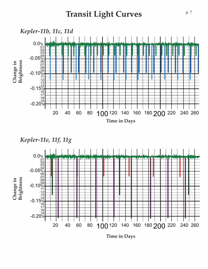
Kepler-11b, c, d

Transit Light CurvesC

hang

e in

Brig

htne

ss

Kepler-11e, 11f, 11g

Change in 

Brightness

0.0%

­0.05%

­0.10%

Time (in days)

4020 60 80 100120 140 200160 180 220 240 260

.01

.02

.03

.04

.06

.07

.08

.09

.11

.12

.13

.14

280

.14

.16

.17

.18

.19­0.20%

­0.15%

Kepler-11e, f, g

Time in Days

Kepler-11b, 11c, 11d

Cha

nge

inBr

ight

ness

Time in Days

Transit Tracks p. 8Change in 

Brightness

0.0%

­0.05%

­0.10%

Time (in days)

40

20

60

80100120140

200

160180

220

240260

.01

.02

.03

.04

.06

.07

.08

.09

.11

.12

.13

.14

280

.14

.16

.17

.18

.19

­0.20%

­0.15%

b

cd

e

g

f

Kepl

er-1

1b, c

, d, e

, f, g

Tim

e in

Day

s

Kep

ler-

11b,

11c

, 11d

, 11e

, 11f

, 11g

Change inBrightness

Transit Tracks p. 9

Planet Period Orbital DistanceName (Units ____________ Units ___________

Names:

Analyzing Light Curves

Orbital Distance (from Kepler’s 3rd Law graph)

Planet’s Size(planet radius using formula)

Brightness √Z Radius = 10 x √Z Drop of Z (%) (in Earth radii)

Planet

Questions: 1. Which planet(s) are similar in size to Earth?

2. Jupiter’s radius is about 11 times Earth’s radius. Which planets are similar in size to Jupiter?

3. Describe the relationship between the period of the planets and their orbital distances.

Transit Tracks: Student Worksheet © 2008 by the Regents of the University of California

Instructions: The “Transit Light Curves” are graphs of NASA’s Kepler Mission’s observations of stars. They show how the light level changes when a planet transits in front of a star. Study the light curves to find the period of the planet.The period is the time between transits and is year-length for a planet. Use “Kepler’s 3rd Law Graphs” to find the “Orbital Distance” of the planet from its parent star.

T h e “ P l a n e t ’ s S i z e ” i s f o u n d b y measuring the “Change in Brightness,” the small percentage drop in the light level as the planet transits. Calculate the planet’s radius using the formula in the table below.

Transit Tracks p. 10K

eple

r’s 3

rd L

aw G

raph

s

Kep

ler’s

3rd

Law

Gra

ph fo

r Per

iods

less

than

10

days

Kep

ler’s

3rd

Law

Gra

ph fo

r Per

iods

Les

s Th

an 1

00 D

ays

Kep

ler’s

3rd

Law

Gra

ph fo

r the

Inne

r Sol

ar S

yste

m

(per

iods

less

than

2 y

ears

)

Tran

sit T

rack

s: S

tude

nt W

orks

heet

©

200

8 by

the R

egen

ts of

the U

nive

rsity

of C

alifo

rnia

Transit Tracks p. 11

For stars the same size as the Sun, Kepler’s 3rd Law is simply:

R3 = T2 * or For the Sun, Ms = 1. For other stars, Ms is mass in rela-tionship to the Sun’s mass. The “Planet’s Size” is determined by measuring the “Change in Brightness,” the percentage drop in the light level as the planet transits. Calculate the planet’s radius using the formula in the table below.

Names:

CUBE ROOTSNumber Cube Root

0.0025 0.136

0.0050 0.171

0.0075 0.196

0.0010 0.100

0.0100 0.215

0.02 0.271

0.03 0.311

0.04 0.342

0.05 0.368

0.06 0.391

0.07 0.412

0.08 0.431

Number Cube Root Number Cube Root

0.09 0.448

0.1 0.464

0.12 0.493

0.14 0.519

0.16 0.543

0.18 0.565

0.2 0.585

0.22 0.604

0.24 0.621

0.26 0.638

0.28 0.654

0.3 0.669

0.32 0.684

0.34 0.698

0.36 0.711

0.38 0.724

0.4 0.737

0.5 0.794

0.6 0.843

0.7 0.888

0.8 0.928

1 1.000

Analyzing Light Curves: Calculated with Kepler’s 3rd Law

* Note: There is actually a constant K implied in this equation that sets the units straight: R3/T2 = K where K = 1 AU3/Year2

Planet’s Size(radius using formula)

Brightness √Z Radius = 10 x √Z Drop of Z (%) (in Earth radii)

Planet

Orbital Distancefrom Kepler’s 3rd Law

Questions: 1. Which planet(s) are similar in size to Earth?

2. Jupiter’s radius is about 11 times Earth’s radius. Which planets are similar in size to Jupiter?

3. Describe the relationship between the period of the planets and their orbital distances.

Transit Tracks: Student Worksheet © 2008 by the Regents of the University of California

Planet Period (T) T2 Ms R = √T2 Ms

Units: _______ Units: ________

3

For cube-root calculator instructions: http://kepler.nasa.gov/education/cuberoot/

Instructions: The “Transit Light Curves” are graphs of NASA’s Kepler Mission’s observations of stars. They show how the light level changes when a planet transits in front of a star. Study the light curves to find the period of the planet. The period is the time between transits and equals year-length for a planet (T). Like Johannes Kepler did, we express the planet’s distance (R) in Astronomical Units (AU). 1 AU is the average distance from the Earth to the Sun.

Transit Tracks p. 12

Plut

o

Nep

tune

Ura

nus

Satu

rn

Jupi

ter

Kep

ler’s

3rd

Law

for

Who

le S

olar

Sys

tem

: p

lane

ts, a

ster

oids

, dw

arf

plan

ets

(Lin

ear S

cale

s)

Transit Tracks p. 13

5040

3020

7060

105

43

28

76

10.

50.

60.

40.

30.

20.

1

1000 500

400

300

200

600

100 50 40 30 2060 10 5 4 3 26 1

0.5

0.4

0.3

0.2

0.6

0.1

0.050.07

0.06

Mer

cury

Venu

sEart

h

Mar

s

Ast

eroi

d Be

ltJupi

ter

Satu

rn

Ura

nusN

eptu

nePl

uto

Kep

lers

’s 3r

d La

w G

raph

of W

hole

Sol

ar S

yste

m w

ith L

ogar

ithm

ic S

cale

s

R =

Orb

ital R

adiu

s (A

U) [

Sem

i-maj

or a

xis]

T = Orbital Period (years)

100

Kep

ler’

s 3rd

Law

R3 =

T2

R, in

Yea

rs

T, in

Ast

rono

mic

al U

nits

, AU

Not

e: A

ll ob

ject

s -- p

lane

ts, m

oons

, ast

eroi

ds, c

omet

s, m

eteo

roid

s, dw

arf p

lane

ts --

all

obey

Kep

ler’s

3rd

Law

.

Transit Tracks p. 14Jeremiah Horrocks Makes First Observation of the Transit of Venus:

A transit of Venus across the Sun takes place when the planet Venus passes directly between the Sun and Earth, so that Venus blocks a small spot of the Sun’s disk. Since the Sun is over 100 times larger in diameter than Venus, the spot is very small indeed.

An Englishman, Jeremiah Horrocks, made the first European observation of a transit of Venus from his home in Much Hoole, England, in the winter of 1639. Horrocks had read about Johannes Kepler who predicted tran-sits in 1631 and 1761, and a near miss in 1639 when Venus would pass very close to the Sun, but not actually in front of it.

Horrocks made corrections to Kepler’s calculation for the orbit of Venus and predicted that 1639 would not be a near miss, but an actual transit. He was uncertain of the exact time, but calculated that the transit would begin about 3:00 pm. He focused the image of the Sun through a simple telescope onto a card, where the im-age could be safely observed. After watching for most of the day with clouds obscuring the Sun often, he was lucky to see the transit as clouds cleared at about 3:15 pm, just half an hour before sunset. The observations allowed him to make a well-informed estimate as to the size of Venus, but more importantly, using geometry, to calculate the distance between the Earth and the Sun which had not been known accurately at that time. He was the first of many people who used transit observations to try to determine the distance from the Sun to the Earth.

More About Jeremiah Horrocks and His Observations:Accounts of Horrocks’ (Horrox’s) observations were published in Latin, as was the common practice in the 17th century. “Venus in sole visa” was published many years after Horrocks’ death (at age 22) by Johannes Hevelius. An English translation of Horrocks’ notes on the transit are posted here: http://www.venus-transit.de/1639/horrox.htm

A short account of his short life, and his observations of the transit of Venus: http://www.transit-of-venus.org.uk/history.htm

Jeremiah Horrocks’ drawing of the transit of Venus, 1639.

Jeremiah Horrocks observing the transit of Venus, artist’s conception. (Public domain).

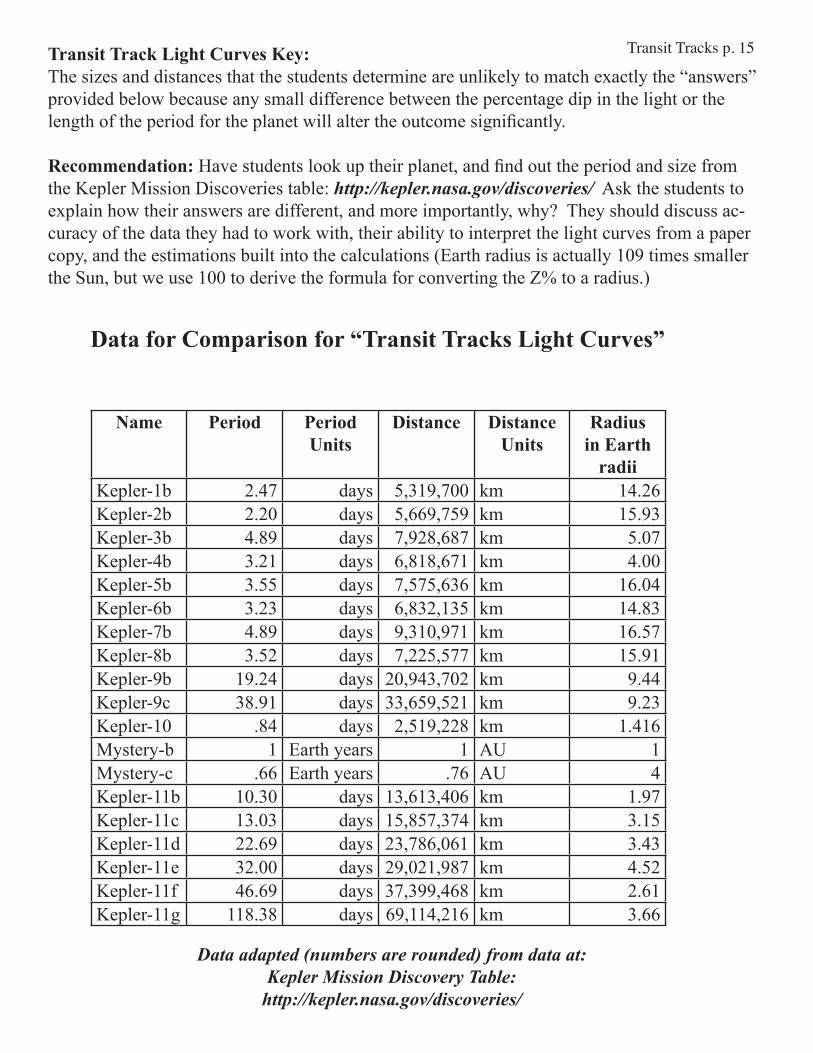
Transit Tracks p. 15Transit Track Light Curves Key:The sizes and distances that the students determine are unlikely to match exactly the “answers” provided below because any small difference between the percentage dip in the light or the length of the period for the planet will alter the outcome significantly.

Recommendation: Have students look up their planet, and find out the period and size from the Kepler Mission Discoveries table: http://kepler.nasa.gov/discoveries/ Ask the students to explain how their answers are different, and more importantly, why? They should discuss ac-curacy of the data they had to work with, their ability to interpret the light curves from a paper copy, and the estimations built into the calculations (Earth radius is actually 109 times smaller the Sun, but we use 100 to derive the formula for converting the Z% to a radius.)

Data for Comparison for “Transit Tracks Light Curves”

Name Period Period Units

Distance Distance Units

Radius in Earth

radiiKepler-1b 2.47 days 5,319,700 km 14.26Kepler-2b 2.20 days 5,669,759 km 15.93Kepler-3b 4.89 days 7,928,687 km 5.07Kepler-4b 3.21 days 6,818,671 km 4.00Kepler-5b 3.55 days 7,575,636 km 16.04Kepler-6b 3.23 days 6,832,135 km 14.83Kepler-7b 4.89 days 9,310,971 km 16.57Kepler-8b 3.52 days 7,225,577 km 15.91Kepler-9b 19.24 days 20,943,702 km 9.44Kepler-9c 38.91 days 33,659,521 km 9.23Kepler-10 .84 days 2,519,228 km 1.416Mystery-b 1 Earth years 1 AU 1Mystery-c .66 Earth years .76 AU 4Kepler-11b 10.30 days 13,613,406 km 1.97Kepler-11c 13.03 days 15,857,374 km 3.15Kepler-11d 22.69 days 23,786,061 km 3.43Kepler-11e 32.00 days 29,021,987 km 4.52Kepler-11f 46.69 days 37,399,468 km 2.61Kepler-11g 118.38 days 69,114,216 km 3.66

Data adapted (numbers are rounded) from data at: Kepler Mission Discovery Table:

http://kepler.nasa.gov/discoveries/