Investigation of voltage stability improvement inthe distribution network with large amount ofinduction motors using PSS/E: Loadinterruption and use of SVCs

Master of Science Thesis in the Master’s Degree Program, Electric Power Engineering

Sandra Milena Moreno CastilloJagger Hamulili Bwembelo

Department of Energy & EnvironmentDivision of Electric Power EngineeringChalmers University of TechnologyGothenburg, Sweden 2014

THESIS FOR MASTER OF SCIENCE

Investigation of voltage stability improvement inthe distribution network with large amount of in-duction motors using PSS/E: Load interruptionand use of SVCs

Sandra Milena Moreno Castillo

Jagger Hamulili Bwembelo

Department of Energy & EnvironmentDivision of Electric Power Engineering

Chalmers University of TechnologyGothenburg, Sweden 2014

Investigation of voltage stability improvement in the dis-tribution network with large amount of induction motorsusing PSS/E: Load interruption and use of SVCs

Sandra Milena Moreno Castillo

Jagger Hamulili Bwembelo

c©SANDRA MILENA MORENO CASTILLO, JAGGER HAMULILI BWEMBELO, 2014

Department of Energy & EnvironmentDivision of Electric Power EngineeringChalmers University of TechnologySE-412 96 Gothenburg, Sweden

Telephone:+46 (0)31-7721000Fax:+46 (0)31-7721633

Cover: Load interruption of 40% of non-motor loads together with load shedding of 60%of motor loads.Figure 5.17 (a).

Chalmers Bibliotek, ReproserviceGothenburg, Sweden 2014

Investigation of voltage stability improvement in the distributionnetwork with large amount of induction motors using PSS/E: Loadinterruption and use of SVCs

Sandra Milena Moreno CastilloJagger Hamulili Bwembelo

Department of Energy & Environment

Division of Electric Power Engineering

Chalmers University of Technology

Abstract

Voltage stability improvement methods following a disturbance and Fault Induced De-layed Voltage Recovery (FIDVR) event are studied with the aim of satisfying a voltagerecovery criterion and saving as much load as possible. These methods are temporaryload interruption and the use of Static Var Compensators (SVCs). The loads are tem-porarily tripped and then reconnected. The locations and sizes of SVCs are also deter-mined. The criterion to be met is the recovery of voltages at all buses in the network to0.9 pu within 1 s following a disturbance. Simulations are done on a typical distributionsystem with a large number of motor loads using Power System Simulator for Engineer-ing (PSS/E) software with the help of Python programming language for automationand control and the results are analyzed. The results show that load interruption aidsand significantly improves the voltage recovery following a disturbance in the network. Itis also observed from the results that the use of SVCs also enables the voltage to recoverfaster with the criterion for voltage recovery at all buses fulfilled. However, the bestresults are obtained when load interruption is combined with the use of SVCs. The twomethods complement each other. When the two methods are combined the amount ofload that has to be interrupted is less and the number of SVCs required is also reduced.This results in fewer loads being interrupted. Moreover, the investment cost on SVCs isalso reduced.

Index Terms: Voltage stability, Fault Induced Delayed Voltage Recovery (FIDVR),load interruption, Static Var Compensator (SVC).

i

ii

Acknowledgements

This report would not have been possible without the support of many people. Theauthors wish to express their gratitude to their supervisor, Dr.Tuan Le who was abun-dantly helpful and offered invaluable assistance, support and guidance. Special thanksto Prof. Thierry Van Cutsem from University of Liege for his support and provision ofnetwork data. Thanks to Pavan Balram for his help and support during the process ofthis thesis.

Jagger would like to thank his wife Phyllis, his son Joseph and his daughter Lois fortheir support, encouragement, patience and prayers during the period that he was awayundertaking the Master’s Degree program. They have been a source of inspiration. Hewould also like to thank Chalmers and the Chalmers Foundation for awarding him theAvancez scholarship as well as his employers, ZESCO Limited, for granting him studyleave which has enabled him to pursue the Master’s Degree program.

Esta tesis se la quiero dedicar especialmente a la memoria de mi amado padre AdanMoreno Salamanca, que aunque no este conmigo fisicamente, se que el siempre estuvoorgulloso de mı y siempre quiso que esta maestrıa se hiciera realidad. Gracias Papito teamare por siempre. Deseo expresar infinitas gracias a mi familia por su apoyo incondi-cional y ayuda durante estos anos de estudios. Muchas gracias a mı amado Eduardopor su amor y comprension ya que sin el esta maestrıa no hubiera sido posible. Milinfinitas gracias Mamita Sofıa, tu me has ensenado a luchar y perseverar por las cosasimportantes de la vida, sin ti y mi papa yo no serıa la persona que soy hoy, los amo y mesiento afortunada de la familia que construyeron para mı, mis hermanos y mi Eduardo.Muchas gracias a mis queridos hermanos German y Edgar por su acompanamiento eincondicional amor, a mi abuelita Tulia que la quiero mucho y a la familia Castillo enespecial a mis tıos Carlos, Idelfonso y Edilma a Sandra, Diego, Isabela, Marıa Helenapor su amor y acompanamiento.

Muchas gracias a la familia Moreno, gracias primos, tıos, amigos por su apoyo y amor encada una de los recibimientos y despedidas en Colombia; esos buenos momentos hicierondurante este tiempo, la vida mas facil lejos de mi tierra. Mi querida tıa Rosa gracias por

iii

ser tan tierna y linda conmigo de igual manera a mis tıas Marıa y Brıgida.

Finalmente y no memos importante quisiera gradecer a mi amigo del alma John CarlosMolina por su amistad incondicional y acompanamiento, senora Lucila y Cecilia Azagracias por el apoyo durante este tiempo.

Sandra Milena Moreno Castillo

Jagger Hamulili Bwembelo

Gothenburg, Sweden, 2014

iv

v

Contents

Abstract v

Acknowledgements v

Contents v

List of symbols, abbreviations and acronyms viii

1 Introduction 11.1 Project Background . . . . . . . . . . . . . . . . . . . . . . . . . . . . . . 11.2 Project Objective/Aim . . . . . . . . . . . . . . . . . . . . . . . . . . . . . 21.3 Tasks . . . . . . . . . . . . . . . . . . . . . . . . . . . . . . . . . . . . . . 21.4 Scope . . . . . . . . . . . . . . . . . . . . . . . . . . . . . . . . . . . . . . 31.5 Organization of the thesis . . . . . . . . . . . . . . . . . . . . . . . . . . . 3

2 Literature Review 62.1 Voltage stability . . . . . . . . . . . . . . . . . . . . . . . . . . . . . . . . 62.2 Measures for improving Voltage Stability . . . . . . . . . . . . . . . . . . . 92.3 Undervoltage Load Shedding Using Distributed Controllers . . . . . . . . 132.4 Load shedding and Tap Changer Blocking with information from genera-

tor Over Excitation Limiters (OELS) . . . . . . . . . . . . . . . . . . . . . 142.5 Load shedding based on predictive control . . . . . . . . . . . . . . . . . . 142.6 Load shedding using induction motor kinetic energy . . . . . . . . . . . . 152.7 A combination of load shedding and the use of SVCs . . . . . . . . . . . . 152.8 Event based load shedding . . . . . . . . . . . . . . . . . . . . . . . . . . . 152.9 Static Var Compensator (SVCs) . . . . . . . . . . . . . . . . . . . . . . . 16

3 Induction Motor Model 203.1 Induction motor . . . . . . . . . . . . . . . . . . . . . . . . . . . . . . . . 203.2 Simulation process of an induction motor as a bus load in PSS/E . . . . . 213.3 Equivalent circuit . . . . . . . . . . . . . . . . . . . . . . . . . . . . . . . . 21

vi

3.4 Induction motor models . . . . . . . . . . . . . . . . . . . . . . . . . . . . 223.5 Induction Motor Load Model CIM5BL . . . . . . . . . . . . . . . . . . . . 233.6 IMD application tool . . . . . . . . . . . . . . . . . . . . . . . . . . . . . . 243.7 Motor type 1 . . . . . . . . . . . . . . . . . . . . . . . . . . . . . . . . . . 253.8 The integration time step ∆t . . . . . . . . . . . . . . . . . . . . . . . . . 25

4 Load flow and dynamic simulation using PSS/E 264.1 Directories and Files Overview . . . . . . . . . . . . . . . . . . . . . . . . 274.2 Steady-state load flow . . . . . . . . . . . . . . . . . . . . . . . . . . . . . 284.3 Dynamic simulation connection of the induction machines (IMD) . . . . . 294.4 Python programming language . . . . . . . . . . . . . . . . . . . . . . . . 32

5 Improvement of voltage stability by temporary load interruption 345.1 Simulations without load interruption . . . . . . . . . . . . . . . . . . . . 365.2 Non-motor load shedding . . . . . . . . . . . . . . . . . . . . . . . . . . . 375.3 Load shedding of various percentages of non-motor and motor loads. . . . 40

5.3.1 10% load shedding of motors . . . . . . . . . . . . . . . . . . . . . 415.3.2 20% load shedding of motors . . . . . . . . . . . . . . . . . . . . . 435.3.3 40% load shedding of motors . . . . . . . . . . . . . . . . . . . . . 445.3.4 80% load shedding of motors . . . . . . . . . . . . . . . . . . . . . 45

5.4 Load interruption of 40%, 60% and 80% of non-motor loads . . . . . . . . 455.5 Load interruption of 40%, 60% and 80% of non-motor loads together with

load shedding of 60% of motor loads. . . . . . . . . . . . . . . . . . . . . . 49

6 Improvement of voltage stability by using SVCs 516.1 Simulation results . . . . . . . . . . . . . . . . . . . . . . . . . . . . . . . 56

6.1.1 SVC placed at Node 11C . . . . . . . . . . . . . . . . . . . . . . . 566.1.2 SVC connected to Node 11B and 11C . . . . . . . . . . . . . . . . 606.1.3 SVC connected to Node N11AC5 . . . . . . . . . . . . . . . . . . . 626.1.4 SVCs connected to Node 13C, 13B, 11C, 11B, 10C, 10B, 8C, 8B,

7C, 7B, 5C and 5B . . . . . . . . . . . . . . . . . . . . . . . . . . . 656.1.5 SVC placed at Node N11A . . . . . . . . . . . . . . . . . . . . . . 676.1.6 SVCs placed at Node 11A and 13A . . . . . . . . . . . . . . . . . . 696.1.7 SVCs placed at Node 4A, 11A and 13A . . . . . . . . . . . . . . . 716.1.8 SVCs placed at Node 4A, 5A, 11A and 13A . . . . . . . . . . . . . 73

7 Improvement of voltage stability by combining load interruption withusing SVCs 767.1 Simulations Results . . . . . . . . . . . . . . . . . . . . . . . . . . . . . . . 76

8 Improvement of voltage stability by load shedding using the PSS/EUndervoltage Load Shedding Model Relay 808.1 Simulation results . . . . . . . . . . . . . . . . . . . . . . . . . . . . . . . 80

vii

9 Conclusions and Future Work 849.1 Conclusions . . . . . . . . . . . . . . . . . . . . . . . . . . . . . . . . . . . 849.2 Future Work . . . . . . . . . . . . . . . . . . . . . . . . . . . . . . . . . . 85

References 90

A Distribution Network 91

B Python Scripts 92

viii

List of symbols, abbreviationsand acronyms

BUS NAME : Name of the bus to which element is connected.MVA : Mega-Volt-Ampere.SBASE : System MVA base.ID : Element identifier.ZONE : Zone to which the element is assigned.AREA : Area to which the element is assigned.OWNER : Owner to which the element is assigned.∆t: Integration time step.

EXCITER

TE : Time constant, in seconds (s).EMIN : Minimum field voltage, in pu [1].EMAX : Maximum field voltage, in pu.K : The gain.

DOUBLE-CAGE INDUCTION MOTORS

MBASE : Machine base power.RA: Armature resistance, in pu on motor base.XA: Armature leakage inductance, in pu on motor base.XM : Magnetizing inductance, in pu on motor base.R1: Resistance of first rotor winding, in pu on motor base.X1: Reactance of the first rotor winding, in pu on motor base.R2: Resistance of second rotor winding, in pu on motor base.X2: Reactance of the second rotor winding, in pu on motor base.

ix

H : Inertia constant, pu motor base.Tnom: Load torque at 1 pu speed.D : Load damping factor.

ACRONYMS

FIDVR: Fault Induced Delayed Voltage Recovery.SVC : Static Var Compensator .PSS/E: Power System Simulator For Engineering.UVLS: Under Voltage Load Shedding.FACTS: Flexible AC Transmission Systems.STATCOM: Static Synchronous Compensator.SVG: Static VAR GeneratorSIPS: System Integrity Protection Scheme.SPS: Special Protection System (also referred to as System Protection Scheme)OEL: Over Excitation Limiter.LTC: Load tap changer.SPS: Special Protection System.VSA: Voltage security assessment.AVR: Automatic Voltage Regulators.PSS: Power System Stabilizer.EHV: Extra High Voltage.GENCO: Generating Company.TSO: Transmission System Operator.MEL: Most Effective Load.

x

1Introduction

1.1 Project Background

Nowadays, power systems are operated closer to their stability limits due toderegulation and challenges in constructing new transmission lines and powerstations [2]. At the same time, there has been an increase in the usage ofmotors in air conditioners, refrigerators and heat pumps as well as voltage-

insensitive loads that have electronic supplies. This makes power systems to be proneto voltage instability problems [3].

Fault-induced delayed voltage recovery (FIDVR) is a trend that has been observed inpower systems with a high penetration of induction motor loads following a fault. FIDVRis defined as “the phenomenon whereby system voltage remains at significantly reducedlevels for several seconds after a fault in transmission, sub-transmission, or distributionsystem has been cleared” [4]. This problem is mainly caused by motor load re-accelerationafter a fault in the nearby transmission system which causes a severe voltage drop. Thisleads to motor loads drawing high current from the grid which causes even more voltagedrop. In the worst case, motors may stall which results in the voltage instability problem[5]. Generators and Load Tap Changers (LTCs) on transformers can sometimes reachtheir limits of allowed control range following a severe voltage drop. LTC movement canalso be too slow[6].

Some of the notable early FIDVR events in North America are the Tennessee ValleyAuthority (TVA) Service Area cascading voltage collapse in August 1987, Florida Powerand Light Company (FPL)’s Miami area in August 1988 and Southern California Edi-son’s (SCE) network (in 1988 and in SCE’s desert regions in June 1990). During theseevents motors (pumps and /or air conditioners) either tripped on thermal and overloadprotection or stalled drawing a lot of current[4]. Some major incidents related to voltageinstability are the French system disturbance (December 19, 1978 and January 12, 1987),

1

Northern Belgium system disturbance (on August 4, 1982), Florida system disturbance(December 28, 1982) and WSCC USA (July 2, 1996) [7]. Other major incidences are NEof USA/Canada blackout (August 14, 2003), blackout in southern Sweden and EasternDenmark (September 23, 2003) and the Polish system disturbance (June 26, 2006) [3].

Temporary load interruption with load shedding as backup has been proposed in [5] foraverting FIDVR or voltage instability. It can aid the recovery of the voltage after a dis-turbance which helps the motors to re-accelerate and the stalling of some of the motorscan also be avoided. The load is switched off and then reconnected after a short timeinterval or if the voltage recovers above the value that has been set [5]. Load shedding isthe last resort to prevent voltage instability when all else fails [7, 8]. It is a cost effectiveway to mitigate voltage instability[9]. However, the load is not reconnected after beingshed therefore it is not saved as is the case with load interruption. Thus, other means ofaiding the voltage recovery can also be combined with load interruption so that as muchload as possible is saved and load shedding is minimized. One of the methods that can beinvestigated is the combination of load interruption and the use of FACTS devices suchas Static Var Compensators (SVC). SVCs have also been used to aid voltage recoveryfollowing disturbances to prevent voltage instability such as in [10].

1.2 Project Objective/Aim

The aim of this thesis is to study voltage stability improvement in a distribution networkwith a large amount of induction motors by a combination of temporary load interrup-tion and using SVCs so as to counteract the problem of FIDVR and save as much loadas possible. During this thesis a generic algorithm/approach will be developed in orderto determine the amount of load to be interrupted and the time-interval to mitigate thevoltage instability problem. In order to establish these, the time-dependent relationshipbetween voltage and power interruption (both active and reactive power) will be derivedand utilized in the algorithm. The use of SVCs to aid the voltage recovery and reduce theamount of interrupted load will also be investigated. The size and locations of the SVCswill also be determined. A case study will be done on a test network. Dynamic simu-lations of the system will be performed in the Power System Simulator for Engineering(PSS/E) software and the performance of the methods/approach will be tested.

1.3 Tasks

The main tasks during this thesis revolve around the development of a generic algo-rithm/approach in order to determine the minimum amount of load to be interruptedand the interruption time as well as investigating the use of SVCs in order to preventthe voltage instability problem. The two methods of preventing voltage instability willthen be combined and the results analyzed.

The following are the activities that have been carried out during the period of the thesis,

2

1. Literature review on voltage stability

2. Literature review on existing system protection schemes for the improvement ofvoltage stability.

3. Survey of existing algorithms for protection against voltage instability such asunder-voltage load shedding, etc.

4. Literature review on SVCs

5. Learning to use PSS/E simulation tool for dynamic simulation.

6. Performing load flow and dynamic simulations of a test-model of a distributionsystem with a high share of motor loads in PSS/E.

7. Development of an analytical formula or approach for temporally load interruptionto determine the minimum amount of load to be interrupted and the interruptiontime.

8. Implementation of the test-model network and the approach/method developedin Task-7 in PSS/E. Carrying out simulation runs for various scenarios of loadinterruption.

9. Implementation of the test-model network with SVCs in PSS/E. Determination ofsizes and location of SVCs.

10. Implementation of the test-model network with SVCs and the approach/methoddeveloped in Task-7 for temporally load interruption for the mitigation of thevoltage instability problem.

11. Final thesis report and presentation at Chalmers.

1.4 Scope

The thesis covers the development of an analytical formula or approach to determinethe minimum amount of load to be interrupted and the interruption time as well as itsimplementation in PSS/E for the prevention of voltage instability. It also covers the useof SVCs to counteract the voltage instability problem. The location and sizes of theSVCs are also determined. The two methods are combined and studied. Load flow anddynamic simulations of the system are done during this work.

1.5 Organization of the thesis

In this thesis different methods of improving voltage stability will be used in order toachieve a fast voltage recovery after a disturbance is introduced in the test network.The criteria used in this thesis is that voltage should recover to 0.9 pu within 1 s. In

3

order to achieve this target different methods and scenarios will be simulated such asload shedding, load interruption, SVCs and different combinations of these methodswill be considered. The organization of the thesis has been made in such a way that thereader finds an introduction, literature review of different methods for improving voltagestability, results of the simulations of different methods and scenarios, conclusion andfuture work. The layout of the thesis is as follows:

1. Chapter 1: Gives an introduction of the project background.

2. Chapter 2: Provides literature review on voltage stability and different methodsthat are used to improve voltage stability.

3. Chapter 3: In this chapter it is well explained how the induction machines havebeen simulated in PSS/E.

4. Chapter 4: Gives an overview on the simulation setup and implementation inPSS/E. A brief description of how to perform load flow and dynamic simulationsin PSS/E is also given.

5. Chapter 5: In this chapter the results for improving voltage stability by loadinterruption are presented.

6. Chapter 6: In this chapter the results for improving voltage stability by using SVCsare presented.

7. Chapter 7: In this chapter the results for improving voltage stability by a combi-nation of load interruption and the use of SVCs are presented

8. Chapter 8: In this chapter the results for improving voltage stability by using anunder-voltage relay are presented.

9. Chapter 9: The conclusions of the work are stated as well as the future work.

The methodology of how the voltage stability improvement investigations were carriedout is illustrated in Fig. 1.1

4

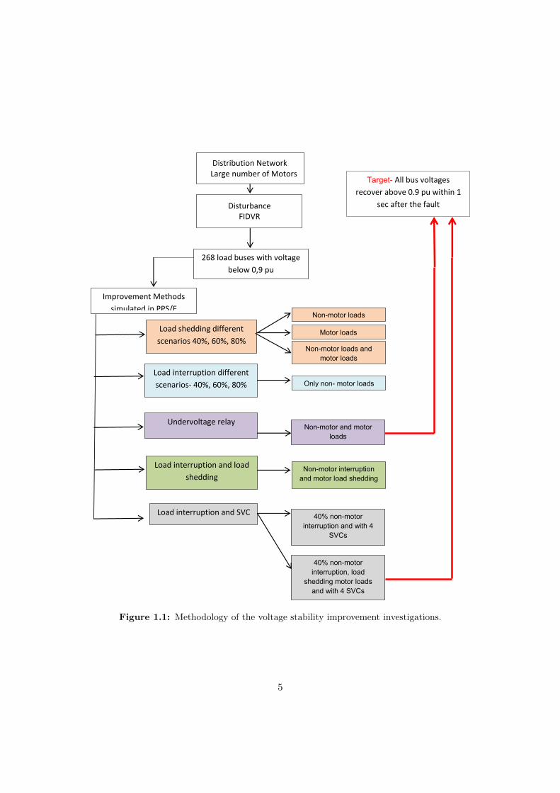
268 load buses with voltage below 0,9 pu

Distribution Network Large number of Motors

Load shedding different scenarios 40%, 60%, 80%

Load interruption and load shedding

Disturbance FIDVR

Improvement Methods simulated in PPS/E

Load interruption different scenarios- 40%, 60%, 80%

Undervoltage relay

Non-motor loads

Only non- motor loads

Non-motor and motor loads

Non-motor interruption and motor load shedding

Motor loads

Non-motor loads and motor loads

Load interruption and SVC 40% non-motor interruption and with 4

SVCs

40% non-motor interruption, load

shedding motor loads and with 4 SVCs

Target- All bus voltages recover above 0.9 pu within 1

sec after the fault

o.9

Figure 1.1: Methodology of the voltage stability improvement investigations.

5

2Literature Review

This chapter gives an overview from the literature of voltage stability, the mainfactors that lead to voltage instability and the measures to improve voltagestability. Literature review on the FIDVR phenomenon is also presented inthis chapter. A number of technical papers have been written with various

proposals on how to mitigate the FIDVR phenomenon. Research in this field is ongoing.Some of the proposals and schemes currently in use are categorized and highlightedbelow. The theory behind Static Var Compensators (SVCs) is also presented in thischapter since simulations have been done to study their effect in aiding the voltagerecovery following a disturbance.

2.1 Voltage stability

Voltage stability is whereby the system is capable of sustaining stable voltages at allbuses in a network following a disturbance [11]. Voltage instability is when voltages in anetwork considerably drop continuously to the point where the system becomes unstableand supply of power to the load is disturbed. This may lead to voltage collapse. Thetendency of load dynamics to reinstate the amount of power consumed post-disturbanceto a level that cannot be supplied by the generators and transmission system is whatbrings about the instability. Voltage stability has received a lot of attention in recentyears because events such as blackouts attributed to voltage instability have happenedaround the world and more are likely to occur. Power systems are operating closer totheir limits which make them more predisposed to voltage instability [12]. A significantpart of this section comes from [12] where voltage instability has been extensively dis-cussed with references from various sources.

A number of issues have led to power systems being more prone to voltage instabil-ity. One of the reasons is that it is getting harder to get permission to construct new

6

power stations and transmission lines. The result is that power stations are being builtfurther away from the load in remote areas thereby increasing the electrical distance.Shunt compensation can increase the amount of power that is transmitted. However,this comes at the expense of bringing the normal operating point nearer to the stabilitylimit. Unplanned outages of generators and transmission lines can also lead to volt-age instability. Another contributing issue is that there is economic impetus to operatepower systems near their limits due to deregulation of power markets. Establishing thevoltage stability limits of a system also becomes necessary as a result of this need [12].

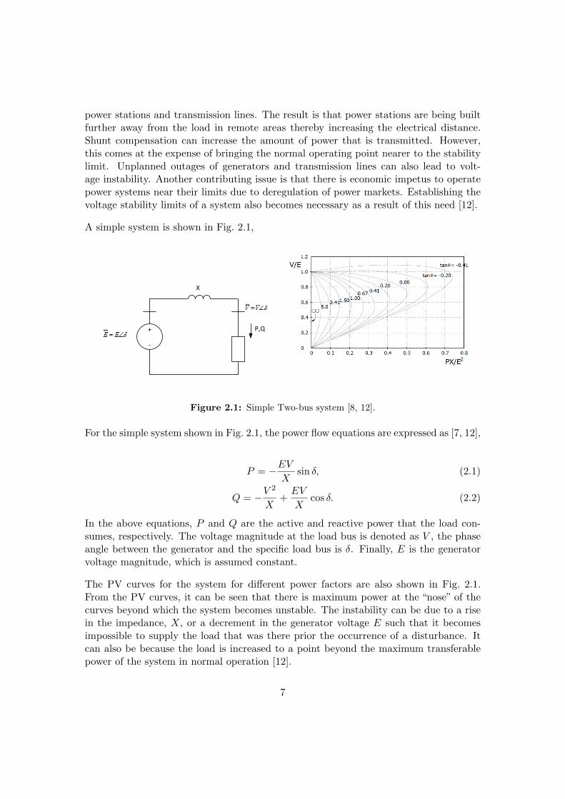
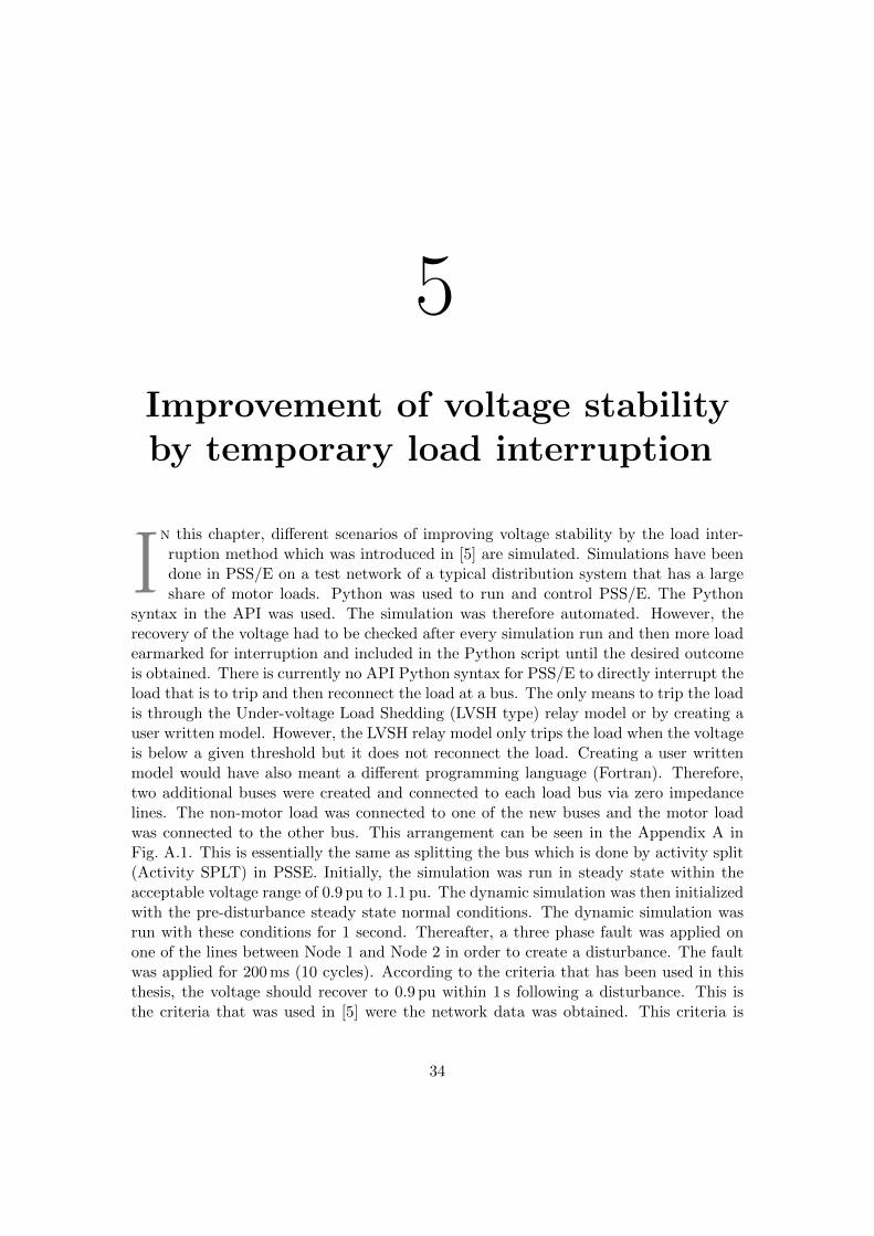
A simple system is shown in Fig. 2.1,

X

P,Q+

-

Figure 2.1: Simple Two-bus system [8, 12].

For the simple system shown in Fig. 2.1, the power flow equations are expressed as [7, 12],

P = −EVX

sin δ, (2.1)

Q = −V2

X+EV

Xcos δ. (2.2)

In the above equations, P and Q are the active and reactive power that the load con-sumes, respectively. The voltage magnitude at the load bus is denoted as V , the phaseangle between the generator and the specific load bus is δ. Finally, E is the generatorvoltage magnitude, which is assumed constant.

The PV curves for the system for different power factors are also shown in Fig. 2.1.From the PV curves, it can be seen that there is maximum power at the “nose” of thecurves beyond which the system becomes unstable. The instability can be due to a risein the impedance, X, or a decrement in the generator voltage E such that it becomesimpossible to supply the load that was there prior the occurrence of a disturbance. Itcan also be because the load is increased to a point beyond the maximum transferablepower of the system in normal operation [12].

7

Long-term voltage stability comprises of the dynamics of equipment which take long toact such as tap-changing transformers, loads controlled by thermostats and generatorcurrent limiters [3]. Some of the causes of long-term voltage instability are the operationof Load Tap Changers (LTCs) of transformers and the action of over-excitation Limiters(OELs) of generators. Long-term voltage instability happens over some minutes [12]usually up to 10 minutes [3]. After a severe disturbance there could be a dramatic dropof voltages at load buses. The LTCs for the transformers supplying these loads wouldthen try to increase the voltages at these buses to be within the dead-band that hasbeen set. This results in the restoration of the load power. LTCs therefore eventuallymake the load to act like constant power load in the long run. However, this in turndepresses the voltages upstream in the transmission network. The voltages on the lowvoltage side of the transformers in the distribution network would initially increase buteventually the effect of the LTCs would be minimal or even opposite in that the voltagewould actually start to reduce with each LTC operation. This can happen if some of thegenerators in the area reach the limit of their field current with the result that OELsare activated. The generators whose OELs are activated are not able to provide furtherreactive power support and so the voltages at their buses drop and the maximum loadpower also reduces. The system after the disturbance might not be able to satisfy thisload restored by the LTCs due to a reduction in the maximum power which could leadto instability [12].

Thermostatically controlled loads can also lead to long-term voltage instability. Thesetypes of loads are self-restoring. In this type of electrical heating, the power reduces asthe square of the voltage if there is a reduction in voltage. The temperature is regulatedby the thermostat which turns the heating resistor on and off to maintain it. However,if there is a significant voltage drop in the network after an event such as a disturbancethen the heating resistor is kept on for a longer time to provide the same amount ofenergy or it is not turned off. If the number of heaters in the network is large then thisaction becomes similar to self-restoring loads though it can be like impedance load if thedrop in voltage is significant. Thermostatically controlled loads can have a considerableeffect on a network especially in winter if they constitute a substantial share of the load.The effect can also be pronounced if LTCs do not manage to raise the voltage closer tothe dead-band [12].

Short-term voltage stability comprises of the dynamics of elements of the load which actquickly such as induction motors, electronically controlled loads and HVDC converters[3, 13], . Short term instability occurs over some seconds [12] usually up to 10 s [3]. Thepresence of induction motors can lead to short-term instability. Induction motors areself-restoring loads. The active power of induction motors reduces as the square of thevoltage in a similar manner as constant impedance load. This can happen following adisturbance. The load can then return to almost the same level as it was before within1 s. It can even return to constant power in some cases. The reactive power reducessort of quadratically to a low point then recovers until motors stall because of depressedvoltage. This may happen at a voltage of 0.7 pu for large motors and a higher voltage

8

for small motors. The effect of induction motors restoring load can be high in summerat peak load in networks with a high penetration of air conditioners [12].

Long-term voltage stability is therefore characterized by the action of LTCs, OELs,switched shunt compensation and the restoration of the composite load as well as sec-ondary control of voltage and frequency [12]. On the other hand, the aspects of short-term voltage stability are generators, SVCs, Automatic Voltage Regulators (AVRs),Power System Stabilizers (PSSs), turbines and governors, induction motors, HVDC linksand FACTS devices such as SVCs [12] and STATCOM [14].

2.2 Measures for improving Voltage Stability

Certain measures can be undertaken to improve voltage stability. One of the measuresis system reinforcement. This can be done in a number of ways. New transmission linescan be built from the power stations to the load centers. New power stations can alsobe built closer to the load. However, owing to the difficulty of building new lines andpower stations close to populous areas where the load is concentrated due to issues to dowith protecting the environment as well as political reasons other measures to reinforcethe system can also be implemented. Series compensation enables the reduction of theimpedance of transmission lines thereby restraining the voltage drop for lengthy lines.In spite of these gains, factors such as cost and increase in complexity of protection haveto be checked and taken into account. Shunt compensation is a long-established meansof preserving the voltage profile within an acceptable range by the provision of reactivepower support [12].

It is well known that reactive shunt compensation enables a larger amount of powerto be transmitted in steady-state and the regulation of the voltage profile over a lineto a desired level. It is also used to improve the transient stability of a network byincreasing the transmittable power of the post-fault system as well as power oscillationdamping. The loading of the network on a typical day varies so the objective is to adjustthe characteristics of the line to meet the load at a given point of time. The type ofcompensation used depends on the current status of the system in terms of loading.Fixed or mechanically switched shunt reactors are used to reduce over-voltages that mayoccur when the system is lightly loaded. Shunt capacitors are used to raise the voltage toa predetermined level when the system is heavily loaded thereby preventing low voltagesin the system [15].

Shunt var compensation is used in the middle of a transmission line connecting two ACsystems that has more than one source of supply for line segmentation. This concept isillustrated in a two-machine transmission model. The voltage profile along the line is notuniform and the lowest voltage is at the middle point of the line. Therefore, connectionof shunt var compensator at this point gives the best result because the line is dividedinto two equal parts with the same amount of power transfer capability. The longerportion of the line determines the maximum transmittable power if the compensator is

9

not connected in the middle [15]. Transmittable active power is given by [15],

P =2V 2

Xsin(δ/2). (2.3)

Likewise, the reactive power is

Q =4V 2

X(1− cos(δ/2)) (2.4)

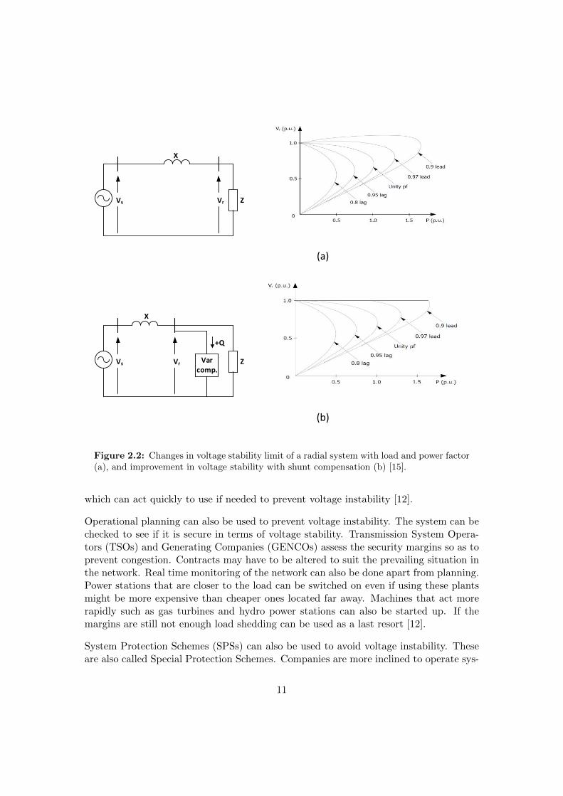
Transmittable power is increased twofold with mid-point shunt compensation. The volt-age profile also improves and becomes more uniform along the line. However, this entailsthe injection of more reactive power, which can increase up to fourfold, by the var com-pensator and the generators at the ends of the line. Line segmentation for voltagesupport using SVCs has been used in practice [15].

Shunt var compensation is also used at the end of a radial system. The terminal volt-age at the end of the line varies with the load and load power factor as illustrated inFig. 2.2(a) for the graph of normalized receiving voltage Vr versus normalized load powerP . This is the case without shunt compensation. The system is also shown in the figurewith line reactance X and load impedance Z. The nose-point of the plot for each of thecurves for the various power factors is the load at which voltage instability commences.As can be seen in the figure, the voltage drop is higher as the load increases. Further-more, the nose-point increases with capacitive loads and reduces with inductive loads[15].Fig. 2.2(b) shows the radial system with shunt var compensation at the receiving end ofthe line where the load is connected. The voltage is maintained at 1 p.u as can be seen inthe figure. The curves also show that shunt compensation can improve voltage stabilityby providing reactive power support. The voltage deviation is highest at the end of theline in a radial system. This is therefore the ideal place to connect the compensator [15].

Shunt compensation at the receiving end of a radial line is used for voltage support incase of the loss of a generator or one of the circuits supplying the load. This can alsohappen if, for instance, two lines from two different power stations are supplying an areaload and one of the lines trips. There would be a deficit of power if the system wasstretched prior to the disturbance. This could lead to voltage collapse [15].

Some devices and controllers are also used to improve voltage stability. SVCs can beused to prevent short-term voltage instability because they provide rapid reactive powersupport. Mechanically switched shunt compensation can be used to prevent long-termvoltage instability. The reactors that are used to lower the voltage for long unloadedExtra High Voltage (EHV) transmission lines can also be switched off so as to raise thevoltage. AVR set points for generators can be raised as well as using LTCs for generatorstep-up transformers to raise the voltage. The dynamic reactive power reserve of gen-erators, synchronous condensers and SVCs in a network can be increased by turning onshunt compensation. This leaves enough reactive power reserve available by equipment

10

Vs Vr

X

Z

(a)

Vs Vr

X

ZVarcomp.

+Q

(b)

Figure 2.2: Changes in voltage stability limit of a radial system with load and power factor(a), and improvement in voltage stability with shunt compensation (b) [15].

which can act quickly to use if needed to prevent voltage instability [12].

Operational planning can also be used to prevent voltage instability. The system can bechecked to see if it is secure in terms of voltage stability. Transmission System Opera-tors (TSOs) and Generating Companies (GENCOs) assess the security margins so as toprevent congestion. Contracts may have to be altered to suit the prevailing situation inthe network. Real time monitoring of the network can also be done apart from planning.Power stations that are closer to the load can be switched on even if using these plantsmight be more expensive than cheaper ones located far away. Machines that act morerapidly such as gas turbines and hydro power stations can also be started up. If themargins are still not enough load shedding can be used as a last resort [12].

System Protection Schemes (SPSs) can also be used to avoid voltage instability. Theseare also called Special Protection Schemes. Companies are more inclined to operate sys-

11

tems closer to their limits with the aim of maximizing profits because of deregulation.With this status quo the most likely scenario is to use security margins to take care ofcontingencies while SPSs can be used for more serious disturbances which do not oftenhappen. SPSs operate automatically to avert instability. SPSs can combine a numberof measures such LTC blocking, decrease of LTC set points to decrease the voltage,returning the tap positions of transformers to prearranged points or load shedding. Dis-tribution voltages can be lowered so as to reduce the load but sub-transmission voltagescan be raised so as to lower the losses and also take advantage of shunt compensation.Load shedding of small induction motors to improve short-term voltage stability is sup-posed to be rapid. Large motors have under-voltage protection so they trip relativelyfaster than smaller motors such as those found in air conditioners which use thermalprotection [12].

Power blackouts due to, for example, faults at power stations, damage to transmissionlines, short circuits and overloading in the generation or transmission systems (to namebut a few situations), can lead to the shedding of loads in selected parts of the electricnetwork in order to provide power flow at critical feeders such as hospitals, mines, treat-ment plants, etc. Different load shedding schemes are in use and proposed and some ofthem are mentioned hereafter.

When it comes to load shedding schemes, the system operator usually makes decisionsbased on concerns about the security of the system. Such concerns include voltage[16, 17], current, power, frequency limitations [18], and customer interruption costs [19].Taking into account the above mentioned factors, several articles addressed their re-search in developing an efficient method to minimize the load curtailment. To achievethat, in [20], the authors proposed a scheme based on static optimization (Kuhn-Tuckertheorem) for a 26-node example problem. Similarly, based on optimization, but usinginstead a Newton based dynamic algorithm, [21] presents a reformulated optimal loadshedding. Furthermore, linear and quadratic programming models have also been usedin [22, 23], as well as strategies based on genetic algorithms [24].

One article that studies dynamic load shedding including the load characteristics in ahighly interconnected and loaded electrical power system is [25]. This paper introducesa load shedding policy for generation load imbalances and formulates the problem interms of nonlinear programming problem. A recent proposal based on time optimal loadshedding is discussed in [21]. Concerning load shedding on a specific feeder, [26] analysesthe application of the Everett optimization scheme for value-based load shedding in anaval-ship power system. Adaptive load shedding to regulate unacceptable frequencydeviation is described in [27]. In this case, an islanded area consisting of one lumpedgenerator and turbine model is used. In case of load shedding for power systems withmultiple distributed generation, paper [28] tackles this problem. Based on the role ofdistributed generation in emergency state, the authors identified three scenarios in orderto study static and dynamic models. A combination of adaptive and intelligent shed-ding techniques for load shedding is the main topic of [29]. In this paper, the authors

12

described a new under-frequency load shedding method for an islanded distribution net-work. For a review about the main problems of load shedding concerning the integrationof wind turbines into power systems, the reader is referred to [30] and references thereinfor more details. Optimal load shedding in smart electric power grids is studied in Ref.[31]. Finally, concerning the economic aspects of load shedding, different articles can befound in the scientific literature among them we refer to [32]. As mentioned before thisreview is not complete or exhaustive.

To maintain power system security, it is advantageous to use and develop measures toimprove voltage stability. Indeed, during this thesis load interruption, load shedding,under-voltage relays, SVCs and a combination of load interruption and using SVCs willbe implemented in order to investigate the improvement in voltage stability. These mea-sures will be done in order to facilitate the machines that are still connected to thenetwork to re-accelerate after fault clearing.

2.3 Undervoltage Load Shedding Using Distributed Con-trollers

Load shedding schemes using distributed controllers have been proposed in [6]. Theextent and rate at which the voltage drops determines the amount of load to interrupt.No communication is required between controllers since they are distributed and operatebased on the status and progression of voltage drop in their zone. The amount ofload that is shed is proportional to the rate of voltage drop [6]. This load sheddingscheme falls under the classification of SPSs against long term voltage instability [33].The voltages at some transmission buses are monitored by individual controllers whichact on the respective load in the distribution network. The notable features of theproposed protection scheme are that it is response-based, rule-based, works on closed-loop operation and uses a distributed scheme. The characteristics of these features are[6]:

• Response-based: activation of load shedding is based on measurement of voltage.The source of the disturbance is not identified. The operation of other controllersis also taken into consideration.

• Rule-based: Load shedding is initiated if voltage drops below a threshold value fora certain period of time. The rate of voltage drop determines the amount of loadto shed.

• Closed-loop operation: The controllers check the voltage in their zone after theirinitial activation and determine whether to shed more load or not until the voltagegoes back to normal (above the threshold value). This enables them to adjust tothe significance of the disturbance.

• Distributed: The controllers are distributed so that those closest to the disturbanceare activated first because that’s where the voltage drop is more significant.

13

Another approach that is proposed in Ref.[34] is the combination of load interruptionand shedding using a System Integrity Protection Scheme (SIPS). The local controllersact on a distribution bus by first temporarily interrupting load (mainly non motor)connected to the same bus. Load shedding (of mainly motor load) is then initiated ifthe voltage does not recover above a time-varying threshold voltage or the limit of loadavailable for interruption is reached. The load is just disconnected and not reconnectedback in the second case (for motor load). The time-varying threshold voltage for loadinterruption is different from the one for load shedding and there is a time delay betweenthe activation of the two [34].

2.4 Load shedding and Tap Changer Blocking with infor-mation from generator Over Excitation Limiters (OELS)

A load shedding scheme that is proposed in [6] is used in combination with switchingshunt compensation, the raising of generator voltages and the blocking of TransformerLTCs in [35] to mitigate long-term voltage instability. The tap changer blocking isactivated in a distributed manner only where it is required which is an improvementof the proposal in [6] according to [35]. This proposal was demonstrated on a real-lifemodel of the Western region of the RTE system located in France.

Another proposal aimed at improving the local distributed under-voltage load sheddingscheme of [6] is a wide area scheme as suggested in [36] for prevention of long-termvoltage instability. Information is sent to the controllers from neighboring generatorsthat have reached their over excitation limits for a pre-set period of time regarding thestatus quo. The controllers then initiate the load shedding at a much quicker time ifthe voltage drops below the threshold value than would normally be the case if the fieldcurrents of the generators did not exceed the limits of their over excitation limiters OELs[36].

Further, a continuation of the wide area UVLS scheme proposed in [36] is done in [37]where the protection scheme prevents both short-term and long-term voltage instability.A comparison between the shedding of motor and non-motor load is also done.

2.5 Load shedding based on predictive control

A new relay algorithm is proposed in [38] for Under-Voltage Load Shedding (UVLS) toaid in the recovery of voltage after a FIDVR event. The information that is used toforecast the time it would take the voltage to recover above the threshold value is therate of recovery of the voltage. Load is shed in the distribution system if the predictionis that the disturbance would lead to instability. This scheme is now implemented insome substations in Georgia Power Company [38].

14

2.6 Load shedding using induction motor kinetic energy

In [39], a new online load shedding strategy against FIDVR that utilizes the kineticenergy deviation of induction motors is proposed. It can distinguish kinetic energydeviation which is similar to the integral of power imbalance and can thus identifymotor stalling using online measurements. The most effective loads (MEL) to be shedis also identified and is the first one to be shed.

2.7 A combination of load shedding and the use of SVCs

FACTS devices have also been proposed and installed to address the issue of FIDVRso as to aid fast voltage recovery. Proposals were made in [10] for the use of SVCs inthe Saudi Electricity Company network in the North West Region (SEC) to support therecovery of the voltage following FDVR events. Under-voltage Load Shedding is usedas back protection for severe disturbances such as three phase faults (which would betoo expensive to mitigate using SVCs). The load model (CIM5BL) in PSS/E that wasused has a provision for under-voltage load shedding using an embedded relay. The perunit voltage for activation of the relay and time delay in cycles before tripping can beset. The model that was used for the SVCs in PSS/E is CSVGN1. Simulations showeda great improvement of the recovery of the voltage without motor stalling to withinthe criteria of 1 second that had been set with the use of SVCs for single phase faults.Voltage recovery within one second was aided by SVCs and undervolatge load sheddingin the case of three phase faults [10].

An SVC rated 0 to +260 Mvar was installed and connected to the 230 kV bus of theWinder substation through a transformer by the Georgia Transmission Corporation(GTC) in America in June 2008 in order to prevent FIDVR due to a high penetra-tion of air conditioner loads [40]. The SVC mitigates voltage collapse and reduces theamount of load that is shed by UVLS in case of severe faults such as three phase faultswith breaker failure. The criteria set by GTC is for voltage to recover to 0.8 pu within2 s following the commencement of a fault. Studies carried out using PSS/E with thecomplex load model (CLODAR) showed the effectiveness of the SVC for various scenar-ios with the set criteria being met where it had previously not been met if SVCs arenot used. A user written model of the SVC was used. Since being installed the SVChas operated during severe disturbances and prevented FIDVR in the Northern Atlantaarea network [40].

2.8 Event based load shedding

The load shedding schemes that have been discussed are response based. An eventbased scheme that was designed and implemented in the Hellenic system in Greece ispresented in [41] to prevent voltage collapse. The two protection schemes are designedto be activated if two specific critical contingencies happen in the system. The design

15

of other load shedding schemes such as one meant to restore load-ability margin usinga Voltage Security Assessment (VSA) on-line tool, a decentralized scheme and threecentralized wide-area protection schemes are also discussed in the paper.

2.9 Static Var Compensator (SVCs)

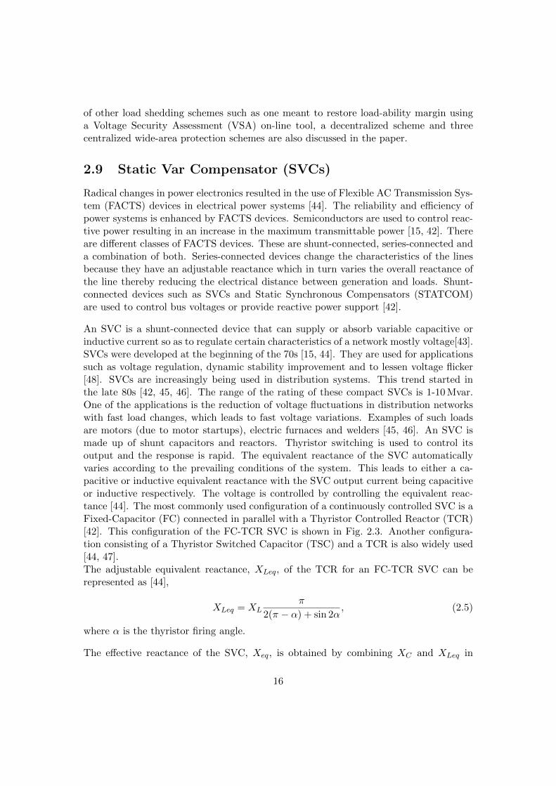
Radical changes in power electronics resulted in the use of Flexible AC Transmission Sys-tem (FACTS) devices in electrical power systems [44]. The reliability and efficiency ofpower systems is enhanced by FACTS devices. Semiconductors are used to control reac-tive power resulting in an increase in the maximum transmittable power [15, 42]. Thereare different classes of FACTS devices. These are shunt-connected, series-connected anda combination of both. Series-connected devices change the characteristics of the linesbecause they have an adjustable reactance which in turn varies the overall reactance ofthe line thereby reducing the electrical distance between generation and loads. Shunt-connected devices such as SVCs and Static Synchronous Compensators (STATCOM)are used to control bus voltages or provide reactive power support [42].

An SVC is a shunt-connected device that can supply or absorb variable capacitive orinductive current so as to regulate certain characteristics of a network mostly voltage[43].SVCs were developed at the beginning of the 70s [15, 44]. They are used for applicationssuch as voltage regulation, dynamic stability improvement and to lessen voltage flicker[48]. SVCs are increasingly being used in distribution systems. This trend started inthe late 80s [42, 45, 46]. The range of the rating of these compact SVCs is 1-10 Mvar.One of the applications is the reduction of voltage fluctuations in distribution networkswith fast load changes, which leads to fast voltage variations. Examples of such loadsare motors (due to motor startups), electric furnaces and welders [45, 46]. An SVC ismade up of shunt capacitors and reactors. Thyristor switching is used to control itsoutput and the response is rapid. The equivalent reactance of the SVC automaticallyvaries according to the prevailing conditions of the system. This leads to either a ca-pacitive or inductive equivalent reactance with the SVC output current being capacitiveor inductive respectively. The voltage is controlled by controlling the equivalent reac-tance [44]. The most commonly used configuration of a continuously controlled SVC is aFixed-Capacitor (FC) connected in parallel with a Thyristor Controlled Reactor (TCR)[42]. This configuration of the FC-TCR SVC is shown in Fig. 2.3. Another configura-tion consisting of a Thyristor Switched Capacitor (TSC) and a TCR is also widely used[44, 47].The adjustable equivalent reactance, XLeq, of the TCR for an FC-TCR SVC can berepresented as [44],

XLeq = XLπ

2(π − α) + sin 2α, (2.5)

where α is the thyristor firing angle.

The effective reactance of the SVC, Xeq, is obtained by combining XC and XLeq in

16

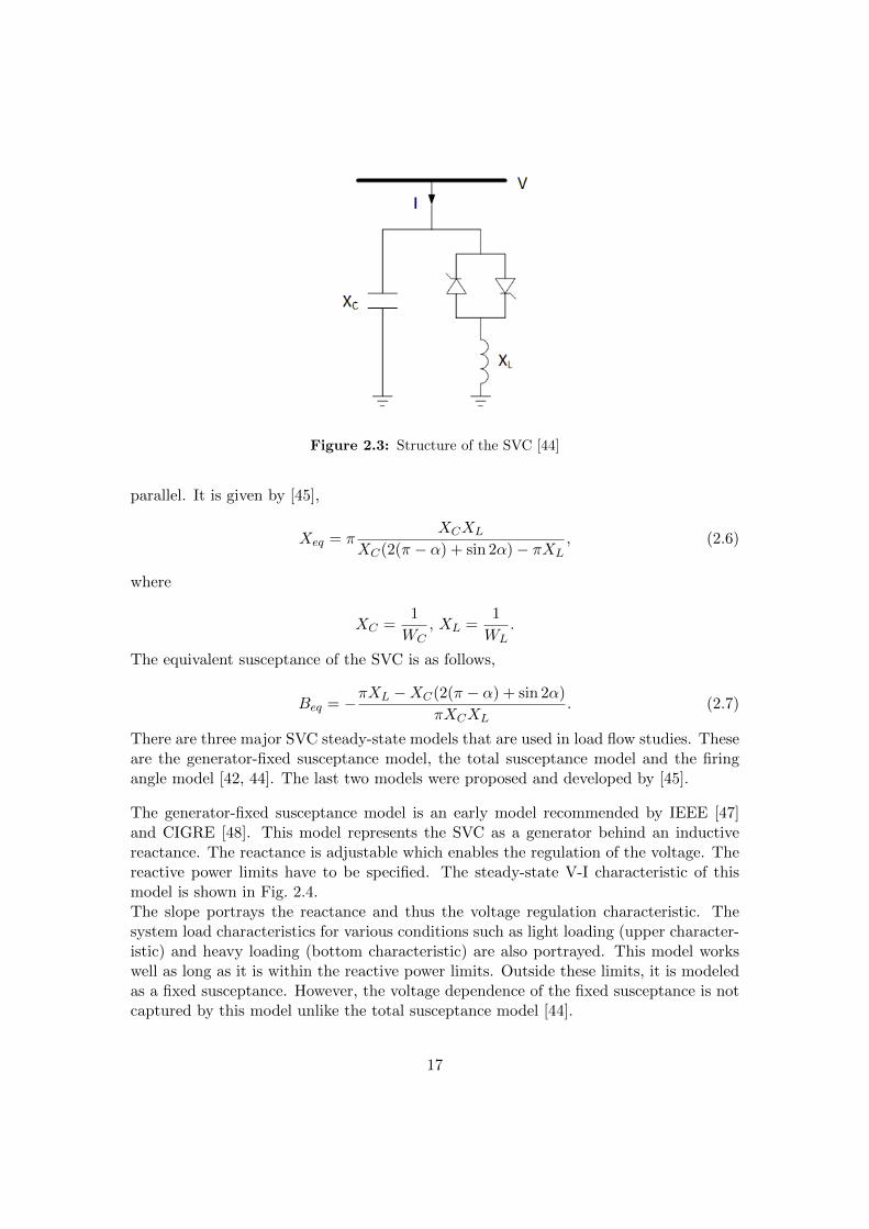
Figure 2.3: Structure of the SVC [44]

parallel. It is given by [45],

Xeq = πXCXL

XC(2(π − α) + sin 2α)− πXL, (2.6)

where

XC =1

WC, XL =

1

WL.

The equivalent susceptance of the SVC is as follows,

Beq = −πXL −XC(2(π − α) + sin 2α)

πXCXL. (2.7)

There are three major SVC steady-state models that are used in load flow studies. Theseare the generator-fixed susceptance model, the total susceptance model and the firingangle model [42, 44]. The last two models were proposed and developed by [45].

The generator-fixed susceptance model is an early model recommended by IEEE [47]and CIGRE [48]. This model represents the SVC as a generator behind an inductivereactance. The reactance is adjustable which enables the regulation of the voltage. Thereactive power limits have to be specified. The steady-state V-I characteristic of thismodel is shown in Fig. 2.4.The slope portrays the reactance and thus the voltage regulation characteristic. Thesystem load characteristics for various conditions such as light loading (upper character-istic) and heavy loading (bottom characteristic) are also portrayed. This model workswell as long as it is within the reactive power limits. Outside these limits, it is modeledas a fixed susceptance. However, the voltage dependence of the fixed susceptance is notcaptured by this model unlike the total susceptance model [44].

17

In the total susceptance model, the SVC is portrayed as a variable susceptance as shownin Fig. 2.5. Limits are applied to the susceptance to represent the rating [42, 44].From Fig. 2.5, the current in the SVC and reactive power are, respectively, [44]

I = jBVk, (2.8)

Qk = −V 2k B. (2.9)

The linearized equation of the SVC can also be obtained from Fig. 2.5 and is expressedas [44], [

∆Pk

∆Qk

]=

[0 0

0 Qk

]×

[∆δk

∆Bsvc/Bsvc

]. (2.10)

This equation, with susceptance taken as the state variable is needed for the Newton-Raphson power flow. The value of the susceptance is found using an iterative processwhich is given by [44]

Bi+1SV C = Bi

SV C + (∆BSV C/BSV C)BiSV C . (2.11)

The susceptance changes according to the compensation that is required. The totalsusceptance that is found is the one that is needed to sustain the voltage at the desiredlevel. This susceptance is then used to determine the firing angle. This is also done byiteration.

In the firing angle model, the equivalent susceptance of the SVC depends on the firingangle, α, of the thyristors and the representation is as shown in Fig. 2.4. The modelis portrayed by a thyristor controlled reactor in parallel with a fixed capacitor. Thelinearized SVC equation is expressed as [44],[

∆Pk

∆Qk

]=

[0 0

0 ∂Qk∂α

]×

[∆δk

∆α

], (2.12)

Figure 2.4: SVC steady-state V-I characteristic [44].

18

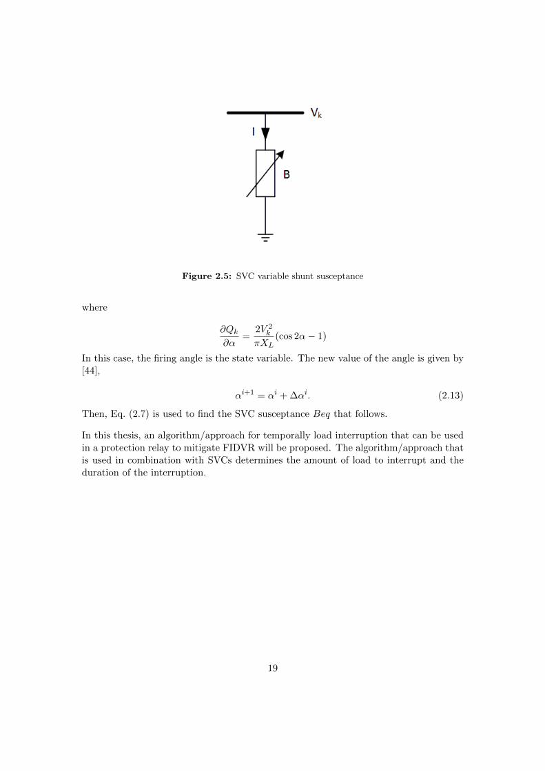
Figure 2.5: SVC variable shunt susceptance

where

∂Qk∂α

=2V 2

k

πXL(cos 2α− 1)

In this case, the firing angle is the state variable. The new value of the angle is given by[44],

αi+1 = αi + ∆αi. (2.13)

Then, Eq. (2.7) is used to find the SVC susceptance Beq that follows.

In this thesis, an algorithm/approach for temporally load interruption that can be usedin a protection relay to mitigate FIDVR will be proposed. The algorithm/approach thatis used in combination with SVCs determines the amount of load to interrupt and theduration of the interruption.

19

3Induction Motor Model

Due to the fact that this thesis is dealing with induction machines, the purpose ofthe present chapter is to provide to the reader a simple introduction to them.For it to be a complete treatment, the main goal is to explain the behavior ofinduction machines and the manner in which they can be exclusively modeled

using PSS/E.

The first part of the chapter is devoted to defining an induction motor by describing itscomponents, explaining the physical principles that govern its functioning and, by settingthe set of mathematical expressions that model the system. The second part introducesthe modeling of induction motors in PSS/E. The problems faced during the simulationprocess are highlighted and described. Similarly, the solution to those problems are verywell documented. It is hoped that the material included in the thesis can serve as auseful guide for future users of PSS/E.

3.1 Induction motor

An AC induction motor is an electromechanical system that converts electrical energyinto mechanical one. The main feature of an induction motor is the mechanism by whichthe electric current in the rotor is generated. For an AC electric motor the current onthe rotor is generated by electromagnetic induction, in this case, from the magnetic fieldof the stator winding. As a consequence, an induction machine does not require anykind of mechanical commutation, separate-excitation or self-excitation for all or part ofthe energy transferred from the stator to the rotor. This is one of the major differenceswhen compared to dc electrical machines.

In the above framework, the physical principle that leads to the functioning of an ACmachine is the Induction law of Faraday. In this case, an external AC current is suppliedto the stator, but no external DC field current is provided to the rotor. The resulting

20

AC currents in the rotor are the result of electromagnetic induction [49], [50] [51].

In this section, the protocols and procedures for setting up simulations of inductionmachines in PSS/E are described in detail. The document is mainly based from theexperience acquired from the authors during the completion of the thesis and fromSiemens Power Technologies International’s (PTI) program manuals.

There are two ways of modeling induction machines in PSS/E. The first one consists ofconnecting the induction machine directly to the bus through an induction machine icon.In this case, at least one induction machine data record must be specified at each networkbus at which an induction machine is to be represented. Multiple induction machinesmay be represented at a bus by specifying more than one induction machine data recordfor the bus, each with a different machine identifier. It is important to highlight thatthe induction machine simulation icons are available in version 33.4 and 33.5. Thesecond one consists of representing the induction machine as a bus load in the load flowsimulation and incorporating this load into one of the pre-defined load models availablein PSS/E for dynamic simulations (see descriptions of the models below). During theexecution of this thesis the second way was chosen due to initialization problems in theload flow studies and the lack of load models for dynamic simulations with the first way.Independent of the choice, the results coming from both ways should provide the smallresults. The following paragraphs are devoted to analyzing the simulation process usingthe second method.

3.2 Simulation process of an induction motor as a bus loadin PSS/E

As one of the main purposes of this thesis was to implement the model used by ProfessorCutsem, see [5], the initial step of this work was to determine the kind of model that bestfits the physical behavior of this system within PSS/E. After discussion with ProfessorCutsem, and due to the characteristics of the system: rotating load dynamics, it wasdetermined that the induction motor load in the system can be classified under theumbrella of the CIM5BL model, double cage type 1 motor in PSS/E. The purpose ofthe following paragraphs is to explain this terminology and clarify the way of reasoningthat led the authors to this assertion.

3.3 Equivalent circuit

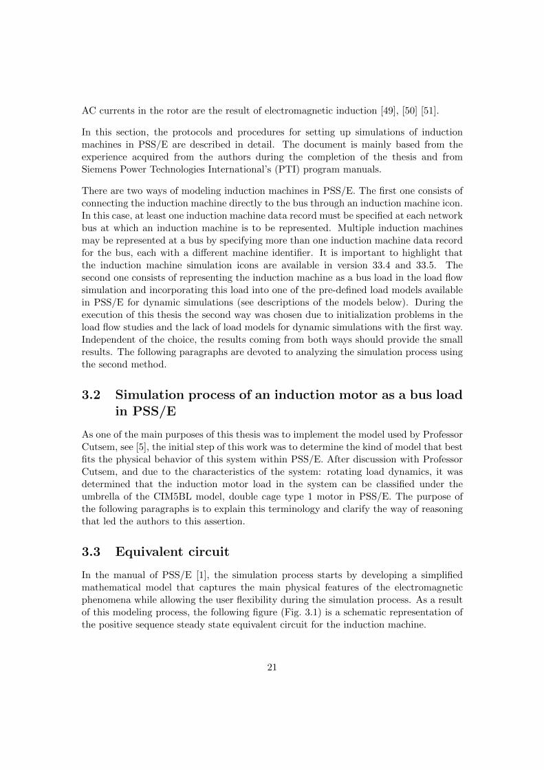
In the manual of PSS/E [1], the simulation process starts by developing a simplifiedmathematical model that captures the main physical features of the electromagneticphenomena while allowing the user flexibility during the simulation process. As a resultof this modeling process, the following figure (Fig. 3.1) is a schematic representation ofthe positive sequence steady state equivalent circuit for the induction machine.

21

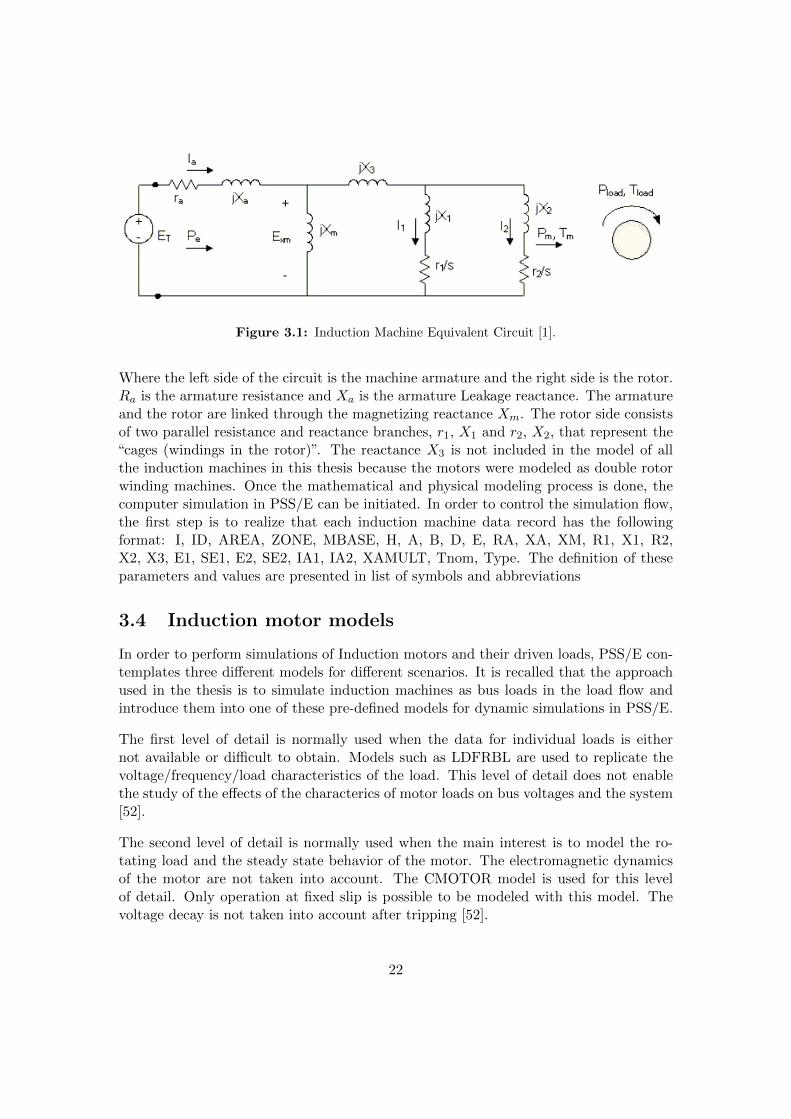
Figure 3.1: Induction Machine Equivalent Circuit [1].

Where the left side of the circuit is the machine armature and the right side is the rotor.Ra is the armature resistance and Xa is the armature Leakage reactance. The armatureand the rotor are linked through the magnetizing reactance Xm. The rotor side consistsof two parallel resistance and reactance branches, r1, X1 and r2, X2, that represent the“cages (windings in the rotor)”. The reactance X3 is not included in the model of allthe induction machines in this thesis because the motors were modeled as double rotorwinding machines. Once the mathematical and physical modeling process is done, thecomputer simulation in PSS/E can be initiated. In order to control the simulation flow,the first step is to realize that each induction machine data record has the followingformat: I, ID, AREA, ZONE, MBASE, H, A, B, D, E, RA, XA, XM, R1, X1, R2,X2, X3, E1, SE1, E2, SE2, IA1, IA2, XAMULT, Tnom, Type. The definition of theseparameters and values are presented in list of symbols and abbreviations

3.4 Induction motor models

In order to perform simulations of Induction motors and their driven loads, PSS/E con-templates three different models for different scenarios. It is recalled that the approachused in the thesis is to simulate induction machines as bus loads in the load flow andintroduce them into one of these pre-defined models for dynamic simulations in PSS/E.

The first level of detail is normally used when the data for individual loads is eithernot available or difficult to obtain. Models such as LDFRBL are used to replicate thevoltage/frequency/load characteristics of the load. This level of detail does not enablethe study of the effects of the characterics of motor loads on bus voltages and the system[52].

The second level of detail is normally used when the main interest is to model the ro-tating load and the steady state behavior of the motor. The electromagnetic dynamicsof the motor are not taken into account. The CMOTOR model is used for this levelof detail. Only operation at fixed slip is possible to be modeled with this model. Thevoltage decay is not taken into account after tripping [52].

22

The third level of detail takes into account the motor electromagnetic dynamics and ro-tating load dynamics. These are thoroughly represented at this level. The models thatare used for this level are the CIM5BL, CIM6BL, CIMWBL, CIMTR2 and CIMTR4.CIM5BL has been selected because it best suits the network that is being studied. Inthis level of detail, the transient component starts from zero but responds to changes inthe network conditions such as voltage to reflect rotor flux linkages. The transient andsub-transient time constants of the rotor winding determine the decay.

From the above description, due to the fact that the modeling of an induction machinewith rotating loads is of primary interest, it is concluded that the model studied by [5]can be classified by approach number 3. What is remaining now, is to determine thespecific model and the type of motor to which it belongs. These questions will be thetopic of discussion for the next sections.

3.5 Induction Motor Load Model CIM5BL

The CIM5BL model can be used to model either single-cage or double-cage inductionmotors including rotor flux dynamics. In addition, the effects of rotating load dynamicscan be included. These features makes it a promising candidate to the studied system[5] .

In the power flow, the motor is modeled as a bus load where the entire load at a specificload ID is taken as constant power load. These models may be applied to an individualload or a subsystem of loads. The data input for the model are the equivalent circuitimpedances for Type 1 equivalent circuit model. These can be seen in Fig. 3.2. TheModel Type is specified in ICON(M+1).

Figure 3.2: CIM5 Type Model [1].

The CIM5 models translate the equivalent circuit parameters into transient parameters(flux linkage components) for use in the actual model calculations, according to theequations in Fig. 3.3.

The equivalent circuit impedances are specified in per unit on motor MVA base. Theuser has two choices for the specification of motor MVA base:

23

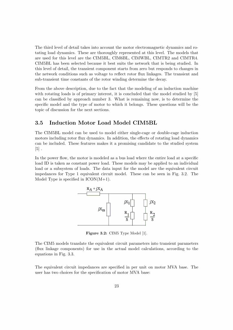
CONs Description

J RA

J +1 XA

J+2 Xm>0 ICON Description

J+3 R1 M IT, motor type (1 or 2)

J+4 X1 >0

J+5 R2 (0 for single cage)1"

J+6 X2 (0 for single cage)

J+7 E1 >= 0

J+8 S(E1) VARs Description

J+9 E2 L Admittance of initial condition Mvar difference

J+10 S(E2) L+1 Motor Q

J+11 MBASE 2" L+2 Telec (pu motor base)

J+12 PMULT L+3 T (pu on motor base)1, 2

J+13 H (inertia, per unit motor base) L+4 IQ

J+14 VI (pu) 3" L+5 ID

J+15 TI (cycles) 4" L+6 Motor current (pu motor base)

J+16 TB (cycles) L+7 Relay trip time

J+17 D (load damping factor) L+8 Breaker trip time

J+18Tnom, Load torque at 1 pu speed (used for motor starting

only) >= 0)L+9 MVA rating

2 For motor starting, T=Tnom is specified by the user in CON (J+18).

For motor online studies, T=To is calculated in the code during

initialization and stored in VAR (L+4).

1 Load torque, TL = T (1 + D33)D 1 To model single cage motor: set R2 = X2 = 0.

2 When MBASE = 0, motor MVA base = PMULT x MW load. When

MBASE > 0, motor MVA base = MBASE.

3 VI is the per unit voltage level below which the relay to trip the

motor will begin timing. To disable relay, set VI = 0.

4 TI is the time in cycles for which the voltage must remain below the

threshold for the relay to trip. TB is the breaker delay time cycles

Figure 3.3: Induction Motor Load Model CIM5BL[53]. Model of CIM5BL general descrip-tion.

1. When CON(J+11) > 0., the motor MVA base is specified as CON(J+11).

2. When CON(J+11) = 0., the motor MVA base is specified as CON(J+12)*MWload.

3.6 IMD application tool

During the simulation process, one major problem that was faced was to determine theappropriate nominal torque Tnom. During the course of this thesis the values for allthe parameters of the machine were tested in the (IMD) application tool from PSS/Eutilities. Tnom was determined (and specified in CON(J+18) from motor data. Tnomwas calculated through motor parameters (IMD) tool. It is important to mention thatthe motor nominal rating was used to specify MVA base in CON(J+11), MBASE. Inaddition, the simulation integration time step should be reduced in order to preventinstability of the system during dynamic simulations.

24

3.7 Motor type 1

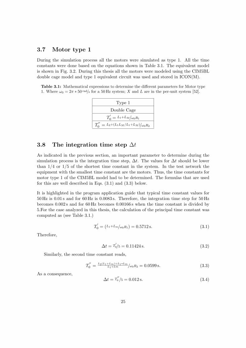
During the simulation process all the motors were simulated as type 1. All the timeconstants were done based on the equations shown in Table 3.1. The equivalent modelis shown in Fig. 3.2. During this thesis all the motors were modeled using the CIM5BLdouble cage model and type 1 equivalent circuit was used and stored in ICON(M).

Table 3.1: Mathematical expressions to determine the different parameters for Motor type1. Where ω0 = 2π ∗ 50 rad/s for a 50 Hz system; X and L are in the per-unit system [52].

Type 1

Double Cage

T′0 = L1+LM/ω0R1

T′′0 = L2+(L1LM/L1+LM )/ω0R2

3.8 The integration time step ∆t

As indicated in the previous section, an important parameter to determine during thesimulation process is the integration time step, ∆t. The values for ∆t should be lowerthan 1/4 or 1/5 of the shortest time constant in the system. In the test network theequipment with the smallest time constant are the motors. Thus, the time constants formotor type 1 of the CIM5BL model had to be determined. The formulas that are usedfor this are well described in Eqs. (3.1) and (3.3) below.

It is highlighted in the program application guide that typical time constant values for50 Hz is 0.01 s and for 60 Hz is 0.0083 s. Therefore, the integration time step for 50 Hzbecomes 0.002 s and for 60 Hz becomes 0.00166 s when the time constant is divided by5.For the case analyzed in this thesis, the calculation of the principal time constant wascomputed as (see Table 3.1.)

T′0 = (L1+Lm/ω0R1) = 0.5712 s. (3.1)

Therefore,

∆t = T′0/5 = 0.11424 s. (3.2)

Similarly, the second time constant reads,

T′′0 =

L2(L1+Lm)+L1∗LmL1+Lm /ω0R2 = 0.0599 s. (3.3)

As a consequence,∆t = T

′′0 /5 = 0.012 s. (3.4)

25

4Load flow and dynamic simulation

using PSS/E

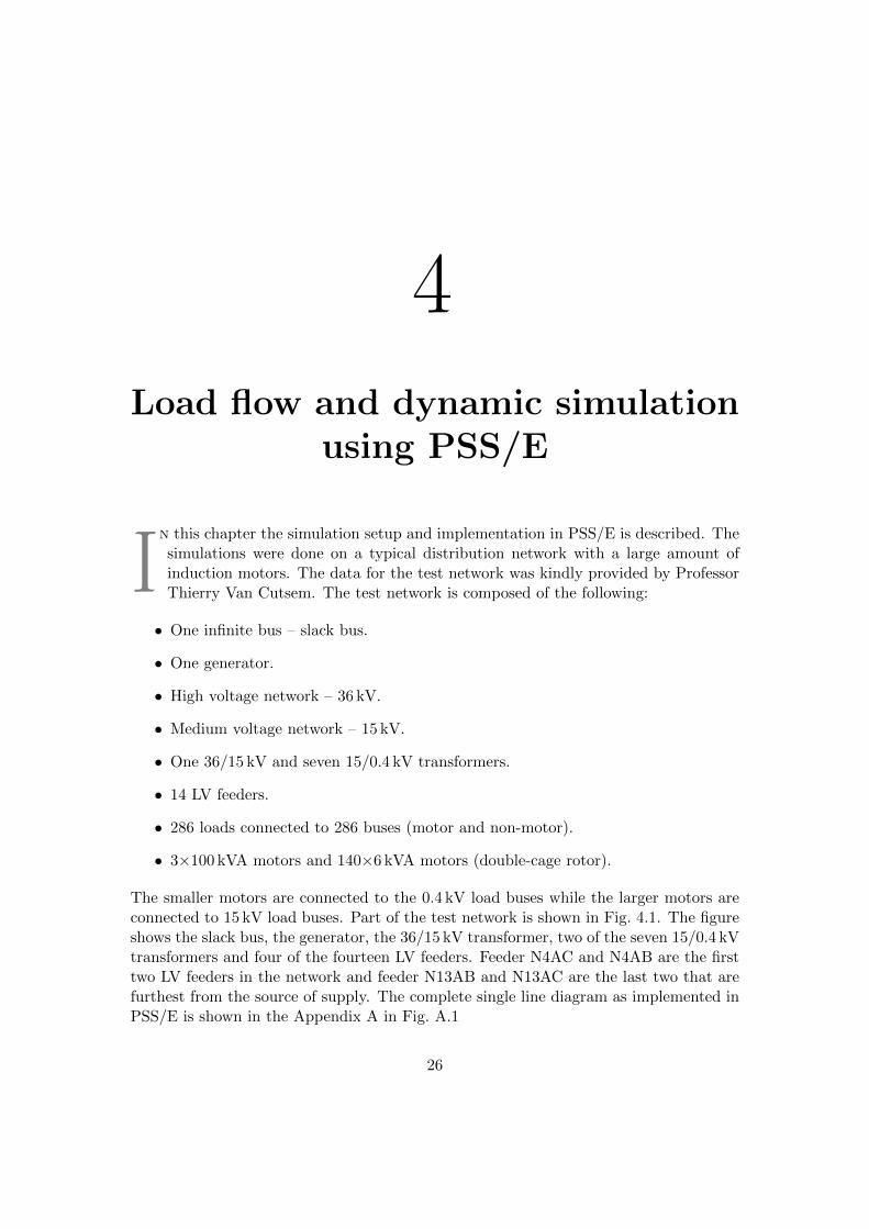
In this chapter the simulation setup and implementation in PSS/E is described. Thesimulations were done on a typical distribution network with a large amount ofinduction motors. The data for the test network was kindly provided by ProfessorThierry Van Cutsem. The test network is composed of the following:

• One infinite bus – slack bus.

• One generator.

• High voltage network – 36 kV.

• Medium voltage network – 15 kV.

• One 36/15 kV and seven 15/0.4 kV transformers.

• 14 LV feeders.

• 286 loads connected to 286 buses (motor and non-motor).

• 3×100 kVA motors and 140×6 kVA motors (double-cage rotor).

The smaller motors are connected to the 0.4 kV load buses while the larger motors areconnected to 15 kV load buses. Part of the test network is shown in Fig. 4.1. The figureshows the slack bus, the generator, the 36/15 kV transformer, two of the seven 15/0.4 kVtransformers and four of the fourteen LV feeders. Feeder N4AC and N4AB are the firsttwo LV feeders in the network and feeder N13AB and N13AC are the last two that arefurthest from the source of supply. The complete single line diagram as implemented inPSS/E is shown in the Appendix A in Fig. A.1

26

Figure 4.1: Single line diagram showing part of the test system [5].

4.1 Directories and Files Overview

During the simulation process a folder with an unlimited number of files was created forPSS/E. Two subfolders were created one for load flow and the second one for dynamicsimulations. It is important to mention that PSS/E always runs out of a working folder[1]. PSS/E uses two types of files, input files and output files. These types of files canbe seen by PSS/E as:

1. Input files. Data required by PSS/E. All the files are created by the user.

2. Output files. This type of file includes results and files generated automatically byPSS/E.

PSS/E uses three different types of files. These are source, binary and both source andbinary. Source files can be used by PSS/E and the user. Binary files are used by PSS/E.Source and Binary can be used by PSS/E and other programs [1].

File formats used during the load flow and dynamic simulations are:

1. Slider diagram file (.sld). Containing all the data for the line diagram and it islinked with save case file.

27

2. Save case file (.sav). Binary file containing the power flow data, [1].

3. Power flow data file (.raw). Containing the power flow data for the initial workingcase [1]

4. Dynamic data file (.dyr). File containing all the machine data necessary to performdynamic simulations, [1].

5. Snapshot file (.snp). Binary file containing all the data at an exact instant duringdynamic state.

6. Output file (.out). File containing all the information saved after the dynamicsimulation.

4.2 Steady-state load flow

The parameters used to run the load flow simulation during this thesis are also the onesthat were used in [5]. However, the fraction of motor load used in this thesis is 50%while 60% was used in [5]. All the loads were modeled as constant power loads in theload flow analysis. Full Newton-Raphson method was used for the load flow solutionin this thesis. For load flow simulation all the parameters of the transmission lines andtransformers used are in pu. The parameters were obtained as shown below

ZBase =V 2Base

SBase, (4.1)

Zpu =ZrealZBase

, (4.2)

Xnewpu = Xold

pu ×V 2old

Sold×SnewBase

V 2newBase

. (4.3)

From the above equations, line and transformer parameters are calculated.

In PSS/E load flow simulation can be performed as follows:

1. In the toolbar click new.

2. Network case and diagram.

3. Build new case.

4. Draw the diagram with the aid of the toolbar. Use the load icon to represent thestatic and induction machine loads. Therefore, two load icons are connected toeach load bus. The induction machine icon is not used in this project.

5. Enter all the parameters of the machines (total machine load for each bus), buses,branches and transformers.

28

6. Save in the format of (.sav and .sld).

Below is an explanation of how to run the load flow:

1. On the toolbar click Power flow.

2. Followed by solution.

3. Then click solve (NSOL/FNSL/FDNS/SOLV/MSLV).

4. In the window displayed (load flow solutions) select the type of solution required.Full Newton-Rhpason (FNSL) was used in this thesis.

5. Click Solve.

6. Then Close.

4.3 Dynamic simulation connection of the induction ma-chines (IMD)

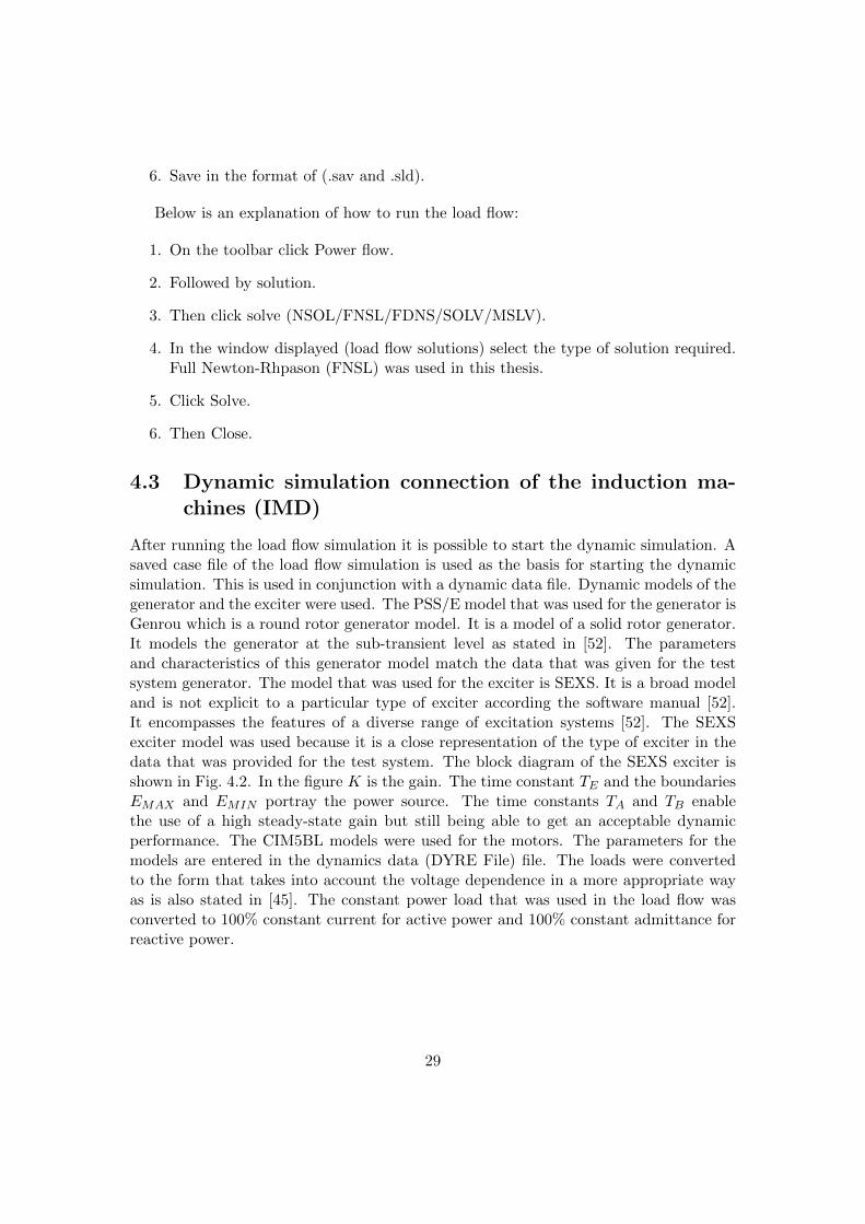
After running the load flow simulation it is possible to start the dynamic simulation. Asaved case file of the load flow simulation is used as the basis for starting the dynamicsimulation. This is used in conjunction with a dynamic data file. Dynamic models of thegenerator and the exciter were used. The PSS/E model that was used for the generator isGenrou which is a round rotor generator model. It is a model of a solid rotor generator.It models the generator at the sub-transient level as stated in [52]. The parametersand characteristics of this generator model match the data that was given for the testsystem generator. The model that was used for the exciter is SEXS. It is a broad modeland is not explicit to a particular type of exciter according the software manual [52].It encompasses the features of a diverse range of excitation systems [52]. The SEXSexciter model was used because it is a close representation of the type of exciter in thedata that was provided for the test system. The block diagram of the SEXS exciter isshown in Fig. 4.2. In the figure K is the gain. The time constant TE and the boundariesEMAX and EMIN portray the power source. The time constants TA and TB enablethe use of a high steady-state gain but still being able to get an acceptable dynamicperformance. The CIM5BL models were used for the motors. The parameters for themodels are entered in the dynamics data (DYRE File) file. The loads were convertedto the form that takes into account the voltage dependence in a more appropriate wayas is also stated in [45]. The constant power load that was used in the load flow wasconverted to 100% constant current for active power and 100% constant admittance forreactive power.

29

∑

EMIN

EMAX

EFD

VS

+

VREF

+

-EC

(pu)

VS = VOTHSG + VUEL + VOEL

Figure 4.2: Generator exciter model block diagram [53].

The simulation setup for running dynamic simulations can be performed as follows:

1. Open the .sav and .sld files previously created in the power flow

2. Run the load flow.

3. Connect an extra load to each bus in order to simulate it as an IMD.

4. In toolbar click view.

5. Click dynamic tree view.

6. Click device models then machines and click on one of the machines.

7. Dynamic data will be displayed.

8. Insert machine parameters. For this simulation GENROU model was selected forthe generators since the generators are for a thermal power station.

9. For this simulation the exciter model that was selected is SEXS.

10. At the lower flange of the window click on Load Bus. This is done with the objectiveof connecting the induction machine models.

11. In Load Characteristc Model (double click to see the induction machine models oneach bus) CIM5BL was selected for all the buses. It is important to mention thatTnom was calculated from the PSS/E utility for motor parameters (IMD).

12. Save the dynamic data (.dyr) , (.raw) , (.snp) file format.

30

Below is an explanation of how to run dynamic simulations:

1. On toolbar click Power flow.

2. Then click convert loads and generators.

3. On the toolbar click power flow again and then click solution.

4. Then click order network for matrix operations (ORDR). Assume all the branchesare in service was selected on the window that pops up.

5. Then click power flow/solution then factorize admittance matrix (FACT)

6. Then click power flow/solution then solution for switching studies. Select usevoltage vector as start point and select factorize before performing solution (FACT)checkbox before clicking ok.

7. On the toolbar click Dynamics

8. Click on channel setup wizard and then select the check-boxes for the quantitiesthat you want to be included in the output such as voltage, speed, flow (P & Q),etc.

9. Click finish in the channel setup wizard.

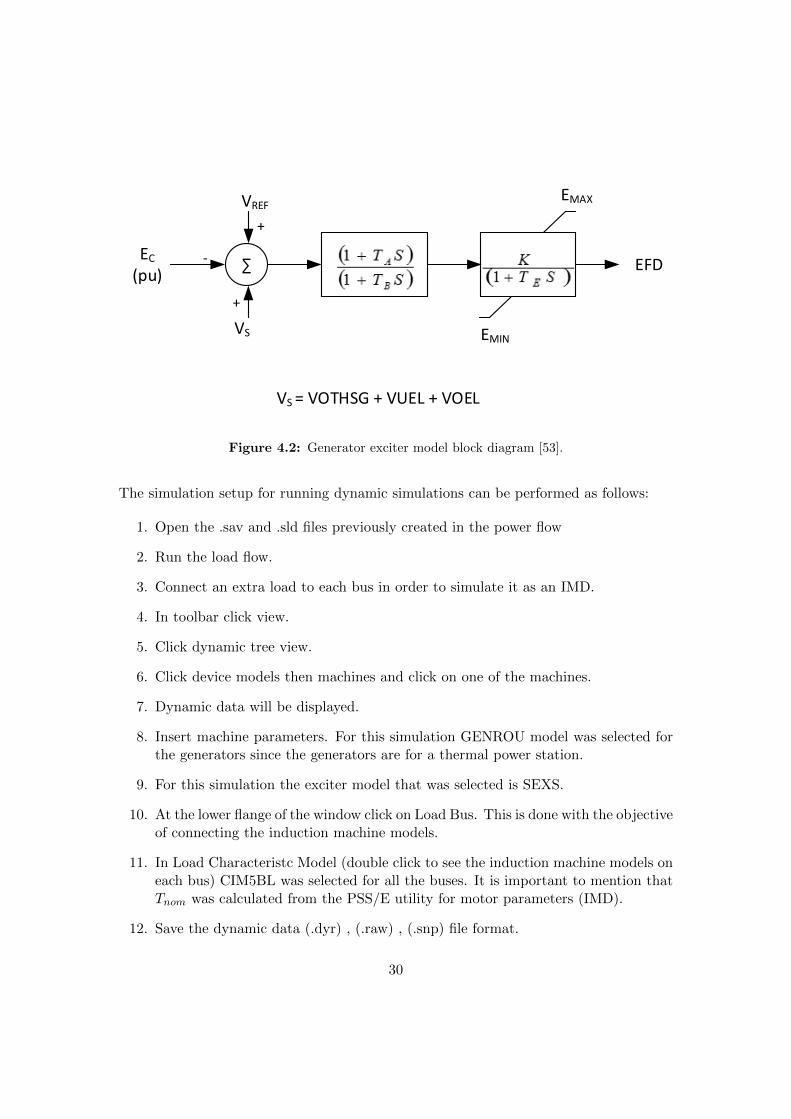
10. On the toolbar click Dynamics. Click on solution parameters and enter the inte-gration time step, DELT. The integration time step ∆t was calculated in previousChapters. See Fig.4.3.

11. On the toolbar click on Dynamics.

12. Click on simulation and then click on perform simulation (STRT/RUN).

13. In the perform dynamic simulation window specify a name for the channel outputfile (.out)

14. Click on Initialize.

15. Run for a certain period of time (pre-disturbance time) for instance a time of 1 s.

16. On the toolbar click on disturbance.

17. Create a disturbance by selecting the element where the fault will be applied.Afault was applied on one of the circuits between bus Node 1 and Node 2 for thiscase.

18. And run for a certain period of time such as 0.2 s.

19. Click on disturbance/clear fault.

31

Figure 4.3: Setting the integration time step in PSSE

20. Run for a certain period of time such as 1 or 2 seconds.

21. Click on close.

22. On the toolbar click open.

23. Open the OUT. File that was saved previously.

24. The graphics of the results for the dynamic simulations can then be analyzed.

4.4 Python programming language

Python was used in this thesis to control PSS/E. Python is a generic programminglanguage which is extensively in use [54]. It is an interpreted language. It is one of theprogram automation processors used to control PSS/E. Any type of program can also bewritten using python [1]. The Application Program Interface (API) was used to accessPSS/E functionality. The psspy python extension module was used to access the API.Python syntax was used when doing simulation runs for load interruption. It was usedfor load flow, dynamic simulations, tripping loads and then reconnecting them in stepsto automate the process. It was also used to automate the dynamic simulations forvoltage stability improvement using SVCs. Dynamic simulations with the undervoltageload shedding relay were also automated using python. The methodology that was usedfor the various simulation cases is illustrated in Fig. 4.4.

32

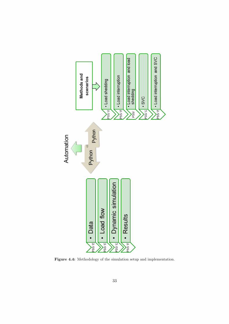
Figure 4.4: Methodology of the simulation setup and implementation.

33

5Improvement of voltage stabilityby temporary load interruption

In this chapter, different scenarios of improving voltage stability by the load inter-ruption method which was introduced in [5] are simulated. Simulations have beendone in PSS/E on a test network of a typical distribution system that has a largeshare of motor loads. Python was used to run and control PSS/E. The Python

syntax in the API was used. The simulation was therefore automated. However, therecovery of the voltage had to be checked after every simulation run and then more loadearmarked for interruption and included in the Python script until the desired outcomeis obtained. There is currently no API Python syntax for PSS/E to directly interrupt theload that is to trip and then reconnect the load at a bus. The only means to trip the loadis through the Under-voltage Load Shedding (LVSH type) relay model or by creating auser written model. However, the LVSH relay model only trips the load when the voltageis below a given threshold but it does not reconnect the load. Creating a user writtenmodel would have also meant a different programming language (Fortran). Therefore,two additional buses were created and connected to each load bus via zero impedancelines. The non-motor load was connected to one of the new buses and the motor loadwas connected to the other bus. This arrangement can be seen in the Appendix A inFig. A.1. This is essentially the same as splitting the bus which is done by activity split(Activity SPLT) in PSSE. Initially, the simulation was run in steady state within theacceptable voltage range of 0.9 pu to 1.1 pu. The dynamic simulation was then initializedwith the pre-disturbance steady state normal conditions. The dynamic simulation wasrun with these conditions for 1 second. Thereafter, a three phase fault was applied onone of the lines between Node 1 and Node 2 in order to create a disturbance. The faultwas applied for 200 ms (10 cycles). According to the criteria that has been used in thisthesis, the voltage should recover to 0.9 pu within 1 s following a disturbance. This isthe criteria that was used in [5] were the network data was obtained. This criteria is

34

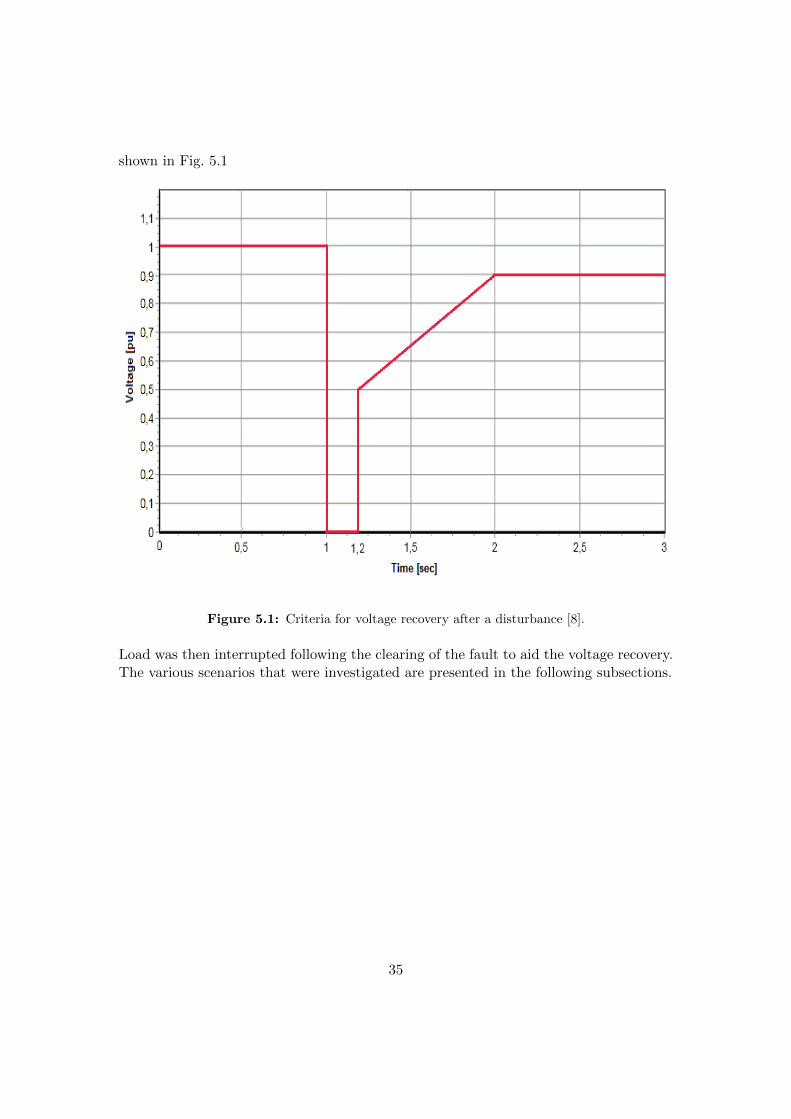
shown in Fig. 5.1

Figure 5.1: Criteria for voltage recovery after a disturbance [8].

Load was then interrupted following the clearing of the fault to aid the voltage recovery.The various scenarios that were investigated are presented in the following subsections.

35

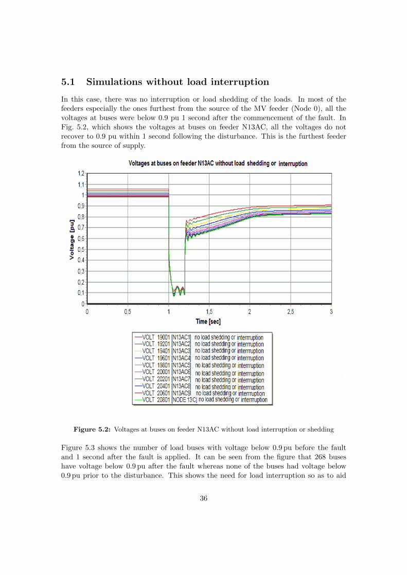
5.1 Simulations without load interruption

In this case, there was no interruption or load shedding of the loads. In most of thefeeders especially the ones furthest from the source of the MV feeder (Node 0), all thevoltages at buses were below 0.9 pu 1 second after the commencement of the fault. InFig. 5.2, which shows the voltages at buses on feeder N13AC, all the voltages do notrecover to 0.9 pu within 1 second following the disturbance. This is the furthest feederfrom the source of supply.

Figure 5.2: Voltages at buses on feeder N13AC without load interruption or shedding

Figure 5.3 shows the number of load buses with voltage below 0.9 pu before the faultand 1 second after the fault is applied. It can be seen from the figure that 268 buseshave voltage below 0.9 pu after the fault whereas none of the buses had voltage below0.9 pu prior to the disturbance. This shows the need for load interruption so as to aid

36

Figure 5.3: Number of load buses with voltage below 0.9 p.u 1 second after the fault.

the voltage recovery after fault clearance. The total number of load buses is 286.

5.2 Load shedding of 40%, 60% and 80% of non-motor load

In this scenario, the recovery of the voltage for load shedding of 40%, 60% and 80% ofnon-motor load is simulated. From Fig. 5.4 and Fig. 5.5 it is clear that the voltages atthe buses recover faster as the amount of load that is shed is increased. For instance, inFig. 5.4, it can be seen that the voltages at the buses on feeder N13AC recover faster asthe percentage of load that is disconnected is increased. For load shedding of 80% of thenon-motor load the majority of the voltages at the load buses recover above 0.9 pu at 2 s(1 s after the initiation of the disturbance). It can also be observed from Fig. 5.5 thatthe voltage at Node 13C recovers faster as the percent of load that is shed is increased.Node 13C is the furthest bus from the source of supply in the system.According to Fig. 5.6, the number of buses with voltage below 0.9 pu at 2 s with loadshedding is significantly lower than the case without load shedding. It is important tomention that at furthest points on feeders N13AC, N13AB, N11AC N11AB (the furthestfeeders from the source) the voltage recovers faster due to the shedding than the casewithout load shedding but still the voltage on some load buses are not able to reach0.9 pu at 2 s even for load shedding of 80% of the load. It is also important to mentionthat although most of the voltages recover to 0.9 pu at 2 s, load shedding is not the bestoption due to the fact that several loads are off for a long period of time. This is aninconvenience to consumers and can also result in lost revenue. It is also a cost to thegrid company as customers would have to be paid for being off supply. For this reason,another improvement method has been simulated.

37

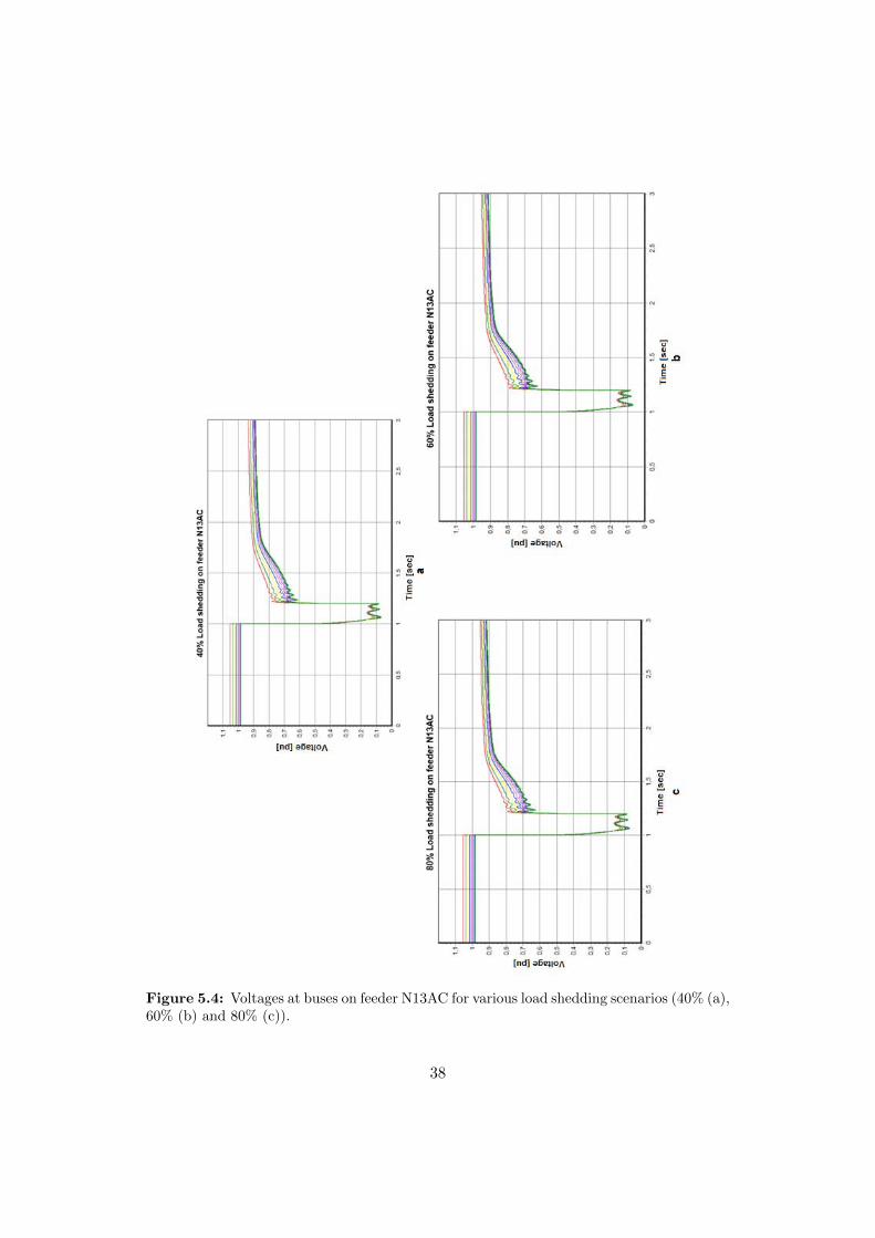
Figure 5.4: Voltages at buses on feeder N13AC for various load shedding scenarios (40% (a),60% (b) and 80% (c)).

38

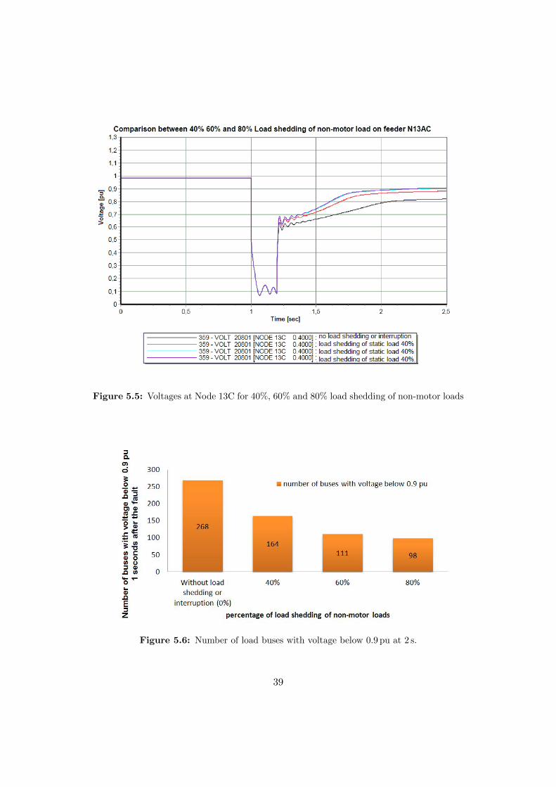
Figure 5.5: Voltages at Node 13C for 40%, 60% and 80% load shedding of non-motor loads

Figure 5.6: Number of load buses with voltage below 0.9 pu at 2 s.

39

5.3 Load shedding of various percentages of non-motor andmotor loads.

In this scenario, the recovery of the voltage to 0.9 pu 1 s after the disturbance with thedisconnection of non-motor and motor loads is studied. From an economical point ofview, it is important to say that the shedding of motor loads causes considerable ex-penses and further inconvenience for industries or customers who use a large share ofthe motors.

A considerable improvement in the recovery of voltages at buses in the system can beseen when non-motor and motor loads are disconnected. For instance, instead of having164 load buses with voltages below 0.9 pu at 2 s as is the case with 40% load shedding ofjust non-motor loads the simulations show that with load shedding of 40% of non-motorand 10% of motor loads the amount of load buses with voltage below 0.9 pu at 2 s reducesto 95. This can be seen by comparing Fig. 5.6 with Fig. 5.9.

The recovery of the voltage for the cases where load shedding of 40%, 50%, 60% and80% of non-motor loads is combined with shedding of motor loads was studied. Fourcases were investigated. These are the shedding of 10%, 20%, 40% and 80% of motorloads. Each of these four cases of shedding of motor loads was done together with loadshedding of 40%, 50%, 60% and 80% of non-motor loads. The results for the evolutionof the voltages are shown in Figs. 5.7, 5.10, 5.12, and 5.15. The voltages at Node 13Cfor the cases where 10% and 40% of motor load is shed are shown in Figs. 5.8 and 5.13,respectively. Figs. 5.9, 5.11, 5.14 and 5.16 show the number of buses with voltage below0.9 pu at 2 s. As can be seen from the figures, the higher the percentage of motor loadsthat are shed the faster the voltage recovers. In the case where a combination of shed-ding of 80% of non-motor and 80% of motor loads is studied, the number of buses withvoltage below 0.9 pu is only 26. However, as earlier stated the disadvantage with loadshedding is that the load is not saved. The load is just disconnected and not reconnectedso consumers remain off supply.

The results of the simulations for this specific case are shown below in the next subsec-tions.

40

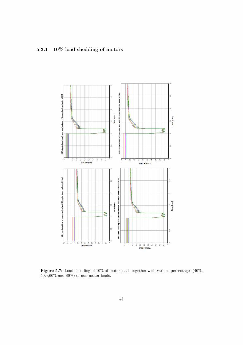
5.3.1 10% load shedding of motors

Figure 5.7: Load shedding of 10% of motor loads together with various percentages (40%,50%,60% and 80%) of non-motor loads.

41

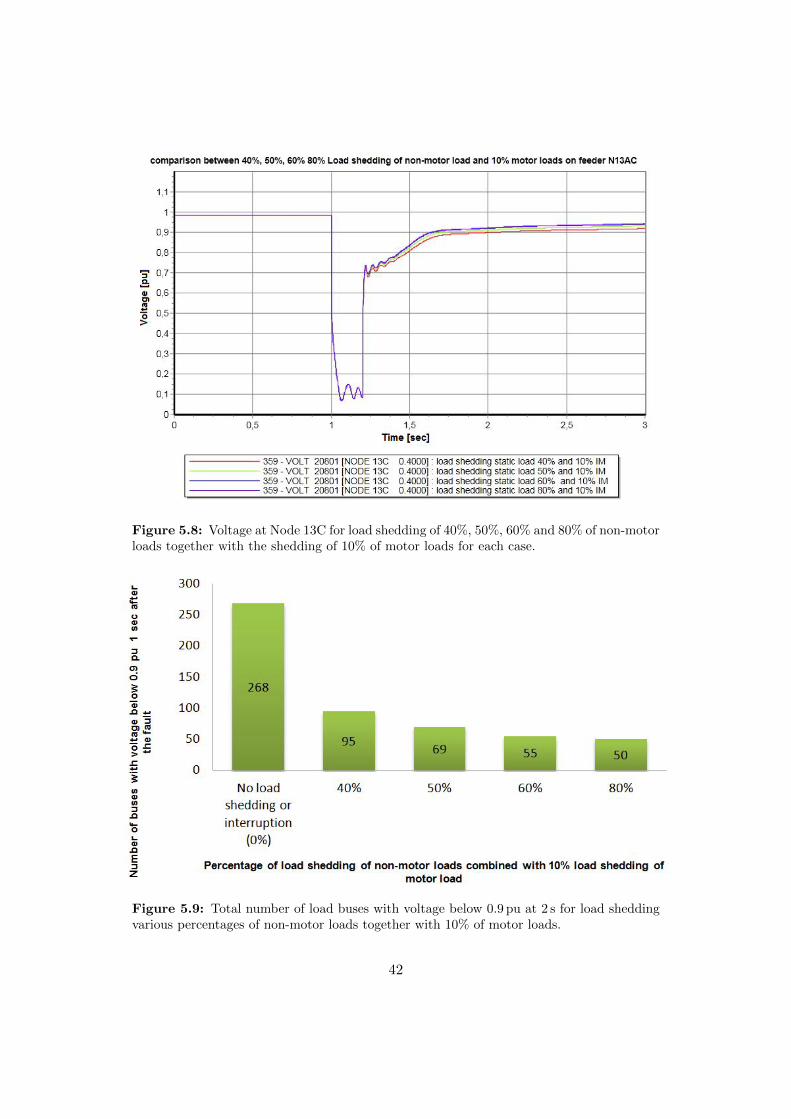
Figure 5.8: Voltage at Node 13C for load shedding of 40%, 50%, 60% and 80% of non-motorloads together with the shedding of 10% of motor loads for each case.

Figure 5.9: Total number of load buses with voltage below 0.9 pu at 2 s for load sheddingvarious percentages of non-motor loads together with 10% of motor loads.

42

5.3.2 20% load shedding of motors

Figure 5.10: Load shedding of 20% of motor loads together with various percentages (40%,50%, 60% and 80%) of non-motor loads.

43

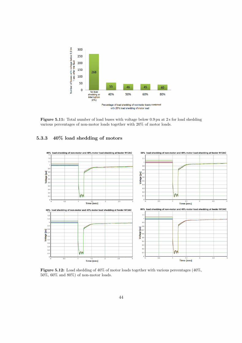
Figure 5.11: Total number of load buses with voltage below 0.9 pu at 2 s for load sheddingvarious percentages of non-motor loads together with 20% of motor loads.

5.3.3 40% load shedding of motors

Figure 5.12: Load shedding of 40% of motor loads together with various percentages (40%,50%, 60% and 80%) of non-motor loads.

44

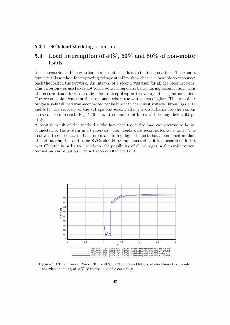
5.3.4 80% load shedding of motors

5.4 Load interruption of 40%, 60% and 80% of non-motorloads

In this scenario load interruption of non-motor loads is tested in simulations. The resultsfound in this method for improving voltage stability show that it is possible to reconnectback the load in the network. An interval of 1 second was used for all the reconnections.This criterion was used so as not to introduce a big disturbance during reconnection. Thisalso ensures that there is no big step or steep drop in the voltage during reconnection.The reconnection was first done at buses where the voltage was higher. This was doneprogressively till load was reconnected to the bus with the lowest voltage. From Figs. 5.17and 5.18, the recovery of the voltage one second after the disturbance for the variouscases can be observed. Fig. 5.19 shows the number of buses with voltage below 0.9 puat 2 s.A positive result of this method is the fact that the entire load can eventually be re-connected to the system in 1 s intervals. Four loads were reconnected at a time. Theload was therefore saved. It is important to highlight the fact that a combined methodof load interruption and using SVCs should be implemented as it has been done in thenext Chapter in order to investigate the possibility of all voltages in the entire systemrecovering above 0.9 pu within 1 second after the fault.

Figure 5.13: Voltage at Node 13C for 40%, 50%, 60% and 80% load shedding of non-motorloads with shedding of 40% of motor loads for each case.

45

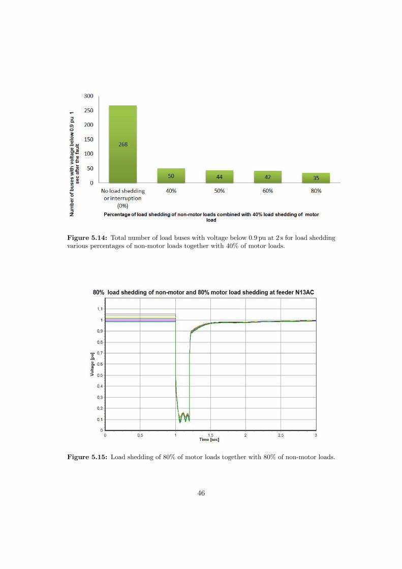
Figure 5.14: Total number of load buses with voltage below 0.9 pu at 2 s for load sheddingvarious percentages of non-motor loads together with 40% of motor loads.

Figure 5.15: Load shedding of 80% of motor loads together with 80% of non-motor loads.

46

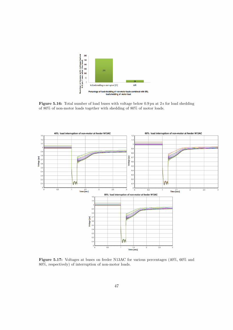
Figure 5.16: Total number of load buses with voltage below 0.9 pu at 2 s for load sheddingof 80% of non-motor loads together with shedding of 80% of motor loads.

Figure 5.17: Voltages at buses on feeder N13AC for various percentages (40%, 60% and80%, respectively) of interruption of non-motor loads.

47

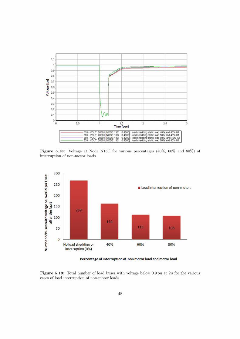
Figure 5.18: Voltage at Node N13C for various percentages (40%, 60% and 80%) ofinterruption of non-motor loads.

Figure 5.19: Total number of load buses with voltage below 0.9 pu at 2 s for the variouscases of load interruption of non-motor loads.

48

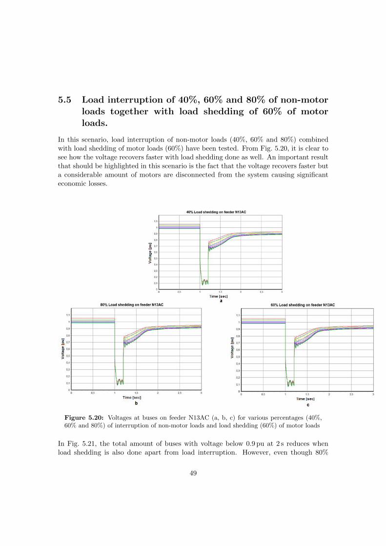
5.5 Load interruption of 40%, 60% and 80% of non-motorloads together with load shedding of 60% of motorloads.

In this scenario, load interruption of non-motor loads (40%, 60% and 80%) combinedwith load shedding of motor loads (60%) have been tested. From Fig. 5.20, it is clear tosee how the voltage recovers faster with load shedding done as well. An important resultthat should be highlighted in this scenario is the fact that the voltage recovers faster buta considerable amount of motors are disconnected from the system causing significanteconomic losses.

Figure 5.20: Voltages at buses on feeder N13AC (a, b, c) for various percentages (40%,60% and 80%) of interruption of non-motor loads and load shedding (60%) of motor loads

In Fig. 5.21, the total amount of buses with voltage below 0.9 pu at 2 s reduces whenload shedding is also done apart from load interruption. However, even though 80%

49

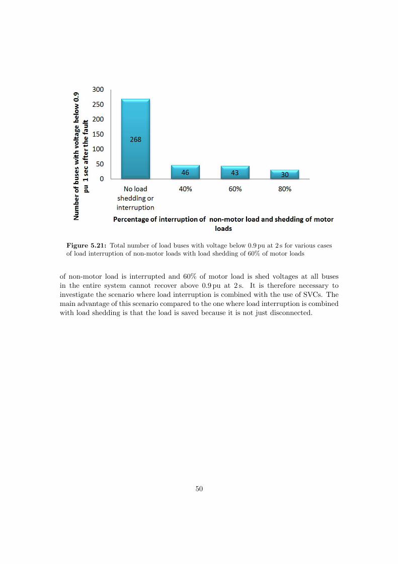
Figure 5.21: Total number of load buses with voltage below 0.9 pu at 2 s for various casesof load interruption of non-motor loads with load shedding of 60% of motor loads

of non-motor load is interrupted and 60% of motor load is shed voltages at all busesin the entire system cannot recover above 0.9 pu at 2 s. It is therefore necessary toinvestigate the scenario where load interruption is combined with the use of SVCs. Themain advantage of this scenario compared to the one where load interruption is combinedwith load shedding is that the load is saved because it is not just disconnected.

50

6Improvement of voltage stability

by using SVCs

In this chapter, SVCs are used to aid the voltage recovery following the disturbanceand the effect is studied. The location in the network and sizes of the SVCs aredetermined. The duration of the voltage support is also investigated. The samecriteria (shown in Fig. 5.1) of voltage recovering to 0.9 pu at 1 s following a distur-

bance is used. Python scripts were used to automate the dynamic simulations for eachone of the various cases.

In PSS/E in order to use the SVC dynamic models in dynamic simulations the SVCshould be portrayed as either a switched shunt or a generator in the load flow. Thethyristor controlled reactor of the SVC can be put in parallel with an optional capacitorwhich can be specified in a generator SVC dynamic model such as CSVGN1. The reac-tive power limits of the generator specified in the power flow should take into account thecombined admittance of the inductor and capacitor or only the inductor if the capacitoris not present [52]. This unique treatment of boundary conditions is not needed for theswitched shunt. Hence, the recommendation in the PSS/E manual [52] is to portray theSVC as a switched shunt in the load flow. The switched shunt contains both reactorsand capacitors [55]. The SVC was modeled as a switched shunt in this project.

Initially, the limits for reactive power output of the switched shunt were set to -9999/9999Mvar in the power flow. The negative sign indicates inductive admittance in PSS/E.This was done in order to assess the amount of reactive power output that is required toattain a specified voltage at a bus in the initial power flow. This is the procedure that isrecommended in the PSS/E manual [55] if such an assessment is to be done. The voltagethat was specified for the switched shunt is the same value as the one obtained in thepower flow at that particular bus before the switched shunt was connected. This wasdone so that the pre-disturbance voltage magnitude at the initialization of the dynamic

51

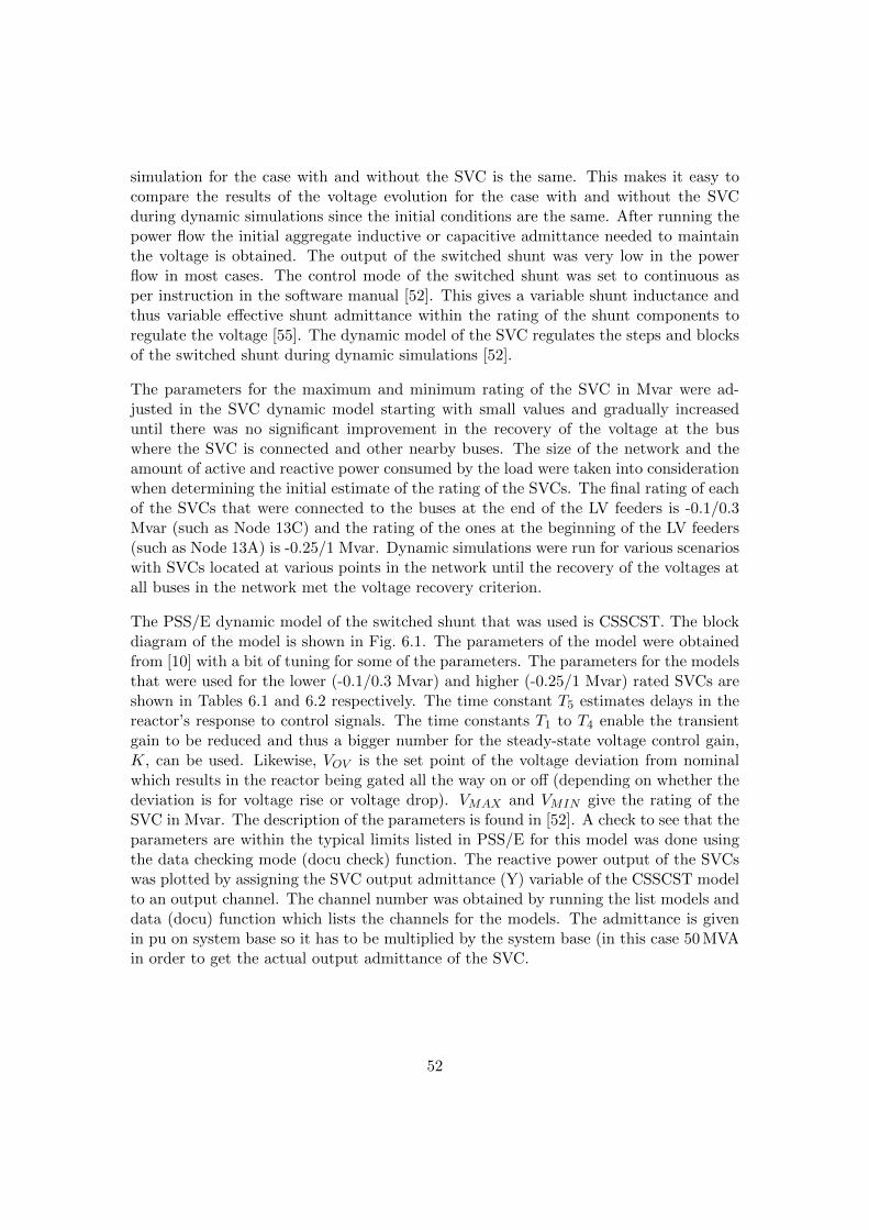
simulation for the case with and without the SVC is the same. This makes it easy tocompare the results of the voltage evolution for the case with and without the SVCduring dynamic simulations since the initial conditions are the same. After running thepower flow the initial aggregate inductive or capacitive admittance needed to maintainthe voltage is obtained. The output of the switched shunt was very low in the powerflow in most cases. The control mode of the switched shunt was set to continuous asper instruction in the software manual [52]. This gives a variable shunt inductance andthus variable effective shunt admittance within the rating of the shunt components toregulate the voltage [55]. The dynamic model of the SVC regulates the steps and blocksof the switched shunt during dynamic simulations [52].

The parameters for the maximum and minimum rating of the SVC in Mvar were ad-justed in the SVC dynamic model starting with small values and gradually increaseduntil there was no significant improvement in the recovery of the voltage at the buswhere the SVC is connected and other nearby buses. The size of the network and theamount of active and reactive power consumed by the load were taken into considerationwhen determining the initial estimate of the rating of the SVCs. The final rating of eachof the SVCs that were connected to the buses at the end of the LV feeders is -0.1/0.3Mvar (such as Node 13C) and the rating of the ones at the beginning of the LV feeders(such as Node 13A) is -0.25/1 Mvar. Dynamic simulations were run for various scenarioswith SVCs located at various points in the network until the recovery of the voltages atall buses in the network met the voltage recovery criterion.

The PSS/E dynamic model of the switched shunt that was used is CSSCST. The blockdiagram of the model is shown in Fig. 6.1. The parameters of the model were obtainedfrom [10] with a bit of tuning for some of the parameters. The parameters for the modelsthat were used for the lower (-0.1/0.3 Mvar) and higher (-0.25/1 Mvar) rated SVCs areshown in Tables 6.1 and 6.2 respectively. The time constant T5 estimates delays in thereactor’s response to control signals. The time constants T1 to T4 enable the transientgain to be reduced and thus a bigger number for the steady-state voltage control gain,K, can be used. Likewise, VOV is the set point of the voltage deviation from nominalwhich results in the reactor being gated all the way on or off (depending on whether thedeviation is for voltage rise or voltage drop). VMAX and VMIN give the rating of theSVC in Mvar. The description of the parameters is found in [52]. A check to see that theparameters are within the typical limits listed in PSS/E for this model was done usingthe data checking mode (docu check) function. The reactive power output of the SVCswas plotted by assigning the SVC output admittance (Y) variable of the CSSCST modelto an output channel. The channel number was obtained by running the list models anddata (docu) function which lists the channels for the models. The admittance is givenin pu on system base so it has to be multiplied by the system base (in this case 50 MVAin order to get the actual output admittance of the SVC.

52

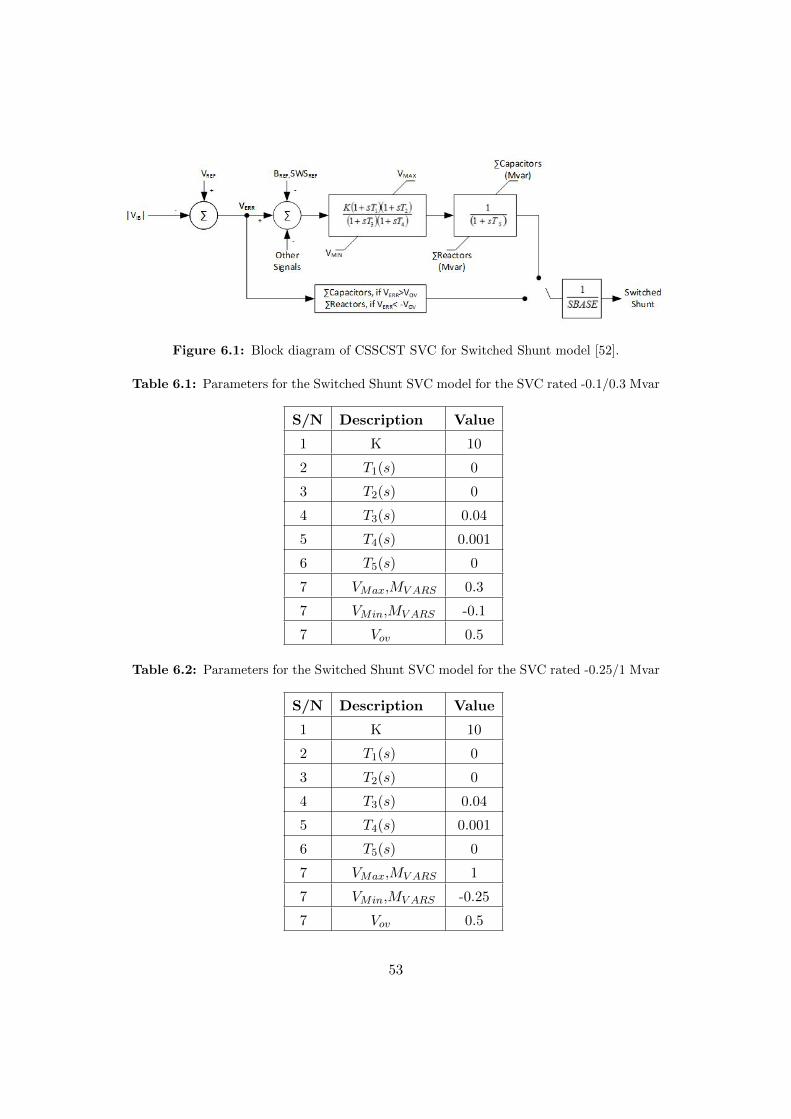
Figure 6.1: Block diagram of CSSCST SVC for Switched Shunt model [52].

Table 6.1: Parameters for the Switched Shunt SVC model for the SVC rated -0.1/0.3 Mvar

S/N Description Value

1 K 10

2 T1(s) 0

3 T2(s) 0

4 T3(s) 0.04

5 T4(s) 0.001

6 T5(s) 0

7 VMax,MV ARS 0.3

7 VMin,MV ARS -0.1

7 Vov 0.5

Table 6.2: Parameters for the Switched Shunt SVC model for the SVC rated -0.25/1 Mvar

S/N Description Value

1 K 10

2 T1(s) 0

3 T2(s) 0

4 T3(s) 0.04

5 T4(s) 0.001

6 T5(s) 0

7 VMax,MV ARS 1

7 VMin,MV ARS -0.25

7 Vov 0.5

53

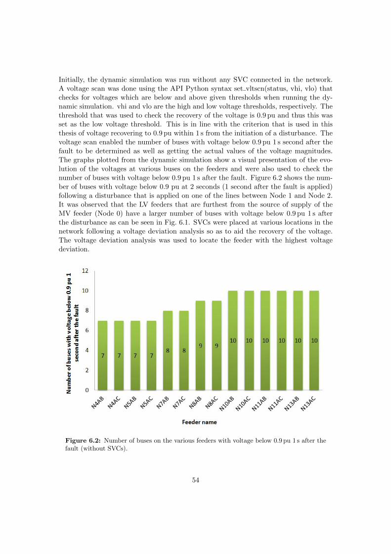
Initially, the dynamic simulation was run without any SVC connected in the network.A voltage scan was done using the API Python syntax set vltscn(status, vhi, vlo) thatchecks for voltages which are below and above given thresholds when running the dy-namic simulation. vhi and vlo are the high and low voltage thresholds, respectively. Thethreshold that was used to check the recovery of the voltage is 0.9 pu and thus this wasset as the low voltage threshold. This is in line with the criterion that is used in thisthesis of voltage recovering to 0.9 pu within 1 s from the initiation of a disturbance. Thevoltage scan enabled the number of buses with voltage below 0.9 pu 1 s second after thefault to be determined as well as getting the actual values of the voltage magnitudes.The graphs plotted from the dynamic simulation show a visual presentation of the evo-lution of the voltages at various buses on the feeders and were also used to check thenumber of buses with voltage below 0.9 pu 1 s after the fault. Figure 6.2 shows the num-ber of buses with voltage below 0.9 pu at 2 seconds (1 second after the fault is applied)following a disturbance that is applied on one of the lines between Node 1 and Node 2.It was observed that the LV feeders that are furthest from the source of supply of theMV feeder (Node 0) have a larger number of buses with voltage below 0.9 pu 1 s afterthe disturbance as can be seen in Fig. 6.1. SVCs were placed at various locations in thenetwork following a voltage deviation analysis so as to aid the recovery of the voltage.The voltage deviation analysis was used to locate the feeder with the highest voltagedeviation.

Figure 6.2: Number of buses on the various feeders with voltage below 0.9 pu 1 s after thefault (without SVCs).

54

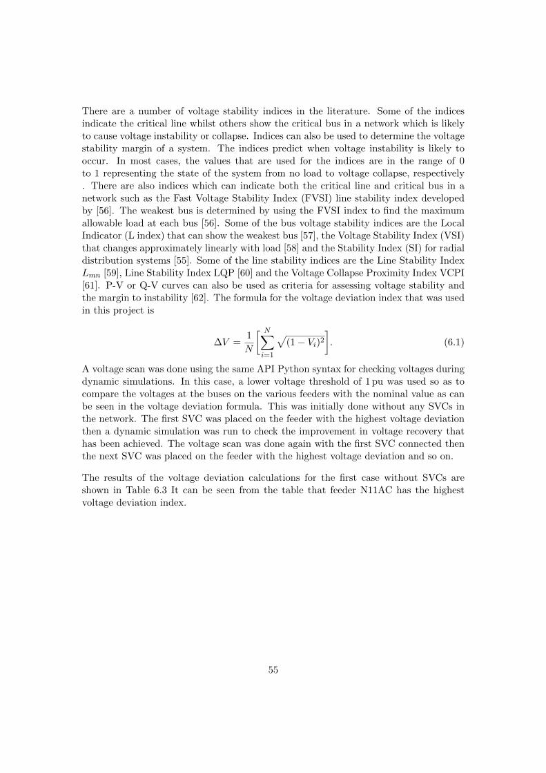
There are a number of voltage stability indices in the literature. Some of the indicesindicate the critical line whilst others show the critical bus in a network which is likelyto cause voltage instability or collapse. Indices can also be used to determine the voltagestability margin of a system. The indices predict when voltage instability is likely tooccur. In most cases, the values that are used for the indices are in the range of 0to 1 representing the state of the system from no load to voltage collapse, respectively. There are also indices which can indicate both the critical line and critical bus in anetwork such as the Fast Voltage Stability Index (FVSI) line stability index developedby [56]. The weakest bus is determined by using the FVSI index to find the maximumallowable load at each bus [56]. Some of the bus voltage stability indices are the LocalIndicator (L index) that can show the weakest bus [57], the Voltage Stability Index (VSI)that changes approximately linearly with load [58] and the Stability Index (SI) for radialdistribution systems [55]. Some of the line stability indices are the Line Stability IndexLmn [59], Line Stability Index LQP [60] and the Voltage Collapse Proximity Index VCPI[61]. P-V or Q-V curves can also be used as criteria for assessing voltage stability andthe margin to instability [62]. The formula for the voltage deviation index that was usedin this project is

∆V =1

N

[ N∑i=1

√(1− Vi)2

]. (6.1)

A voltage scan was done using the same API Python syntax for checking voltages duringdynamic simulations. In this case, a lower voltage threshold of 1 pu was used so as tocompare the voltages at the buses on the various feeders with the nominal value as canbe seen in the voltage deviation formula. This was initially done without any SVCs inthe network. The first SVC was placed on the feeder with the highest voltage deviationthen a dynamic simulation was run to check the improvement in voltage recovery thathas been achieved. The voltage scan was done again with the first SVC connected thenthe next SVC was placed on the feeder with the highest voltage deviation and so on.

The results of the voltage deviation calculations for the first case without SVCs areshown in Table 6.3 It can be seen from the table that feeder N11AC has the highestvoltage deviation index.

55

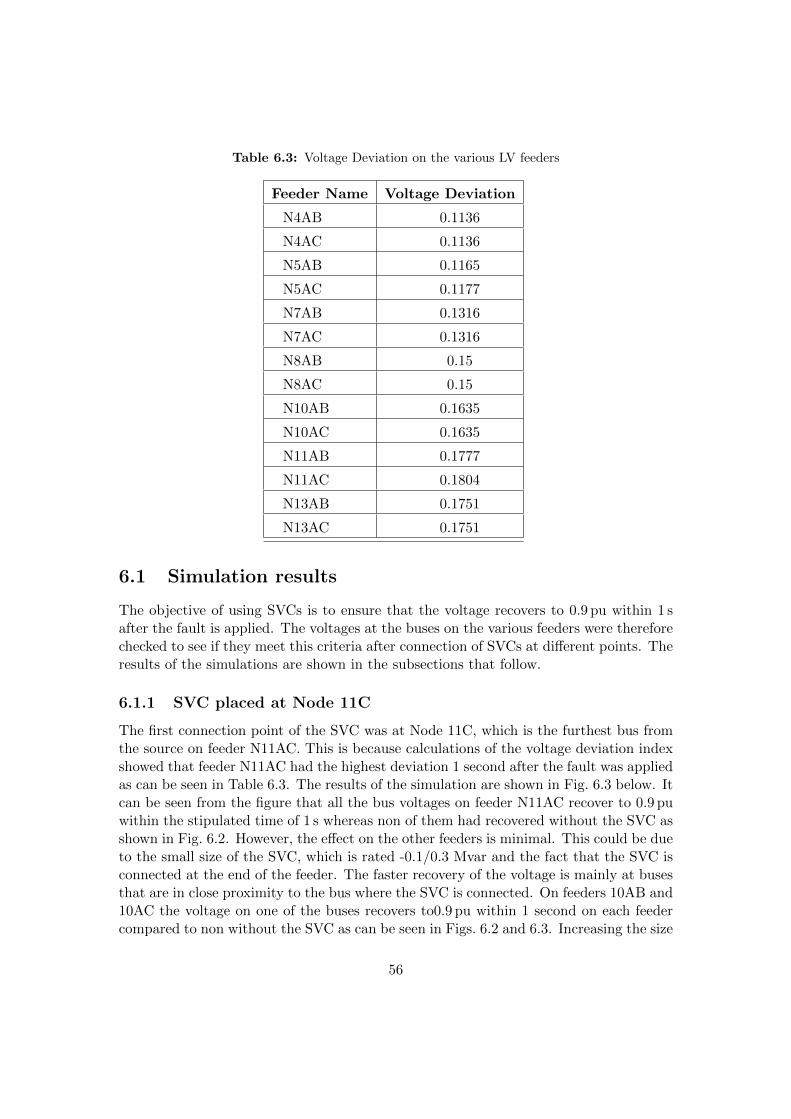
Table 6.3: Voltage Deviation on the various LV feeders

Feeder Name Voltage Deviation

N4AB 0.1136

N4AC 0.1136

N5AB 0.1165

N5AC 0.1177

N7AB 0.1316

N7AC 0.1316

N8AB 0.15

N8AC 0.15

N10AB 0.1635

N10AC 0.1635

N11AB 0.1777

N11AC 0.1804

N13AB 0.1751

N13AC 0.1751

6.1 Simulation results

The objective of using SVCs is to ensure that the voltage recovers to 0.9 pu within 1 safter the fault is applied. The voltages at the buses on the various feeders were thereforechecked to see if they meet this criteria after connection of SVCs at different points. Theresults of the simulations are shown in the subsections that follow.

6.1.1 SVC placed at Node 11C

The first connection point of the SVC was at Node 11C, which is the furthest bus fromthe source on feeder N11AC. This is because calculations of the voltage deviation indexshowed that feeder N11AC had the highest deviation 1 second after the fault was appliedas can be seen in Table 6.3. The results of the simulation are shown in Fig. 6.3 below. Itcan be seen from the figure that all the bus voltages on feeder N11AC recover to 0.9 puwithin the stipulated time of 1 s whereas non of them had recovered without the SVC asshown in Fig. 6.2. However, the effect on the other feeders is minimal. This could be dueto the small size of the SVC, which is rated -0.1/0.3 Mvar and the fact that the SVC isconnected at the end of the feeder. The faster recovery of the voltage is mainly at busesthat are in close proximity to the bus where the SVC is connected. On feeders 10AB and10AC the voltage on one of the buses recovers to0.9 pu within 1 second on each feedercompared to non without the SVC as can be seen in Figs. 6.2 and 6.3. Increasing the size

56

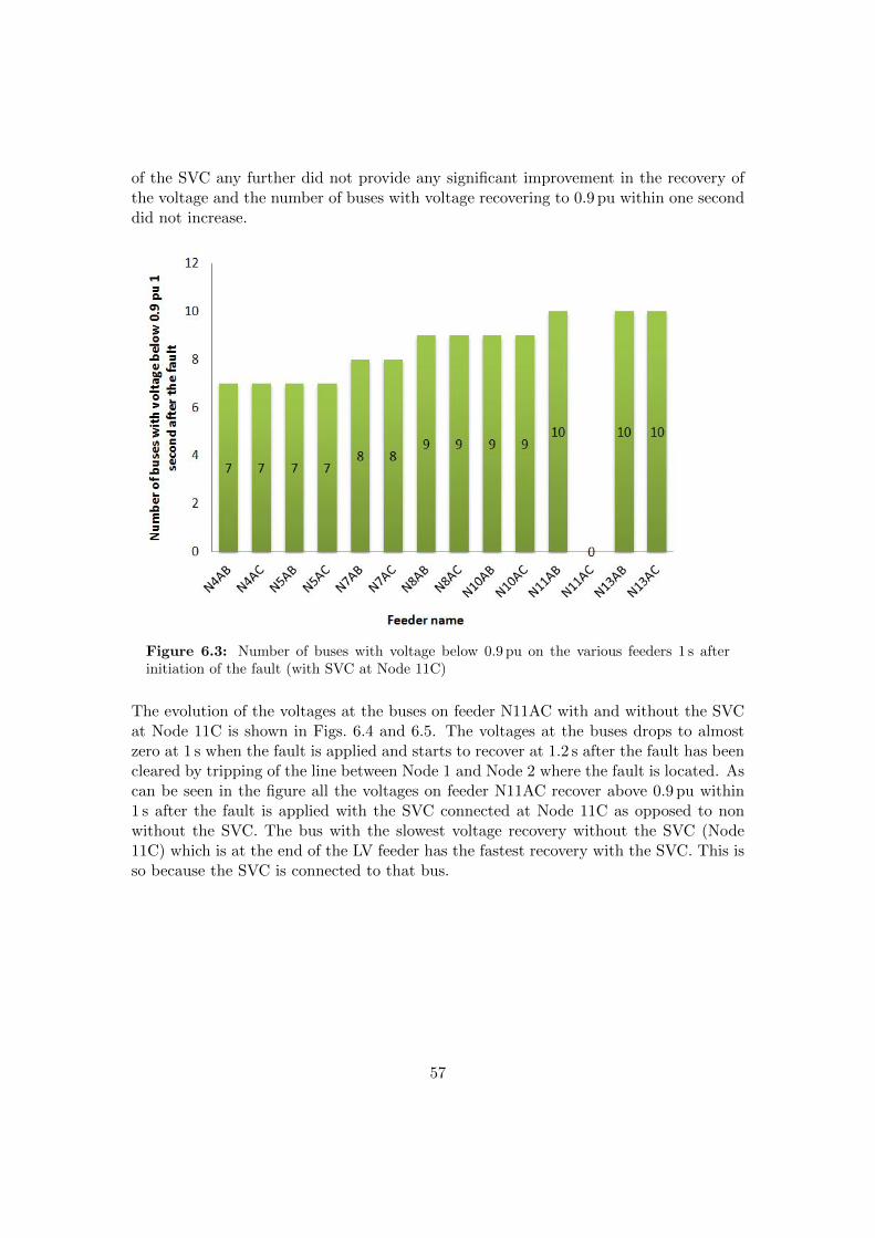
of the SVC any further did not provide any significant improvement in the recovery ofthe voltage and the number of buses with voltage recovering to 0.9 pu within one seconddid not increase.

Figure 6.3: Number of buses with voltage below 0.9 pu on the various feeders 1 s afterinitiation of the fault (with SVC at Node 11C)

The evolution of the voltages at the buses on feeder N11AC with and without the SVCat Node 11C is shown in Figs. 6.4 and 6.5. The voltages at the buses drops to almostzero at 1 s when the fault is applied and starts to recover at 1.2 s after the fault has beencleared by tripping of the line between Node 1 and Node 2 where the fault is located. Ascan be seen in the figure all the voltages on feeder N11AC recover above 0.9 pu within1 s after the fault is applied with the SVC connected at Node 11C as opposed to nonwithout the SVC. The bus with the slowest voltage recovery without the SVC (Node11C) which is at the end of the LV feeder has the fastest recovery with the SVC. This isso because the SVC is connected to that bus.

57

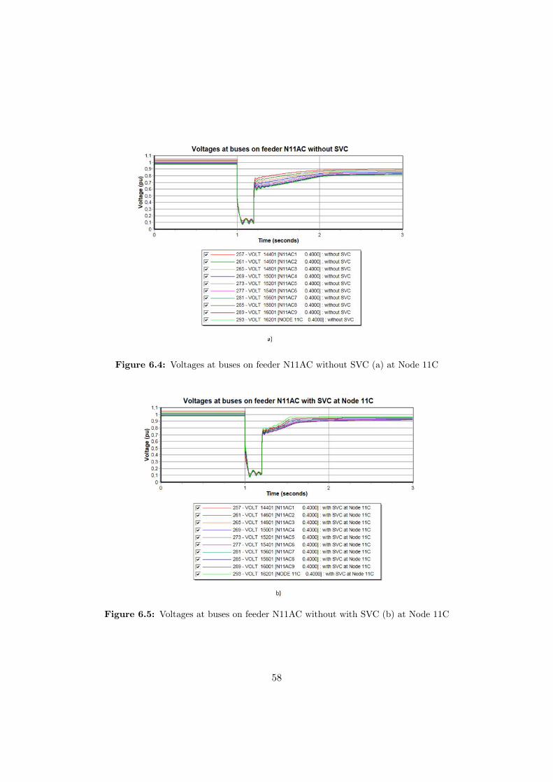
Figure 6.4: Voltages at buses on feeder N11AC without SVC (a) at Node 11C

Figure 6.5: Voltages at buses on feeder N11AC without with SVC (b) at Node 11C

58

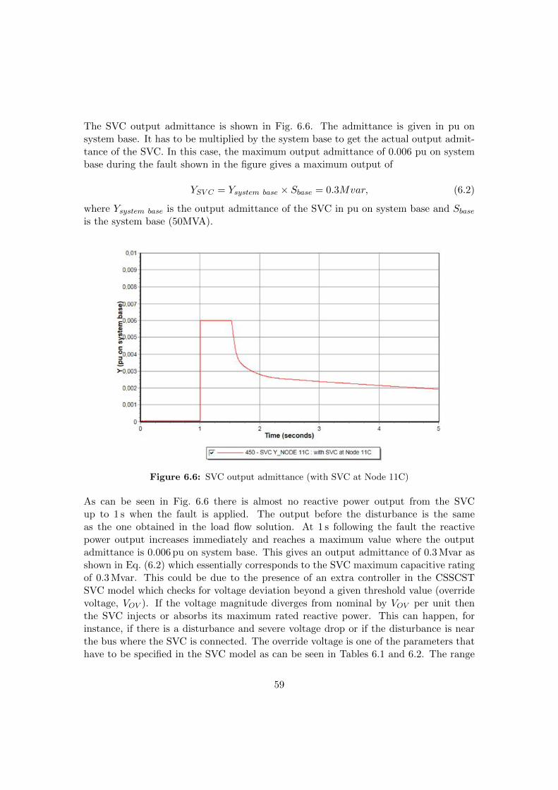
The SVC output admittance is shown in Fig. 6.6. The admittance is given in pu onsystem base. It has to be multiplied by the system base to get the actual output admit-tance of the SVC. In this case, the maximum output admittance of 0.006 pu on systembase during the fault shown in the figure gives a maximum output of

YSV C = Ysystem base × Sbase = 0.3Mvar, (6.2)

where Ysystem base is the output admittance of the SVC in pu on system base and Sbaseis the system base (50MVA).

Figure 6.6: SVC output admittance (with SVC at Node 11C)

As can be seen in Fig. 6.6 there is almost no reactive power output from the SVCup to 1 s when the fault is applied. The output before the disturbance is the sameas the one obtained in the load flow solution. At 1 s following the fault the reactivepower output increases immediately and reaches a maximum value where the outputadmittance is 0.006 pu on system base. This gives an output admittance of 0.3 Mvar asshown in Eq. (6.2) which essentially corresponds to the SVC maximum capacitive ratingof 0.3 Mvar. This could be due to the presence of an extra controller in the CSSCSTSVC model which checks for voltage deviation beyond a given threshold value (overridevoltage, VOV ). If the voltage magnitude diverges from nominal by VOV per unit thenthe SVC injects or absorbs its maximum rated reactive power. This can happen, forinstance, if there is a disturbance and severe voltage drop or if the disturbance is nearthe bus where the SVC is connected. The override voltage is one of the parameters thathave to be specified in the SVC model as can be seen in Tables 6.1 and 6.2. The range

59

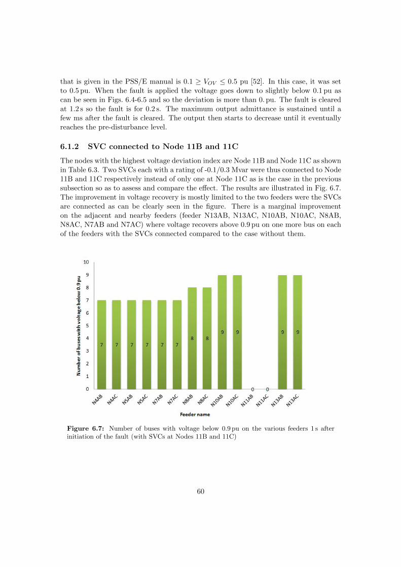
that is given in the PSS/E manual is 0.1 ≥ VOV ≤ 0.5 pu [52]. In this case, it was setto 0.5 pu. When the fault is applied the voltage goes down to slightly below 0.1 pu ascan be seen in Figs. 6.4-6.5 and so the deviation is more than 0. pu. The fault is clearedat 1.2 s so the fault is for 0.2 s. The maximum output admittance is sustained until afew ms after the fault is cleared. The output then starts to decrease until it eventuallyreaches the pre-disturbance level.

6.1.2 SVC connected to Node 11B and 11C

The nodes with the highest voltage deviation index are Node 11B and Node 11C as shownin Table 6.3. Two SVCs each with a rating of -0.1/0.3 Mvar were thus connected to Node11B and 11C respectively instead of only one at Node 11C as is the case in the previoussubsection so as to assess and compare the effect. The results are illustrated in Fig. 6.7.The improvement in voltage recovery is mostly limited to the two feeders were the SVCsare connected as can be clearly seen in the figure. There is a marginal improvementon the adjacent and nearby feeders (feeder N13AB, N13AC, N10AB, N10AC, N8AB,N8AC, N7AB and N7AC) where voltage recovers above 0.9 pu on one more bus on eachof the feeders with the SVCs connected compared to the case without them.

Figure 6.7: Number of buses with voltage below 0.9 pu on the various feeders 1 s afterinitiation of the fault (with SVCs at Nodes 11B and 11C)

60

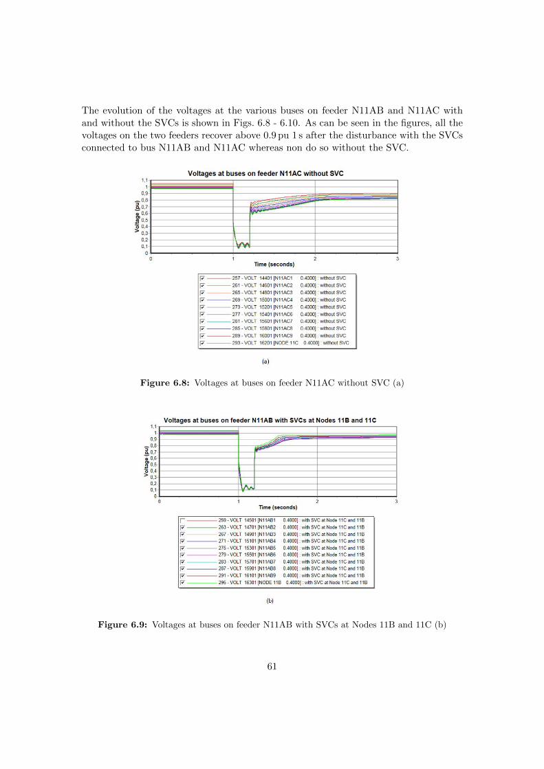
The evolution of the voltages at the various buses on feeder N11AB and N11AC withand without the SVCs is shown in Figs. 6.8 - 6.10. As can be seen in the figures, all thevoltages on the two feeders recover above 0.9 pu 1 s after the disturbance with the SVCsconnected to bus N11AB and N11AC whereas non do so without the SVC.

Figure 6.8: Voltages at buses on feeder N11AC without SVC (a)

Figure 6.9: Voltages at buses on feeder N11AB with SVCs at Nodes 11B and 11C (b)

61

Figure 6.10: Voltages at buses on feeder N11AC with SVCs at Nodes 11B and 11C (c)

From the simulations, the reactive power output for this case for each SVC is similar tothe case shown in Fig. 6.6 where the SVC is connected to Node 11C.

The results presented in the above figures indicated that the improvement in voltagerecovery is mostly limited to the two feeders were the SVCs are connected. Next, thestudy of the Thesis will continue with the connection of the SVC to Node N11AC5.

6.1.3 SVC connected to Node N11AC5

In this case, the SVC was connected to bus N11AC5 which is in the middle of feederN11AC. The results are shown in Fig. 6.11. There is a slightly lower number of buseswith voltage below 0.9 pu 1 second after the fault than the case where the SVC is placedat the end of the feeder. However, the improvement is not significant since the voltageon only one additional bus per feeder recovers above 0.9 pu within 1 second comparedto the case where the SVC is at the end of the feeder. This is apart from feeder N5AC,N10AB and N10AC where the result is the same for the two cases.

62

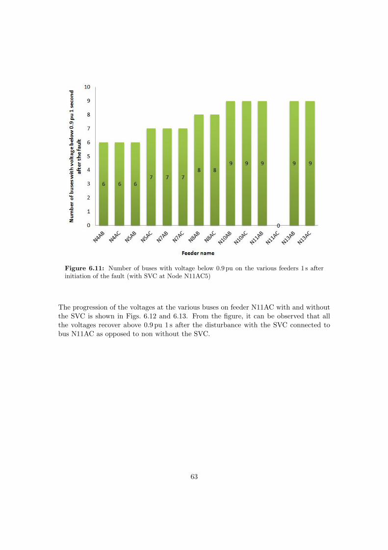
Figure 6.11: Number of buses with voltage below 0.9 pu on the various feeders 1 s afterinitiation of the fault (with SVC at Node N11AC5)

The progression of the voltages at the various buses on feeder N11AC with and withoutthe SVC is shown in Figs. 6.12 and 6.13. From the figure, it can be observed that allthe voltages recover above 0.9 pu 1 s after the disturbance with the SVC connected tobus N11AC as opposed to non without the SVC.

63

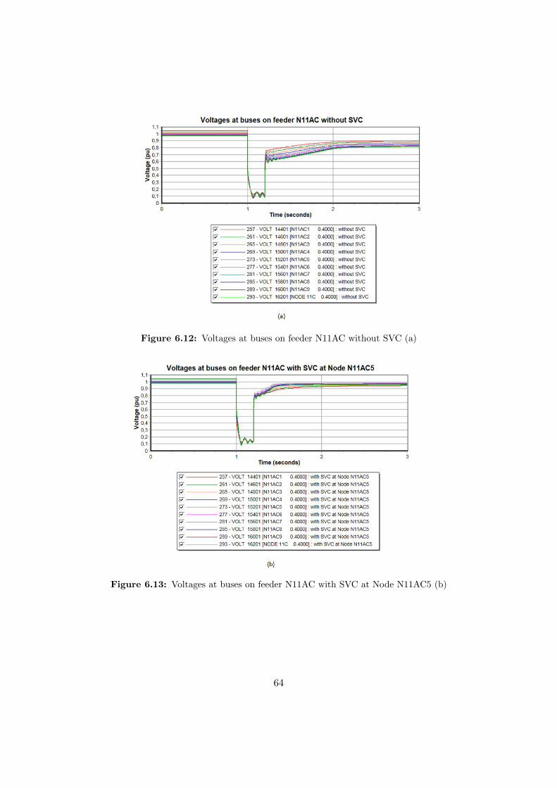
Figure 6.12: Voltages at buses on feeder N11AC without SVC (a)

Figure 6.13: Voltages at buses on feeder N11AC with SVC at Node N11AC5 (b)

64

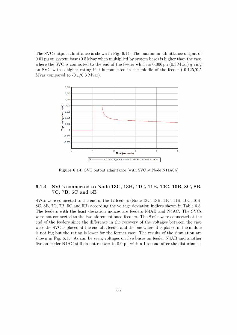
The SVC output admittance is shown in Fig. 6.14. The maximum admittance output of0.01 pu on system base (0.5 Mvar when multiplied by system base) is higher than the casewhere the SVC is connected to the end of the feeder which is 0.006 pu (0.3 Mvar) givingan SVC with a higher rating if it is connected in the middle of the feeder (-0.125/0.5Mvar compared to -0.1/0.3 Mvar).

Figure 6.14: SVC output admittance (with SVC at Node N11AC5)

6.1.4 SVCs connected to Node 13C, 13B, 11C, 11B, 10C, 10B, 8C, 8B,7C, 7B, 5C and 5B

SVCs were connected to the end of the 12 feeders (Node 13C, 13B, 11C, 11B, 10C, 10B,8C, 8B, 7C, 7B, 5C and 5B) according the voltage deviation indices shown in Table 6.3.The feeders with the least deviation indices are feeders N4AB and N4AC. The SVCswere not connected to the two aforementioned feeders. The SVCs were connected at theend of the feeders since the difference in the recovery of the voltages between the casewere the SVC is placed at the end of a feeder and the one where it is placed in the middleis not big but the rating is lower for the former case. The results of the simulation areshown in Fig. 6.15. As can be seen, voltages on five buses on feeder N4AB and anotherfive on feeder N4AC still do not recover to 0.9 pu within 1 second after the disturbance.

65

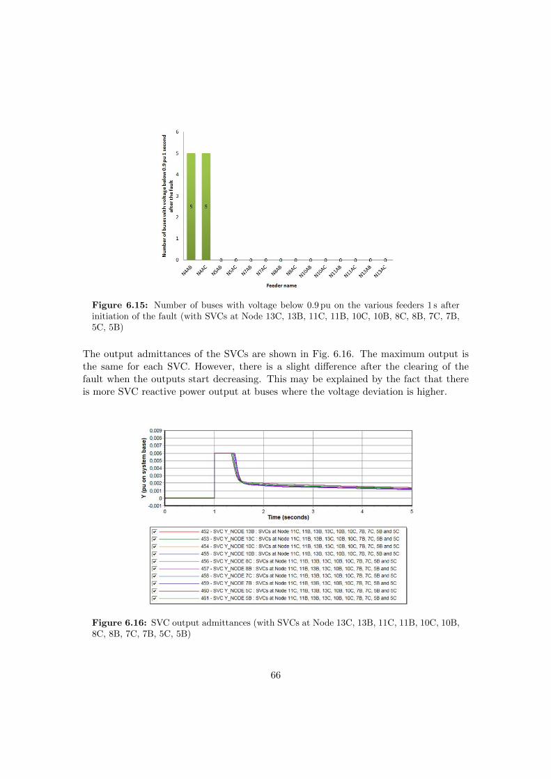
Figure 6.15: Number of buses with voltage below 0.9 pu on the various feeders 1 s afterinitiation of the fault (with SVCs at Node 13C, 13B, 11C, 11B, 10C, 10B, 8C, 8B, 7C, 7B,5C, 5B)

The output admittances of the SVCs are shown in Fig. 6.16. The maximum output isthe same for each SVC. However, there is a slight difference after the clearing of thefault when the outputs start decreasing. This may be explained by the fact that thereis more SVC reactive power output at buses where the voltage deviation is higher.

Figure 6.16: SVC output admittances (with SVCs at Node 13C, 13B, 11C, 11B, 10C, 10B,8C, 8B, 7C, 7B, 5C, 5B)

66

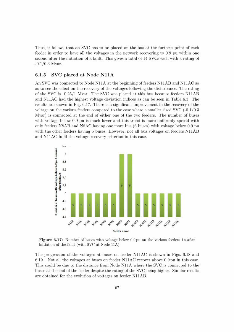
Thus, it follows that an SVC has to be placed on the bus at the furthest point of eachfeeder in order to have all the voltages in the network recovering to 0.9 pu within onesecond after the initiation of a fault. This gives a total of 14 SVCs each with a rating of-0.1/0.3 Mvar.

6.1.5 SVC placed at Node N11A

An SVC was connected to Node N11A at the beginning of feeders N11AB and N11AC soas to see the effect on the recovery of the voltages following the disturbance. The ratingof the SVC is -0.25/1 Mvar. The SVC was placed at this bus because feeders N11ABand N11AC had the highest voltage deviation indices as can be seen in Table 6.3. Theresults are shown in Fig. 6.17. There is a significant improvement in the recovery of thevoltage on the various feeders compared to the case where a smaller sized SVC (-0.1/0.3Mvar) is connected at the end of either one of the two feeders. The number of buseswith voltage below 0.9 pu is much lower and this trend is more uniformly spread withonly feeders N8AB and N8AC having one more bus (6 buses) with voltage below 0.9 puwith the other feeders having 5 buses. However, not all bus voltages on feeders N11ABand N11AC fulfil the voltage recovery criterion in this case.

Figure 6.17: Number of buses with voltage below 0.9 pu on the various feeders 1 s afterinitiation of the fault (with SVC at Node 11A)

The progression of the voltages at buses on feeder N11AC is shown in Figs. 6.18 and6.19 . Not all the voltages at buses on feeder N11AC recover above 0.9 pu in this case.This could be due to the distance from Node N11A where the SVC is connected to thebuses at the end of the feeder despite the rating of the SVC being higher. Similar resultsare obtained for the evolution of voltages on feeder N11AB.

67

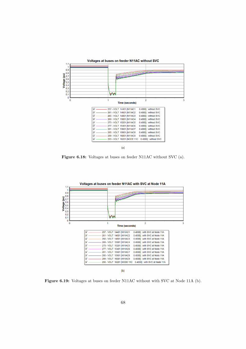
Figure 6.18: Voltages at buses on feeder N11AC without SVC (a).

Figure 6.19: Voltages at buses on feeder N11AC without with SVC at Node 11A (b).

68

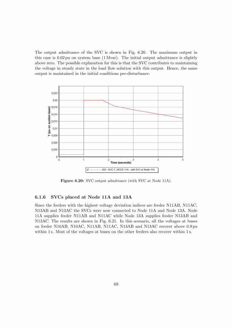
The output admittance of the SVC is shown in Fig. 6.20. The maximum output inthis case is 0.02 pu on system base (1 Mvar). The initial output admittance is slightlyabove zero. The possible explanation for this is that the SVC contributes to maintainingthe voltage in steady state in the load flow solution with this output. Hence, the sameoutput is maintained in the initial conditions pre-disturbance.

Figure 6.20: SVC output admittance (with SVC at Node 11A).

6.1.6 SVCs placed at Node 11A and 13A

Since the feeders with the highest voltage deviation indices are feeder N11AB, N11AC,N13AB and N13AC the SVCs were now connected to Node 11A and Node 13A. Node11A supplies feeder N11AB and N11AC while Node 13A supplies feeder N13AB andN13AC. The results are shown in Fig. 6.21. In this scenario, all the voltages at buseson feeder N10AB, N10AC, N11AB, N11AC, N13AB and N13AC recover above 0.9 puwithin 1 s. Most of the voltages at buses on the other feeders also recover within 1 s.

69

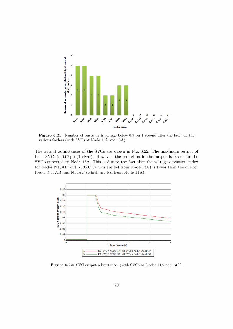
Figure 6.21: Number of buses with voltage below 0.9 pu 1 second after the fault on thevarious feeders (with SVCs at Node 11A and 13A).

The output admittances of the SVCs are shown in Fig. 6.22. The maximum output ofboth SVCs is 0.02 pu (1 Mvar). However, the reduction in the output is faster for theSVC connected to Node 13A. This is due to the fact that the voltage deviation indexfor feeder N13AB and N13AC (which are fed from Node 13A) is lower than the one forfeeder N11AB and N11AC (which are fed from Node 11A).

Figure 6.22: SVC output admittances (with SVCs at Nodes 11A and 13A).

70

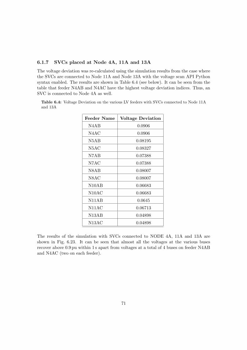
6.1.7 SVCs placed at Node 4A, 11A and 13A

The voltage deviation was re-calculated using the simulation results from the case wherethe SVCs are connected to Node 11A and Node 13A with the voltage scan API Pythonsyntax enabled. The results are shown in Table 6.4 (see below). It can be seen from thetable that feeder N4AB and N4AC have the highest voltage deviation indices. Thus, anSVC is connected to Node 4A as well.

Table 6.4: Voltage Deviation on the various LV feeders with SVCs connected to Node 11Aand 13A

Feeder Name Voltage Deviation

N4AB 0.0906

N4AC 0.0906

N5AB 0.08195

N5AC 0.08327

N7AB 0.07388

N7AC 0.07388

N8AB 0.08007

N8AC 0.08007

N10AB 0.06683

N10AC 0.06683

N11AB 0.0645

N11AC 0.06713

N13AB 0.04898

N13AC 0.04898

The results of the simulation with SVCs connected to NODE 4A, 11A and 13A areshown in Fig. 6.23. It can be seen that almost all the voltages at the various busesrecover above 0.9 pu within 1 s apart from voltages at a total of 4 buses on feeder N4ABand N4AC (two on each feeder).

71

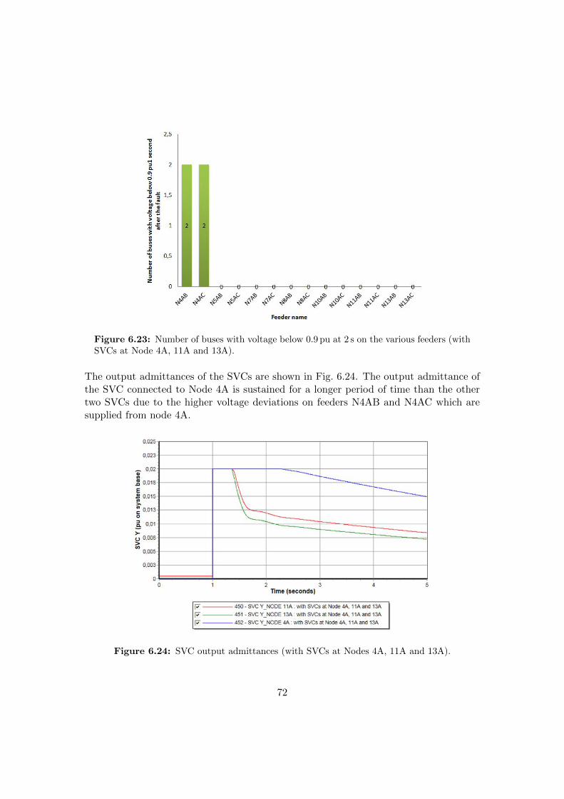
Figure 6.23: Number of buses with voltage below 0.9 pu at 2 s on the various feeders (withSVCs at Node 4A, 11A and 13A).

The output admittances of the SVCs are shown in Fig. 6.24. The output admittance ofthe SVC connected to Node 4A is sustained for a longer period of time than the othertwo SVCs due to the higher voltage deviations on feeders N4AB and N4AC which aresupplied from node 4A.

Figure 6.24: SVC output admittances (with SVCs at Nodes 4A, 11A and 13A).

72

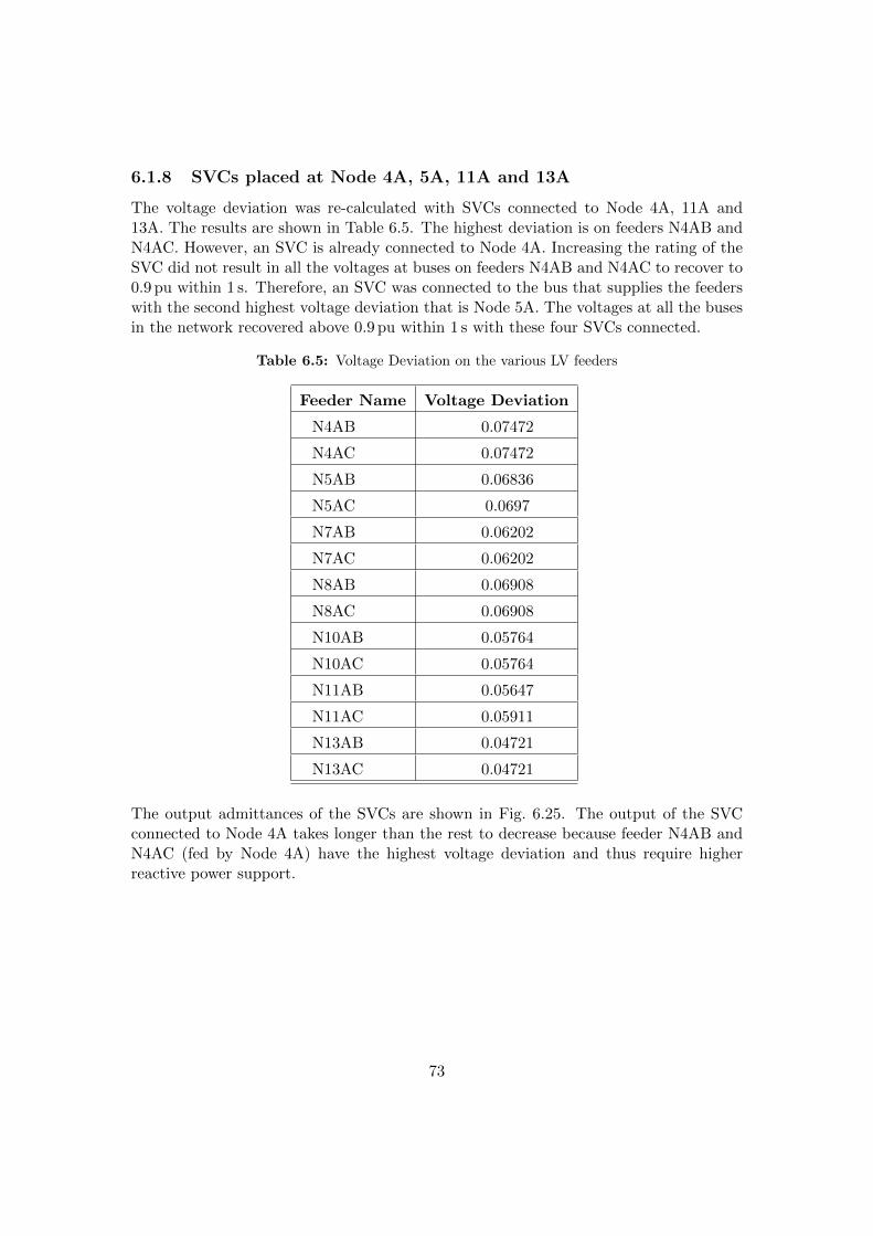
6.1.8 SVCs placed at Node 4A, 5A, 11A and 13A

The voltage deviation was re-calculated with SVCs connected to Node 4A, 11A and13A. The results are shown in Table 6.5. The highest deviation is on feeders N4AB andN4AC. However, an SVC is already connected to Node 4A. Increasing the rating of theSVC did not result in all the voltages at buses on feeders N4AB and N4AC to recover to0.9 pu within 1 s. Therefore, an SVC was connected to the bus that supplies the feederswith the second highest voltage deviation that is Node 5A. The voltages at all the busesin the network recovered above 0.9 pu within 1 s with these four SVCs connected.

Table 6.5: Voltage Deviation on the various LV feeders

Feeder Name Voltage Deviation

N4AB 0.07472

N4AC 0.07472

N5AB 0.06836

N5AC 0.0697

N7AB 0.06202

N7AC 0.06202

N8AB 0.06908

N8AC 0.06908

N10AB 0.05764

N10AC 0.05764

N11AB 0.05647

N11AC 0.05911

N13AB 0.04721

N13AC 0.04721

The output admittances of the SVCs are shown in Fig. 6.25. The output of the SVCconnected to Node 4A takes longer than the rest to decrease because feeder N4AB andN4AC (fed by Node 4A) have the highest voltage deviation and thus require higherreactive power support.

73

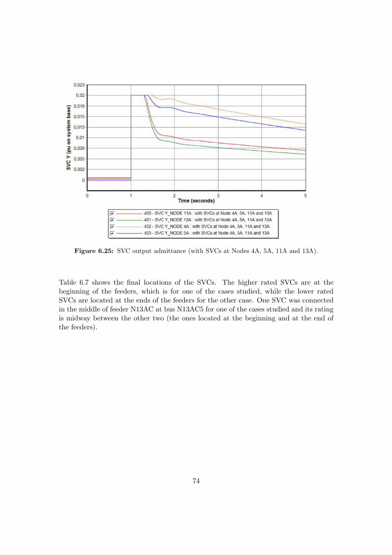
Figure 6.25: SVC output admittance (with SVCs at Nodes 4A, 5A, 11A and 13A).

Table 6.7 shows the final locations of the SVCs. The higher rated SVCs are at thebeginning of the feeders, which is for one of the cases studied, while the lower ratedSVCs are located at the ends of the feeders for the other case. One SVC was connectedin the middle of feeder N13AC at bus N13AC5 for one of the cases studied and its ratingis midway between the other two (the ones located at the beginning and at the end ofthe feeders).

74

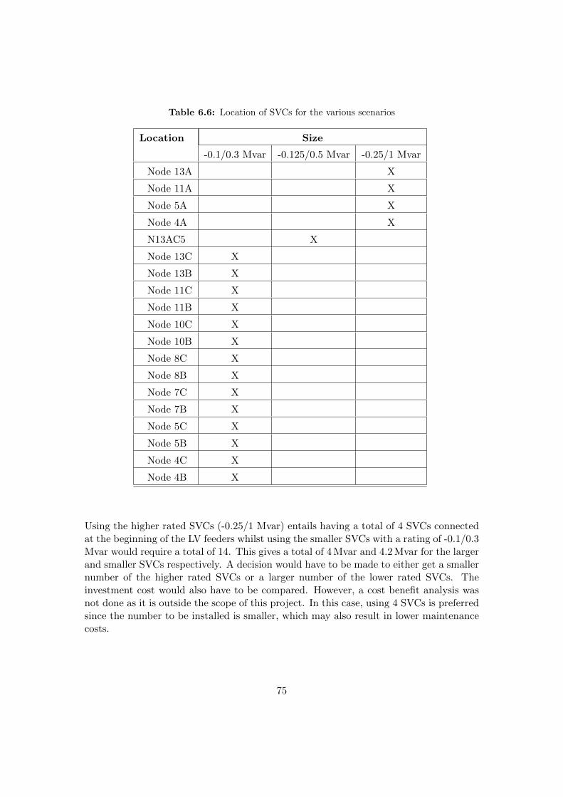
Table 6.6: Location of SVCs for the various scenarios

Location Size

-0.1/0.3 Mvar -0.125/0.5 Mvar -0.25/1 Mvar

Node 13A X

Node 11A X

Node 5A X

Node 4A X

N13AC5 X

Node 13C X

Node 13B X

Node 11C X

Node 11B X

Node 10C X

Node 10B X

Node 8C X

Node 8B X

Node 7C X

Node 7B X

Node 5C X

Node 5B X

Node 4C X

Node 4B X

Using the higher rated SVCs (-0.25/1 Mvar) entails having a total of 4 SVCs connectedat the beginning of the LV feeders whilst using the smaller SVCs with a rating of -0.1/0.3Mvar would require a total of 14. This gives a total of 4 Mvar and 4.2 Mvar for the largerand smaller SVCs respectively. A decision would have to be made to either get a smallernumber of the higher rated SVCs or a larger number of the lower rated SVCs. Theinvestment cost would also have to be compared. However, a cost benefit analysis wasnot done as it is outside the scope of this project. In this case, using 4 SVCs is preferredsince the number to be installed is smaller, which may also result in lower maintenancecosts.

75

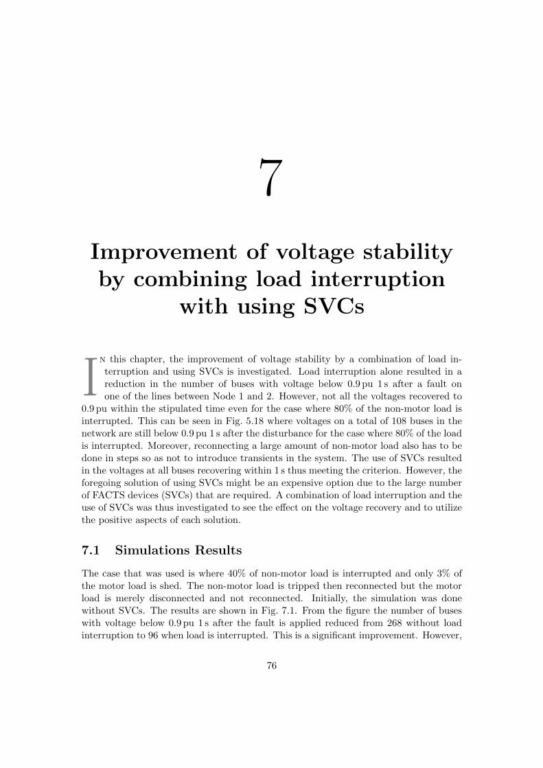
7Improvement of voltage stabilityby combining load interruption

with using SVCs

In this chapter, the improvement of voltage stability by a combination of load in-terruption and using SVCs is investigated. Load interruption alone resulted in areduction in the number of buses with voltage below 0.9 pu 1 s after a fault onone of the lines between Node 1 and 2. However, not all the voltages recovered to

0.9 pu within the stipulated time even for the case where 80% of the non-motor load isinterrupted. This can be seen in Fig. 5.18 where voltages on a total of 108 buses in thenetwork are still below 0.9 pu 1 s after the disturbance for the case where 80% of the loadis interrupted. Moreover, reconnecting a large amount of non-motor load also has to bedone in steps so as not to introduce transients in the system. The use of SVCs resultedin the voltages at all buses recovering within 1 s thus meeting the criterion. However, theforegoing solution of using SVCs might be an expensive option due to the large numberof FACTS devices (SVCs) that are required. A combination of load interruption and theuse of SVCs was thus investigated to see the effect on the voltage recovery and to utilizethe positive aspects of each solution.

7.1 Simulations Results

The case that was used is where 40% of non-motor load is interrupted and only 3% ofthe motor load is shed. The non-motor load is tripped then reconnected but the motorload is merely disconnected and not reconnected. Initially, the simulation was donewithout SVCs. The results are shown in Fig. 7.1. From the figure the number of buseswith voltage below 0.9 pu 1 s after the fault is applied reduced from 268 without loadinterruption to 96 when load is interrupted. This is a significant improvement. However,

76

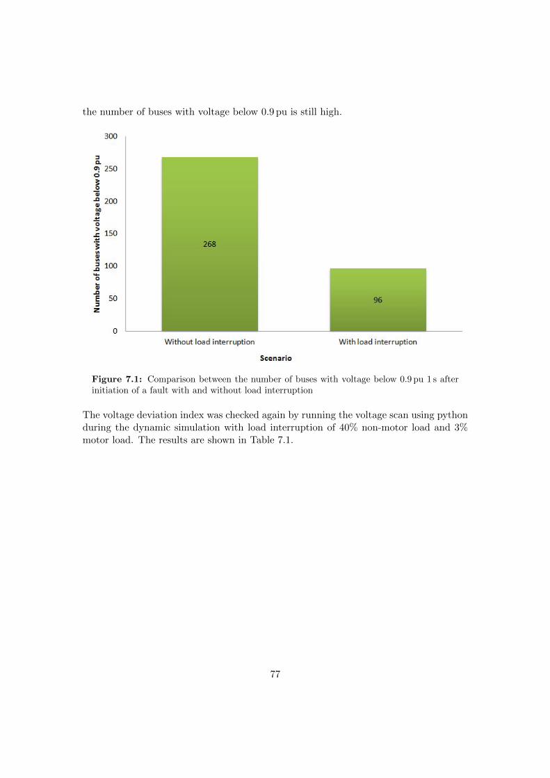
the number of buses with voltage below 0.9 pu is still high.

Figure 7.1: Comparison between the number of buses with voltage below 0.9 pu 1 s afterinitiation of a fault with and without load interruption

The voltage deviation index was checked again by running the voltage scan using pythonduring the dynamic simulation with load interruption of 40% non-motor load and 3%motor load. The results are shown in Table 7.1.

77

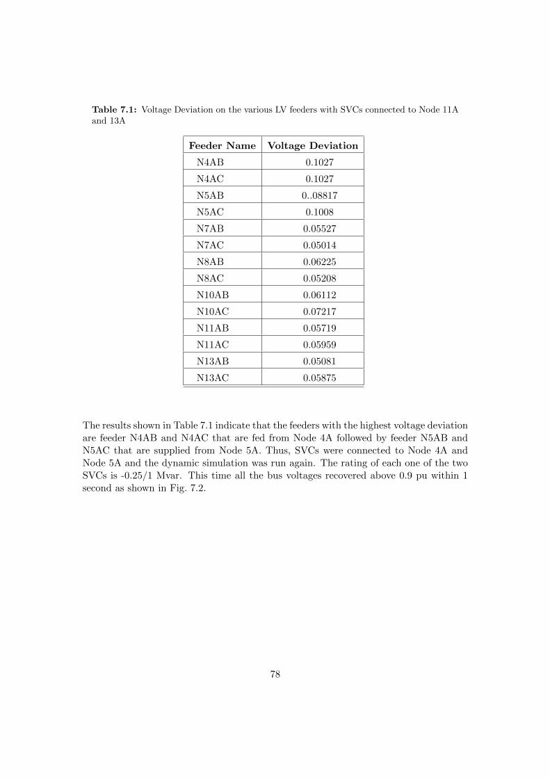
Table 7.1: Voltage Deviation on the various LV feeders with SVCs connected to Node 11Aand 13A

Feeder Name Voltage Deviation

N4AB 0.1027

N4AC 0.1027

N5AB 0..08817

N5AC 0.1008

N7AB 0.05527

N7AC 0.05014

N8AB 0.06225

N8AC 0.05208

N10AB 0.06112

N10AC 0.07217

N11AB 0.05719

N11AC 0.05959

N13AB 0.05081

N13AC 0.05875

The results shown in Table 7.1 indicate that the feeders with the highest voltage deviationare feeder N4AB and N4AC that are fed from Node 4A followed by feeder N5AB andN5AC that are supplied from Node 5A. Thus, SVCs were connected to Node 4A andNode 5A and the dynamic simulation was run again. The rating of each one of the twoSVCs is -0.25/1 Mvar. This time all the bus voltages recovered above 0.9 pu within 1second as shown in Fig. 7.2.

78

Figure 7.2: Number of buses with voltage below 0.9 pu 1 s after initiation of a fault withoutload interruption, with load interruption and a combination of load interruption and using2 SVCs.

From the results, it can be deduced that combining load interruption with the use ofSVCs results in a reduction of the amount of load that has to be interrupted. In thiscase, load interruption of more than 40% of the non-motor load and load shedding ofmore than 3% of the motor load can be avoided. Load interruption can also be donein combination with the use of SVCs without any load shedding at all. Moreover, thenumber of SVCs required to ensure that all the bus voltages recover within 1 s has beenreduced from 4 to 2. This entails a significant saving on the investment capital requiredsince the number of FACTS devices reduces by half. The basic idea that has beenobserved is that the more the load that is interrupted the less the number of SVCs thatare required and vice versa. The proportion of load to be interrupted and the number ofSVCs to install can be decided depending on the prevailing situation and the preferredoptions.

79

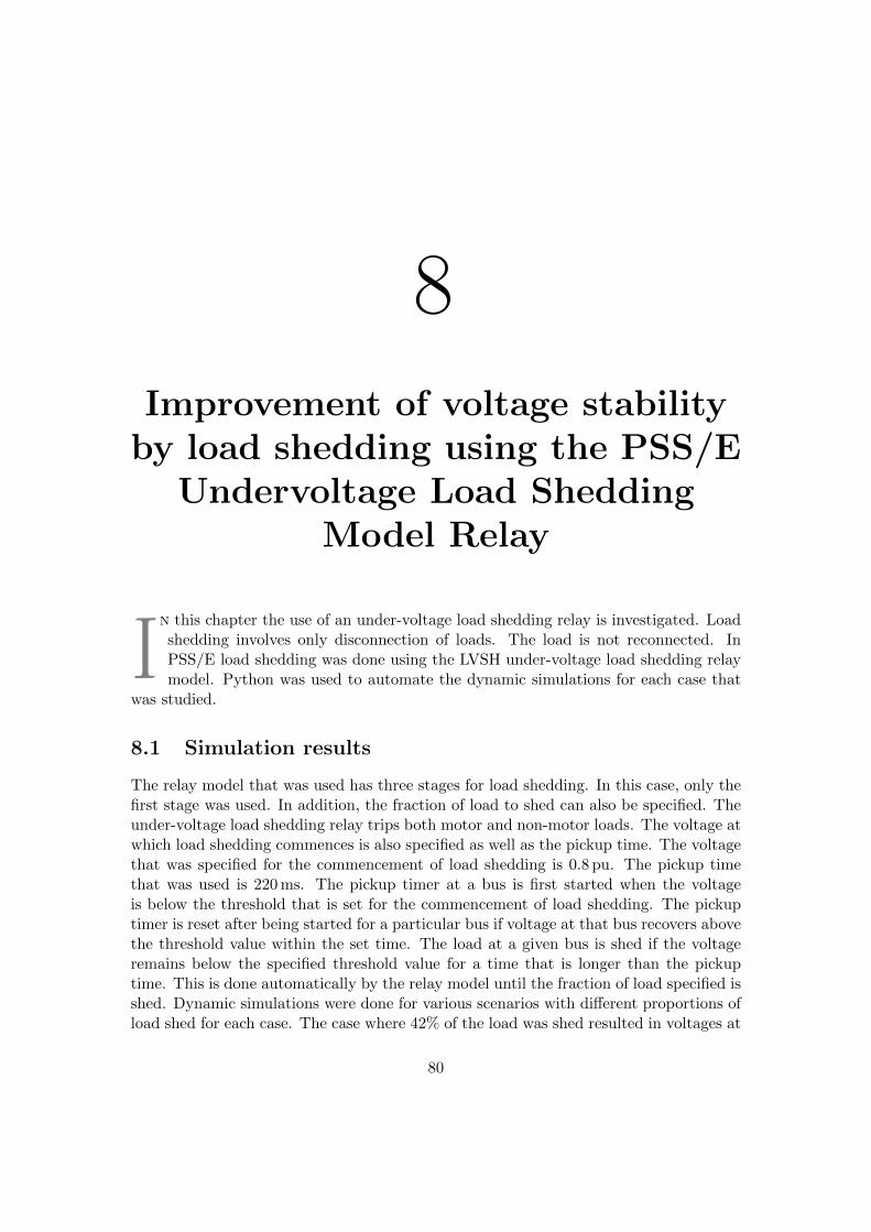
8Improvement of voltage stability

by load shedding using the PSS/EUndervoltage Load Shedding

Model Relay

In this chapter the use of an under-voltage load shedding relay is investigated. Loadshedding involves only disconnection of loads. The load is not reconnected. InPSS/E load shedding was done using the LVSH under-voltage load shedding relaymodel. Python was used to automate the dynamic simulations for each case that

was studied.

8.1 Simulation results

The relay model that was used has three stages for load shedding. In this case, only thefirst stage was used. In addition, the fraction of load to shed can also be specified. Theunder-voltage load shedding relay trips both motor and non-motor loads. The voltage atwhich load shedding commences is also specified as well as the pickup time. The voltagethat was specified for the commencement of load shedding is 0.8 pu. The pickup timethat was used is 220 ms. The pickup timer at a bus is first started when the voltageis below the threshold that is set for the commencement of load shedding. The pickuptimer is reset after being started for a particular bus if voltage at that bus recovers abovethe threshold value within the set time. The load at a given bus is shed if the voltageremains below the specified threshold value for a time that is longer than the pickuptime. This is done automatically by the relay model until the fraction of load specified isshed. Dynamic simulations were done for various scenarios with different proportions ofload shed for each case. The case where 42% of the load was shed resulted in voltages at

80

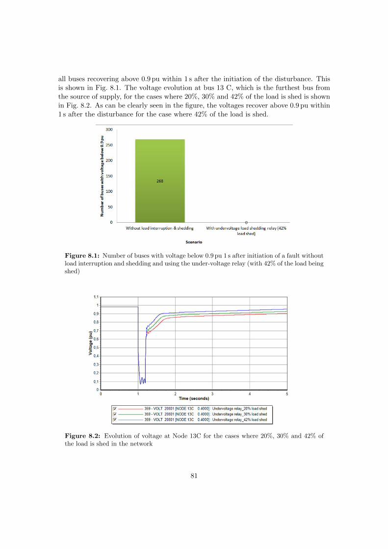
all buses recovering above 0.9 pu within 1 s after the initiation of the disturbance. Thisis shown in Fig. 8.1. The voltage evolution at bus 13 C, which is the furthest bus fromthe source of supply, for the cases where 20%, 30% and 42% of the load is shed is shownin Fig. 8.2. As can be clearly seen in the figure, the voltages recover above 0.9 pu within1 s after the disturbance for the case where 42% of the load is shed.

Figure 8.1: Number of buses with voltage below 0.9 pu 1 s after initiation of a fault withoutload interruption and shedding and using the under-voltage relay (with 42% of the load beingshed)

Figure 8.2: Evolution of voltage at Node 13C for the cases where 20%, 30% and 42% ofthe load is shed in the network

81

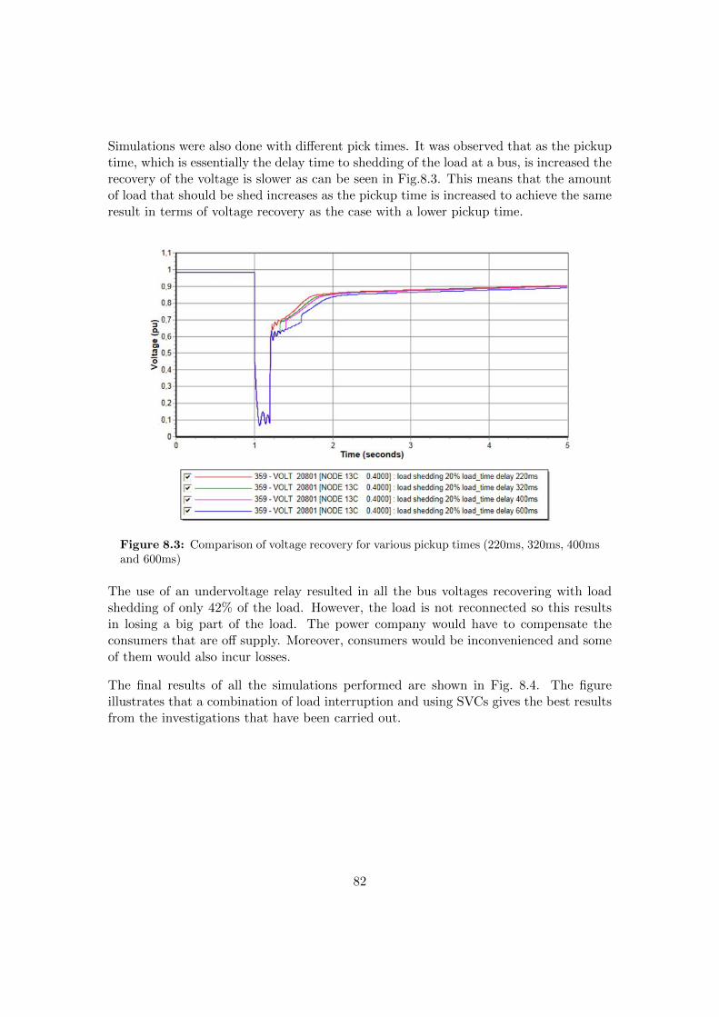
Simulations were also done with different pick times. It was observed that as the pickuptime, which is essentially the delay time to shedding of the load at a bus, is increased therecovery of the voltage is slower as can be seen in Fig.8.3. This means that the amountof load that should be shed increases as the pickup time is increased to achieve the sameresult in terms of voltage recovery as the case with a lower pickup time.

Figure 8.3: Comparison of voltage recovery for various pickup times (220ms, 320ms, 400msand 600ms)

The use of an undervoltage relay resulted in all the bus voltages recovering with loadshedding of only 42% of the load. However, the load is not reconnected so this resultsin losing a big part of the load. The power company would have to compensate theconsumers that are off supply. Moreover, consumers would be inconvenienced and someof them would also incur losses.

The final results of all the simulations performed are shown in Fig. 8.4. The figureillustrates that a combination of load interruption and using SVCs gives the best resultsfrom the investigations that have been carried out.

82

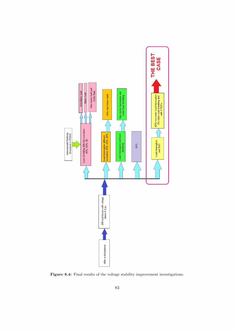
Figure 8.4: Final results of the voltage stability improvement investigations.

83

9Conclusions and Future Work

9.1 Conclusions

The presence of low inertia induction motors in a distribution network may leadto voltage instability after a severe disturbance. Therefore, measures have tobe implemented to reduce the possibility of voltage collapse and to meet thegrid requirements. Studies have to be undertaken to assess the vulnerability

of a system to voltage instability. Different methods can be implemented to help thevoltage to recover faster following a disturbance. Some of the methods that can be usedare load shedding, load interruption, undervoltage relay load shedding and using FACTSdevices such as SVCs. A combination of some of these methods can lead to better re-sults.During this thesis different methods were investigated and implemented on a test net-work to see their effects regarding the improvement of voltage stability. The results showthat the number of load buses with voltages that recovered to 0.9 pu in 1 second arealmost the same for load shedding and load interruption of non-motors loads. However,the load is disconnected for load shedding unlike the case for interruption where all theloads are reconnected back to the system after a few seconds. For instance, the amountof load saved for the case where 60% of the non-motor load is interrupted is 84. Loadinterruption is therefore a good solution but the fraction of load interrupted can be high.It was observed that reconnection of motors is not practical because it introduces a se-vere disturbance in the system. This could be because of the small inertia constant ofthe motors which makes them liable to stall within a short time thereby drawing a lotof current and depressing the voltage further if reconnection is attempted.It was seen that combining load interruption of non-motor loads with load shedding ofmotors resulted in voltage at more load buses recovering to 0.9 pu within 1 sec. Loadshedding therefore aids the voltage recovery but it may be expensive and inconvenientbecause the loads are not reconnected back. It was observed that SVCs offer fast support

84

for voltage recovery and all voltages recover above 0.9 pu within 1 second but severaldevices are required. This might entail huge capital injection. By combining load inter-ruption with the use of SVCs the amount of load interrupted is reduced and the numberof SVCs required is also reduced. This leads to a better overall scheme. Therefore, acombination of load interruption and using SVCs is the best solution. The two methodscomplement each other. Fewer loads are interrupted and the number of SVCs installedto improve the recovery of the voltage can be reduced thereby lowering the investmentcost.

9.2 Future Work

The following future works are proposed for this project:

• A cost benefit analysis of either using SVCs or load interruption so as to comparethe costs of the two methods.

• Further automation of the algorithm for load interruption in Python.

• Performing the simulations using a different software such as DIgSILENT Power-factory so as to compare the results.

• Investigating the use of different types of FACTS devices such as STATCOM foraiding the voltage recovery.

• Performing simulations on a large transmission system supplying distribution net-works with large amounts of motor loads.

85

References

[1] Siemens Industry Inc. Program Operation Manual. Siemens Power TechnologiesInternational, October 2013.

[2] T. Van Cutsem, C. Moors, and D. Lefebvre. Design of load shedding schemesagainst voltage instability using combinatorial optimization. Power EngineeringSociety Winter Meeting, IEEE, 2:848–853, 2002.

[3] Lecture no. 9 in Power System Operation. Voltage Stability (part 1). ChalmersUniversity of Technology, Gothenburg, 2013.

[4] NERC Transmission Issues Subcommittee Subcommittee, System Protection, andControl. A technical reference paper fault - induced delayed voltage recovery, May2014.

[5] B. Otomega and T. Van Cutsem. Distributed load interruption and shedding againstvoltage delayed recovery or instability. PowerTech (POWERTECH), IEEE, pages1–6, 2013.

[6] B. Otomega and T. Van Cutsem. Undervoltage load shedding using distributedcontrollers. IEEE Transactions on Power Systems, 22(4):1898 –1907, 2007.

[7] C.W. Taylor. Power system voltage stability. McGraw-Hill Ryerson, Limited, 1994.

[8] T. Van Cutsem and C. Vournas. Voltage Stability of Electric Power Systems.Springer Science & Business Media, 1998.

[9] C.W. Taylor. Concepts of undervoltage load shedding for voltage stability. PowerEngineering Society Winter Meeting, IEEE, 7:480–488, 1992.

[10] Jamal A. Yasin Ismail A. Hamzah. Static var compensators (svc) required to solvethe problem of delayed voltage recovery following faults in the power system of thesaudi electricity company, western region (sec-wr). Volume:4, 2003.

86

[11] IEEE/CIGRE joint task force on stability terms and definitions. Definition andclassification of power system stability. IEEE Transacctions on Power Systems,19(3):1387–1401, 2004.

[12] T. Van Cutsem. Voltage instability: phenomena, countermeasures, and analysismethods. IEEE Proceedings, 88(2):208–227, 2000.

[13] and E.H. Camm. V. Stewart. Modeling of stalled motor loads for power systemshort-term voltage stability analysis. , IEEE Power Engineering Society GeneralMeeting, 2:1887–1892, 2005.

[14] E.G. Potamianakis and C.D. Vournas. Short-term voltage instability: effects onsynchronous and induction machines. IEEE Transacctions on Power Systems,21(2):791–798, 2006.

[15] NARAIN G., HINGORANI, and LASZLO GYUGYI. Understanding FACTS: con-cepts and technology of Flexible AC Transmission Systems. Wiley-IEEE Press, 2000.

[16] RAJ, P.V., and M. SUDHAKARAN. Optimum load shedding in power systemsstrategies with voltage stability indicators. Engineering, 2:12–21, 2010.

[17] MARAM and . ET. Al. M, D. An optimal load cut policy with event-driven designagainst voltage stability using theta-particle swarm optimization. Journal of Basicand Applied Scientific Research, 3(3):91–100, 2013.

[18] L. ZHIPENG, FUSHUAN, and LEDWICH G. W. An optimal under-frequency loadshedding strategy considering distributed generators and load static characteristics.International Transactions on Electrical Energy Systems, 24(1):75–90, 2014.

[19] P. WANG and BILLINTON R. Optimum load-shedding technique to reduce thetotal customer interruption cost in a distribution system. IEE Proc-Genrr. Transm.Distrib., 147(1):51–57, 2002.

[20] L.P. HAJDU, J. PESCHON, W.F. TINNEY, and D.S.: PIERCY. Optimum load-shedding policy for power systems. International Transactions on Electrical EnergySystems , IEEE Trans, 87(3):784–795, 1968.

[21] ET.AL MOSTAFA, M.A. Optimal dynamic load shedding using a newton baseddynamic algorithm. Electric Power System Research, 34(3):157–163, 1995.

[22] D.K. SUBRAMANIAN. Optimum load shedding through programming techniques.IEEE Trms, 90(I):89–94, 1971.

[23] CHAN and YIP E. S.M. A solution of the transmission limited dispatch problemby sparse linear programming. , IEEE Trans, 98:1044–1053, 1979.

[24] D. DEVARAJ and J.P. ROSELYN. Genetic algorithm based reactive power dispatchfor voltage stability improvement. International Journal of Electrical Power andEnergy Systems., 32(10):1151–1156, 2010.

87

[25] EL ARINI MAHDI. Optimal dynamic load shedding policy for generation loadimbalances including characteristics of loads. International Journal of Energy Re-search, 23(1):79–89, 1999.

[26] MOMOH, ZHU. J.Z. J.A., and S.S. KADDAH. Optimal load shedding study ofnaval-ship power system using the everett optimization technique’. Electric PowerSystems Research, 60(3):145–152, 2002.

[27] VRAKOUPOULU and ANDERSSON G. M. An adaptive load shedding techniquefor controlled islanding. To be publish.

[28] DING XU and GIRGIS A.A. Optimal load shedding strategy in power systems withdistributed geneation. IEEE Power Engineering Society Winter Meeting, 2:788–793,2001.

[29] KARIMI and ET. AL. M. Combination of adaptive and intelligent load sheddingtechniques for distribution network. Power Engineering and Optimization Confer-ence (PEDCO) Melaka, Malaysia, 2012 Ieee International, pages 57–61, 2012.

[30] A.G. BEVRANI, TIKDARI, and HIYAMA. A.G. Power system load shedding: Keyissues and new perspectives. World Academy Science, Engineering and Technology,4:161–166, 2010.

[31] J. LIU, C.H. XIA, SHROFF, and H.D. N.B., SHERALI. Distributed Optimal LoadShedding for Disaster Recovery in Smart Electric Power Grids: A second-OrderApproach.

[32] O. ] ZIAEE and ET. AL. An optimal pricing policy for interruptible load contractsin power markets: A case study for iran. Energy and Power, 1(1):14–20, 2011.

[33] Peter Crossley, Franc Ilar, and Daniel Karlsson. System protection schemes in powernetworks, 2001.

[34] Bogdan Cutsem, Thiery Van; Otomega. Distributed load interruption and sheddingagainst voltage delayed recovery or instability. 2013.

[35] V. Sermanson T. Van Cutsem B. Otomega F. Capitanescu, H. Lefebvre. Prospects ofan improved system protection scheme against voltage instability in the rte system.2008.

[36] Bogdan Otomega Thiery Van Cutsem. Local vs. wide-area undervoltage load shed-ding in the presence of induction motor loads, 2009.

[37] Bogdan Otomega Thiery Van Cutsem. A load shedding scheme against both short-and long-term volatge instabilities in the presence of induction motors. 2011.

[38] Robert A. Jones Lee Y. Taylor S. Mark Halpin, Keith Harley. Slope-permissiveunder-voltage load shed relay for delayed voltage recovery mitigation. 2008.

88

[39] Venkataramana Ajjarapu Hua Bai. A novel online load shedding strategy fo miti-gating fault-induced delayed voltage recovery. Volume:26 , Issue: 1, 2004.

[40] R; Birsa J; RIggle M.; Takeda M; Teramoto H.; Kono Y.; Temma K; Yasuda S;Wofford K; Attaway P.; Lawson J. Sullivan, D; Pape. Managing fault-induceddelayed voltage recorvery in metro atlanta with the burrow county svc. 2009.

[41] D Vassilis, C.; Costas Vournas. Design strategies for load-shedding schemes againstvoltage collapse in the hellenic system. Volume:23 , Issue: 2, 2008.

[42] P. Chen and B. Bak-Jensen. Z. Chen. Comparison of steady-state svc models inload flow calculations. IEEE Universities Power Engineering Conference, pages 1–5,2008.

[43] FACTS terms, DC definitions task force, FACTS working group, and FACTS sub-committee. Proposed terms and definitions for flexible ac transmission system(facts). IEEE Transactions on Power Delivery, 12(4):1848–1853, 1997.

[44] H. Ambriz-Perez, E. Acha, and C.R. Fuerte-Esquivel. Advanced svc models fornewton-raphson load flow and newton optimal power flow studies’. IEEE Transac-tions on Power Systems, 15(I):129–136, 2000.

[45] R.J. Koessler. Dynamic simulation of static var compensators in distribution net-works. IEEE Transacctions on Power Systems, 7(3):1285–1291, 1994.

[46] J.L. MCAVOY. W.K. WONG, D.L. OSBORN. Application of compact static varcompensator solves voltage-flactuation problem. IEEE Transactions on Power De-livery, 5(2):1113–1120, 1990.

[47] Task Force No. 2 on SVC. CIGRE Working Group 38-01. Static var compensator.IEEE Transacctions on Power Systems, 9(1):229–240, 1994.

[48] Task Force No. 2 on SVC. CIGRE Working Group 38-01. Static Var Compensators.I.A. Erinmez, 1986.

[49] Stephen J Chapman. Electric Machinery Fundamentals.

[50] Induction motor.

[51] A Hughes published. Electric Motors and Drives.

[52] Siemens Power Technologies International. Program application guide Volume 2.

[53] Siemens Power Technologies International. MODEL LIBRARY.

[54] Wikipedia, “python (programming language).

[55] Siemens Power Technologies International. Program Application Guide Volume 1.

89

[56] L. MUSIRIN and T.K.A RAHMAN. On-line voltage stability based contingencyranking using fast voltage stability index (fvsi). Transmission and DistributionConference and Exhibition, 2002, 2:1118–1123, 2002.

[57] P. KESSEL and H. GLAVITSCH. Estimating the voltage stability of a powersystem. IEEE Transactions on Power Delivery, 1(3):346–354, 1986.

[58] M.H. HAQUE. Use of local information to determine the distance to voltage col-lapse. Power Engineering Conference, pages 408–413, 2007.

[59] M. MOGHAVVEMI. Technique for contingency monitoring and voltage col-lapse prediction. Generation, Transmission and Distribution IEE Proceedings,145(6):634–640, 1998.

[60] A. MOHAMED, G.B. JASMON, and S. YUSOFF. A static voltage collapse in-dicator using line stability factors. Journal of Industrial Technology, 7(1):73–85,1989.

[61] M. Moghavvemi and O. Faruque. Real–time contingency evaluation and rankingtechnique. Generation, Transmission and Distribution IEE Proceedings, 145(5):517–524, 1998.

[62] C. REIS and F.C. MACIEL BARBOSA. A comparison of voltage stability indices’.Electrotechnical Conference, 21:1007–1010, 2006.

90

ADistribution Network

Figure A.1

91

BPython Scripts

Python script for dynamic simulations without load interruption or SVCs

import os,sys PYTHONPATH = r’C:\Program Files (x86)\PTI\PSSE33 \PSSBIN’MODELFOLDER = r’C:\Program Files (x86)\PTI\PSSE33\MODELDRW’sys.path.append(PYTHONPATH)os.environ[’PATH’] += ’;’ + PYTHONPATHimport psspyimport redirect#import pssepath#pssepath.add pssepath()#import psspy# Redirect output from PSSE to Python:redirect.psse2py()# Last case:CASE = r”D:\Base case without load interruption or SVCs\50% load.sav”psspy.psseinit(12000)psspy.case(CASE)# Convert loads (3 step process):psspy.conl(-1,1,1)psspy.conl(-1,1,2,[0,0],[100,0,0,100])psspy.conl(-1,1,3)# Convert generators:psspy.cong()# Solve for dynamicspsspy.ordr()psspy.fact()psspy.tysl()

92

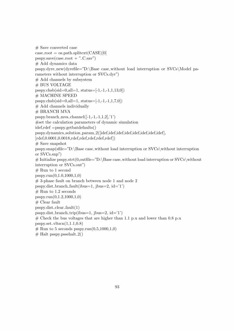
# Save converted casecase root = os.path.splitext(CASE)[0]psspy.save(case root + ” C.sav”)# Add dynamics datapsspy.dyre new(dyrefile=”D:\Base case without load interruption or SVCs\Model pa-rameters without interruption or SVCs.dyr”)# Add channels by subsystem# BUS VOLTAGEpsspy.chsb(sid=0,all=1, status=[-1,-1,-1,1,13,0])# MACHINE SPEEDpsspy.chsb(sid=0,all=1, status=[-1,-1,-1,1,7,0])# Add channels individually# BRANCH MVApsspy.branch mva channel([-1,-1,-1,1,2],’1’)#set the calculation parameters of dynamic simulationidef,rdef =psspy.getbatdefaults()psspy.dynamics solution param 2([idef,idef,idef,idef,idef,idef,idef,idef],[rdef,0.0001,0.0018,rdef,rdef,rdef,rdef,rdef])# Save snapshotpsspy.snap(sfile=”D:\Base case without load interruption or SVCs\without interruptionor SVCs.snp”)# Initialize psspy.strt(0,outfile=”D:\Base case without load interruption or SVCs\withoutinterruption or SVCs.out”)# Run to 1 secondpsspy.run(0,1.0,1000,1,0)# 3-phase fault on branch between node 1 and node 2psspy.dist branch fault(ibus=1, jbus=2, id=’1’)# Run to 1.2 secondspsspy.run(0,1.2,1000,1,0)# Clear faultpsspy.dist clear fault(1)psspy.dist branch trip(ibus=1, jbus=2, id=’1’)# Check the bus voltages that are higher than 1.1 p.u and lower than 0.8 p.upsspy.set vltscn(1,1.1,0.8)# Run to 5 seconds psspy.run(0,5,1000,1,0)# Halt psspy.pssehalt 2()

93

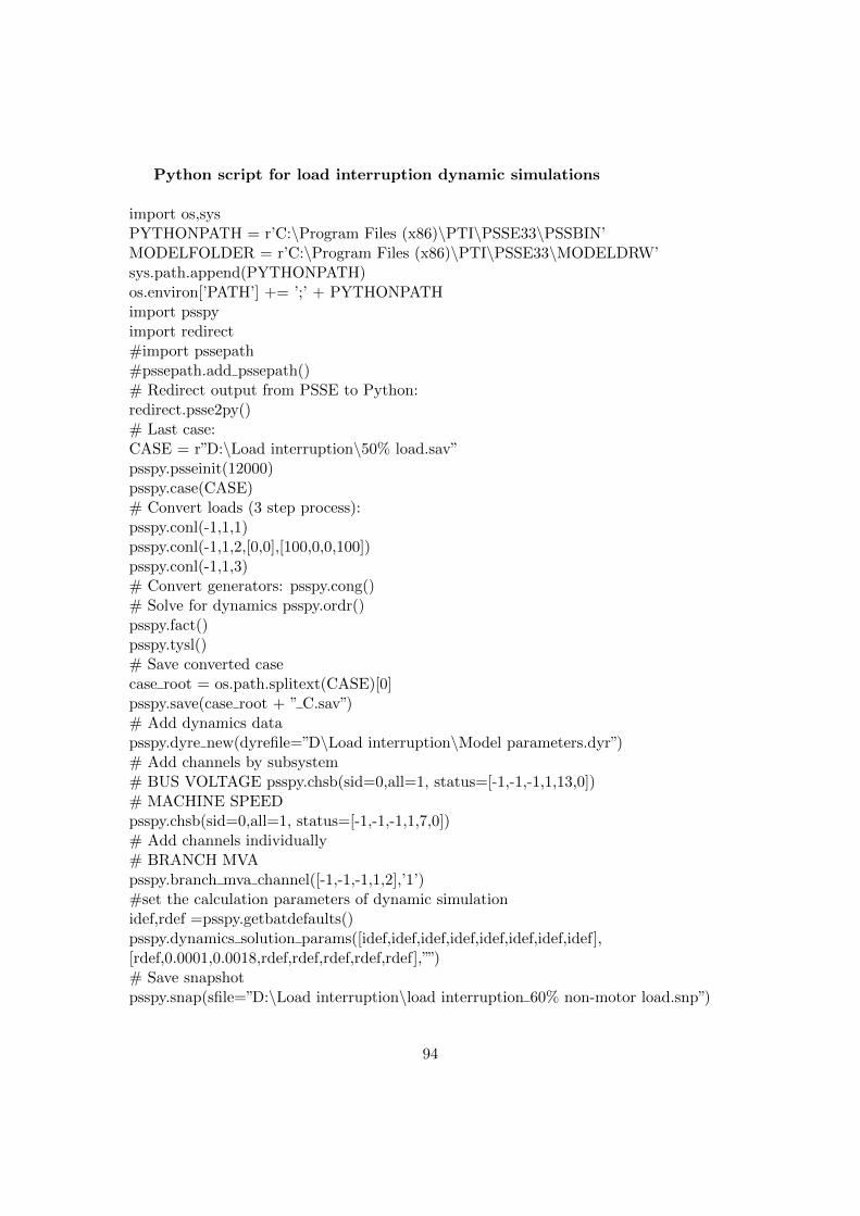
Python script for load interruption dynamic simulations

import os,sysPYTHONPATH = r’C:\Program Files (x86)\PTI\PSSE33\PSSBIN’MODELFOLDER = r’C:\Program Files (x86)\PTI\PSSE33\MODELDRW’sys.path.append(PYTHONPATH)os.environ[’PATH’] += ’;’ + PYTHONPATHimport psspyimport redirect#import pssepath#pssepath.add pssepath()# Redirect output from PSSE to Python:redirect.psse2py()# Last case:CASE = r”D:\Load interruption\50% load.sav”psspy.psseinit(12000)psspy.case(CASE)# Convert loads (3 step process):psspy.conl(-1,1,1)psspy.conl(-1,1,2,[0,0],[100,0,0,100])psspy.conl(-1,1,3)# Convert generators: psspy.cong()# Solve for dynamics psspy.ordr()psspy.fact()psspy.tysl()# Save converted casecase root = os.path.splitext(CASE)[0]psspy.save(case root + ” C.sav”)# Add dynamics datapsspy.dyre new(dyrefile=”D\Load interruption\Model parameters.dyr”)# Add channels by subsystem# BUS VOLTAGE psspy.chsb(sid=0,all=1, status=[-1,-1,-1,1,13,0])# MACHINE SPEEDpsspy.chsb(sid=0,all=1, status=[-1,-1,-1,1,7,0])# Add channels individually# BRANCH MVApsspy.branch mva channel([-1,-1,-1,1,2],’1’)#set the calculation parameters of dynamic simulationidef,rdef =psspy.getbatdefaults()psspy.dynamics solution params([idef,idef,idef,idef,idef,idef,idef,idef],[rdef,0.0001,0.0018,rdef,rdef,rdef,rdef,rdef],””)# Save snapshotpsspy.snap(sfile=”D:\Load interruption\load interruption 60% non-motor load.snp”)

94

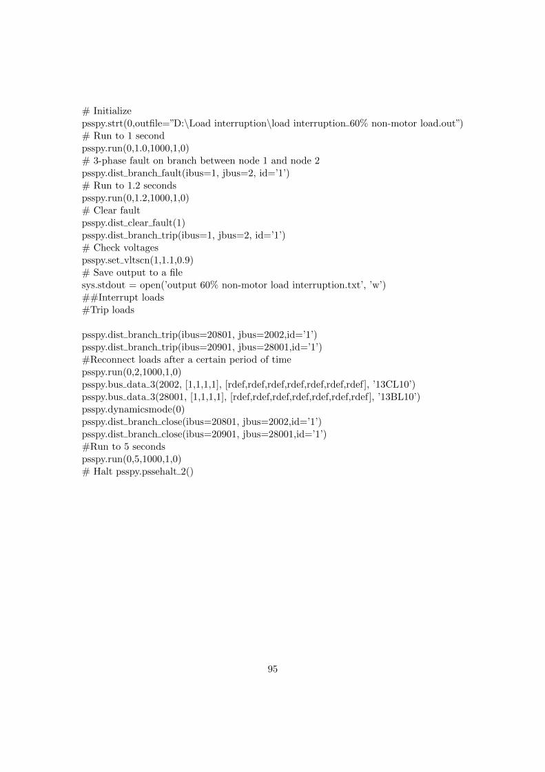
# Initializepsspy.strt(0,outfile=”D:\Load interruption\load interruption 60% non-motor load.out”)# Run to 1 secondpsspy.run(0,1.0,1000,1,0)# 3-phase fault on branch between node 1 and node 2psspy.dist branch fault(ibus=1, jbus=2, id=’1’)# Run to 1.2 secondspsspy.run(0,1.2,1000,1,0)# Clear faultpsspy.dist clear fault(1)psspy.dist branch trip(ibus=1, jbus=2, id=’1’)# Check voltagespsspy.set vltscn(1,1.1,0.9)# Save output to a filesys.stdout = open(’output 60% non-motor load interruption.txt’, ’w’)##Interrupt loads#Trip loads

psspy.dist branch trip(ibus=20801, jbus=2002,id=’1’)psspy.dist branch trip(ibus=20901, jbus=28001,id=’1’)#Reconnect loads after a certain period of timepsspy.run(0,2,1000,1,0)psspy.bus data 3(2002, [1,1,1,1], [rdef,rdef,rdef,rdef,rdef,rdef,rdef], ’13CL10’)psspy.bus data 3(28001, [1,1,1,1], [rdef,rdef,rdef,rdef,rdef,rdef,rdef], ’13BL10’)psspy.dynamicsmode(0)psspy.dist branch close(ibus=20801, jbus=2002,id=’1’)psspy.dist branch close(ibus=20901, jbus=28001,id=’1’)#Run to 5 secondspsspy.run(0,5,1000,1,0)# Halt psspy.pssehalt 2()

95

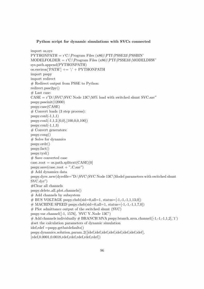
Python script for dynamic simulations with SVCs connected

import os,sysPYTHONPATH = r’C:\Program Files (x86)\PTI\PSSE33\PSSBIN’MODELFOLDER = r’C:\Program Files (x86)\PTI\PSSE33\MODELDRW’sys.path.append(PYTHONPATH)os.environ[’PATH’] += ’;’ + PYTHONPATHimport psspyimport redirect# Redirect output from PSSE to Python:redirect.psse2py()# Last case:CASE = r”D:\SVC\SVC Node 13C\50% load with switched shunt SVC.sav”psspy.psseinit(12000)psspy.case(CASE)# Convert loads (3 step process):psspy.conl(-1,1,1)psspy.conl(-1,1,2,[0,0],[100,0,0,100])psspy.conl(-1,1,3)# Convert generators:psspy.cong()# Solve for dynamicspsspy.ordr()psspy.fact()psspy.tysl()# Save converted casecase root = os.path.splitext(CASE)[0]psspy.save(case root + ” C.sav”)# Add dynamics datapsspy.dyre new(dyrefile=”D:\SVC\SVC Node 13C\Model parameters with switched shuntSVC.dyr”)#Clear all channelspsspy.delete all plot channels()# Add channels by subsystem# BUS VOLTAGE psspy.chsb(sid=0,all=1, status=[-1,-1,-1,1,13,0])# MACHINE SPEED psspy.chsb(sid=0,all=1, status=[-1,-1,-1,1,7,0])# Plot admittance output of the switched shunt (SVC)psspy.var channel([-1, 1576], ’SVC Y Node 13C’)# Add channels individually # BRANCH MVA psspy.branch mva channel([-1,-1,-1,1,2],’1’)#set the calculation parameters of dynamic simulationidef,rdef =psspy.getbatdefaults()psspy.dynamics solution param 2([idef,idef,idef,idef,idef,idef,idef,idef],[rdef,0.0001,0.0018,rdef,rdef,rdef,rdef,rdef])

96

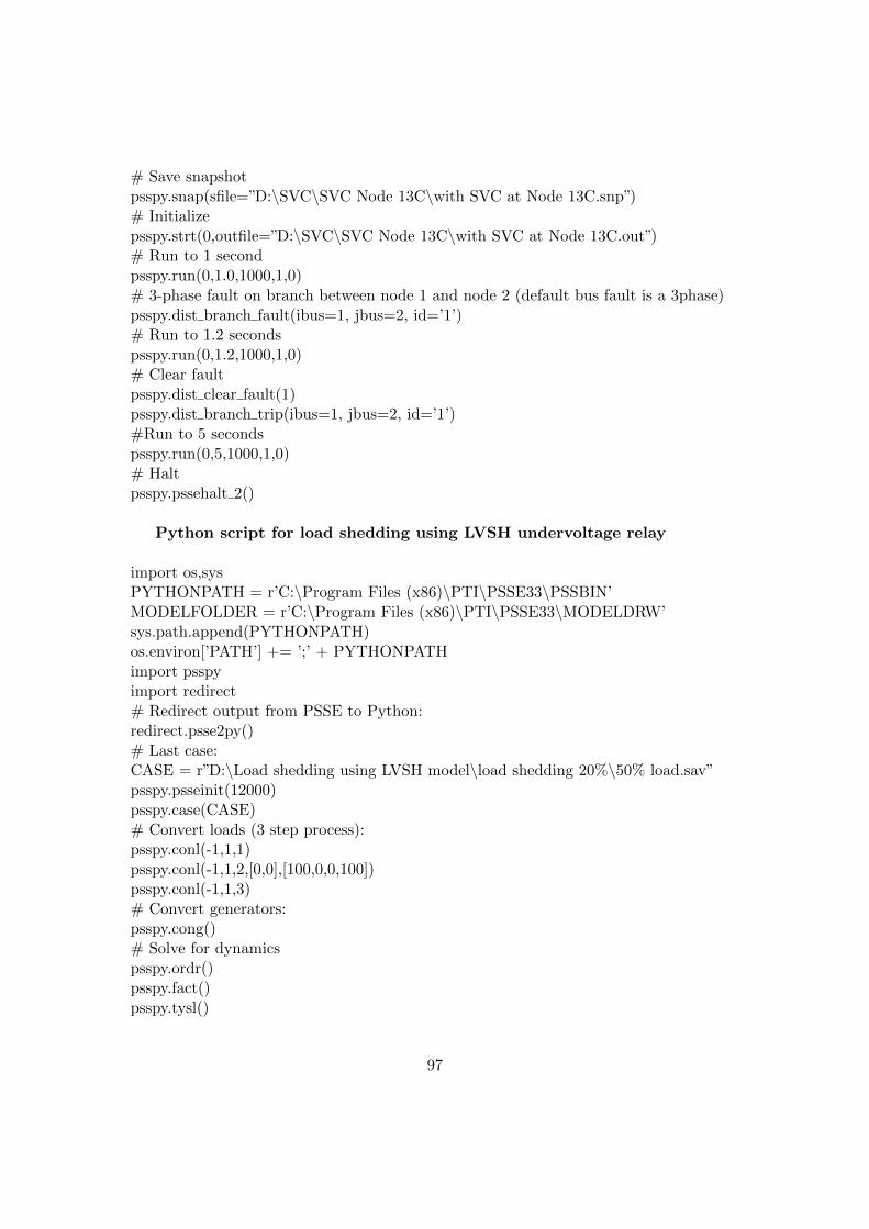
# Save snapshotpsspy.snap(sfile=”D:\SVC\SVC Node 13C\with SVC at Node 13C.snp”)# Initializepsspy.strt(0,outfile=”D:\SVC\SVC Node 13C\with SVC at Node 13C.out”)# Run to 1 secondpsspy.run(0,1.0,1000,1,0)# 3-phase fault on branch between node 1 and node 2 (default bus fault is a 3phase)psspy.dist branch fault(ibus=1, jbus=2, id=’1’)# Run to 1.2 secondspsspy.run(0,1.2,1000,1,0)# Clear faultpsspy.dist clear fault(1)psspy.dist branch trip(ibus=1, jbus=2, id=’1’)#Run to 5 secondspsspy.run(0,5,1000,1,0)# Haltpsspy.pssehalt 2()

Python script for load shedding using LVSH undervoltage relay

import os,sysPYTHONPATH = r’C:\Program Files (x86)\PTI\PSSE33\PSSBIN’MODELFOLDER = r’C:\Program Files (x86)\PTI\PSSE33\MODELDRW’sys.path.append(PYTHONPATH)os.environ[’PATH’] += ’;’ + PYTHONPATHimport psspyimport redirect# Redirect output from PSSE to Python:redirect.psse2py()# Last case:CASE = r”D:\Load shedding using LVSH model\load shedding 20%\50% load.sav”psspy.psseinit(12000)psspy.case(CASE)# Convert loads (3 step process):psspy.conl(-1,1,1)psspy.conl(-1,1,2,[0,0],[100,0,0,100])psspy.conl(-1,1,3)# Convert generators:psspy.cong()# Solve for dynamicspsspy.ordr()psspy.fact()psspy.tysl()

97

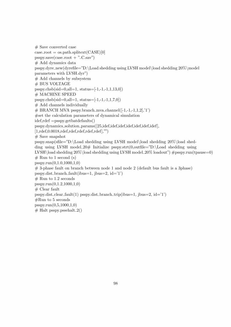
# Save converted casecase root = os.path.splitext(CASE)[0]psspy.save(case root + ” C.sav”)# Add dynamics datapsspy.dyre new(dyrefile=”D:\Load shedding using LVSH model\load shedding 20%\modelparameters with LVSH.dyr”)# Add channels by subsystem# BUS VOLTAGEpsspy.chsb(sid=0,all=1, status=[-1,-1,-1,1,13,0])# MACHINE SPEEDpsspy.chsb(sid=0,all=1, status=[-1,-1,-1,1,7,0])# Add channels individually# BRANCH MVA psspy.branch mva channel([-1,-1,-1,1,2],’1’)#set the calculation parameters of dynamical simulationidef,rdef =psspy.getbatdefaults()psspy.dynamics solution params([25,idef,idef,idef,idef,idef,idef,idef],[1,rdef,0.0018,rdef,rdef,rdef,rdef,rdef],””)# Save snapshotpsspy.snap(sfile=”D:\Load shedding using LVSH model\load shedding 20%\load shed-ding using LVSH model 20# Initialize psspy.strt(0,outfile=”D:\Load shedding usingLVSH\load shedding 20%\load shedding using LVSH model 20% loadout”) #psspy.run(tpause=0)# Run to 1 second (s)psspy.run(0,1.0,1000,1,0)# 3-phase fault on branch between node 1 and node 2 (default bus fault is a 3phase)psspy.dist branch fault(ibus=1, jbus=2, id=’1’)# Run to 1.2 secondspsspy.run(0,1.2,1000,1,0)# Clear faultpsspy.dist clear fault(1) psspy.dist branch trip(ibus=1, jbus=2, id=’1’)#Run to 5 secondspsspy.run(0,5,1000,1,0)# Halt psspy.pssehalt 2()

98