Investigation of two-phase microchannel flow and

phase equilibria in micro cells

for applications to enhanced oil recovery

by

Hooman Foroughi

A thesis submitted in conformity with the requirements for the degree of Doctor of Philosophy

Graduate Department of Chemical Engineering & Applied Chemistry University of Toronto

© Copyright by Hooman Foroughi 2012

ii

Investigation of two-phase microchannel flow and phase

equilibria in micro cells for applications in enhanced oil recovery

Hooman Foroughi

Doctor of Philosophy

Graduate Department of Chemical Engineering & Applied Chemistry

University of Toronto

2012

Abstract

The viscous oil-water hydrodynamics in a microchannel and phase equilibria of heavy oil

and carbon dioxide gas have been investigated in connection with the enhanced recovery of

heavy oil from petroleum reservoirs.

The oil-water flow was studied in a circular microchannel made of fused silica with an

I.D. of 250 µm. The viscosity of the silicone oil (863 mPa.sec) was close to that of the gas-

saturated heavy oil in reservoirs. The channel was always initially filled with the oil. Two

different sets of experiments were conducted: continuous oil-water flow and immiscible

displacement of oil by water. For the case of continuous water and oil injection, different types

of liquid-liquid flow patterns were identified and a flow pattern map was developed based on

Reynolds, Capillary and Weber numbers. Also, a simple correlation for pressure drop of the two

phase system was developed.

In the immiscible displacement experiments, the water initially formed a core-annular

flow pattern, i.e. a water core surrounded by a viscous oil film. The initially symmetric flow

iii

became asymmetric with time as the water core shifted off centre and also the waves at the oil-

water interface became asymmetric. A linear stability analysis for core-annular flow was also

performed. A characteristic equation which predicts the growth rate of perturbations as a

function of the core radius, Reynolds number, and viscosity and density ratios of the two phases

was developed.

Also, two micro cells for gas solubility measurements in oils were designed and

constructed. The blind cell had an internal volume of less than 2 ml and the micro glass cell had

a volume less than 100 µl. By minimizing the cell volume, measurements could be made more

quickly. The CO2 solubility was determined in bitumen and ashphaltene-free bitumen samples to

show that ashphaltene has a negligible effect on CO2 solubility.

iv

Acknowledgments

I would like to thank my supervisor, Prof. Masahiro Kawaji, and my labmates, Mehrrad,

Alireza, Dan and Kausik, for all their help. The committee members, Prof. Edgar Acosta, Prof.

Axel Guenther, Prof. Ramin Franood, and Prof. Khellil Sefiane, kindly provided me with their

insightful comments during my PhD program. I had helpful discussions with Prof. Charles Ward,

Prof. Arun Ramchandran and Prof. Naser Ashgriz. My special thanks to my family and friends,

Alireza, Sofia, Leila, Maryam, Pooya, Nima, and Hadi for their support.

v

Table of Contents

Acknowledgments .......................................................................................................................... iv

Table of Contents ............................................................................................................................ v

List of Tables ................................................................................................................................. ix

List of Figures ................................................................................................................................ x

List of Appendices ...................................................................................................................... xiv

Nomenclature ............................................................................................................................... xv

Chapter 1: Introduction ................................................................................................................... 1

1.1 Viscous oil-water flows in a microchannel initially saturated with oil: flow patterns

and pressure drop characteristics ........................................................................................ 3

1.2 Immiscible displacement of oil by water in a microchannel: asymmetric flow behavior

and stability analysis ........................................................................................................... 6

1.3 Gas solubility measurements by using micro-cells .............................................................. 7

Chapter 2: Viscous oil-water flows in a microchannel initially saturated with oil: flow

patterns and pressure drop characteristics ................................................................................ 10

2.1 Experimental details ........................................................................................................... 10

2.1.1 Materials ................................................................................................................. 10

2.1.2 Experimental facility ................................................................................................ 11

2.1.2.1 Continuous liquid injection ....................................................................... 11

2.1.2.2 Fluid injection section ............................................................................... 11

2.1.2.3 Pressure Drop and Flow Rate Measurements……………………….......................12

2.1.2.4 Image capture ............................................................................................ 13

2.2 Results and discussion ...................................................................................................... 14

2.2.1 Flow patterns ........................................................................................................... 14

2.2.2 Pressure Drop Measurements and Analysis for Slug, Annular and Annular-

Droplet Flows ........................................................................................................ 25

vi

Chapter 3: Immiscible displacement of oil by water in a microchannel: asymmetric flow

behaviour and non-linear stability analysis .............................................................................. 36

3.1. Experimental details .......................................................................................................... 36

3.1.1 Materials .................................................................................................................. 36

3.1.2 Experimental Facility ............................................................................................... 37

3.2. Flow Behaviour ................................................................................................................. 38

3.3. Stability analysis ............................................................................................................... 51

Chapter 4: A Miniature Cell for Gas Solubility Measurements in Oils and Bitumen .................. 62

4.1 Experimental Details .......................................................................................................... 62

4.1.1 Materials .................................................................................................................. 62

4.2 Experimental apparatus ...................................................................................................... 64

4.2.1 Solubility cell ........................................................................................................... 65

4.2.2. Pre-injection Cell .................................................................................................... 67

4.3. Experimental Procedure .................................................................................................... 68

4.3.1. Step 1: Liquid Injection into the Solubility Cell ..................................................... 68

4.3.2. Step 2: Gas Injection ............................................................................................... 70

4.3.2.1. Step 2-1: Gas Injection into the Pre-injection Cell .................................. 70

4.3.2.2. Step 2-2: Gas Injection from Pre-injection Cell into Solubility Cell ....... 71

4.3.3. Step 3: Solubility Measurements at 60 °C ............................................................. 71

4.3.4. Steps 4&5: Solubility Measurements at 35 °C and 22 °C ...................................... 73

4.3.5. Step 6: Changing the Cell Temperature to Room Temperature for Next Gas

Injection ................................................................................................................ 73

4.4. Results and Discussion ...................................................................................................... 74

4.5 Effect of gas dissolution on flow stability .......................................................................... 82

Chapter 5: Design of a micro glass cell apparatus for pure gas-nonvolatile liquid phase

behavior study .......................................................................................................................... 85

5-1) Experimental details ......................................................................................................... 85

vii

5-1-1) Materials ................................................................................................................ 85

5-1-2) Experimental apparatus .......................................................................................... 86

5-1-2-1) Micro cell ................................................................................................ 87

5-1-2-2) Gas line ................................................................................................... 88

5-1-2-3) Liquid line ............................................................................................... 89

5-1-3) Experimental procedure for systems with low viscosity liquids ........................... 89

5-1-3-1) Vacuuming the cell ................................................................................. 89

5-1-3-2) Gas injection into the cell ....................................................................... 90

5-1-3-3) Liquid injection into the cell ................................................................... 90

5-1-3-4) Temperature adjustment ......................................................................... 92

5-1-3-5) Mixing and reaching equilibrium conditions .......................................... 93

5-1-4) Experimental procedure for systems with highly viscous liquids ......................... 95

5-1-4-1) Manual bitumen injection ....................................................................... 95

5-1-4-2) Gas injection ........................................................................................... 96

5-1-4-3) Mercury injection ................................................................................... 97

5-2) Calculating reference CO2 solubility values in water from Henry’s law ......................... 98

5-3) Experimental results ......................................................................................................... 99

5-4) Error analysis .................................................................................................................. 101

5-4-1) Error due to the uncertainty in temperature and pressure measurements ............ 102

5-4-2) Error due to neglecting the liquid vapor pressure ................................................ 102

5-4-3) Error due to neglecting the gas diffusion through the needle .............................. 103

Chapter 6: Conclusions ............................................................................................................... 107

6.1. Viscous oil-water two phase flow in a microchannel .............................................. 107

6.2. Immiscible displacement of oil by water in a microchannel: asymmetric flow

behavior and stability analysis ............................................................................ 108

6.3. A miniature blind cell for solubility measurements ................................................. 109

viii

6.4. A micro glass cell for solubility measurements ....................................................... 109

References ................................................................................................................................... 111

Appendix I: Non-linear Stability analysis for core annular flow ................................................ 120

ix

List of Tables

Table 2-1. Constants C1 - C4 in Eqs. 7 and 8 for the present and Salim et al.’s (2008) pressure

drop data. .................................................................................................................................. 28

Table 3-1. Test conditions. ............................................................................................................ 39

Table 3-2. The initial ( a ) and last symmetric ( z ) wavelengths and wave speed. The

experimental values are compared with the results of the non-linear ( 1f ) and linear ( 2f )

analysis………………….. ....................................................................................................... 44

Table 4-1. SARA analysis of bitumen samples. .......................................................................... 64

Table 4-2. The effect of gas saturation on viscosity of Peace River bitumen............................... 83

x

List of Figures

Figure 1-1: Schematic of the CO2 and water injections into an oil reservoir. ................................ 3

Figure 2-1: Schematic of experimental apparatus ....................................................................... 12

Fig. 2-2. Schematic of injection section ........................................................................................ 13

Fig. 2-3. Effect of optical correction: a) without optical correction, b) with optical correction ... 14

Fig. 2-4. Flows in the microchannel injection section: a) Single-phase oil flow (QO=13

μl/min); b) Plug flow (QO=13 μl/min, QW=15 μl/min); c) Annular flow (QO=13 μl/min,

QW=48 μl/min); d) Annular flow (QO=22 μl/min, QW=70 μl/min). ......................................... 17

Fig. 2-5. Flow patterns observed in viscous oil-water flow in a microchannel initially filled

with oil: a) Droplet flow - water droplets in continuous oil phase (QO=13 μl/min, QW=2

μl/min); b) Plug Flow (QO=46 μl/min and QW=110 μl/min); c) Slug flow (QO=46 μl/min,

QW=225 μl/min); d & e) Annular flow with sausage-shaped interfacial deformations

(QO=46 μl/min, QW=530 μl/min); and f) Annular-droplet flow with smooth oil-water

interface (QO=46 μl/min and QW=1125 μl/min); g) Annular-droplet flow with wavy oil-

water interface (QO=46 μl/min, QW=2135 μl/min). ................................................................. 18

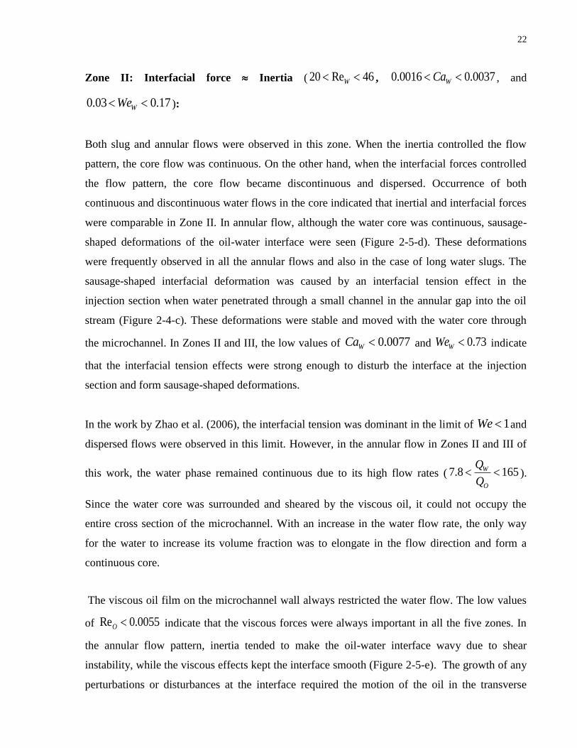
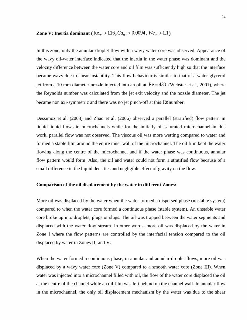
Fig. 2-6. Flow pattern map for silicone oil-water flow in a 250 μm microchannel initially

saturated with oil. The solid lines indicate the flow pattern transition boundaries. ................. 21

Fig. 2-7. Pressure drop data for silicone oil-water flow in a microchannel. The constants in

Eq. 8 are 276483 C and 5673434 C . ................................................................................... 29

Fig. 2-8. Prediction of Salim et al. (2008)’s pressure drop data for a glass microchannel by

Eq. 8 with 1453 C and 14704 C . ...................................................................................... 30

Fig. 2-9. Prediction of Salim et al. (2008)’s pressure drop data for a quartz microchannel by

Eq. 8 with 1123 C and 11144 C . ....................................................................................... 31

Fig. 2-10. Linear variation of the water two-phase friction multiplier,2

W , with Lockhart-

Martinelli parameter, 2 .......................................................................................................... 34

Fig. 2-11. Linear variation of the oil two-phase friction multiplier, 2

O , with the inverse of

the Lockhart-Martinelli parameter, 2

1

. ................................................................................ 35

Fig. 3-1. A schematic of the experimental apparatus. ................................................................... 38

xi

Fig. 3-2. Flow patterns at 5

4.8 10wi

Ca

and 39 10wCa observed in the middle of the

channel (top view) at different times from the start of the water injection.: a) at t=0 sec,

the channel was filled with oil; b) at t=50.7 sec, the water finger was displacing the oil at

the core; c) at t=53.3 sec, the oil film was left evenly on the channel wall and the oil-water

interface was smooth; d-1) at t=95.5 sec, symmetric perturbations formed at the interface;

d-2) at t=102.5 sec, the wavelength increased; e) at t=104.2, the water core shifted from

the centre and the flow became asymmetric; f) at 147.8 sec and g) at t=308.0, the water

core touched one side of the channel; h) at t=550 sec, the oil was completely displaced. ...... 40

Fig. 3-3. The initial water core thickness: the comparison of the experimental results with

Equation 4…………. ............................................................................................................... 41

Fig. 3-4. The water finger at 62 10wiCa observed in the middle of the channel, 714 sec after

the start of the water injection. The oil film on the channel wall is too thin to be observed…42

Fig. 3-5. The variation of the pressure at the channel inlet with time. ......................................... 44

Fig. 3-6. The water core fluctuation between the sides of the channel at 23.4 10wCa , a)

at 29.2 sec; b) at 30.2 sec; c) 33.4 sec. ..................................................................................... 46

Fig. 3-7. Flow patterns at 54.8 10wiCa and 39 10wCa , symmetric flow became

asymmetric: a) at 102.0 sec; b) at 102.6 sec; c) at 103.2 sec. .................................................. 47

Fig. 3-8. The variation of the maximum water core radius with time. ......................................... 48

Fig. 3-9. The variation of the maximum oil film thicknesses on opposite sides of the channel

with time…............................................................................................................................... 49

Fig. 3-10. A stable water core broke up into droplets after the flow was stopped: a)

asymmetric flow at 23.2 10wCa ; b) at 180 sec after the flow was stopped; c) at 740

sec after the flow was stopped. ................................................................................................ 51

Fig. 3-11. Dimensionless growth rate, , vs. dimensionless wave number,2

k

, at

1.03, 0.8, 0.0012,ol a m *Re 0.007 , 0.8wWe and 53 10oWe : the system

predicted by the non-linear analysis is more stable compared to the one predicted by the

linear analysis. .......................................................................................................................... 58

Fig. 3-12. The ratio of the fastest growing wavelength to the water core radius vs. water

Reynolds number. The results of the non-linear analysis (Eq. 29), linear analysis (Eq. 33),

and the last symmetric wavelength in experiments ( z ) are compared: a) Experimental

results are presented based on average velocities; b) Experimental results are presented

based on interfacial wave speed. The values of the water core radius in Equation 29 are

calculated by Equation 4. ......................................................................................................... 60

Fig. 4-1. Density of bitumen samples and maltene extracted from sample 1 vs. temperature. .... 63

xii

Fig. 4-2. Schematic of the experimental apparatus: 1) water bath 1 (WB1), 2) thermocouple,

3) solubility cell, 4) magnetic mixer, 5) rotating magnetic field, 6) T-junction, 7) pressure

transducer 1 (P1), 8) micro-valve 1 (V1), 9) pre-injection cell, 10) pressure transducer 2

(P2), 11) micro-valve 2 (V2), 12) purge valve, 13) gas regulator, 14) CO2 gas cylinder, 15)

data acquisition system, 16) water bath 2 (WB2), 17) computer. ............................................ 66

Fig. 4-3. Schematic of the solubility cell: 1) plug, 2) compression fitting, 3) column end

fitting, 4) magnetic mixer, 5) equilibrium cell, 6) micro-tube, 7) T-junction, 8) micro-tube

connected to pressure transducer 1 (P1), 9) micro-tube connected to micro-valve 1 (V1). .... 67

Fig. 4-4. Summary of the experimental procedure for solubility measurements. ......................... 69

Fig. 4-5. Formation of a liquid film inside the solubility cell. ...................................................... 70

Fig. 4-6. Changes in pressure and temperature of the solubility cell with time…………………72

Fig. 4-7. Variation of CO2 gas solubility in bitumen with pressure at 22 °C compared with

solubility data reported by Mehrotra and Svrcek (1985b) for Peace River bitumen................ 76

Fig. 4-8. Variation of CO2 gas solubility in bitumen with pressure at 35 °C. .............................. 77

Fig. 4-9. Variation of CO2 gas solubility in bitumen with pressure at 60 °C compared with

solubility data reported by Mehrotra and Svrcek (1985b) for Peace River bitumen................ 78

Fig. 4-10. Variation of CO2 gas solubility in bitumen sample 1 and maltene extracted from

sample 1 with pressure at 22 °C. The recalculated solubility in maltene accounts for the

amount of ashphaltene removed. .............................................................................................. 79

Fig. 4-11. Variation of CO2 gas solubility in bitumen sample 1 and maltene extracted from

sample 1 with pressure at 35 °C. The recalculated solubility in maltene accounts for the

amount of ashphaltene removed. .............................................................................................. 80

Fig. 4-12. CO2 gas solubility data for bitumen sample 1 at 22 °C from three runs. ..................... 81

Fig. 4-13. The effect of swelling on CO2 solubility in bitumen sample 1. ................................... 82

Fig. 4-14. Maximum dimensionless growth rate predicted by linear stability analysis vs.

dimensionless wave number, 2

k

, at 1.03, 0.75,ol a and

*Re 0.007 . .................... 84

Figure 5-1. Schematic of the experimental apparatus consisting of three parts: the micro cell,

gas line, and liquid line. The schematic is not to scale. ........................................................... 86

Figure 5-2. The glass syringe used as the micro cell with a magnetic mixer and a bitumen plug

inside………………………………………………………………………………………………………………………..…88

xiii

Figure 5-3. Schematic of the gas line and the micro cell for gas injection process: a) The gas

has been injected into the cell at pressure Pginj.

and at room temperature; b) The valve V1

is closed and the gas line is vacuumed for the second time before the liquid injection. .......... 91

Figure 5-4. Schematic of the liquid line and the micro cell for liquid injection. The liquid is

injected at pressure Plinj.

which is higher than the pressure of the gas injection. ..................... 92

Figure 5-5. Pressure change in the cell in each step for the solubility measurement by the

pressure decay method. ............................................................................................................ 93

Fig. 5-6. The micro cell for CO2 solubility measurements in bitumen: bitumen, CO2, and

mercury are injected into the cell before the start of the mixing. ............................................ 96

Figure 5-7. The schematic of the solubility cell presented in Chapter 4. ..................................... 98

Figure 5-8. CO2 solubility in water variation with pressure at temperatures of 31, 35, 40, and

50 oC. The solubility values measured in this study are compared with the reference values

(Perry et al., 1997) and the values calculated from Henry’s law (Equation 8). ..................... 100

Figure 5-9. CO2 solubility in bitumen vs. pressure at 22 oC. The experimental results of this

work are compared with the results presented in Chapter 4. ................................................. 101

Figure 5-10. The schematic of the gas diffusion problem through the needle. .......................... 105

Figure I-1. Schematic of core-annular flow. ............................................................................... 120

xiv

List of Appendices

Appendix I. Nonlinear stability analysis for core annular flow .................................................. 120

xv

Nomenclature

A constant

a water core radius

ao unperturbed water core radius

B constant

Bo Bond number

C constant (Chapter 2); molar concentration (Chapter 5)

Ca Capillary number

Dgl gas diffusion coefficient in liquid

D channel diameter

d water core diameter

f fugacity

G Gibbs energy

H enthalpy

h oil film thickness

k wave number (Chapter 3); Henry constant (Chapter 5)

L channel length (Chapter 2); needle length (Chapter 5)

xvi

l water to oil density ratio

M molecular weight

m water to oil viscosity ratio (Chapter 3); mass (Chapters 4 & 5)

N molar flux

n number of moles

P pressure

P1-P2 pressure transducers

P̂ solute partial pressure

Q volumetric flow rate

R channel radius (Chapter 3); gas constant (Chapter 5)

Re Reynolds number

r radius

S solubility (Chapter 4); entropy (Chapter 5)

T temperature

t time

V velocity (Chapters 2&3); volume (Chapters 4&5)

V1-V6 valves

xvii

U dimensionless velocity

W solubility

W*

characteristic velocity

We Weber number

x distance from the solubility cell

z flow direction

Greek symbols

α constant

β constant

εo oil to mixture volumetric flow rate ratio

η constant for microchannel property

λ dimensionless wavelength

µ viscosity

density

φ Lockhart-Martinelli friction multiplier

π pi constant

xviii

σ interfacial tension

χ Lockhart-Martinelli parameter

ω dimensionless frequency

Subscripts and superscripts

a first

eq. equilibrium

c critical

f fastest

i initial

inj. injection

G gas (Chapter 4)

g gas (Chapter 5)

L liquid (Chapter 4)

l liquid (Chapter 5)

max maximum

o oil

xix

TP two phase

w water

z last

* characteristic parameter (Chapter 3); reference state ( Chapter 5)

_ average

/ perturbations

1

Chapter 1

Introduction

To enhance oil recovery, immiscible liquids such as water are injected into petroleum reservoirs

in order to displace and push out oil towards the production wells (Figure 1-1). For recovery of

highly viscous oils, such as bitumen, miscible gases such as CO2 can be injected before the

immiscible (water) injection. The oil viscosity is significantly reduced as the gas is dissolved in

the oil, which increases the oil flow rate (Simon et al., 1965; Jacobs et al., 1980). Knowledge of

the oil-water flow characteristics and also gas solubility in oil is thus required to design and

optimize the enhanced oil recovery process.

In this study, the two-phase oil-water flow in a microchannel was investigated in connection with the

flow of oil and water in petroleum reservoirs. The viscosity of the oil (863 mPa.s) used in the

experiments was comparable to that of the gas saturated bitumen in reservoirs. The microchannel

diameter (250 µm) was in the range of the pore size of porous media in oil reservoirs. Although the

flow passages in petroleum reservoirs would be highly interconnected and not straight channels, the

present experiments were performed to gain a basic understanding of the hydrodynamics of viscous

oil-water in a well-defined microchannel geometry.

Before each experiment, the microchannel was always initially saturated with oil. Two separate sets

of experiments were performed to compare different flow conditions for oil recovery: in the first set

of experiments, oil and water were simultaneously injected into the initially oil-saturated

microchannel (Chapter 2). Different oil-water flow patterns were identified some of which have not

been reported in previous works, i.e. annular-droplet flow with a smooth or wavy interface. The

interfacial tension, inertia, and viscous forces which would control the flow pattern were compared

and a new flow pattern map was developed based on the dimensionless Capillary, Weber, and

Reynolds numbers. The amounts of the oil displaced by the water in different flow patterns were also

compared. The pressure drop data were collected and analyzed. A simple model was developed for

the oil-water two-phase pressure drop in initially oil saturated microchannels. It is shown that this

2

model is applicable to systems of oil-water flows with different oil viscosity and also with different

micorchannel geometries.

In the second set of experiments referred to as the immiscible oil displacement experiments, the

microchannel was filled with oil and then only water was injected into the channel to displace the oil

(Chapter 3). The asymmetric flow behavior observed with time in the immiscible displacement

experiments has not been reported in previous studies. The rates of the oil displacement under

different experimental conditions were compared. A suggestion is made that intermittent water

injection can improve the rate of oil recovery.

A linear stability analysis was also performed on core-annular flows. The water core remained

continuous in a stable system but tended to form a dispersed phase in an unstable system. This

analysis allows us to determine the sensitivity of the flow stability to different fluid properties such

as density and viscosity ratio of the two phases.

For gas solubility measurements in heavy oil (bitumen) samples, two micro cells were designed and

constructed: a miniature blind cell with a volume of less than 2 ml (Chapter 4) and a micro glass cell

with a volume less than 100 µl (Chapter 5). By minimizing the volume of the cell, the time required

for the system to reach equilibrium which could take up to weeks or months in previous designs

(Badamchi-Zadeh et al., 2009) was reduced to less than 90 minutes with the glass cell and less than

10 minutes with the blind cell. The CO2 solubility measurements in bitumen and asphaltene-free

bitumen were compared to find that ashphlatene had a negligible effect on CO2 solubility. Also, in

Chapter 4, the effect of gas dissolution on the flow stability is discussed based on the results of the

stability analysis presented in Chapter 3.

Although the motivation behind the microchannel flow study is to understand the water-oil flow

characteristics in petroleum reservoirs better, the discussion provided in Chapter 2 may be generally

applicable to liquid-liquid two-phase flows in microchannels for different applications. Also, the use

of the solubility cells described in Chapters 4 and 5 is not limited to gas-oil systems and these cells

can be used for a variety of gas-liquid mixtures.

3

Figure 1-1: Schematic of the CO2 and water injections into an oil reservoir.

1.1 Viscous oil-water flows in a microchannel initially saturated

with oil: flow patterns and pressure drop characteristics

Liquid-liquid flows are encountered in a wide range of applications in chemical engineering such

as microreactors and a lab-on-a-chip (Gunther et al., 2006), and petroleum engineering (Joseph et

al., 1997). Numerous investigations have been carried out on liquid-liquid flows in conventional

pipes with large hydraulic diameters. Many of these studies were performed in horizontal and

vertical pipes as reviewed by Joseph et al. (1997) and Ghosh et al. (2009). In microchannels with

hydraulic diameters of 50 – 500 µm, gas-liquid flows have been investigated extensively at the

University of Toronto (Kawahara et al., 2002; Chung and Kawaji, 2004; Chung et al., 2004;

Kawahara et al., 2005; Santos et al., 2010). In the case of liquid-liquid flows in microchannels,

many researchers have studied the formation of droplets in microfluidic devices (Thorsen et al.,

4

2001; Anna et al., 2003; Tice et al., 2003; Cramer et al., 2004; Garstecki et al., 2006; Tan et al.,

2008; Baroud et al., 2010), as well as the hydrodynamics and pressure drop of slug flow (Kashid

and Agar, 2007; Jovanovic et al., 2011). However, only few flow pattern maps have been

presented for liquid-liquid flows in microchannels (Zhao et al., 2006; Dessimoz et al., 2008;

Salim et al., 2008).

The liquid-liquid flow patterns in microchannels are known to be influenced by the fluid

properties including the wetting properties of the fluid and microchannel (Dreyfus et al., 2003;

Salim et al., 2008), the geometry and size of the channel and the injection section (Kashid and

Agar, 2007; Dessimoz et al., 2008) and the dominant forces which control the flow pattern (Zhao

et al., 2006; Dessimoz et al., 2008). Liquid-liquid flow patterns and pressure drop correlations

for microchannels, especially when one of the phases is highly viscous, however, have not been

very well understood yet.

Cramer et al. (2004) experimentally studied the formation of droplets in rectangular capillaries

by injecting the dispersed phase through a needle. Two different breakup mechanisms were

distinguished: dripping and jetting. In dripping, the droplets were formed close to the injection

section while in jetting the droplets were formed from an extended jet downstream. Guillot et al.

(2007) studied the stability of a jet in circular capillaries by performing a linear stability analysis.

A stable system formed a continuous jet regime and an unstable jet broke up into droplets. The

results of the stability analysis were presented based on the capillary number, viscosity ratio,

unperturbed jet diameter and flow rates.

Zhao et al. (2006) studied the flow of water and kerosene in a T-junction microchannel. They

observed different flow patterns and developed a flow pattern map based on a Weber number.

The flow pattern map was divided into three zones: the interfacial tension dominated zone, the

transition zone where inertia and interfacial tension were comparable, and the inertia dominated

zone. They also studied the mechanism of droplet and slug formation at the T-junction. Kashid

and Agar (2007) investigated the flow pattern, slug size, interfacial area, and pressure drop for

liquid-liquid slug flow in Y-junction mixing elements with various downstream capillaries. They

showed that the slug size and interfacial area would change with the Y-junction and capillary

dimensions. They also developed a theoretical model for predicting the pressure drop. The model

5

included individual terms for capillary pressure drop and hydrodynamic pressure drop. Dessimoz

et al. (2008) studied the flow pattern and mass transfer characteristics of water-toluene and

water-hexane flows in T-junction and Y-junction microchannels. They developed flow pattern

maps based on Reynolds and Capillary numbers and discussed how interfacial forces compete

with viscous forces to change the flow pattern from parallel to slug flow.

Salim et al. (2008) studied the oil-water flow patterns and pressure drops in micro T-junctions.

They used homogeneous flow and Lockhart-Martinelli correlations to interpret the measured

pressure drops. The flow patterns and pressure drop were found to depend on the type of the

fluid which was first injected into the channel and the channel material. Jovanovic et al. (2011)

studied the hydrodynamics and pressure drop of slug flow in circular microchannels. Two

pressure drop models were presented: a stagnant film model and moving film model. Both

models considered the formation of a thin film between slugs and the channel wall. They showed

that the film velocity could be neglected and the stagnant film model could be used to predict the

pressure drop data.

In the case of viscous liquid-liquid flows in microchannels, Cubaud and Mason (2006, 2007,

2008b, 2009) investigated the flow behaviour of miscible fluids. Regarding the flow of

immiscible liquids, they studied the flow of a viscous thread surrounded by a less viscous fluid in

square microchannels (Cubaud and Mason, 2008a). They developed a flow pattern map based on

the capillary number of each fluid and distinguished five different flow regimes: threading,

jetting, dripping, tubing, and displacement.

In Chapter 2, the flow patterns and pressure drop for a mixture of highly viscous oil with a

viscosity of 863 mPa.s and water flowing in a circular microchannel will be presented. The

channel was initially saturated with the oil, and then water and oil were injected into the

microchannel simultaneously. Video images of liquid-liquid flow patterns were analyzed to

develop a flow pattern map. The amounts of the oil displaced by the water in different flow

patterns were qualitatively compared. Also, pressure drop data were analyzed to develop a

simple pressure drop correlation applicable to slug, annular and annular-droplet flows in a

microchannel.

6

1.2 Immiscible displacement of oil by water in a microchannel:

asymmetric flow behavior and stability analysis

When a more viscous fluid is displaced by a less viscous fluid in a channel, the interface

between the two fluids forms a finger. While the finger moves, it leaves a film of the more

viscous fluid on the channel wall. This phenomenon is known as viscous fingering and was

studied for the first time by Saffman and Taylor in a Hele-Shaw cell (Saffman et al., 1958).

Viscous fingering frequently occurs in nature and in many engineering problems including the

immiscible displacement of oil in petroleum reservoirs. The past studies have usually been

conducted in Hele-Shaw cells or in microchannels to approximate the flow in petroleum

reservoirs (Homsy et al., 1987; Aul et al. 1990).

Viscous fingering has been studied extensively mainly to predict the thickness of the film

deposited on the channel wall. The phenomenon has been well documented in this regard and

some correlations have been developed for film thickness prediction (Bretherton et al., 1961;

Taylor et al., 1961; Park et al., 1984; Aussillous et al., 2000; Krechetnikov, 2005). However, the

thickness of the finger may not always match the predicted value and fluctuations in the finger

width have been reported (Moore et al., 2002). Perturbations at the interface were observed both

in experiments (McCloud et al., 1995; Torralba et al., 2006; Duclaux et al., 2006) and in

numerical simulations (Ledesma-Aguilar et al., 2005; Quevedo-Reyes, 2006). The stability of

the viscous finger is also an important phenomenon to study. An unstable finger breaks up into

droplets whereas a stable finger remains continuous and keeps growing (Aul, 1990).

In Chapter 3, we studied the displacement of viscous silicone oil by water in a

microchannel. The microchannel was initially saturated with oil and then only water was injected

into the channel to displace the oil. The focus of the previous studies has been more on the

motion of a viscous finger front. In the present work, we continued the immiscible displacement

experiments until the oil was completely displaced and the water occupied the entire

microchannel. The rates at which the oil was displaced by the water under different test

conditions were compared.

7

In the experiments, after the water finger had reached the channel outlet, the flow regime

changed from fingering to core-annular flow where the water core was surrounded by an oil film.

Although initially the flow regime was symmetric, the displacing water core shifted towards one

side of a channel and asymmetric perturbations were observed at the interface with time. To the

best of our knowledge, such flow behaviour has not been reported in previous works. Under

these experimental conditions, we have not observed any break up and droplet formation during

injection of water in the core. We will also discuss the stability of the displacing fluid based on

non-linear and linear stability analyses.

1.3 Gas solubility measurements by using micro-cells

Since heavy oil samples from different reservoirs have different physical properties, the gas

solubility in oil reservoirs should be measured for each production area (Mehrotra et al., 1985a,

1985b, & 1985c). Measuring the gas solubility in oil fractions and cuts would also be useful for

developing models to predict gas solubility in oil as a mixture (Mehrotra et al., 1986).

Methods used for gas solubility measurements in oil fall into two general categories: direct and

indirect methods. Direct methods require taking samples from gas-liquid mixtures at equilibrium

and measuring the amount of gas dissolved in each sample. Sampling introduces some

uncertainty and makes measurements difficult and relatively expensive. In contrast, indirect

methods do not involve any sampling which makes measurements more convenient. By using

indirect methods, measurements can be done at higher pressures and temperatures (Cai et al.,

2001).

The most commonly used indirect method is called the pressure decay method. This method was

first used by Riazi (1996) for measuring the solubility of methane in n-pentane. In this method,

gas solubility is calculated from pressure decay data. Pressure decays as a result of gas

dissolution in liquid. Finally, the gas-oil system reaches a constant pressure which shows that the

fluids in the cell are at equilibrium.

Measuring gas solubility in oils in conventional cells with large internal volumes is always

challenging. Reaching equilibrium conditions may take weeks to months (Badamchi-Zadeh et

8

al., 2009). The dissolution of gas into bitumen samples is a very slow process because of the

large internal cell volumes, relatively small gas-liquid interfacial area per unit volume, and slow

gas diffusion into the sample liquid (Upreti et al., 2000 & 2002). Having homogeneous and

uniform gas-liquid mixtures increases the mixing time due to the high viscosity of oils and

bitumen. Leakage of gas over a long period of time at high pressures is also a concern.

In contrast, experiments with gas-bitumen mixtures can be more easily conducted in a miniature

cell for the collection of solubility data. By minimizing the sample volume, complete mixing

would be achieved much faster. Also, the impact of accidental exposure to the gas is reduced, if

toxic gases such as hydrogen sulphide are used. Furthermore, a small cell can be more easily

sealed and experiments at high pressures and temperatures can be carried out. Unlike the

conventional cells, the components of a miniature cell are readily available and inexpensive.

In Chapter 4, a miniature stainless steel cell has been designed and constructed for gas solubility

measurements in oils and bitumen. The cell had an internal volume of 1.835 cc and only 0.4 cc

of an oil sample was required for each set of measurements. The cell alone could be operated at

pressures up to 42.7 MPa. In this cell, a large gas-liquid interfacial area was provided by

spreading the liquid as a film on the cell inner wall which helped establish phase equilibrium

sooner. The pressure decay method was used to evaluate the gas solubility in oil and bitumen

samples.

In each experiment, multiple gas injections were performed and gas solubility was measured at

different pressures. Also, after each gas injection, the solubility was measured at different

temperatures by changing the temperature of the solubility cell. In this way, a wide range of

solubility data could be collected at different temperatures and pressures with one time liquid

injection. The new technique was validated by measuring the CO2 solubility in bitumen and

ashphaltene-free bitumen samples from the Peace River area in Alberta, Canada.

In Chapter 5, a glass micro cell which uses an indirect method for phase behavior studies is

described. The apparatus can be used for the phase behavior study of pure gas and nonvolatile

liquid mixtures. A micro glass syringe with a volume of 100 µl is used as a constant volume cell.

Two different experimental procedures are developed for gas solubility measurements in low

9

viscous and high viscous liquids. The experimental procedure for the systems with low viscosity

liquids has been validated by measuring the solubility of CO2 in water. The cell pressure and the

volume of the gas phase were controlled by the volume of the water injected into the cell. Under

the experimental conditions tested in this study, the waiting time for the CO2-water system to

reach equilibrium was less than 8 minutes. The results are compared and found to be in a good

agreement with the available literature data and also with reference values calculated from

Henry’s law. Also, the experimental procedure proposed for the systems with highly viscous

liquids was tested by measuring the CO2 solubility in a bitumen sample from Peace River in

Alberta, Canada. The bitumen sample was about 3,000 times more viscous than water at 50 oC.

About a 90 minute mixing time was sufficient to bring the CO2-bitumen mixture to equilibrium.

10

Chapter 2

Viscous oil-water flows in a microchannel initially saturated with

oil: flow patterns and pressure drop characteristics

Immiscible viscous liquid-liquid two-phase flow patterns and pressure drop characteristics in a

circular microchannel have been investigated. Water and silicone oil with a dynamic viscosity of

863 mPa.s were injected into a fused silica microchannel with an inner diameter of 250 μm. As

the microchannel was initially filled with the silicone oil, an oil film was found to always form

and remain on the microchannel wall. Different flow patterns were observed and classified over

a wide range of water and oil flow rates. A flow pattern map is presented in terms of Re , Ca ,

and We numbers. Two-phase pressure drop data have also been collected and analyzed to

develop a simple correlation for slug, annular and annular-droplet flow patterns in terms of

superficial water and oil velocities.

2.1 Experimental details

2.1.1 Materials

The working fluids used in this study were de-ionized water and silicone oil from Sigma

Aldrich’s 200 fluid series. The viscosity and density of silicone oil were 863 mPa.s and 970

kg/m3 at 20 °C, respectively. The water-to-oil viscosity ratio was 0.0012, while the water-to-oil

density ratio was close to unity (=1.03). The oil’s surface tension and oil-water interfacial tension

were measured to be 21 mN/m and 43 mN/m at 20 °C, respectively.

A circular microchannel from Polymicro Technologies was used in the present experiments. The

microchannel made of fused silica was 7.0 cm long and had an inner diameter of 250 μm. The

contact angles of oil and water with the microchannel wall were 25° and 36°, respectively.

11

2.1.2 Experimental facility

2.1.2.1 Continuous liquid injection

If syringe pumps are used for liquid injection, the volume of the liquid injected into the channel

is limited to the volume of the syringe. Also, syringe pumps may not be forceful enough for

injecting highly viscous liquids. By using pneumatic pumps, liquids can be continuously injected

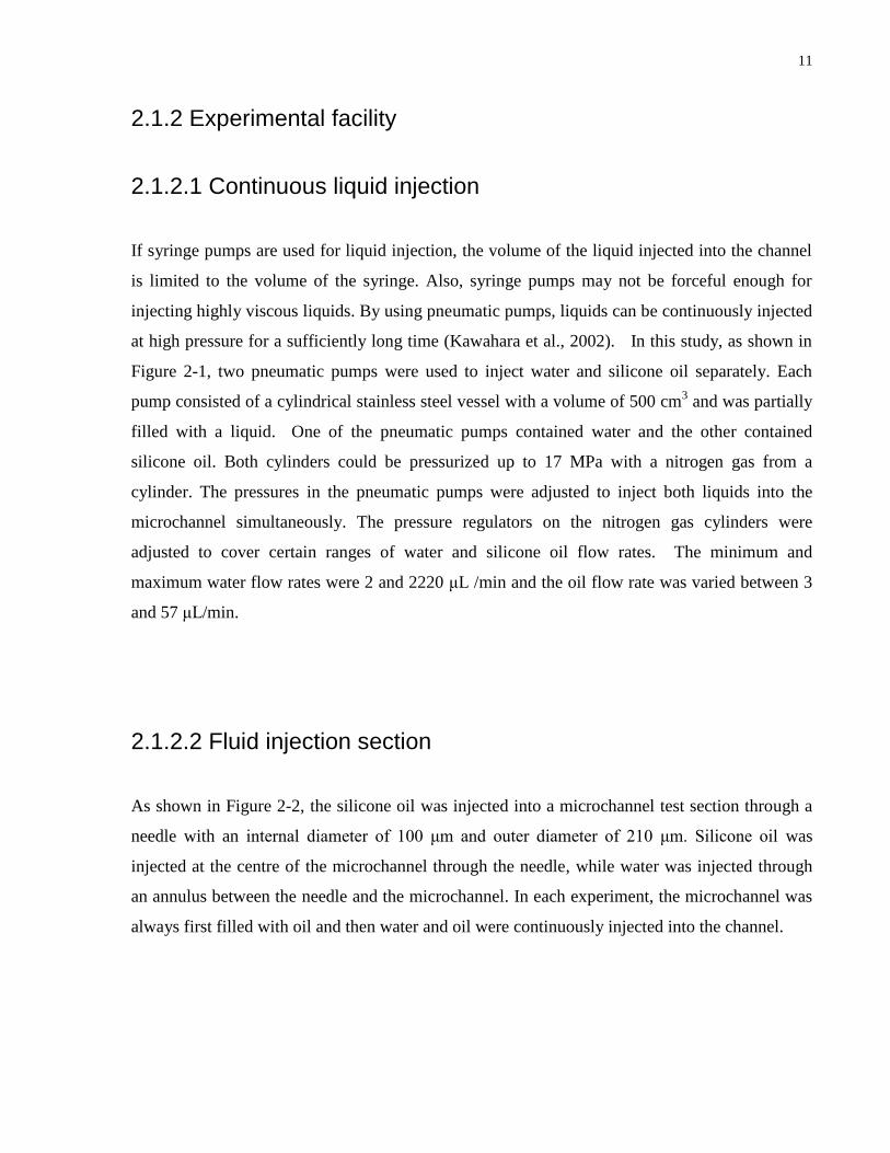
at high pressure for a sufficiently long time (Kawahara et al., 2002). In this study, as shown in

Figure 2-1, two pneumatic pumps were used to inject water and silicone oil separately. Each

pump consisted of a cylindrical stainless steel vessel with a volume of 500 cm3 and was partially

filled with a liquid. One of the pneumatic pumps contained water and the other contained

silicone oil. Both cylinders could be pressurized up to 17 MPa with a nitrogen gas from a

cylinder. The pressures in the pneumatic pumps were adjusted to inject both liquids into the

microchannel simultaneously. The pressure regulators on the nitrogen gas cylinders were

adjusted to cover certain ranges of water and silicone oil flow rates. The minimum and

maximum water flow rates were 2 and 2220 μL /min and the oil flow rate was varied between 3

and 57 μL/min.

2.1.2.2 Fluid injection section

As shown in Figure 2-2, the silicone oil was injected into a microchannel test section through a

needle with an internal diameter of 100 μm and outer diameter of 210 μm. Silicone oil was

injected at the centre of the microchannel through the needle, while water was injected through

an annulus between the needle and the microchannel. In each experiment, the microchannel was

always first filled with oil and then water and oil were continuously injected into the channel.

12

Figure 2-1: Schematic of experimental apparatus

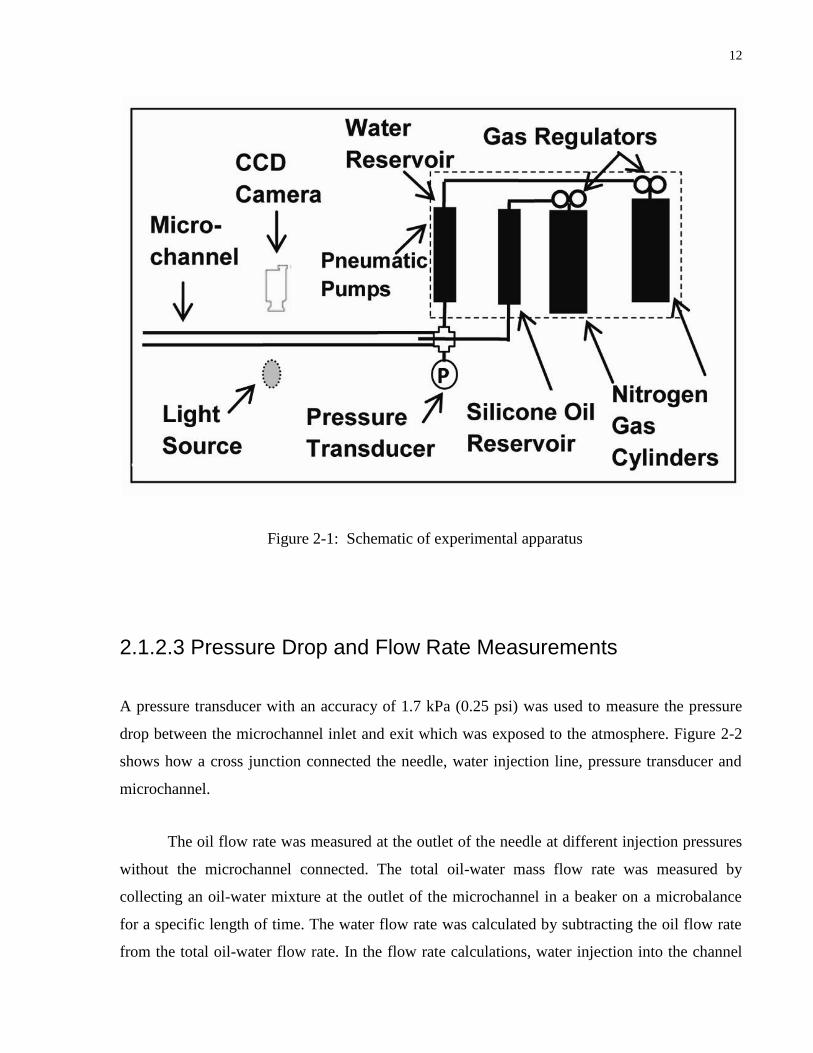
2.1.2.3 Pressure Drop and Flow Rate Measurements

A pressure transducer with an accuracy of 1.7 kPa (0.25 psi) was used to measure the pressure

drop between the microchannel inlet and exit which was exposed to the atmosphere. Figure 2-2

shows how a cross junction connected the needle, water injection line, pressure transducer and

microchannel.

The oil flow rate was measured at the outlet of the needle at different injection pressures

without the microchannel connected. The total oil-water mass flow rate was measured by

collecting an oil-water mixture at the outlet of the microchannel in a beaker on a microbalance

for a specific length of time. The water flow rate was calculated by subtracting the oil flow rate

from the total oil-water flow rate. In the flow rate calculations, water injection into the channel

13

was assumed to have a negligible effect on the single-phase flow rate of oil through the needle.

The oil reservoir was pressurized to a very high pressure for injecting the viscous oil through the

needle such that the pressure drop across the needle was much greater than that in the

microchannel at least by a factor of 10. To experimentally confirm this assumption, the oil-water

mixture was collected at the outlet of the microchannel for a long time until the volume of the oil

collected became measureable. The oil flow rates measured before and after connecting the

microchannel were compared. This experiment was repeated over a wide range of oil and water

flow rates and the results showed the maximum uncertainty of 7% in the oil flow rate.

Fig. 2-2. Schematic of injection section

2.1.2.4 Image capture

A high speed video camera was used to capture images of the water-silicone oil flow at a frame

rate of up to 125 frames per second. To minimize the entrance and exit effects on the flow

patterns observed, images were captured in the middle of the channel at 3.5 cm or 140 diameters

downstream of the tip of the needle used for water injection. Since a circular microchannel was

14

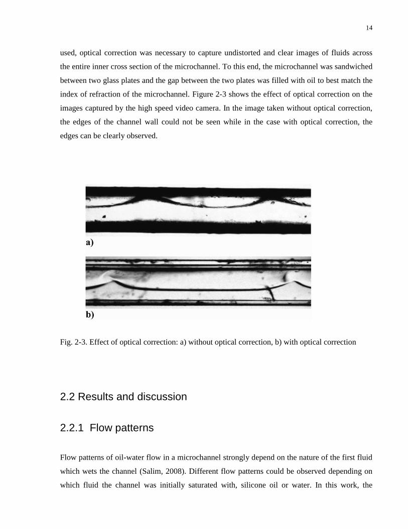
used, optical correction was necessary to capture undistorted and clear images of fluids across

the entire inner cross section of the microchannel. To this end, the microchannel was sandwiched

between two glass plates and the gap between the two plates was filled with oil to best match the

index of refraction of the microchannel. Figure 2-3 shows the effect of optical correction on the

images captured by the high speed video camera. In the image taken without optical correction,

the edges of the channel wall could not be seen while in the case with optical correction, the

edges can be clearly observed.

Fig. 2-3. Effect of optical correction: a) without optical correction, b) with optical correction

2.2 Results and discussion

2.2.1 Flow patterns

Flow patterns of oil-water flow in a microchannel strongly depend on the nature of the first fluid

which wets the channel (Salim, 2008). Different flow patterns could be observed depending on

which fluid the channel was initially saturated with, silicone oil or water. In this work, the

15

channel was always saturated with silicone oil initially by injecting only the silicone oil first at a

given flow rate. Then, water was injected into the microchannel at different flow rates while the

oil flow rate was kept constant.

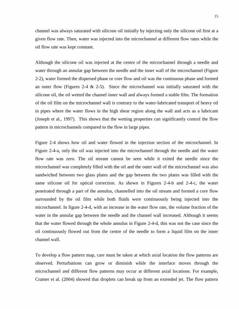
Although the silicone oil was injected at the centre of the microchannel through a needle and

water through an annular gap between the needle and the inner wall of the microchannel (Figure

2-2), water formed the dispersed phase or core flow and oil was the continuous phase and formed

an outer flow (Figures 2-4 & 2-5). Since the microchannel was initially saturated with the

silicone oil, the oil wetted the channel inner wall and always formed a stable film. The formation

of the oil film on the microchannel wall is contrary to the water-lubricated transport of heavy oil

in pipes where the water flows in the high shear region along the wall and acts as a lubricant

(Joseph et al., 1997). This shows that the wetting properties can significantly control the flow

pattern in microchannels compared to the flow in large pipes.

Figure 2-4 shows how oil and water flowed in the injection section of the microchannel. In

Figure 2-4-a, only the oil was injected into the microchannel through the needle and the water

flow rate was zero. The oil stream cannot be seen while it exited the needle since the

microchannel was completely filled with the oil and the outer wall of the microchannel was also

sandwiched between two glass plates and the gap between the two plates was filled with the

same silicone oil for optical correction. As shown in Figures 2-4-b and 2-4-c, the water

penetrated through a part of the annulus, channelled into the oil stream and formed a core flow

surrounded by the oil film while both fluids were continuously being injected into the

microchannel. In figure 2-4-d, with an increase in the water flow rate, the volume fraction of the

water in the annular gap between the needle and the channel wall increased. Although it seems

that the water flowed through the whole annulus in Figure 2-4-d, this was not the case since the

oil continuously flowed out from the centre of the needle to form a liquid film on the inner

channel wall.

To develop a flow pattern map, care must be taken at which axial location the flow patterns are

observed. Perturbations can grow or diminish while the interface moves through the

microchannel and different flow patterns may occur at different axial locations. For example,

Cramer et al. (2004) showed that droplets can break up from an extended jet. The flow pattern

16

before the break up can be considered as annular flow while after the break up the flow pattern

becomes droplet flow. Zhao et al. (2006) developed two different flow pattern maps: one at the

T-junction and the other further downstream in the microchannel. The chaotic thin striation flow

they observed at the T-junction eventually evolved to annular flow in the microchannel

downstream. In this study, as mentioned earlier, the images were captured midway between the

needle tip and the microchannel exit such that the inlet and exit effects would be minimal.

Figure 2-5 shows the different flow patterns observed in this system: droplet, plug, slug, annular

and annular-droplet flows. In this work, water plugs and slugs were distinguished according to

their lengths: if the average length of the water segments was equal to or less than 5 channel

diameters (or 1.25 mm long), the flow was classified as a plug flow; but if the length was more

than 5 channel diameters, the flow was classified as a slug flow. As mentioned earlier, for each

experiment, the oil flow rate was kept constant, while the water flow rate was increased. At low

water flow rates, the flow pattern was droplet flow (Figure 2-5-a). With an increase in the water

flow rate, a transition occurred from droplet flow to plug flow (Figure 2-5-b) and then to slug

flow (Figure 2-5-c). With a further increase in the water flow rate, the flow pattern changed to

annular flow with sausage-shaped interface deformations (Figure 2-5-d & e). The linked

sausage-shaped annular flow is simply referred to as annular flow in the present study. Finally, at

the highest water flow rates tested, fine water droplets were observed within the oil film

surrounding the water core (Figure 2-5-f & g). This type of flow is called the annular-droplet

flow in this work. In this flow pattern, the oil-water interface could be smooth (Figure 2-5-f) or

wavy (Figure 2-5-g).

The occurrence of different flow patterns is attributed to the competition between interfacial,

inertia, and viscous forces. The interfacial force tends to minimize the interfacial energy by

decreasing the oil-water interfacial area, i.e., formation of droplets and plugs. The inertial force

tends to extend the interface in the flow direction and keep the fluid continuous. Also, if there is

a sufficient velocity difference across the interface, the interface could become wavy due to

shear instability. The viscous force dissipates the energy of perturbations at the interface and

tends to keep the oil-water interface smooth.

17

Fig. 2-4. Flows in the microchannel injection section: a) Single-phase oil flow (QO=13

μl/min); b) Plug flow (QO=13 μl/min, QW=15 μl/min); c) Annular flow (QO=13 μl/min,

QW=48 μl/min); d) Annular flow (QO=22 μl/min, QW=70 μl/min).

18

Fig. 2-5. Flow patterns observed

in viscous oil-water flow in a

microchannel initially filled with

oil: a) Droplet flow - water droplets

in continuous oil phase (QO=13

μl/min, QW=2 μl/min); b) Plug

Flow (QO=46 μl/min and QW=110

μl/min); c) Slug flow (QO=46

μl/min, QW=225 μl/min); d & e)

Annular flow with sausage-shaped

interfacial deformations (QO=46

μl/min, QW=530 μl/min); and f)

Annular-droplet flow with smooth

oil-water interface (QO=46 μl/min

and QW=1125 μl/min); g) Annular-

droplet flow with wavy oil-water

interface (QO=46 μl/min, QW=2135

μl/min).

19

Based on these forces competing to control the flow patterns in microchannels, Zhao et al.

(2006) and Dessimoz et al. (2008) developed flow pattern maps based on dimensionless numbers

representing the relative ratios of forces present in the system. In Figure 2-6, the flow pattern

map for the present oil-water system is shown based on Reynolds, Capillary, and Weber

numbers,

i

iii

DV

Re (1)

iii

VCa (2)

DVWe ii

i

2

(3)

where, is the density, is the viscosity, is the oil-water interfacial tension, and Vi is the

superficial velocity of phase i.

2

4

1D

QV i

i

(4)

Here, Q is the volumetric flow rate and D is the microchannel diameter. The subscript i stands for

either the water phase (W ) or the oil phase ( O ). The Reynolds number represents the ratio of

inertia to viscous forces, the Capillary number the ratio of viscous to interfacial forces, and the

Weber number the ratio of inertia to interfacial forces.

The oil-solid interfacial tension played a very important role in all these experiments. The oil

phase was more wetting compared to the water phase and the channel was always initially

saturated with oil. A stable oil film always formed on the channel wall. Although the water was

injected from an annular gap between the channel inner wall and a needle, it flowed in the core

surrounded by the oil film. The oil film on the channel wall controlled the flow pattern and also

20

the two-phase pressure drop as it will be explained in Section 2.2.2. However, the Weber,

Reynolds and Capillary numbers were not calculated based on the oil-solid interfacial tension

since these numbers were used to compare the forces present in the system in different flow

patterns. At all the flow rates tested in this study, an oil film was formed on the channel wall due

to solid-oil interfacial tension. If there were additional flow patterns in which the channel was

wetted by the water, then the oil-solid and water-solid interfacial tensions should be considered

for comparison.

Since the water and oil densities are close and the channel diameter is small, the Bond number,

Bo, defined below is small (~ 4x10-4

) which indicates the gravitational effects on the flow pattern

can be ignored:

2DgBo

(5)

where, is the difference between the densities of the two phases, and g is the gravitational

acceleration.

The ratio of the volumetric flow rates of water to the oil, O

W

Q

Q, can also be used to describe the

system. In the range of oil and water flow rates tested in this work, flow pattern transitions

occurred mainly with the change in the water flow rate ( 16515.0 O

W

Q

Q and 200Re2.0 W ).

Figure 2-6 presents the flow pattern map for the oil-water two-phase flow in a microchannel

initially filled with oil based on Re , Ca , and We . The flow pattern map can be divided into

five different zones based on two criteria: discontinuity (zone I) or continuity (zone III) of the

water phase as well as the smoothness (Zone III) or waviness of the oil-water interface (Zone V).

The range of WRe in which both continuous and dispersed water phases (Zone II) or both

smooth and wavy interfaces (Zone IV) exist can be considered as transition zones. The following

five zones are distinguished in the flow pattern map:

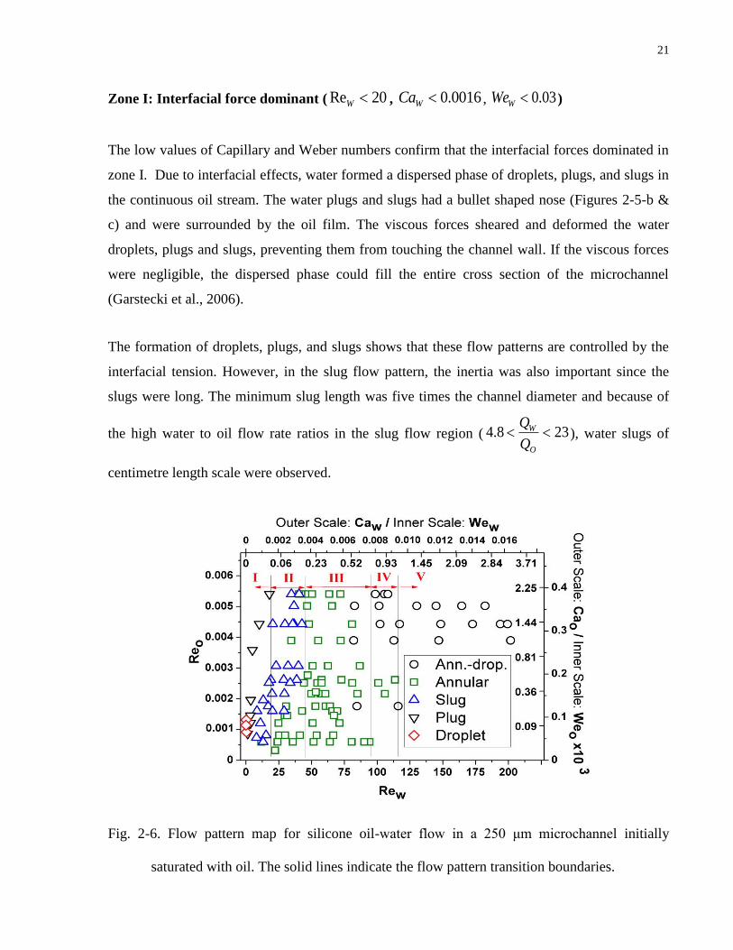
21

Zone I: Interfacial force dominant ( 20Re W , 0016.0WCa , 03.0WWe )

The low values of Capillary and Weber numbers confirm that the interfacial forces dominated in

zone I. Due to interfacial effects, water formed a dispersed phase of droplets, plugs, and slugs in

the continuous oil stream. The water plugs and slugs had a bullet shaped nose (Figures 2-5-b &

c) and were surrounded by the oil film. The viscous forces sheared and deformed the water

droplets, plugs and slugs, preventing them from touching the channel wall. If the viscous forces

were negligible, the dispersed phase could fill the entire cross section of the microchannel

(Garstecki et al., 2006).

The formation of droplets, plugs, and slugs shows that these flow patterns are controlled by the

interfacial tension. However, in the slug flow pattern, the inertia was also important since the

slugs were long. The minimum slug length was five times the channel diameter and because of

the high water to oil flow rate ratios in the slug flow region ( 238.4 O

W

Q

Q), water slugs of

centimetre length scale were observed.

Fig. 2-6. Flow pattern map for silicone oil-water flow in a 250 μm microchannel initially

saturated with oil. The solid lines indicate the flow pattern transition boundaries.

22

Zone II: Interfacial force Inertia ( 46Re20 W , 0037.00016.0 WCa , and

17.003.0 WWe ):

Both slug and annular flows were observed in this zone. When the inertia controlled the flow

pattern, the core flow was continuous. On the other hand, when the interfacial forces controlled

the flow pattern, the core flow became discontinuous and dispersed. Occurrence of both

continuous and discontinuous water flows in the core indicated that inertial and interfacial forces

were comparable in Zone II. In annular flow, although the water core was continuous, sausage-

shaped deformations of the oil-water interface were seen (Figure 2-5-d). These deformations

were frequently observed in all the annular flows and also in the case of long water slugs. The

sausage-shaped interfacial deformation was caused by an interfacial tension effect in the

injection section when water penetrated through a small channel in the annular gap into the oil

stream (Figure 2-4-c). These deformations were stable and moved with the water core through

the microchannel. In Zones II and III, the low values of 0077.0WCa and 73.0WWe indicate

that the interfacial tension effects were strong enough to disturb the interface at the injection

section and form sausage-shaped deformations.

In the work by Zhao et al. (2006), the interfacial tension was dominant in the limit of 1We and

dispersed flows were observed in this limit. However, in the annular flow in Zones II and III of

this work, the water phase remained continuous due to its high flow rates ( 1658.7 O

W

Q

Q).

Since the water core was surrounded and sheared by the viscous oil, it could not occupy the

entire cross section of the microchannel. With an increase in the water flow rate, the only way

for the water to increase its volume fraction was to elongate in the flow direction and form a

continuous core.

The viscous oil film on the microchannel wall always restricted the water flow. The low values

of 0055.0Re O indicate that the viscous forces were always important in all the five zones. In

the annular flow pattern, inertia tended to make the oil-water interface wavy due to shear

instability, while the viscous effects kept the interface smooth (Figure 2-5-e). The growth of any

perturbations or disturbances at the interface required the motion of the oil in the transverse

23

direction which was resisted by the viscous forces in the oil. Viscous forces also competed with

the interfacial tension to keep the water core stable and continuous. For the water core to pinch

off and break up into droplets, it was necessary for the viscous oil to flow radially towards the

centre of the microchannel, but such radial flows were resisted by the high viscosity of the oil

film.

The transition from the dispersed plug and slug flow patterns to continuous annular flow with an

increase in the Capillary number as shown in Figure 2-6 is consistent with the result of the

stability analysis by Guillot et al. (2007). They showed that an increase in the capillary number

would shift the flow pattern from droplet regime to jet regime.

Zone III: Viscous force > Inertia > Interfacial force ( 95Re46 W ,

0077.00037.0 WCa , and 73.017.0 WWe ):

In this zone, two different flow patterns were observed: annular flow and annular-droplet flow

with a smooth oil-water interface. The annular-droplet flow in Zone III was the annular flow

with addition of fine droplets in the oil film (Figure 2-5-f). The oil-water interface was smooth

but showed sausage-shaped distortions due to interfacial tension effects. The smoothness of the

interface indicated that the viscous forces were still controlling and the inertia was not

sufficiently high to make the interface wavy. In the annular-droplet flow pattern, since the water

flow rate was high, a portion of the water flowed as fine droplets in the oil film.

Zone IV: Inertia Viscous force > Interfacial force ( 116Re95 W , 0094.00077.0 WCa

, 1.173.0 WWe )

In this zone, annular flows and annular-droplet flows with smooth or wavy oil-water interface

were observed. When the interface was smooth, the viscous force could be considered to be

greater than the inertia. With an increase in the water flow rate, the inertia increased. Once the

velocity difference between the oil and water became sufficiently high, inertia dominated the

viscous effects and interfacial waves formed due to shear instability (Figure 2-5-g).

24

Zone V: Inertia dominant ( 116Re W , 0094.0WCa , 1.1WWe )

In this zone, only the annular-droplet flow with a wavy water core was observed. Appearance of

the wavy oil-water interface indicated that the inertia in the water phase was dominant and the

velocity difference between the water core and oil film was sufficiently high so that the interface

became wavy due to shear instability. This flow behaviour is similar to that of a water-glycerol

jet from a 10 mm diameter nozzle injected into an oil at 430Re (Webster et al., 2001), where

the Reynolds number was calculated from the jet exit velocity and the nozzle diameter. The jet

became non axi-symmetric and there was no jet pinch-off at this Re number.

Dessimoz et al. (2008) and Zhao et al. (2006) observed a parallel (stratified) flow pattern in

liquid-liquid flows in microchannels while for the initially oil-saturated microchannel in this

work, parallel flow was not observed. The viscous oil was more wetting compared to water and

formed a stable film around the entire inner wall of the microchannel. The oil film kept the water

flowing along the centre of the microchannel and if the water phase was continuous, annular

flow pattern would form. Also, the oil and water could not form a stratified flow because of a

small difference in the liquid densities and negligible effect of gravity on the flow.

Comparison of the oil displacement by the water in different Zones:

More oil was displaced by the water when the water formed a dispersed phase (unstable system)

compared to when the water core formed a continuous phase (stable system). An unstable water

core broke up into droplets, plugs or slugs. The oil was trapped between the water segments and

displaced with the water flow stream. In other words, more oil was displaced by the water in

Zone I where the flow patterns are controlled by the interfacial tension compared to the oil

displaced by water in Zones III and V.

When the water formed a continuous phase, in annular and annular-droplet flows, more oil was

displaced by a wavy water core (Zone V) compared to a smooth water core (Zone III). When

water was injected into a microchannel filled with oil, the flow of the water core displaced the oil

at the centre of the channel while an oil film was left behind on the channel wall. In annular flow

in the microchannel, the only oil displacement mechanism by the water was due to the shear

25

effects at the oil-water interface. The oil film resisted the displacement by water due to its high

viscosity and no slip on the channel wall. When the interface became wavy, the oil was pushed

by the waves and displaced faster with the interfacial wave motions.

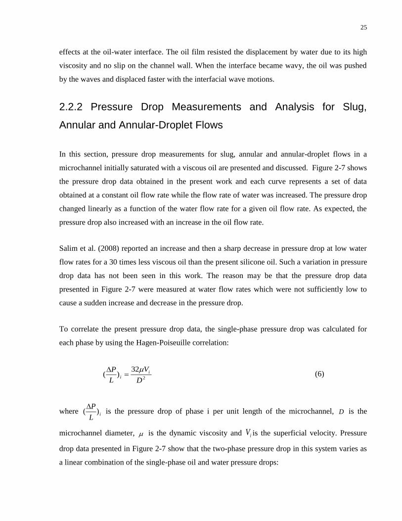
2.2.2 Pressure Drop Measurements and Analysis for Slug,

Annular and Annular-Droplet Flows

In this section, pressure drop measurements for slug, annular and annular-droplet flows in a

microchannel initially saturated with a viscous oil are presented and discussed. Figure 2-7 shows

the pressure drop data obtained in the present work and each curve represents a set of data

obtained at a constant oil flow rate while the flow rate of water was increased. The pressure drop

changed linearly as a function of the water flow rate for a given oil flow rate. As expected, the

pressure drop also increased with an increase in the oil flow rate.

Salim et al. (2008) reported an increase and then a sharp decrease in pressure drop at low water

flow rates for a 30 times less viscous oil than the present silicone oil. Such a variation in pressure

drop data has not been seen in this work. The reason may be that the pressure drop data

presented in Figure 2-7 were measured at water flow rates which were not sufficiently low to

cause a sudden increase and decrease in the pressure drop.

To correlate the present pressure drop data, the single-phase pressure drop was calculated for

each phase by using the Hagen-Poiseuille correlation:

2

32)(

D

V

L

P ii

(6)

where iL

P)(

is the pressure drop of phase i per unit length of the microchannel, D is the

microchannel diameter, is the dynamic viscosity and iV is the superficial velocity. Pressure

drop data presented in Figure 2-7 show that the two-phase pressure drop in this system varies as

a linear combination of the single-phase oil and water pressure drops:

26

OWTPL

PC

L

PC

L

P)()()( 21

(7)

where 1C and

2C are constants, TPL

P)(

is the two-phase pressure drop and W

L

P)(

and O

L

P)(

are the water and oil single-phase pressure drops calculated by using Eq. 6 and superficial

velocities of water and oil, respectively. By using Eq. 6, Equation 7 can be re-written as,

OWTP VCVCL

P43)(

(8)

where 3C and 4C are constants, and WV and OV are the superficial water and oil velocities. The

constants 41 CC that best fit the present oil-water pressure drop data are given in Table 2-1. As

shown in Figure 2-7, Eq. 8 can predict the pressure drop data for this system with a maximum

error of %10 .

It is noted that Eqs. 7 and 8 should be used only when the flow pattern is slug, annular or

annular-droplet flow, and is not valid when the flow pattern is droplet or plug flow. Any pressure

drop correlation for plug and droplet flows should reduce to that for a single-phase flow when

the flow rate of the dispersed phase approaches zero. Equations 7 and 8 do not satisfy this

limiting condition. In the range of flow rates tested in this work, mainly slug, annular and

annular-droplet flows were observed and no pressure drop correlation is proposed for droplet and

plug flow patterns.

The experimental data from Salim et al. (2008) were also used to validate the model proposed in

this study. Equation 8 is correlated with their experimental results for slug and annular flows in

microchannels initially filled with oil. However, Salim et al. (2008) only reported slug flow

pattern for their system and did not differentiate between plug and slug flows. They obtained and

reported pressure drop data for oil-water flows in glass and quartz microchannels with hydraulic

diameters of 667 and 793 μm, respectively. The viscosity and density of the oil used in their

study were 30.6 mPa.s and 843 kg/m3, respectively, and the oil-water interfacial tension was 30.1

mN/m. For their data, different values of the constants 41 CC were obtained for the glass and

27

quartz microchannels as given in Table 2-1. As shown in Figures 2-8 and 2-9, the empirical

pressure drop correlation given by Eq. 8 is also in good agreement with the experimental results

of Salim et al. (2008). The constants 3C and 4C in Eq. 8 are inversely proportional to the channel

diameter squared. The diameter of the microchannel used in this work was about 1/3 of those

used by Salim et al. (2008) resulted in higher values of the constants 3C and4C . Also, the

constant 4C is directly proportional to the oil viscosity which was ~30 times higher than that

used by Salim et al. (2008).

In the present experiments, after the microchannel was initially saturated with oil and

water was injected into the channel, a viscous oil film was formed on the channel wall. The core

flow of water surrounded by the oil film was similar to the single phase flow of water in a

smaller diameter channel as the slowly moving viscous oil film effectively acted as a channel

wall. In the slug, annular and annular-droplet flows in this work, the velocity ratio of water to oil

was high ( 1658.4 O

W

Q

Q), and the oil phase could be considered as a stationary film. Under

these conditions the pressure drop changed linearly with the water velocity which is expected in

a single-phase laminar flow.

For a microchannel initially saturated with oil, Salim et al. (2008) used the Lockhart-Martinelli

correlation to predict the pressure drop which will be discussed later. For an initially water

saturated microchannel, they proposed a linear equation for the two-phase pressure drop

containing separate terms for individual pressure drops in each phase:

OoWTPL

P

L

P

L

P)()()(

(9)

Here, o is the ratio of the volumetric oil flow rate to the total oil-water flow rate and the

parameter depends on the microchannel property. Equation 9 is similar in form to our pressure

drop correlation given by Eq. 7, however, they cannot be directly compared since one of the

coefficients in Eq. 9 includes the oil and water flow rate ratio while the coefficients in Eq. 7 are

constant.

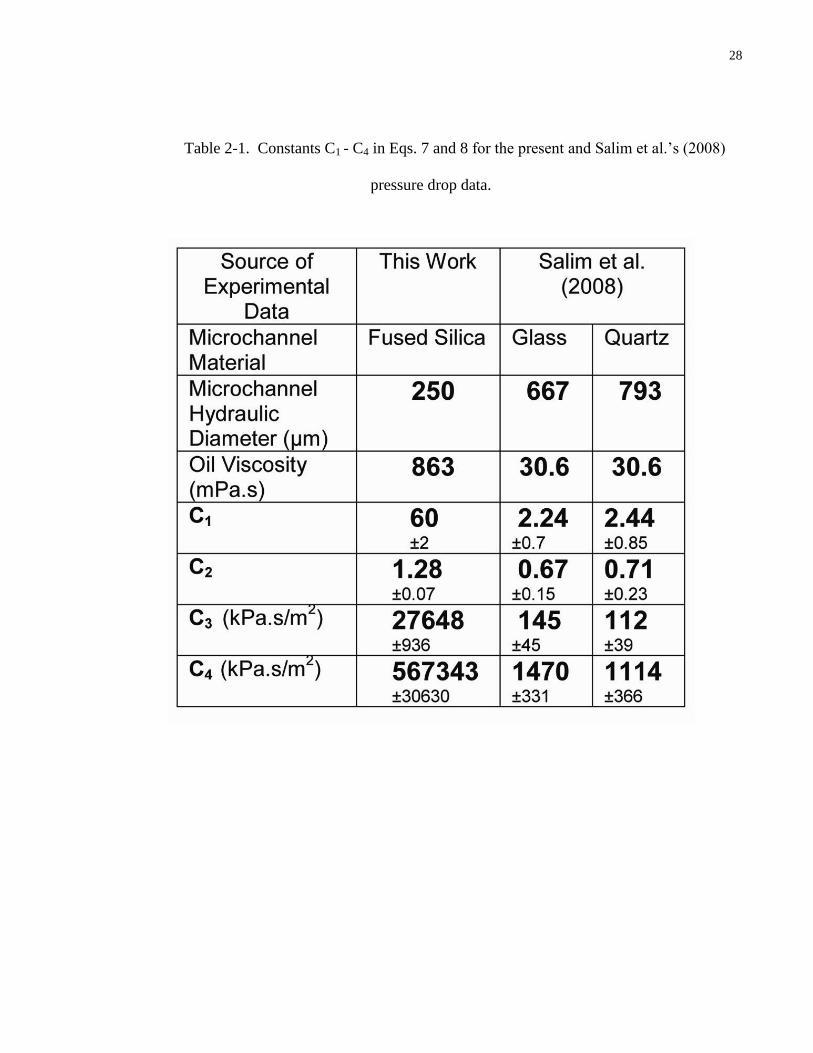
28

Table 2-1. Constants C1 - C4 in Eqs. 7 and 8 for the present and Salim et al.’s (2008)

pressure drop data.

29

Fig. 2-7. Pressure drop data for silicone oil-water flow in a microchannel. The constants in Eq. 8

are 276483 C and 5673434 C .

30

Fig. 2-8. Prediction of Salim et al. (2008)’s pressure drop data for a glass microchannel by Eq. 8

with 1453 C and 14704 C .

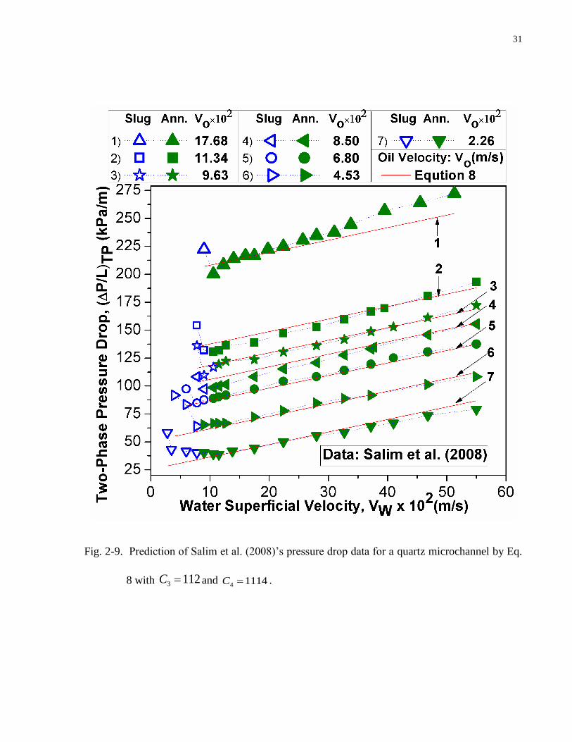
31

Fig. 2-9. Prediction of Salim et al. (2008)’s pressure drop data for a quartz microchannel by Eq.

8 with 1123 C and 11144 C .

32

In the works by Kashid and Agar (2007) and Jovanovic et al. (2011), the liquid-liquid slug flow

pressure drop models included separate terms for the interfacial pressure drop and hydrodynamic

pressure drop, whereas in this work, the effect of interfacial tension is not considered. The

interfacial pressure drop accounts for the pressure drop in the flow direction due to the curvature

of the oil-water interface. In the interfacial force dominant region, water droplets, plugs and

slugs could be formed. Equations 7 and 8 cannot be used for droplet and plug flows. Also,

because of the high water flow rate in the slug flow region ( 238.4 O

W

Q

Q), water slugs in the

present work were long and the two phase pressure drop was due primarily to the contribution of

hydrodynamic pressure drop. However, when Equation 8 was used to predict the experimental

results of Salim et al. (2008), the maximum error occurred in the limit of low water velocity in

the slug flow regime (Figures 2-8 & 2-9). The error might be due to a sharp increase and then a

decrease in the pressure drop in the limit of low water flow rates in their work or the fact that the

interfacial pressure drop effects are ignored in Equation 8.

The pressure drop models presented by Kashid and Agar (2007) and Jovanovic et al. (2011) for

slug flows are more elaborate than the simple model of Eq. 8. Also, the model of Salim et al.

(2008) (Equation 9) includes a flow rate ratio and is more complete than Eq. 8. However, the

advantage of using Eq. 8 is its simplicity. Results presented in Figures 2-7, 2-9 and 2-9 show that

Eq. 8 can be used to predict the pressure drop in an initially oil-saturated microchannel

specifically when both liquids form continuous phases.

Next, a Lockhart-Martinelli correlation was examined to see if it can also be used to

describe the present oil-water two-phase pressure drop data. The two-phase friction multipliers

and the Lockhart-Martinelli parameter are defined as:

W

TPW

LP

LP

)/(

)/(

(10)

O

TPO

LP

LP

)/(

)/(

(11)

33

W

O

O

W

LP

LP

)/(

)/(

(12)

where W is the water-phase friction multiplier, O is the oil-phase friction multiplier and is

the Lockhart-Martinelli parameter. By using Eqs. 7 and 12, Equations 10 and 11 can be written

as:

2

21

2 CCW (13)

22

12C

CO

(14)

Equation 13 is comparable with the Lockhart-Martinelli model that Salim et al. (2008) proposed

for slug and annular flows:

221 W

(15)

where and are constants. Comparing Eqs. 13 and 15, the constant is zero in Eq. 13. When

is zero, the two-phase pressure drop can be calculated from the individual pressure drop in

each phase.

The water-phase friction multiplier, W , the oil-phase friction multiplier, O , and the square of

the Lockhart-Martinelli parameter, 2 , were calculated from the present experimental data. In

Figure 2-10, 2

W is plotted against 2 , while

2

O is plotted against 2

1

in Figure 2-11 along

with Eqs. 13 and 14. Equation 13 shows that 2

W changes linearly with 2 and Eq. 14 shows

that 2

O is proportional to 2

1

. Figures 2-10 and 2-11 show excellent agreement between both

Eqs. 13 and 14 with the present viscous oil-water pressure drop data in a 250 µm diameter

microchannel.

34

Fig. 2-10. Linear variation of the water two-phase friction multiplier,2

W , with Lockhart-

Martinelli parameter, 2 .

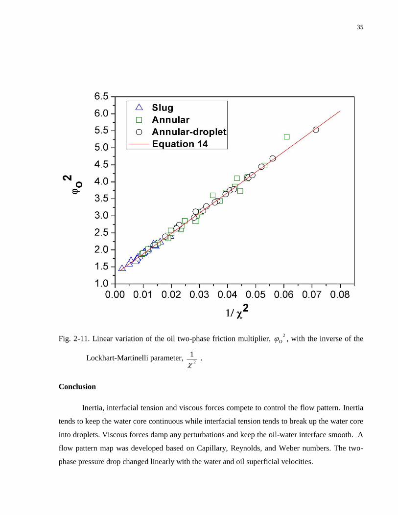
35

Fig. 2-11. Linear variation of the oil two-phase friction multiplier, 2

O , with the inverse of the

Lockhart-Martinelli parameter, 2

1

.

Conclusion

Inertia, interfacial tension and viscous forces compete to control the flow pattern. Inertia

tends to keep the water core continuous while interfacial tension tends to break up the water core

into droplets. Viscous forces damp any perturbations and keep the oil-water interface smooth. A

flow pattern map was developed based on Capillary, Reynolds, and Weber numbers. The two-

phase pressure drop changed linearly with the water and oil superficial velocities.

36

Chapter 3

Immiscible displacement of oil by water in a microchannel: asymmetric

flow behaviour and non-linear stability analysis

The immiscible displacement of oil by water in a circular microchannel was investigated. A

fused silica microchannel with an I.D. of 250 µm was initially filled with a viscous silicone oil.

Then, only water was injected into the channel. We describe our flow observations based on the

two dimensional images captured in the middle of the channel. The water finger displaced the

oil, left an oil film on the channel wall. Eventually, the water finger reached the channel exit and

formed a core-annular flow pattern. The water flow rate and inertia increased with the change in

flow regime to core–annular flow since the flow resistance decreased. The wavelength of waves

formed at the oil-water interface also increased with the increase in inertia. The initially

symmetric interfacial waves became asymmetric with time. Also, the water core shifted from the

centre of the channel and left a thinner oil film on one side. Under all flow rates tested in this

study, as long as the water was continuously injected, the water core was stable and no break up

into droplets was observed. We also discuss the flow stability based on non-linear and linear

stability analyses performed on the core-annular flow.

3.1. Experimental details

3.1.1 Materials

Silicone oil from Sigma Aldrich’s 200 fluid series and De-ionized water were used as the

working fluids. The oil’s surface tension and oil-water interfacial tension were 21 mN/m and

37

43mN/m at 20 °C, respectively. The densities of the two fluids were close ( 1.03water

oil

at 20

°C), while the oil was highly viscous compared to water ( 0.0012water

oil

at 20 °C).

A circular fused silica microchannel (Polymicro Technologies) used in the experiments

was 7.0 cm long and had an inner diameter of 250 μm. Both fluids were wetting and the contact

angles for the oil-channel and water-channel were 25° and 30°, respectively. A schematic

diagram of the apparatus is given in Figure 3-1.

3.1.2 Experimental Facility

The microchannel was first filled with silicone oil and then only water was injected into

the microchannel to displace the oil. As shown in Figure 3-1, a pneumatic pump was used to

inject water into a previously oil-saturated microchannel. The pump consisted of a nitrogen gas

cylinder and a cylindrical stainless steel water reservoir. The reservoir was partially filled with

water and was pressurized at the top by using a compressed nitrogen gas for water injection into

the microchannel. A pressure transducer measured the pressure at the microchannel inlet and the

channel outlet was open to the atmosphere.

A video camera was used to capture images of the water-silicone oil flow. To minimize

the entrance and exit effects on the flow patterns observed, all images were captured in the

middle of the channel at 140 diameters (3.5 cm) downstream of the channel inlet.

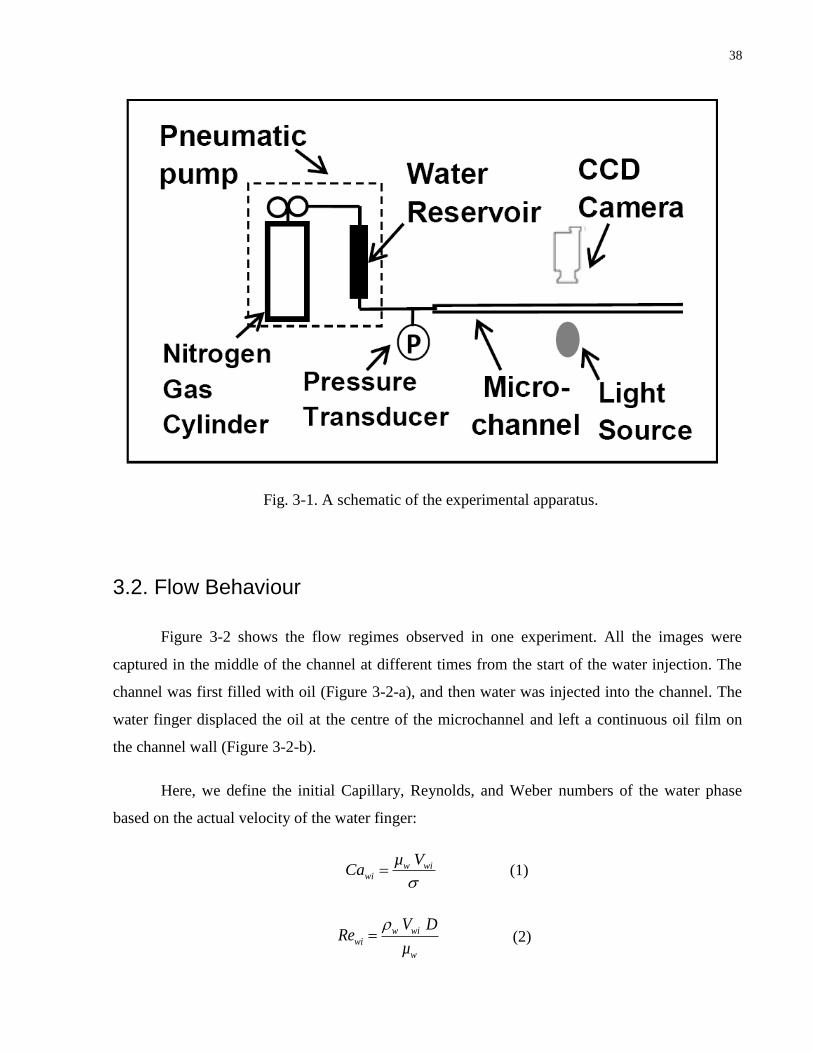
38

Fig. 3-1. A schematic of the experimental apparatus.

3.2. Flow Behaviour

Figure 3-2 shows the flow regimes observed in one experiment. All the images were

captured in the middle of the channel at different times from the start of the water injection. The

channel was first filled with oil (Figure 3-2-a), and then water was injected into the channel. The

water finger displaced the oil at the centre of the microchannel and left a continuous oil film on

the channel wall (Figure 3-2-b).

Here, we define the initial Capillary, Reynolds, and Weber numbers of the water phase

based on the actual velocity of the water finger:

w wiwi

µ VCa

(1)

w wi

wi

w

V DRe

µ

(2)

39

2

w wiwi

V DWe

(3)

where wµ is the viscosity of the water, wiV is the velocity of the finger nose at the centre of

the channel, is the liquid-liquid interfacial tension, w is the density of the water, and D is the

channel diameter. Table 3-1 gives the initial Capillary, Reynolds and Weber numbers of the water

phase for the experiments carried out in this study. The results presented in Figure 3-2 is for

54.8 10wiCa .

Table 3-1. Test conditions.

40

Fig. 3-2. Flow patterns at 5

4.8 10wi

Ca

and 39 10wCa observed in the

middle of the channel (top view) at

different times from the start of the water

injection: a) at t=0 sec, the channel was

filled with oil; b) at t=50.7 sec, the water

finger was displacing the oil at the core;

c) at t=53.3 sec, the oil film was left

evenly on the channel wall and the oil-

water interface was smooth; d-1) at

t=95.5 sec, symmetric perturbations

formed at the interface; d-2) at t=102.5

sec, the wavelength increased; e) at

t=104.2, the water core shifted from the

centre and the flow became asymmetric;

f) at 147.8 sec and g) at t=308.0, the

water core touched one side of the

channel; h) at t=550 sec, the oil was

completely displaced.

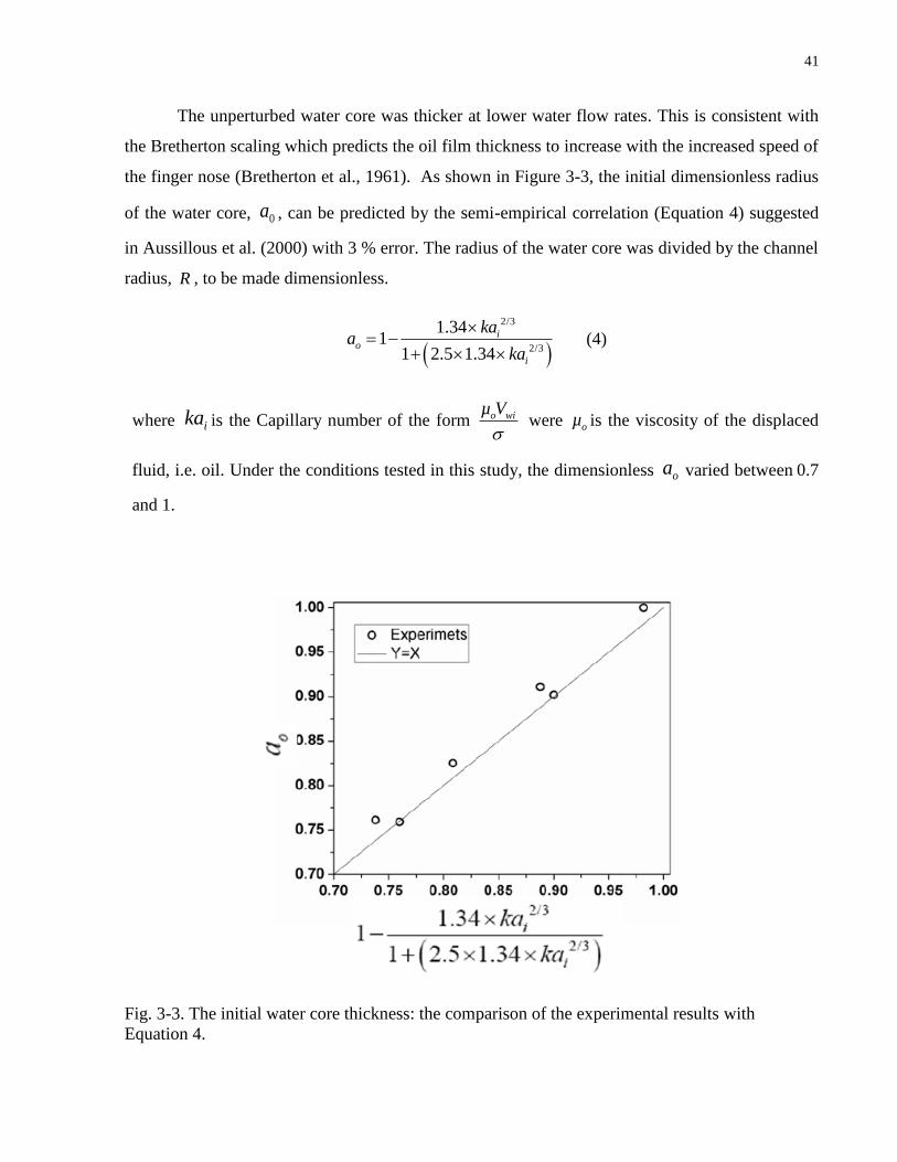
41

The unperturbed water core was thicker at lower water flow rates. This is consistent with

the Bretherton scaling which predicts the oil film thickness to increase with the increased speed of

the finger nose (Bretherton et al., 1961). As shown in Figure 3-3, the initial dimensionless radius

of the water core, 0a , can be predicted by the semi-empirical correlation (Equation 4) suggested

in Aussillous et al. (2000) with 3 % error. The radius of the water core was divided by the channel

radius, R , to be made dimensionless.

2/3

2/3

1.341

1 2.5 1.34

io

i

kaa

ka

(4)

where ika is the Capillary number of the form o wiµ V

were oµ is the viscosity of the displaced

fluid, i.e. oil. Under the conditions tested in this study, the dimensionless oa varied between 0.7

and 1.

Fig. 3-3. The initial water core thickness: the comparison of the experimental results with

Equation 4.

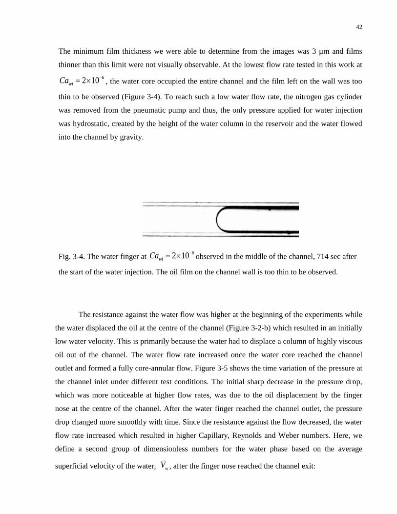
42

The minimum film thickness we were able to determine from the images was 3 µm and films

thinner than this limit were not visually observable. At the lowest flow rate tested in this work at

62 10wiCa , the water core occupied the entire channel and the film left on the wall was too

thin to be observed (Figure 3-4). To reach such a low water flow rate, the nitrogen gas cylinder

was removed from the pneumatic pump and thus, the only pressure applied for water injection

was hydrostatic, created by the height of the water column in the reservoir and the water flowed

into the channel by gravity.

Fig. 3-4. The water finger at 62 10wiCa observed in the middle of the channel, 714 sec after

the start of the water injection. The oil film on the channel wall is too thin to be observed.

The resistance against the water flow was higher at the beginning of the experiments while

the water displaced the oil at the centre of the channel (Figure 3-2-b) which resulted in an initially

low water velocity. This is primarily because the water had to displace a column of highly viscous

oil out of the channel. The water flow rate increased once the water core reached the channel

outlet and formed a fully core-annular flow. Figure 3-5 shows the time variation of the pressure at

the channel inlet under different test conditions. The initial sharp decrease in the pressure drop,

which was more noticeable at higher flow rates, was due to the oil displacement by the finger

nose at the centre of the channel. After the water finger reached the channel outlet, the pressure

drop changed more smoothly with time. Since the resistance against the flow decreased, the water

flow rate increased which resulted in higher Capillary, Reynolds and Weber numbers. Here, we

define a second group of dimensionless numbers for the water phase based on the average

superficial velocity of the water, wV , after the finger nose reached the channel exit:

43

w ww

µ VCa

(5)

Re w ww

w

V D

µ

(6)

2

ww

wVWe

D

(7)

Assuming that the oil velocity is negligible compared to the water velocity, the average

superficial velocity of the water can be calculated by dividing the mixture of the oil and water

flow rate, mQ , by the channel cross sectional area:

21

4

mw

QV

D

(8)

The results presented in Figure 3-2 were at 39 10wCa . As given in Table 3-1, the

values of wCa are two orders of magnitude higher than that of wiCa .

At first, the water core was uniform (Figure 3-2-c), but perturbations started to grow at the

oil-water interface with time and formed travelling waves at the interface (Figure 3-2-d). The time

required for the initiation of perturbations is given in Table 3-1. The initiation and growth of

perturbations took place earlier and faster, respectively, at higher water flow rates. Also, the speed

at which waves travelled along the oil-water interface increased with an increase in the water flow

rate (Table 3-2). The maximum wave speed we were able to measure in our image analyses was

140 mm/s. Also, the maximum wavelength we were able to measure was 5 mm (R

=40). The

wavelengths and wave speeds at 26.7 10wCa and 110wCa were higher than this limit and

are not reported in Table 3-2.

44

Table 3-2. The initial ( a ) and last symmetric ( z ) wavelengths and wave speed. The

experimental values are compared with the results of the non-linear (1f ) and linear (

2f )

analysis.

Fig. 3-5. The variation of the pressure at the channel inlet with time.

45

In each experiment, the interfacial wavelength increased with time. The first wavelength,

a , and also the last symmetric wavelength observed at the interface z , are shown in Figures 3-

2-d-1 and 3-2-d-2. Also, as given in Table 3-2, the ratios of a

z

are less than one which shows that

the wavelength increased with time (compare Figures 3-2-d-1 & 3-2-d-2). The wave speed also

increased with time (Table 3-2). The increase in the wavelength and wave speed could be due to

the increase in the water flow rate after the water finger reached the channel outlet. This

observation is in agreement with the results of the non-linear stability analysis which will be

discussed later. Based on the result of this analysis, the fastest growing wavelength increases with

an increase in inertia (see section 3.3 for the stability analysis).

It should be noted that all descriptions of the flow pattern given are based on the two

dimensional images captured from the system. Although the initiation of disturbances was

symmetrical (Figure 3-2-d), these perturbations did not uniformly grow and the oil-water interface

became asymmetric (Figure 3-2-e). Also, the water core tended to shift towards one side of the

channel and leave a thicker oil film on the other side. At low water flow rates (54.8 10wiCa ),

the water core remained closer to one side (Figure 3-2-f), while at high flow (41.6 10wiCa )

rates, the core position fluctuated between the sides of the channel (Figure 3-6).

It is possible that interfacial perturbations may be caused by fluctuations in injection

pressure as shown by Torralba et al. (2008). However, the pressures of the pneumatic pumps in

this study were regulated and kept constant by a double-stage gas regulator which was connected

to a high pressure nitrogen gas cylinder. In these experiments, the oil-water interface was initially

smooth and perturbations were formed at the interface with time. If the pneumatic pump was

responsible for the interfacial instability, perturbations could be formed at any time and the

interface might not be initially smooth. Compared to other injection methods, pneumatic pumps

can supply fluids at a constant injection pressure. For example, in syringe pumps, the injection

pressure keeps changing while the flow rate is constant.

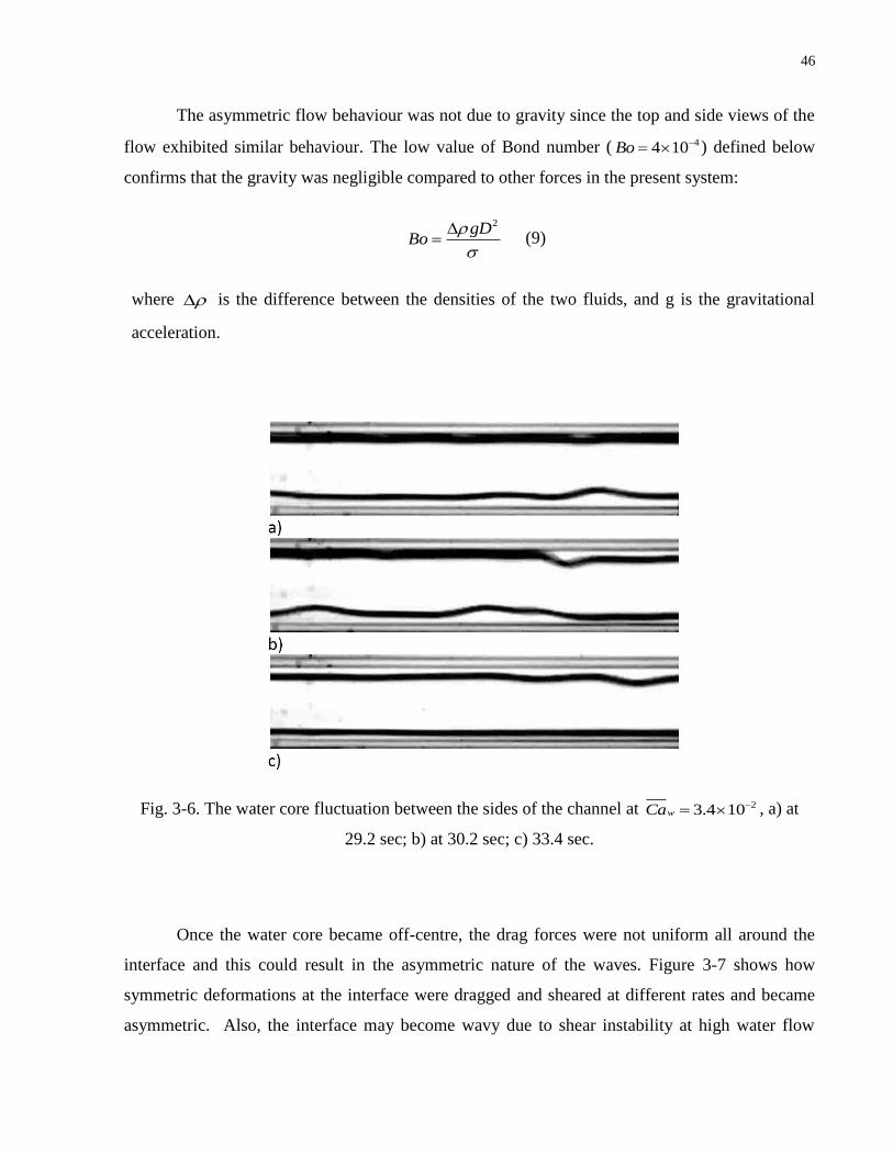
46

The asymmetric flow behaviour was not due to gravity since the top and side views of the

flow exhibited similar behaviour. The low value of Bond number ( 44 10Bo ) defined below

confirms that the gravity was negligible compared to other forces in the present system:

2gD

Bo

(9)

where is the difference between the densities of the two fluids, and g is the gravitational

acceleration.

Fig. 3-6. The water core fluctuation between the sides of the channel at 23.4 10wCa , a) at

29.2 sec; b) at 30.2 sec; c) 33.4 sec.

Once the water core became off-centre, the drag forces were not uniform all around the

interface and this could result in the asymmetric nature of the waves. Figure 3-7 shows how

symmetric deformations at the interface were dragged and sheared at different rates and became

asymmetric. Also, the interface may become wavy due to shear instability at high water flow

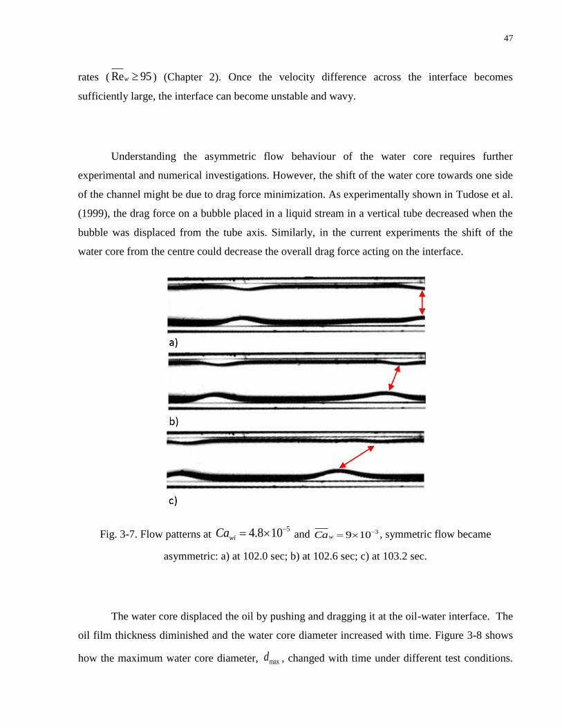
47

rates ( Re 95w ) (Chapter 2). Once the velocity difference across the interface becomes

sufficiently large, the interface can become unstable and wavy.

Understanding the asymmetric flow behaviour of the water core requires further

experimental and numerical investigations. However, the shift of the water core towards one side

of the channel might be due to drag force minimization. As experimentally shown in Tudose et al.

(1999), the drag force on a bubble placed in a liquid stream in a vertical tube decreased when the

bubble was displaced from the tube axis. Similarly, in the current experiments the shift of the

water core from the centre could decrease the overall drag force acting on the interface.

Fig. 3-7. Flow patterns at 54.8 10wiCa and 39 10wCa , symmetric flow became

asymmetric: a) at 102.0 sec; b) at 102.6 sec; c) at 103.2 sec.

The water core displaced the oil by pushing and dragging it at the oil-water interface. The

oil film thickness diminished and the water core diameter increased with time. Figure 3-8 shows

how the maximum water core diameter, maxd , changed with time under different test conditions.

48

At the beginning of the experiments when water was displacing a large oil volume in the core, the

water finger was initially thicker at lower flow rates and the finger nose displaced a larger oil

volume. However, at higher flow rates the water finger displaced less oil volume but at a higher

rate. Also, the drag force at the lateral oil-water interface was higher at higher flow rates and more

oil was dragged at the interface. As shown in Figure 3-8, the complete displacement of the oil

occurred faster at the higher water flow rates.

Fig. 3-8. The variation of the maximum water core radius with time.

To show how the oil film thickness changed with time, the maximum film thicknesses on

both sides ( 1,maxh and 2,maxh where 1,max 2,maxh h ) were measured and the results are presented in

Figure 3-9. Initially, when the water core was at the centre of the channel, 1,maxh and 2,maxh were

equal. The maximum film thickness increased when the perturbations formed at the interface

(compare Figure 3-2-c with 3-2-d). Then 1,maxh and 2,maxh decreased while the oil was being

dragged and pushed out by the water. Once the water core was shifted from the centre, it left a

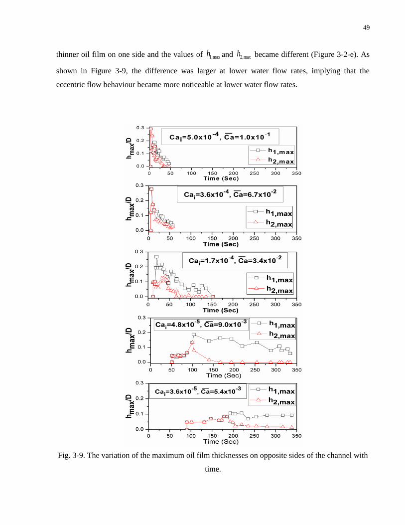
49

thinner oil film on one side and the values of 1,maxh and 2,maxh became different (Figure 3-2-e). As

shown in Figure 3-9, the difference was larger at lower water flow rates, implying that the

eccentric flow behaviour became more noticeable at lower water flow rates.

Fig. 3-9. The variation of the maximum oil film thicknesses on opposite sides of the channel with

time.

50

The wave height decreased faster on the thinner oil film (Figure 3-2-e) and the water core

first touched the side of the channel where the film was thinner (Figure 3-2-f). The wave height

on the thicker oil film also decreased with time while the film was dragged (compare Figure 3-2-f

with 3-2-g). Finally, the water completely displaced the oil layer and occupied the entire

microchannel (Figure 3-2-h).

At all the flow rates tested in this study, as long as the water was continuously injected

into the channel, the water core was always stable. No water core break up was observed and the

water always formed a continuous phase. However, in similar experiments carried out in Aul et al.

(1990) at 6 52.9 10 4.1 10wiCa in a microchannel with an I.D. of 54 µm, the water core

break up always took place. Generally, the interfacial forces competed with inertia to make the

water core unstable (Chapter 2). The interfacial tension forces tend to minimize the energy by

breaking the water core into droplets and decreasing the interfacial area between the two fluids.

On the other hand, the inertia tended to keep the water core continuous. At low values of wiCa in

Aul et al. (1999), the interfacial forces were dominant and the water core break up occurred. In

this study, after the water finger reached the channel outlet, the water flow rate and inertia

increased and the capillary number changed from wiCa to wCa . The increase in the inertia was

sufficiently large to keep the water core stable and also made the system asymmetric. This

indicates that inertia can have an important effect on the stability and also morphology of

immiscible displacement (Chevalier et al., 2006; Dias et al., 2011).

Generally, the system may remain stable while the water flow is maintained, but if the flow is

stopped, the water core break up can occur due to a capillary instability. In one experiment, after

the observation of the asymmetric flow behaviour in the system, the water flow was stopped The

symmetric perturbations appeared again and then the water core broke up. The results of this

experiment are shown in Figure 10. This suggests that the asymmetric behaviour is one of the

flow characteristics. The force due to interfacial tension was always present in the system. Once

the water flow was stopped, there was no inertia to resist the interfacial tension and viscous

forces. The symmetric deformations of the oil-water interface caused by thick for the break up of

the core to take place interfacial tension finally broke up the water core into droplets. However,

the surrounding oil film needs to be sufficiently.

51

Fig. 3-10. A stable water core broke up into droplets after the flow was stopped: a) asymmetric

flow at 23.2 10wCa ; b) at 180 sec after the flow was stopped; c) at 740 sec after the flow was

stopped.

3.3. Stability analysis

Here, we perform a non-linear stability analysis on core-annular flow to predict the

wavelength of perturbations formed at the oil-water interface. The derivations of the non-linear

analysis are given in Appendix I in details. Most of the previous analytical studies of core-

annular flow stability analysis were linear (Guillot et al., 2007). In the case of non-linear core-

annular flow stability analysis, the problem is usually solved numerically (Hu and Joseph, 1989)

or by making the formulation weakly non-linear. In the analysis presented in the thesis which is

purely analytical, the non-linear terms in the Navier-Stokes equations are considered. An

averaging technique by integrating the equations across the cross-section of the channel has been

used in this work which makes the analysis very simple. The present analysis deals with average

velocities which are only functions of flow direction and time while the velocity profiles are a

function of radius as well.

52

We use a similar approach as Funada et al. (2002) to make the equations dimensionless.

The following scales were used: channel radius, R, as the characteristic length, *

 o

WR

as

characteristic velocity, *

R

W as characteristic time and

* *2

oP W as characteristic pressure.

Generally, in the notations, we use V as the velocity and U as the dimensionless velocity. Also, V

and U are the average velocities. The dimensionless Navier-Stokes equations for both phases are:

*

 1( ) ( )

Re

w w w ww

U U dP Uml U r

t z dz r r r

(10)

*

 1 1( )

Re

o o o oo

U U dP UU r

t z dz r r r

(11)

where subscripts w and o represent water and oil, respectively, z is the dimensionless coordinate

in the flow direction, U is the dimensionless z-component of velocity, P is the dimensionless

pressure, *Re is the dimensionless Reynolds number of the form

* o

o

W R

µ

,

w

o

l

is the density

ratio and w

o

µm

µ is the viscosity ratio, t is the dimensionless time and r is the dimensionless

radius ( *Re =0.007, 1.03l , 0.0012m in this work).

The notation used in this analysis is for the case where the more viscous fluid is the outer fluid

and the value of m is less than one. In the case that the more viscous fluid is the inner fluid, the

subscripts w and o should be interchanged in Equations 10 and 11. Also, m , l , and *Re should

be replaced with m̂ , l̂ , and *ˆRe where1

m̂m

, 1

l̂l

and

**    

ˆRe w

w

W R

µ

( Funada et al., 2002).

53

The velocity profiles of the two fluids for core-annular flow are

2 2 2

22

( 1            0    

1

)

2

w w

ra mU U r a

m

a

aa

(12)

2

2

1                              1 

11

2

o o

rU U a r

a

(13)

where  wU and  oU are the dimensionless cross section-averaged water and oil velocities,

respectively. a is the dimensionless radius of the water core, which could be a function of time.

At the interface, the oil and water velocities are equal, i.e. w oU U at r a . Since Equations 12

and 13 satisfy this condition, one can find the relation between the averaged oil and water

velocities,  wU and  oU .

We substitute Equations 12 and 13 into Equations 10 and 11 and then integrate Equation

10 with respect to r dr from 0r to r a and integrate Equation 11 with respect to r dr from

r a to 1r . Integrating the equations allows us to work with average velocities instead of

velocity profiles (Johnson et al., 1991). The integrated Navier-Stokes equations are:

2 2 2 2

2*2

2  1 2( ) ( )

2 2 2 2 Re(1 )

2

ww w w

dPa a a m al U l U U

at z dzm a

(14)

2 2 2

*

21 1 1 1 4( )

2 2 2 2 Re

oo o o

dPa a aU U U

t z dz

(15)

The mass conservation equations for the two fluids are

54

2 2( ) ( )w

d dU a a

dz dt (16)

2 2(1 ) ( )o

d dU a a

dz dt (17)

Following Johnson et al. (1991), we use the perturbations of the form

[1 exp ]oa t ikza (18)

w  υ expwU t ikz (19)

o  υ expoU t ikz (20)

where oa is the radius of the unperturbed water core, is the dimensionless growth rate, 2

k

is the dimensionless wave number and is the dimensionless wavelength. The primes denote the

perturbations. wυ and oυ can be found in terms of , oa and by inserting Equations 18-20

into Equations 16 and 17.

Also, the dimensionless normal stresses must balance at the interface:

2

* 2 2

  1( ) ( )

 w o

o

Pz We z

a a

z aP

(21)

where *We is the Weber number of the form

2*

oW R

and is equal to 1. Equation 21

couples Equations 14 and 15 since it gives the relation between the perturbations in pressures of

the two fluids. After introducing the perturbations into Equations 14, 15, and 21, Equations 14

55

and 15 can be combined into a single equation by using Equation 21. Ignoring all the imaginary

terms, this single equation results in the following dispersion equation for the growth rate:

2

1 0A B C (22)

where the constants A, B, and C1 are

2

22

1

o

o

aA l

a

(23)

2

2* 222 )

28

Re 1 (12

o

ooo

a mB

aa m a

(24)

2

* *

4 2 2

2

2

1

1( )

1

o ow o

o o

a aC k l U U k

aWe We a

(25)

or

2

* 2

4 2

1

1 1 1)

2( )

)2 (1

oo w o

o o

aC a k We We

Wk

a ae

(26)

Where * 1We and ww

w

V DWe

and

ooo

V DWe

are the Weber numbers

calculated by the water and oil properties. wV and oV are the water and oil average velocities,

respectively.

Between the two roots of Equation 22, we choose the one which gives the asymptotic

solution where goes to zero when k goes to zero. The solution to Equation 22 is

56

2 1( )2 2

CB B

A A A (27)

The critical wavelength, 1c , at which the growth rate is zero and the fastest growing

wavelength, 1f , at which the growth rate is maximum can be given by Equations 28 and 29:

2

2

1

1

1

2

(2

 

)1

c o

o o

o

w o

aa a

aWe We

(28)

2

2

1

1

1 ( )2 1

2 2  

w o

f o

o o

o

aa a

e ea

W W

(29)

In the limit of low Re number, the Stokes approximation can be used to describe the system

(Currie, 2003; Guillot et al., 2007). In Stokes equations the inertia terms, i.e. the second terms in

Equations 10 and 11, are neglected and the analysis becomes linear. If one redo the analysis

using Stokes equations the following dispersion equation can be found for the core-annular flow:

2

2 0A B C (30)

where the constant C2 is

4 2

2 *

1(

1)o

o

C a k kWe a

(31)

57

From Equation 30, the following critical and also the fastest growing wavelength can be found in

the limit of low Re number where inertia is negligible:

2 2  c oa (32)

2 2 2  f oa (33)

The results of the linear analysis given by Equations 32 and 33 are in agreement with the results

of the classical theory of the capillary instability of a cylindrical interface (Lord Rayleigh, 1878).

This critical wavelength is also the same as the one given in the analysis of viscous potential

flow presented in Funada et al. (2002). Also, these results are in agreement with the results of

previous analyses of core-annular flows in channels (Hu et al., 1989). In Aul et al. (1990), for the

system of thin film, it was shown that the fastest growing wavelength would be different from

Equation 33 by a factor of 1

1 VC, where VC is the ratio of van der Waals forces to

interfacial tension forces. Also, as experimentally shown in Duclaux et al. (2006), when the

effect of gravity becomes considerable, the fastest growing wavelength would be different from

Equation 32 by a factor of 2

1

1 2.5Bo.

Here we compare the results of the non-linear analysis which considers the effect of inertia with

those of the linear analysis in which the effect of inertia is neglected. In the linear analysis, the

growth rate is a function of the unperturbed water core radius, Re number ( *Re ), the density and

viscosity ratios, and the wave number (Equation 30). In the non-linear analysis, the growth rate is

a function of all these parameters as well as the oil and water Weber numbers (Equation 22).

Figure 3-11 compares the stability of a system predicted by the two analyses. The growth rate

predicted by the linear analysis, in which the effect of inertia is neglected, is unstable over a

58

wider range of wave numbers. Also, for a given unstable wavelength, the growth rate of the

linear analysis is higher than that of the non-linear analysis. This indicates that considering the

inertia effects makes the system more stable which is in agreement with the experimental results.

Generally, inertia tends to keep the water core continuous (Chapter 2). As mentioned earlier,

under the experimental conditions tested in this study, as long as the water was injected into the

channel, inertia kept the water core stable. The water core break up only took place when the

flow was stopped.

Fig. 3-11. Dimensionless growth rate, , vs. dimensionless wave number,2

k

, at

1.03, 0.8, 0.0012,ol a m *Re 0.007 , 0.8wWe and 53 10oWe : the system predicted

by the non-linear analysis is more stable compared to the one predicted by the linear analysis.

59

Based on the results of the linear analysis (Equations 32 and 33), the critical and the fastest

growing wavelengths are only a function of water core radius while in the non-linear analysis

(Equations 28 and 29), these wavelengths are a function of the oil and water Weber numbers as

well. The wavelengths predicted by the non-linear analysis have higher values by a factor of

2

2

1

1 ( )2 1

oo o

w

o

We Wa

ea

a

compared to the values given by the linear analysis. This is in

qualitative agreement with the experimental results where the interfacial wavelengths increased

with an increase in inertia.

A quantitative comparison between the results of Equations 29 and 33 is also made.

Recalling that the relation between the average oil and water velocities is given by Equations 12

and 13 at the interface, two sets of Weber numbers for the oil and water phases were calculated

for each experiments: the initial Weber numbers based on the velocity of the water finger at the

centre of the channel and also the Weber numbers based on the average water and oil velocities

after the water finger reached the channel exit. For the experimental conditions tested in this

study, the factor of 2

2

1

1 ( )2 1

oo o

w

o

We Wa

ea

a

in Equation 29 calculated based on the initial

values of the Weber numbers was very close to unity with a difference less than 0.001. In other

words, both analyses predict the same results in the limit of low initial Weber numbers. Also, in

Figure 3-12-a, the results of the linear and non-linear for the system of oil and water used in this

study are compared with the last symmetric wavelengths observed in the experiments. As shown

in Figure 3-12-a, the results of both analyses give the same values of wavelengths in the limit of

low Reynolds numbers ( 60 Rew ). This suggests that ignoring the inertia terms is a valid

assumption for systems with low Reynolds and Weber numbers. However, as given in Table 3-2,

the results of the two analyses are different when the wavelength in Equation 29 is calculated by

the Weber numbers based on the water and oil velocities after the water finger reached the

channel exit. In the case of linear analysis, the ratio of the last symmetric wavelengths in

experiments to the one given by the analysis, i.e. 2

z

f

, is more than one which indicates that the

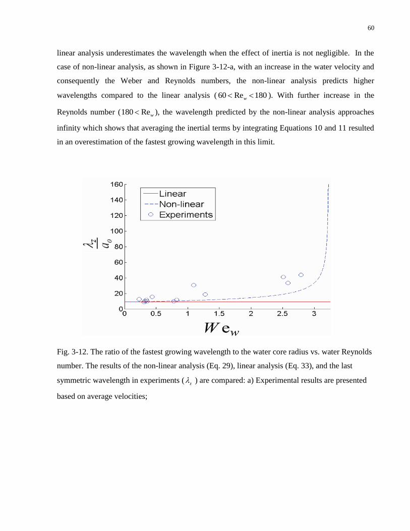
60

linear analysis underestimates the wavelength when the effect of inertia is not negligible. In the

case of non-linear analysis, as shown in Figure 3-12-a, with an increase in the water velocity and

consequently the Weber and Reynolds numbers, the non-linear analysis predicts higher

wavelengths compared to the linear analysis ( 60 Re 180w ). With further increase in the

Reynolds number (180 Rew ), the wavelength predicted by the non-linear analysis approaches

infinity which shows that averaging the inertial terms by integrating Equations 10 and 11 resulted

in an overestimation of the fastest growing wavelength in this limit.

Fig. 3-12. The ratio of the fastest growing wavelength to the water core radius vs. water Reynolds

number. The results of the non-linear analysis (Eq. 29), linear analysis (Eq. 33), and the last

symmetric wavelength in experiments ( z ) are compared: a) Experimental results are presented

based on average velocities;

61

Conclusion

In the immiscible displacement experiments, interfacial wavelengths were sensitive to

inertia. Inertia made the flow asymmetric and kept the water core continuous. Non-linear and

linear analyses were performed for the system of core-annular flow. Compared to a linear

analysis, a non-linear analysis predicts the stability of the system more accurately.

62

Chapter 4

A Miniature Cell for Gas Solubility Measurements in Oils and

Bitumen

A miniature cell has been designed and constructed to measure gas solubility in crude oils

and bitumen. The cell was made of stainless steel with a total internal volume of 1.835 cc and

only an oil sample of 0.4 cc was required for one set of measurements at different pressures. By

using this small cell, the waiting time for reaching equilibrium was less than 10 minutes. The

technique was validated by measuring CO2 gas solubility in two bitumen samples. The results

were compared and found to be in very good agreement with available data. The apparatus was

also used to study the effect of ashphaltene on CO2 solubility in bitumen. It was shown that

ashphaltene had a negligible effect on CO2 solubility in bitumen.

4.1 Experimental Details

4.1.1 Materials

The CO2 solubility was measured in two bitumen samples obtained from Peace River and

provided by Shell Canada Limited. Research grade CO2 with 99.999% purity was purchased

from Linde. The densities of bitumen samples were measured by using a density meter (Anton

Paar, Model DMA38) at temperatures up to 40 °C as shown in figure 4-1. The density of sample

2 at 60 °C was extrapolated by assuming a linear variation of density with temperature. The

SARA (Saturates, Aromatics, Resins, and Ashphaltene) composition of bitumen samples was

determined by using the thin layer chromatography with flame ionization detection (TLC-FID)

method (Carbognani et al., 2007). The SARA composition of both samples is given in table 4-1.

To make ashphaltene-free samples, ashphaltene was removed from a bitumen sample 1 by

following the method developed by Alboudwarej et al. (2002) and using n-heptane as a solvent.

63

Fig. 4-1. Density of bitumen samples and maltene extracted from sample 1 vs.

temperature.

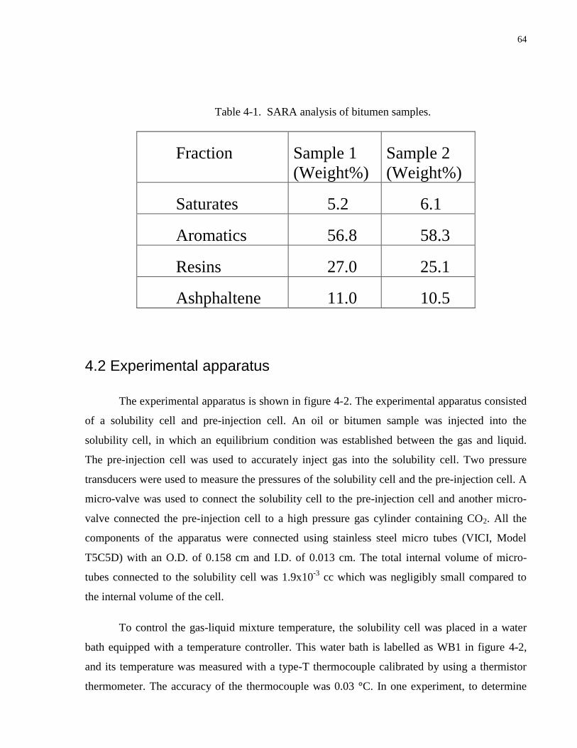
64

Table 4-1. SARA analysis of bitumen samples.

Fraction Sample 1

(Weight%)

Sample 2

(Weight%)

Saturates 5.2 6.1

Aromatics 56.8 58.3

Resins 27.0 25.1

Ashphaltene 11.0 10.5

4.2 Experimental apparatus

The experimental apparatus is shown in figure 4-2. The experimental apparatus consisted

of a solubility cell and pre-injection cell. An oil or bitumen sample was injected into the

solubility cell, in which an equilibrium condition was established between the gas and liquid.

The pre-injection cell was used to accurately inject gas into the solubility cell. Two pressure

transducers were used to measure the pressures of the solubility cell and the pre-injection cell. A

micro-valve was used to connect the solubility cell to the pre-injection cell and another micro-

valve connected the pre-injection cell to a high pressure gas cylinder containing CO2. All the

components of the apparatus were connected using stainless steel micro tubes (VICI, Model

T5C5D) with an O.D. of 0.158 cm and I.D. of 0.013 cm. The total internal volume of micro-

tubes connected to the solubility cell was 1.9x10-3

cc which was negligibly small compared to

the internal volume of the cell.

To control the gas-liquid mixture temperature, the solubility cell was placed in a water

bath equipped with a temperature controller. This water bath is labelled as WB1 in figure 4-2,

and its temperature was measured with a type-T thermocouple calibrated by using a thermistor

thermometer. The accuracy of the thermocouple was 0.03 °C. In one experiment, to determine

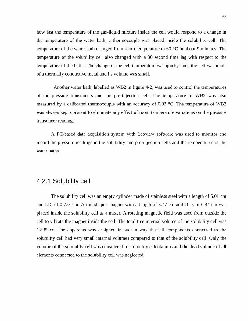
65

how fast the temperature of the gas-liquid mixture inside the cell would respond to a change in

the temperature of the water bath, a thermocouple was placed inside the solubility cell. The

temperature of the water bath changed from room temperature to 60 °C in about 9 minutes. The

temperature of the solubility cell also changed with a 30 second time lag with respect to the

temperature of the bath. The change in the cell temperature was quick, since the cell was made

of a thermally conductive metal and its volume was small.

Another water bath, labelled as WB2 in figure 4-2, was used to control the temperatures

of the pressure transducers and the pre-injection cell. The temperature of WB2 was also

measured by a calibrated thermocouple with an accuracy of 0.03 °C. The temperature of WB2

was always kept constant to eliminate any effect of room temperature variations on the pressure

transducer readings.

A PC-based data acquisition system with Labview software was used to monitor and

record the pressure readings in the solubility and pre-injection cells and the temperatures of the

water baths.

4.2.1 Solubility cell

The solubility cell was an empty cylinder made of stainless steel with a length of 5.01 cm

and I.D. of 0.775 cm. A rod-shaped magnet with a length of 3.47 cm and O.D. of 0.44 cm was

placed inside the solubility cell as a mixer. A rotating magnetic field was used from outside the

cell to vibrate the magnet inside the cell. The total free internal volume of the solubility cell was

1.835 cc. The apparatus was designed in such a way that all components connected to the

solubility cell had very small internal volumes compared to that of the solubility cell. Only the

volume of the solubility cell was considered in solubility calculations and the dead volume of all

elements connected to the solubility cell was neglected.

66

Fig. 4-2. Schematic of the experimental apparatus: 1) water bath 1 (WB1), 2) thermocouple, 3)

solubility cell, 4) magnetic mixer, 5) rotating magnetic field, 6) T-junction, 7) pressure

transducer 1 (P1), 8) micro-valve 1 (V1), 9) pre-injection cell, 10) pressure transducer 2 (P2), 11)

micro-valve 2 (V2), 12) purge valve, 13) gas regulator, 14) CO2 gas cylinder, 15) data

acquisition system, 16) water bath 2 (WB2), 17) computer.

As shown in figure 4-3, two reducing unions (Swagelok, Model SS-600-6-1ZV) with

zero dead volume were used as the cell end fittings to connect the solubility cell to its

neighboring components. These end fittings were compression fittings made of stainless steel,

with which the cell could be easily sealed. The cell alone could withstand a high internal

pressure of up to 42.7 MPa at temperatures below 93°C and 32.4 MPa at temperatures below 537

°C. Also, with these compression fittings, the cell could be readily detached from the apparatus

for cleaning. A plug was used to close one end of the solubility cell while the other side was

connected to a T-junction (Swagelok, Model SS-1F0-3GC), which had a negligible dead volume

67

of 2.8x10-4

cc compared to the volume of the solubility cell. The T-junction connected the

solubility cell to a pressure transducer (Omega, Model PX 5500) and micro-valve (VICI, Model

SFVO) which are labelled as P1 and V1, respectively, in figure 4-2. The accuracy of the pressure

transducer was 7 kPa and it could operate at pressures up to 6.89 MPa. To reduce the internal

dead volume of the pressure transducer to zero, the pressure transducer was first vacuumed and

then filled with mercury. The micro-valve, V1, had an internal volume of 2x10-3

cc which was

again negligibly small compared to the internal volume of the solubility cell.

4.2.2. Pre-injection Cell

To accurately control the amount of gas injected into the solubility cell, the gas was first

injected into the pre-injection cell and then into the solubility cell. The pre-injection cell was an

empty cylinder made of stainless steel. From one end, the pre-injection cell was connected to the

solubility cell via a micro-valve, V1. From the other end, the pre-injection cell was connected to

another pressure transducer (P2) and micro-valve (V2) by using exactly the same type of end

fittings, T-junction and micro tubes used for the solubility cell. The total internal volume of the

pre-injection cell and pressure transducer (P2) was 7.215 cc. V2 and P2 were the same models as

V1 and P1. V2 connected the pre-injection cell to a purge valve and a high pressure gas cylinder.

Fig. 4-3. Schematic of the solubility cell: 1) plug, 2) compression fitting, 3) column end fitting,

4) magnetic mixer, 5) equilibrium cell, 6) micro-tube, 7) T-junction, 8) micro-tube connected to

pressure transducer 1 (P1), 9) micro-tube connected to micro-valve 1 (V1).

68

4.3. Experimental Procedure

The solubility of CO2 was measured in two bitumen samples from Peace River at 22, 35, and 60

°C for the first sample and at 22 and 35 °C for the second sample. Six steps were followed to

measure solubility values as summarized in figure 4-4.

4.3.1 Step 1: Liquid Injection into the Solubility Cell

Liquid samples were injected into the solubility cell before the cell was placed in the water bath,

WB1. First, a plug from one end of the solubility cell was removed. To remove air from the cell,

both micro-valves, V1 and V2, were opened and the cell was purged with CO2 at a pressure

slightly higher than atmospheric pressure. Although the CO2 gas in the cell at the purge pressure

contacted the bitumen sample, the contact time was short and the solubility of CO2 in the sample

at this low pressure was neglected. The vacuum was not applied since light hydrocarbons might

evolve under vacuum and change the liquid sample composition. An oil sample, 0.4 cc in

volume, was manually injected into the cell by using a glass syringe. Liquid samples were

injected uniformly all around the top side of the cell while the cell was kept vertical. The sample

injected slid down and wetted the inner wall of the cell. After the liquid was injected, the cell

was kept horizontally so that the liquid did not accumulate at the bottom of the cell. Figure 4-5

shows how a liquid film was formed inside the cell. Because of gravity, the thickness of the

liquid film on the lower side wall of the cell was thicker than that of the upper part. The

formation of the thin liquid film reduced the waiting time for equilibrium by reducing the

diffusion resistance and providing a very large gas-liquid interfacial area. The plug was replaced

to make the solubility cell closed and sealed. Then the cell was placed in the water bath, WB1,

and its temperature was set to the room temperature.

69

Fig. 4-4. Summary of the experimental procedure for solubility measurements.

70

Fig. 4-5. Formation of a liquid film inside the solubility cell.

4.3.2. Step 2: Gas Injection

4.3.2.1. Step 2-1: Gas Injection into the Pre-injection Cell

The temperature of the water bath, WB2, in which the pressure transducers and pre-injection cell

were placed, was always kept constant at room temperature. For CO2 gas injection, the valve V1

was closed while V2 was left open. The purge valve connected to the gas cylinder was only used

to better adjust the pressure at which the gas was injected into the pre-injection cell when

needed. The gas was first injected into the pre-injection cell from a high pressure gas cylinder

and then V2 was closed. For calculations, the gas density was obtained using a data base from

the National Institute of Standards and Technology (see http://webbook.nist.gov/chemistry for

NIST data base). In this data base, the density of carbon dioxide is calculated by using the

equation of state developed by Span and Wagner (1996). This equation of state considers the

non-ideal behavior of carbon dioxide and is widely used for calculating the properties of carbon

dioxide from its triple point temperature to 1100 K at pressures up to 800 MPa.

To determine the mass of the gas injected into the pre-injection cell, mG,1, the internal volume of

the pre-injection cell, VPre-cell, was multiplied by the gas density, ρG,1, at the pressure and

temperature of the pre-injection cell after the gas was injected into the pre-injection cell.

71

mG,1=VPre-cell × ρG,1 (1)

4.3.2.2. Step 2-2: Gas Injection from Pre-injection Cell into

Solubility Cell

To inject the gas from the pre-injection cell to the solubility cell, V1 was opened and closed.

The amount of gas left in the pre-injection cell, mG,2, was calculated from the CO2 density, ρG,2,

at the pressure and temperature of the pre-injection cell after the gas had been injected into the

solubility cell.

mG,2=VPre-cell × ρG,2 (2)

The difference between the amounts of gas in the pre-injection cell before and after gas injection

into the solubility cell was the amount of gas injected into solubility cell, mG,inj.

mG,inj=mG,1-mG,2 (3)

The measured variables to calculate solubility were temperature and pressure of the pre-injection

and solubility cells. Figure 4-6 shows the changes in the pressure and temperature of the

solubility cell with time.

4.3.3. Step 3: Solubility Measurements at 60 °C

After the gas was injected into the solubility cell, the temperature of the water bath WB1 was set

to 60 °C. As shown in figure 4-6, the pressure in the solubility cell first increased as a result of

an increase in the temperature but after the solubility cell reached 60 °C, the pressure started to

decay as a result of the gas dissolution into the bitumen sample. Finally, the solubility cell

reached a constant pressure indicating the system had reached an equilibrium condition. The

volume of the liquid phase, VL, was determined by dividing the mass of liquid injected into the

solubility cell, mL, by the liquid density, ρL, at equilibrium temperature.

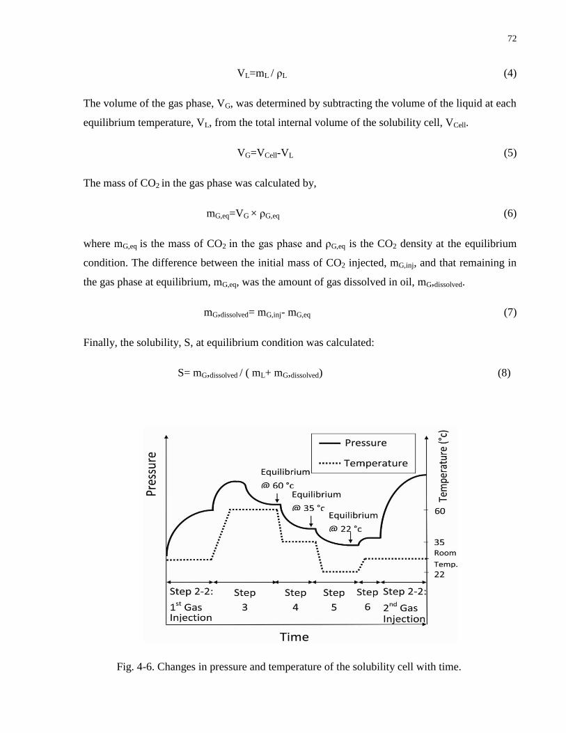
72

VL=mL / ρL (4)

The volume of the gas phase, VG, was determined by subtracting the volume of the liquid at each

equilibrium temperature, VL, from the total internal volume of the solubility cell, VCell.

VG=VCell-VL (5)

The mass of CO2 in the gas phase was calculated by,

mG,eq=VG × ρG,eq (6)

where mG,eq is the mass of CO2 in the gas phase and ρG,eq is the CO2 density at the equilibrium

condition. The difference between the initial mass of CO2 injected, mG,inj, and that remaining in

the gas phase at equilibrium, mG,eq, was the amount of gas dissolved in oil, mG,dissolved.

mG,dissolved= mG,inj- mG,eq (7)

Finally, the solubility, S, at equilibrium condition was calculated:

S= mG,dissolved / ( mL+ mG,dissolved) (8)

Fig. 4-6. Changes in pressure and temperature of the solubility cell with time.

73

4.3.4. Steps 4&5: Solubility Measurements at 35 °C and 22 °C

The same procedure as in step 3 was followed after changing the temperature of the water bath

WB1 and the solubility cell to 35 °C and finally to 22 °C. In this way, the solubility of CO2 gas

in the same bitumen sample was measured at three different temperatures for each gas injection.

4.3.5. Step 6: Changing the Cell Temperature to Room

Temperature for Next Gas Injection

To measure the gas solubility at different pressures and temperatures in the same run, multiple

gas injections were performed. For the second time gas injection, the temperature of the

solubility cell was changed to the room temperature. More gas at a higher pressure than in the

previous gas injection was injected to the solubility cell by following the same gas injection

procedure. The total amount of gas injected into the solubility cell was the sum of the amounts of

gas injected into the cell in current and previous injections. After each additional gas injection,

the temperature of the solubility cell was set to 60 °C again, and then to 35 °C and finally to 22

°C. At each temperature, the solubility was measured at equilibrium. Then the temperature of the

solubility cell was again set to the room temperature and another gas injection was performed.

This procedure was repeated and gas at different pressures was injected into the cell and a wide

range of solubility data at different pressures and three temperatures were collected after

injecting the bitumen sample only once.

After the last solubility measurement, the solubility cell was taken out of the water bath and one

of the end plugs was removed to depressurize the cell. To clean the cell, it was first detached

from the apparatus. Toluene was used as a solvent to wash out the bitumen sample from the cell

and the cell was left in a fume hood for 24 hrs to be completely dry and ready for the next

experiment.

For the bitumen samples studied in this work, a 10 minute waiting time was found to be

sufficient for the system to reach a constant equilibrium pressure. Although the gas-bitumen

mixtures reached equilibrium in less than 10 minutes, the system was left at equilibrium

74

condition for at least one hour to make sure that the pressure did not change with time. This

waiting time for equilibrium is much shorter than that needed for larger cells which may take up

to weeks. However, the new cell used in this work had some minor disadvantages. Although the

cell alone could withstand pressures up to 42.7 MPa, the maximum operating pressure was

limited to the pressure of the gas cylinder used to feed the cell. Since the volume of the cell was

fixed, the gas inside the cell could not be compressed and reach higher pressures above the gas

injection pressure. One other problem was the swelling effect. Oil samples swell as a result of

gas dissolution. Since the solubility cell was opaque, the swelling ratios could not be measured.

4.4. Results and Discussion

The CO2 solubility was measured at 22 and 35 °C for sample 1 and at 22, 35 and 60 °C

for sample 2. Figures 4-7, 4-8 and 4-9 show the CO2 solubility data for the two bitumen samples.

The solubility decreased with an increase in temperature, and increased with increasing pressure.

Both bitumen samples had close solubility values since they were obtained from reservoirs in the

same area and their SARA compositions were quite similar. In figures 4-7 and 4-9, the CO2

solubility data measured in this study are also shown to be in good agreement with the solubility

values for Peace River bitumen reported by Mehrotra and Svrcek (1985b).

The effect of ashphaltene on CO2 solubility was also studied. The ashphaltene-free

bitumen is called maltene and the CO2 solubility in maltene is shown in Figures 4-10, 4-11, and

4-12. As shown in Table 4-1, 11% of the bitumen sample 1 was ashphaltene. To compare the

CO2 solubility in samples with and without ashphatene, the solubility in maltene was

recalculated by including the amount of ashphaltene which was removed from the sample

injected into the cell. Although only maltene was injected into the solubility cell, when equation

8 was used to recalculate the solubility in maltene, the total mass of maltene and removed

ashphaltene was considered as the mass of the liquid phase, mL. As shown in Figures 4-10 & 4-

11, the recalculated solubility values for maltene and the values for bitumen containing

ashphaltene are very close. This confirms that ashphaltene has a negligible effect on CO2

solubility, which is consistent with a very small effect of ashphaltene on the solubility of CO2 in

oil as previously reported by Kokal et al. (1993).

75

For an error analysis, the CO2 solubility results from three runs for sample 1 at 22°C are

compared in Figure 4-12. Since the pressure of the solubility cell decayed as a result of gas

dissolution in bitumen, measurements could not be repeated at exactly the same equilibrium

pressure. But measurements from different runs can be compared by interpolation. By using

interpolation and comparing data from three different runs, the results are found to be

reproducible within 3%.

One source of error in these measurements was the swelling effect. At each equilibrium

condition, the volume of the gas phase was equal to the volume of the equilibrium cell minus the

volume of the liquid. As a result of gas dissolution, the liquid could have swelled and changed its

volume inside the cell resulting in a smaller volume of the gas phase. Since the equilibrium cell

was a blind cell, swelling ratios could not be measured. To analyze the error caused by the

swelling effect, the swelling ratio of sample 1 as a result of CO2 dissolution at 22 °C and at 5.4

MPa was measured by using a glass cell and found to be 1.02. Since the solubility values

reported in this study for sample 1 at 22 °C were measured at equilibrium pressures less than 5.4

MPa, the swelling ratios for all these measurements should be smaller than 1.02. As shown in

Figure 4-13, the solubility values measured at 22 °C in one run were recalculated by assuming a

swelling ratio of 1.02. The recalculated solubility values were higher than the values obtained

without considering the swelling effect with a maximum error of 2.9%.

76

Fig. 4-7. Variation of CO2 gas solubility in bitumen with pressure at 22 °C compared with

solubility data reported by Mehrotra and Svrcek (1985b) for Peace River bitumen.

77

Fig. 4-8. Variation of CO2 gas solubility in bitumen with pressure at 35 °C.

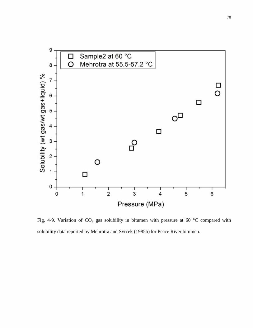
78

Fig. 4-9. Variation of CO2 gas solubility in bitumen with pressure at 60 °C compared with

solubility data reported by Mehrotra and Svrcek (1985b) for Peace River bitumen.

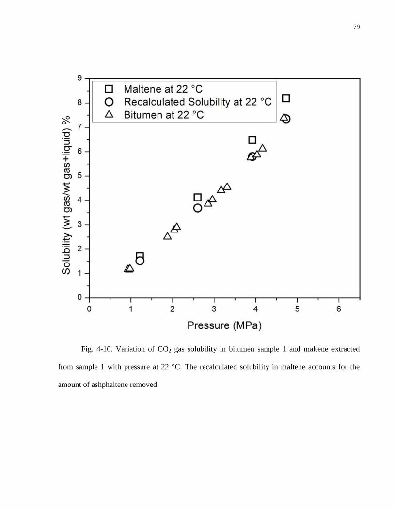
79

Fig. 4-10. Variation of CO2 gas solubility in bitumen sample 1 and maltene extracted

from sample 1 with pressure at 22 °C. The recalculated solubility in maltene accounts for the

amount of ashphaltene removed.

80

Fig. 4-11. Variation of CO2 gas solubility in bitumen sample 1 and maltene extracted

from sample 1 with pressure at 35 °C. The recalculated solubility in maltene accounts for the

amount of ashphaltene removed.

81

Fig. 4-12. CO2 gas solubility data for bitumen sample 1 at 22 °C from three runs.

82

Fig. 4-13. The effect of swelling on CO2 solubility in bitumen sample 1.

4.5 Effect of gas dissolution on flow stability

As a result of the gas dissolution in oil, the oil viscosity would be significantly reduced

and the oil-water viscosity ratio would approach unity. Table 4-2 compares the viscosities of

bitumen and gas saturated bitumen from Peace River measured by Mehrotra et al. (1985b). The

gas dissolution resulted in a significant viscosity reduction. Figure 4-14 shows the effect of

viscosity ratio, w

o

µm

µ , on the linear stability of the system. The maximum growth rate

83

predicted by the linear stability analysis of the core-annular flow (Equation 30 in Chapter 3) vs.

the water to oil viscosity ratio is plotted in this Figure. The maximum growth rate decreases with

an increase in the viscosity ratio which shows that the system becomes more stable with an

increase in the viscosity ratio. Since the gas injection in oil reservoirs results in an increase in the

water to oil viscosity ratio, the gas injection makes the immiscible displacement more stable.

This is in agreement with the result of Guillot et al.’s (2007) analysis, where the flow pattern

may change from droplet regime to jet regime with an increase in m.

Table 4-2. The effect of gas saturation on viscosity of Peace River bitumen

(source: Mehrotra et al., 1985b).

Bitumen CO2 Saturated Bitumen

Temperature (°C)

Pressure

(MPa)

Viscosity

(Pa.s)

Temperature

(°C)

Pressure

(MPa)

Viscosity

(Pa.s)

22 0.1 >23.5 23.8 3.04 6

61.4 0.1 2.37 23.4 4.49 1.86

76 0.1 0.75 22.2 6.1 0.65

85 0.1 0.48 55.5 1.57 1.71

99.5 0.1 0.178 56.2 3 0.84

112.3 0.1 0.102 55.8 4.56 0.47

57.2 6.21 0.3

84

Fig. 4-14. Maximum dimensionless growth rate predicted by linear stability analysis vs.

dimensionless wave number, 2

k

, at 1.03, 0.75,ol a and

*Re 0.007 .

Conclusion

A micro cell with a volume less than 2 ml has been developed for solubility measurements in

bitumen. The available CO2 solubility data in bitumen in literature have been reproduced in much

shorter times, typically less than 9 minutes. Solubility measurements in ashphaltene free bitumen

showed that ashphaltene has little effect on CO2 solubility in bitumen.

85

Chapter 5

Design of a micro glass cell apparatus for pure gas-nonvolatile

liquid phase behavior study

A micro syringe is used as a constant volume cell for gas-liquid equilibrium (GLE) study.

The cell is made of glass and has a volume of less than 100 µl. It can operate at pressures up to

13 MPa and temperatures up to 115 oC. Two different experimental procedures are presented for

systems with non-volatile low and high viscosity liquids. A micro magnetic stir bar is used to

mix the gas-liquid mixtures inside the cell. Since the internal volume of the cell is small, a short

mixing time is sufficient for the gas-liquid mixtures to reach equilibrium. The solubility values

are measured by using the pressure decay method. The experimental procedures are validated by

measuring the carbon dioxide (CO2) solubility in water and highly viscous bitumen. The

experimental results are in good agreement with the available literature data which shows that

the technique works well.

5-1) Experimental details

5-1-1) Materials

Research grade carbon dioxide (CO2) with 99.999% purity was used as the gas phase. Water and

bitumen were used as the low viscosity and highly viscous liquid phases, respectively. To

prepare the water sample, de-ionized water was boiled under vacuum and degassed before it was

injected into the micro cell.

The bitumen sample from Peace River was provided by Shell Canada Limited. The SARA

(Saturates, Aromatics, Resins, and Ashphaltene) composition of the bitumen sample was

determined by using the thin layer chromatography with flame ionization detection (TLC-FID)

method (Carbognani et al., 2007). The bitumen sample contained 5.2 % saturates, 56.8 %

aromatics, 27.0 % resins, and 11.0 % ashphaltene. The density of the bitumen sample was

0.99g/cm3 at 22

oC and its viscosity was 1.6 Pa.sec at 50

oC.

86

5-1-2) Experimental apparatus

The experimental apparatus consisted of three parts: 1) micro cell, 2) gas line, and 3) liquid line.

The schematic of the apparatus is shown in Figure 5-1.

Figure 5-1. Schematic of the experimental apparatus consisting of three parts: the micro cell, gas

line, and liquid line. The schematic is not to scale.

87

5-1-2-1) Micro cell

In this apparatus, a gas-tight glass syringe (Hamilton Syringe, Model 1710) with a volume of 100

µl was used as the micro glass cell (Figure 5-2). The length of the syringe was 6 cm and its bore

size was 1.457 mm. The syringe could operate at temperatures up to 115 °C. For the solubility

measurements in low viscosity liquids, the standard needle of the glass syringe with an inner

diameter of 0.4 mm (Hamilton Removable Needle, Gauge 22) was replaced with a thinner needle

(Hamilton Needle, Gauge 34) which had an inner diameter of 0.05 mm and a length of 38 mm.

The internal volume of this needle was 0.045 µl. The outer diameter of the needle was only 0.16

mm and a 1/16 inch stainless steel tube was used as a support to keep the needle straight. The

needle was inserted into the tube and glued to it.

To prevent leakage at high pressures, the plunger of the syringe was glued to the inner cell wall

using an epoxy glue. After the plunger was glued, the micro cell was tested to be gas tight at

pressures up to 13 MPa. The volume of the cell was constant, since the plunger could not be

moved.

A miniature magnetic stir bar with a volume of 2 µl was placed inside the cell as a mixer. A

magnet placed outside the cell was used to move the stir bar up and down inside the cell. The

free volume of the cell, cellV , was calculated by subtracting the volume of the stir bar, barstirr

V ,

from the volume of the syringe, syringeV .

As shown in Figure 5-1, the temperature of the cell was controlled by a cooling or heating fluid

from a constant temperature bath circulated through a glass jacket placed around the cell. To

thermally isolate the cell, all the components connected to the cell at both ends were insulated.

Two type T thermocouples were used to measure the temperature of the coolant or the heating

fluid at the inlet and outlet of the jacket. These thermocouples had an accuracy of 0.2 ºC and

were calibrated by using a thermistor thermometer. To ensure that the cell temperature could be

precisely controlled by the jacket temperature, the plunger was replaced with a thermocouple in a

set of experiments. In each experiment, the thermocouple was placed at a different height in the

cell and then the cell was sealed. The cell temperature was compared with the temperature of the

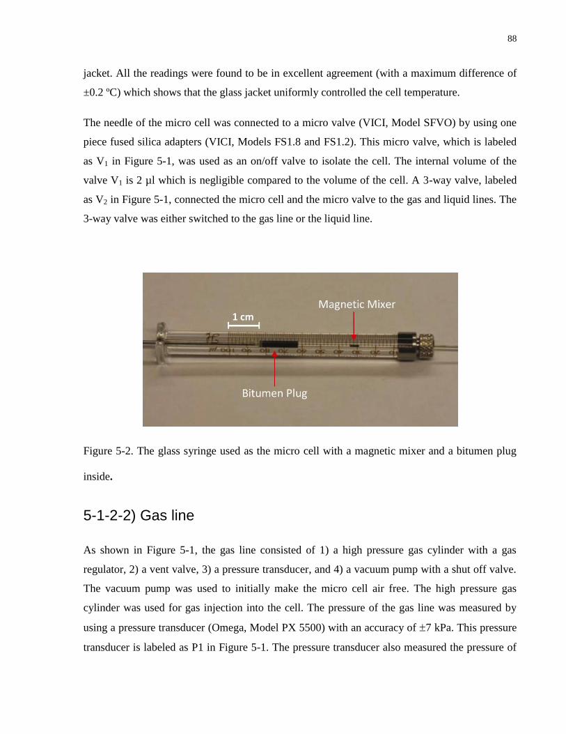
88

jacket. All the readings were found to be in excellent agreement (with a maximum difference of

±0.2 ºC) which shows that the glass jacket uniformly controlled the cell temperature.

The needle of the micro cell was connected to a micro valve (VICI, Model SFVO) by using one

piece fused silica adapters (VICI, Models FS1.8 and FS1.2). This micro valve, which is labeled

as V1 in Figure 5-1, was used as an on/off valve to isolate the cell. The internal volume of the

valve V1 is 2 µl which is negligible compared to the volume of the cell. A 3-way valve, labeled

as V2 in Figure 5-1, connected the micro cell and the micro valve to the gas and liquid lines. The

3-way valve was either switched to the gas line or the liquid line.

Figure 5-2. The glass syringe used as the micro cell with a magnetic mixer and a bitumen plug

inside.

5-1-2-2) Gas line

As shown in Figure 5-1, the gas line consisted of 1) a high pressure gas cylinder with a gas

regulator, 2) a vent valve, 3) a pressure transducer, and 4) a vacuum pump with a shut off valve.

The vacuum pump was used to initially make the micro cell air free. The high pressure gas

cylinder was used for gas injection into the cell. The pressure of the gas line was measured by

using a pressure transducer (Omega, Model PX 5500) with an accuracy of 7 kPa. This pressure

transducer is labeled as P1 in Figure 5-1. The pressure transducer also measured the pressure of

89

the main cell when the cell was connected to the gas line. The vent valve, V5 in Figure 5-1, was

only used to better adjust the pressure of the gas line if it was required.

5-1-2-3) Liquid line

The liquid line is composed of 1) a stainless steel syringe with a manual stage, 2) a liquid

reservoir with an on/off valve and 3) a pressure transducer. The stainless steel syringe (KD

Scientific, Model 78-0801) was used for liquid injection into the micro cell. The plunger of the

stainless steel syringe was supported and moved by the manual stage. The stainless steel syringe

was filled with liquid from the liquid reservoir. The pressure of the liquid line was measured by

the pressure transducer (Omega, Model PX 5500), labeled as P2 in Figure 5-1. This pressure

transducer also measured the pressure of the micro cell when the 3-way valve was switched to

the liquid line.

5-1-3) Experimental procedure for systems with low viscosity

liquids

Five steps were followed to measure the gas solubility (CO2) in the low viscosity liquid (water).

In the first step, the cell was vacuumed. Then, in step 2, the gas was injected into the micro cell

at room temperature. In step 3, liquid was injected into the cell. After the gas and liquid

injections, in step 4, the temperature of the cell was changed from the room temperature to the

temperature at which the solubility was measured. Finally, in step 5, the gas and liquid inside the

cell were mixed and brought to equilibrium and the solubility was measured at the equilibrium

pressure.

5-1-3-1) Vacuuming the cell

In the first step, the micro cell was vacuumed to eliminate air. The lowest pressure that could be

achieved with the vacuum pump was 40 kPa. Since lower pressure was not reachable, the

residual air was diluted with the gas from the high pressure cylinder after the vacuuming, and

then the cell was vacuumed for the second time. This process was repeated at least three times

to make the cell air free.

90

5-1-3-2) Gas injection into the cell

A cooling or heating fluid at room temperature, Troom, was circulated through the jacket

surrounding the micro cell. This way, the temperature of the cell was kept constant at room

temperature for gas injection. The pressure of the gas regulator was adjusted to the pressure,

.inj

gP , at which the gas would be injected into the cell. The micro valve V1 was opened and the 3-

way valve connected the micro cell to the gas line. The valve V3 was also opened and the gas

was injected into the cell (Figure 5-3-a). The pressure transducer P1 measured the pressure of the

gas line and also the micro cell. After the pressure of the cell became stable and equal to .inj

gP ,

the micro valve V1 was closed. The amount of the gas injected into the cell was calculated from,

.. inj

gcell

inj

g Vm (1)

where .inj

gm is the mass of the gas injected into the micro cell, cellV is the volume of the micro

cell, and .inj

g is the density of the gas at room temperature and at the gas injection pressure,

.inj

gP . For calculations, the gas density was obtained from the National Institute of Standards and

Technology (NIST) database (See http://webbook.nist.gov/chemistry for NIST database).

After the gas was injected and V1 was closed, the gas line was vacuumed for the second time

(Figure 5-3-b). This prevented the liquid, which would be injected in the next step, from

introducing additional gas into the cell.

5-1-3-3) Liquid injection into the cell

The 3-way valve was switched to the liquid line. The stainless steel syringe was first filled with

liquid from the liquid reservoir. The pressure transducer P2 indicated the pressure of the liquid

line. The pressure of the micro cell at this point was .inj

gP and the liquid should be injected at a

pressure higher than the cell pressure. Before injecting the liquid into the cell, the pressure of the

liquid line was increased to a pressure, .inj

lP , higher than .inj

gP by pushing the plunger of the

stainless steel syringe forward while the micro valve V1 was closed. After the pressure of the

liquid line was increased, V1 was opened and the liquid was injected into the micro cell (Figure

91

5-4). The injected gas could not escape from the cell while liquid was being injected, since the

pressure of the liquid line was higher than the pressure of the cell. The pressure transducer P2

also measured the pressure of the cell while the 3-way valve was switched to the liquid line and

V1 was opened. Figure 5-5 shows the change in the pressure of the cell in each step.

Figure 5-3. Schematic of the gas line and the micro cell for gas injection process: a) The gas has

been injected into the cell at pressure Pginj.

and at room temperature; b) The valve V1 is closed

and the gas line is vacuumed for the second time before the liquid injection.

92

Since the volume of the cell was constant, the gas volume and pressure inside the cell were

controlled by injecting more sample liquid into the cell. In other words, the liquid sample was

used as a piston to pressurize the gas-liquid mixture inside the cell. By using the stainless steel

syringe for sample liquid injection in the liquid line, it was possible to inject the liquid at a

sufficiently high pressure into the cell.

Figure 5-4. Schematic of the liquid line and the micro cell for liquid injection. The liquid is

injected at pressure Plinj.

which is higher than the pressure of the gas injection.

5-1-3-4) Temperature adjustment

As mentioned earlier, the temperature of the cell was controlled by circulating a constant

temperature coolant or heating fluid through the glass jacket surrounding the cell. After the gas

and the liquid were injected into the cell, the temperature of the cell was changed from the room

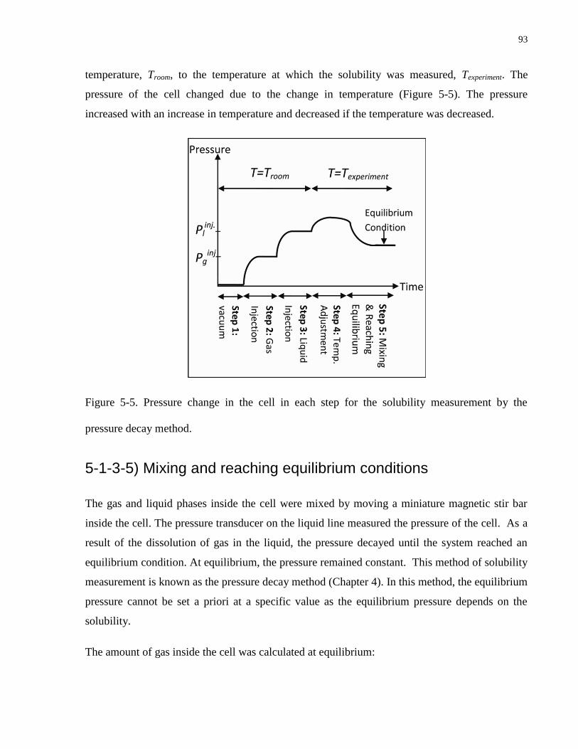
93

temperature, Troom, to the temperature at which the solubility was measured, Texperiment. The

pressure of the cell changed due to the change in temperature (Figure 5-5). The pressure

increased with an increase in temperature and decreased if the temperature was decreased.

Figure 5-5. Pressure change in the cell in each step for the solubility measurement by the

pressure decay method.

5-1-3-5) Mixing and reaching equilibrium conditions

The gas and liquid phases inside the cell were mixed by moving a miniature magnetic stir bar

inside the cell. The pressure transducer on the liquid line measured the pressure of the cell. As a

result of the dissolution of gas in the liquid, the pressure decayed until the system reached an

equilibrium condition. At equilibrium, the pressure remained constant. This method of solubility

measurement is known as the pressure decay method (Chapter 4). In this method, the equilibrium

pressure cannot be set a priori at a specific value as the equilibrium pressure depends on the

solubility.

The amount of gas inside the cell was calculated at equilibrium:

94

... eq

g

eq

g

eq

g Vm (2)

where .eq

gm is the mass of the gas at equilibrium, .eq

gV is the volume of the gas phase at

equilibrium, and .eq

g is the density of the gas at equilibrium condition. In this calculation, it is

assumed that the liquid vapor pressure was negligible compared to the gas pressure and .eq

g was

equal to the pure gas density. Ren et al. (2007) experimentally showed that this assumption is

valid for high pressure gas-liquid systems by comparing their solubility results for decane-CO2

mixtures with the data obtained by using analytical methods. However, this assumption may not

be valid for vapor-liquid equilibrium (VLE) studies and also for systems including highly

volatile liquids. Also, this method cannot be used for gas mixtures since the composition of the

gas at equilibrium is unknown. The error introduced by neglecting the liquid vapor pressure will

be calculated and discussed later.

While the gas was being dissolved in the liquid and the gas-liquid mixture was reaching

equilibrium, the cell was opened to the liquid line. Since the cell was not isolated, the gas could

also diffuse through the needle. The total amount of the gas dissolved in the liquid inside the cell,

dissolved

gm , is given by the difference between the initial amount of the gas injected into the cell,

.inj

gm , and the sum of the amount of the gas at equilibrium, .eq

gm , and the amount of the gas that

diffused through the needle, diffused

gm .

difussed

g

eq

g

inj

g

dissolved

g mmmm ..

(3)

The gas solubility in the liquid sample, W , at the equilibrium pressure and temperature was

calculated by dividing the amount of the gas dissolved in liquid, dissolved

gm , by the sum of the

liquid injected into the cell, lm and dissolved

gm .

dissolved

g

dissolved

l g

mW

m m

(4)

The molar concentration of the gas in the liquid at equilibrium,.eq

gC , can also be calculated by,

95

..

. )/(eq

l

g

dissolved

g

eq

l

dissolved

geq

gV

Mm

V

nC (5)

where dissolved

gn is the number of moles of the gas dissolved in the liquid, .eq

lV is the volume of the

liquid phase at equilibrium and gM is the gas molecular weight.

The amount of the gas diffused through the needle was assumed to be negligible compared to the

amount of the gas dissolved in the liquid inside the cell and was not considered in the solubility

calculations. The error caused by neglecting the gas diffusion through the needle will be

discussed later.

5-1-4) Experimental procedure for systems with highly viscous

liquids

The method presented above may not be applicable to systems comprised of highly viscous

liquids. To minimize the gas diffusion through the needle, a very thin needle with an inner

diameter of 0.05 mm (gauge 34) was used as the cell end connection. It may not be possible to

inject a highly viscous liquid such as bitumen through this needle into the cell at high pressures.

Also, in the solubility measurements in low viscous liquids, the gas diffusion through the needle

is neglected. This error may become considerable for the systems with highly diffusive gases and

also for the systems with highly viscous liquids which require a long mixing time. However, the

experimental procedure can be modified in a way that uses the same experimental apparatus even

for viscous liquids. To validate the modified experimental procedure, the solubility of CO2 in a

bitumen sample from Peace River was measured. For these experiments, a gauge 22 needle with

an inner diameter of 0.4 mm was used as the cell end connection. The cell was mounted

horizontally. Also, the liquid lines in Figure 5-1 were completely filled with mercury instead of

the test liquid. The steps for solubility measurements in the bitumen were as follows:

5-1-4-1) Manual bitumen injection

First, the plunger of the cell (syringe) was removed so one end of the cell was open while the

other end was connected to the gas and the mercury lines. Vacuum could not be applied to make

the cell air free since light components of bitumen might evolve under vacuum and change the

96

bitumen composition. Instead of using vacuum, the cell was purged with gas (CO2) to push the

air out prior to the bitumen injection. Then, a known amount of liquid, lm , was manually

injected from the plunger side into the purged cell. The plunger was then placed inside the cell

and glued to prevent leakage. The plunger pushed the injected bitumen and formed a bitumen

plug inside the cell (Figure 5-6).

Fig. 5-6. The micro cell for CO2 solubility measurements in bitumen: bitumen, CO2, and mercury

are injected into the cell before the start of the mixing.

5-1-4-2) Gas injection

After the bitumen injection, the gas was injected into the cell from the high pressure gas

cylinder. If the gas was suddenly injected into the cell at a high pressure, the gas could finger

into the bitumen plug. To avoid perturbing the bitumen plug, the discharge pressure of the gas

cylinder and consequently the cell pressure were slowly increased until they reached the set

injection pressure. The free volume of the cell for gas injection was equal to the total cell

volume, cellV , minus the injected liquid volume, .inj

lV , so the mass of the gas injected could be

calculated as follows.

. . .( )inj inj inj

g cell l gm V V (6)

97

In this calculation, possible gas dissolution in the liquid during the gas injection process is

ignored. Since the bitumen was first injected prior to the gas injection, some gas might dissolve

into the bitumen during the gas injection. However, the only solubility mechanism in the bitumen

plug during the gas injection was by molecular diffusion. The mixing was always started after

the amount of the injected gas was determined.

5-1-4-3) Mercury injection

The valve V1 was closed and all the steps mentioned earlier for the gas solubility measurements

in water after the gas injection were exactly followed except for the injection of mercury into the

cell instead of water (Figure 5-6). The mercury, which is an inert material, was used as a piston

to control the pressure and also the mixture volume inside the cell. Also, the mercury was used

as a transmitting medium for the pressure transducer, P2.

The mixing process played an important role in bringing the gas-bitumen mixture into

equilibrium inside the cell. Since the bitumen plug, initially formed after the plunger was placed,

resisted the gas dissolution, a magnetic mixer was used to spread the bitumen plug inside the

cell. For the bitumen sample used in this study, a 90 minute mixing time was sufficient for the

system to reach complete equilibrium.

As mentioned earlier, the gas injection method presented here for the systems of viscous liquids

may introduce some errors in calculations. Since the bitumen plug was first injected, the gas

might have dissolved in the liquid during the gas injection process. To accurately calculate the

amount of the gas injected into the cell, in Chapter 4, we used an auxiliary cell (pre-injection

cell) for gas injection. Figure 5-7 shows the schematic of the design presented in Chapter 4. The

pre-injection cell was an empty cylindrical vessel which was directly connected to the main cell.

The gas was first injected into the pre-injection cell. Then, from the pre-injection cell, the gas

was injected into the main cell which contained the bitumen sample. The difference between the

amounts of the gas in the pre-injection cell before and after the gas injection into the main cell

was equal to the amount of the gas injected into the main cell. The experimental results of this

work will be compared with those presented in Chapter 4 later.

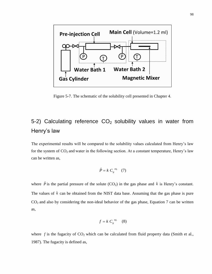
98

Figure 5-7. The schematic of the solubility cell presented in Chapter 4.

5-2) Calculating reference CO2 solubility values in water from

Henry’s law

The experimental results will be compared to the solubility values calculated from Henry’s law

for the system of CO2 and water in the following section. At a constant temperature, Henry’s law

can be written as,

.ˆ eq

gCkP (7)

where P̂ is the partial pressure of the solute (CO2) in the gas phase and k is Henry’s constant.

The values of k can be obtained from the NIST data base. Assuming that the gas phase is pure

CO2 and also by considering the non-ideal behavior of the gas phase, Equation 7 can be written

as,

.eq

gCkf (8)

where f is the fugacity of CO2 which can be calculated from fluid property data (Smith et al.,

1987). The fugacity is defined as,

99

dGRT

fd1

ln (9)

where R is the gas constant, T is the absolute temperature and G is the Gibbs energy. The Gibbs

energy is defined as

TSHG (10)

where H is enthalpy and S is entropy. Substituting Equation 10 into Equation 9 and then

integrating Equation 9 from a low-pressure reference state (indicated by *) to the state of the

experimental condition, yields

*)](*

[1

*ln SS

T

HH

Rf

f

(11)

If the pressure of the reference-state is low enough that the fluid behaves as an ideal gas, then

** Pf in Equation 11, where *P is the pressure of the reference state. In this work, at each

temperature, 1* P kPa was considered as the reference state.

The fluid properties were obtained from the NIST database and fugacity values were calculated

from Equation 11. Then, the values of .eq

gC were calculated from Equation 8 and converted to

W by using Equations 4 and 5 for comparison with the experimental results.

5-3) Experimental results

For the solubility measurements of CO2 in water, after mixing was started in the micro cell, an 8-

minute waiting time was found to be sufficient for the system to reach equilibrium. The

measured solubility of CO2 in water is shown in Figure 5-8 and compared with the data

published in Perry’s Chemical Engineers’ Handbook (Perry et al., 1997). The measurements

could not be repeated at exactly the same equilibrium pressure because the pressure of the cell

decayed as a result of gas dissolution in liquid. However, the experimental results could be

qualitatively compared to those given in Perry’s Handbook since the equilibrium pressures were

close. Also, in Figure 5-8, the experimental results are compared to the values calculated by

100

using Henry’s law. The experimental results are in good agreement with the solubility values

calculated from Henry’s law since the maximum error is 6 %.

Figure 5-9 compares the values of CO2 solubility in the bitumen sample measured with the

present apparatus with the results presented in Chapter 4. The results are in good agreement

which shows the error caused by the CO2 dissolution in the bitumen plug during the gas injection

can be neglected. In the next section, possible sources of error in the solubility measurements

will be discussed.

Figure 5-8. CO2 solubility in water variation with pressure at temperatures of 31, 35, 40, and 50

oC. The solubility values measured in this study are compared with the reference values (Perry et

al., 1997) and the values calculated from Henry’s law (Equation 8).

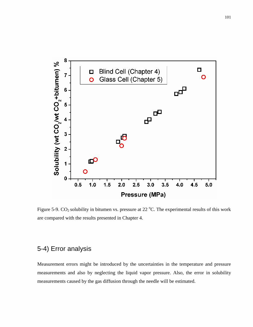
101

Figure 5-9. CO2 solubility in bitumen vs. pressure at 22 oC. The experimental results of this work

are compared with the results presented in Chapter 4.

5-4) Error analysis

Measurement errors might be introduced by the uncertainties in the temperature and pressure

measurements and also by neglecting the liquid vapor pressure. Also, the error in solubility

measurements caused by the gas diffusion through the needle will be estimated.

102

5-4-1) Error due to the uncertainty in temperature and pressure

measurements

The pressure and temperature measurement resolutions in the experiments were 7 kPa and 0.2

°C. For each measured CO2 solubility in water, the maximum and minimum solubility values

were calculated based on a 7 kPa error in pressure measurements, i.e. . 7inj

gP kPa ,and

. 7eqP kPa where .inj

gP and .eqP are the gas injection pressure and the equilibrium pressure,

respectively. In other words, the solubility values were recalculated considering the combination

of the errors in .inj

gP and .eqP measurements. The solubility calculations were also repeated for

each experiment by considering the error in temperature measurements, i.e. 0.2 C uncertainty in

the room temperature at which the gas was injected and 0.2 C uncertainty in the equilibrium

temperature.

For the experimental results presented in Figure 5-8, the errors in the CO2 solubility

measurements in water due to pressure and temperature uncertainties were estimated to be up to

5.5% and 1.8%, respectively. This shows the sensitivity of the solubility values to temperature

and pressure measurements.

5-4-2) Error due to neglecting the liquid vapor pressure

Assuming that the mixtures of the water vapor and CO2 in the gas phase obeyed the ideal gas

law, the CO2 solubility in water was recalculated by considering the effect of water vapor

pressure. For the experimental results presented in Figure 5-8 at 31 °C, the ratio of the water

vapor pressure to the equilibrium pressure was about 0.18% (water vapor pressure at 31 °C is 4.5

kPa). At this temperature, the maximum error due to neglecting the vapor pressure was 1.5%.

The error increased with the increase in the temperature and, consequently, the water vapor

pressure. At 50 °C, the water vapor pressure is 12.3 kPa and the ratio of the water vapor pressure

to the equilibrium pressure for the experimental results shown in Figure 5-8 was about 0.5%. The

maximum error was calculated to be 4.5% at 50 °C.

The solubility values of CO2 in bitumen were also calculated again by considering the effect of

vapor pressure. The vapor pressure of heavy hydrocarbons at 22 °C is less than 0.1 kPa as

103

calculated by Nji et al. (2008). The maximum error caused by neglecting the bitumen vapor

pressure was less than 0.1%. To test the sensitivity of this methodology to a more volatile

hydrocarbon mixture, the same calculations were repeated by including the vapor pressure of

naphtha (the naphtha vapor pressure is less than 0.7 kPa at 20 °C). The maximum error

considering the naphtha vapor pressure was 0.6%. However, at higher temperatures, the error

due to neglecting the naphtha vapor pressure can be considerable, since the naphtha vapor

pressure is about 30 kPa at 37°C.

5-4-3) Error due to neglecting the gas diffusion through the needle

As mentioned earlier, one source of error in solubility measurements for the low viscosity liquids

(e.g., water) is the diffusion of CO2 through the needle. The cell was not isolated and was

connected to the liquid line while the gas and the liquid phases inside the cell were brought to

equilibrium. Figure 5-10 depicts the schematic of the diffusion problem in the needle. The

molecular diffusion of the gas in the liquid through the needle can be described by the following

unsteady one-dimensional diffusion equation:

2

2 ),(),(

x

txCD

t

txC g

gl

g

(12)

where gC is the gas concentration dissolved in the liquid and glD is the diffusion coefficient of

gas in liquid, t represents time, and x is the distance from the needle inlet. Assuming that the gas

concentration at the needle inlet (x = 0) has reached the equilibrium concentration, one of the

boundary conditions is

.

),0(eq

gg CtC (13)

Since the length of the needle, L , is much larger than its radius, the needle can be considered as

a semi-infinite medium and the second boundary condition can be given by

0),( tLCg (14)

Also, the initial condition is

104

0)0,( xCg (15)

The solution to the system of Equations 12-15 by using the method of similarity variables (Bird

et al., 2007) is

))2

(1(),(.

tD

xerfCtxC

gl

eq

gg (16)

The molar flux of the gas diffused from the cell into the needle, diffused

gN , can be given by

0

x

g

gl

diffused

gx

CDN (17)

or

tD

CDN

gl

eq

g

gl

diffused

g

.

(18)

The total amount of the gas that had diffused into the needle when the system reached

equilibrium can be calculated by integrating Equation 18 over the time required for the system to

reach equilibrium condition:

dtNrMmeqt

t

diffused

gg

diffused

g .

0

2 (19)

or

)2( .2

.

eq

gleqg

diffused

g tDrCMm (20)

where diffused

gm is the total amount of gas diffused into the needle during the experiment, gM is

the gas molecular weight, r is the radius of the needle and .eqt is the time required for the system

to reach an equilibrium condition.

105

Figure 5-10. The schematic of the gas diffusion problem through the needle.

The total amount of the gas diffused through the needle in each experiment was calculated by

using Equation 20 and the diffusion coefficients presented by Tamimi et al. (1994) for CO2 in

water. The solubility values were recalculated by considering the amount of the gas diffused

through the needle in Equations 3 and 4. For the experimental results presented in Figure 5-8, the

maximum error caused by neglecting the gas diffusion through the needle was estimated to be 4

%. However, this maximum error could have been overestimated, because the gas concentration

at the inlet of the needle was assumed to be equal to the equilibrium concentration (Equation 13),

while in the experiments, this concentration was lower before the gas-liquid mixture inside the

cell reached the equilibrium condition. Thus, the error caused by gas diffusion in the needle is

considered to be negligibly small. The only mass transfer mechanism in the needle was

molecular diffusion, while the gas and the liquid inside the cell were mixed by a magnetic stir

bar. The rate of molecular diffusion in the needle was low since it was limited by the small cross

sectional area of the needle. Also, the concentration gradient through the needle was small since

the needle used was rather long.

106

Conclusion

A miniature cell with a volume of less than 100 μl was presented. Using this cell, only a very

small liquid sample is required for solubility measurements. Two different experimental

procedures were developed for solubility measurements in highly viscous liquids such as

bitumen and also in low viscous liquids such as water. The procedure for solubility

measurements in low viscous liquids is mercury free which makes the apparatus safe.

107

Chapter 6

Conclusions

6.1. Viscous oil-water two phase flow in a microchannel

An experimental study of viscous oil-water flow in a circular microchannel with an I.D.

of 250 μm has been performed. Different flow patterns were observed over a wide range of water

flow rates at low oil flow rates. Since the microchannel was initially saturated with oil, the oil

formed the outer continuous phase and the water formed the dispersed phase or the core flow. A

flow pattern map was presented based on Re , Ca , and We numbers. Five different Zones were

distinguished in the flow pattern map, namely: I) Interfacial force dominant, II) Interfacial forces

and inertia comparable, III) Viscous force > Inertia > Interfacial force, IV) Inertia and viscous

forces comparable, and V) Inertia dominant. In Zone I, the water formed a dispersed phase while

in Zones III-V the water core remained continuous. More oil was displaced by the dispersed

water phase (unstable system) compared to the oil displacement by the continuous water phase

(stable system). Wavy oil-water interface could enhance the oil recovery since the oil was

pushed by the interfacial waves. The two-phase friction pressure drop was found to be given by a

linear combination of the single-phase water and oil flow rates. A Lockhart-Martinelli model

could also be used to accurately predict the liquid-liquid pressure drop data obtained in the

present system. Future work can be carried out to investigate the three phase flow of gas, oil and

water in petroleum reservoirs.

108

6.2. Immiscible displacement of oil by water in a microchannel:

asymmetric flow behavior and stability analysis

The immiscible displacement of a viscous oil by water in a circular microchannel was

investigated. We made flow pattern observations based on the two dimensional images captured

in the middle of the channel. First a water finger flowed as a core with an initially low Ca

number, iCa , and left an even oil film all around the channel wall. The oil-water interface was

initially smooth, but symmetric perturbations formed at the lateral oil-water interface with time.

While the oil was being displaced at the core and the water nose was approaching the channel

outlet, the flow resistance decreased. This resulted in a decrease in the pressure drop inside the

channel and also an increase in the flow rate and the Capillary number increased to Ca . Also,

the wavelength and the wave speed increased with the increase in the water flow rate. The water

core then shifted from the centre of the channel with time and the waves at the interface became

asymmetric. In the range of the capillary number studied in this work ( 0.7 83.2Ca ), no

water core break up was observed while water was continuously injected into the channel. It was

shown that intermittent water injection can make a stable system unstable which is favourable to

enhanced oil recovery.

We performed non-linear and linear stability analyses to predict the fastest growing

wavelength for a system of core annular flow. As the results of these analyses, dispersion

equations were derived analytically which give the growth rate of perturbations as a function of

the viscosity and density ratios, Reynolds number ( *Re ), the water core radius as well as the oil

and water Weber numbers. The critical and the fastest growing wavelengths predicted by the

linear analysis are only a function of the water core radius while the wavelengths given by the

non-linear analysis are a function of the oil and water Weber numbers as well. The wavelengths

predicted by the non-linear analysis have higher values. This is in qualitative agreement with the

experimental results where the interfacial wavelength increased with an increase in inertia.

Comparison between the results of the two analyses shows that the system becomes more stable

when the effect of inertia is considered. This is also in agreement with the experimental results. In

the experiments, as long as the water was injected into the channel, inertia kept the water core

109

continuous. Once the flow was stopped, the system became unstable and the water core broke up

into droplets.

6.3. A miniature blind cell for solubility measurements

A miniature cell with an internal volume of 1.835 cc was designed to measure gas

solubility in oils. By using this small cell, the waiting time for the system to reach equilibrium

conditions could be reduced to less than 10 minutes. In each experiment, with one time liquid

injection, multiple gas injections were performed and the solubility data were collected at

different equilibrium temperatures and pressures. CO2 solubility in two bitumen samples from

Peace River was measured and found to be in good agreement with available data. Also, the

apparatus was used to measure CO2 in ashphaltene-free bitumen samples. It was shown that

ashphaltene has a negligible effect on CO2 solubility. Based on the result of the stability analysis,

the effect of the gas dissolution on the stability of the core-annular flows was also discussed.

The gas saturation would make the oil-water flow more stable.

6.4. A micro glass cell for solubility measurements

A glass syringe was used as a constant volume cell for gas-liquid phase behavior studies.

The volume of the cell was less than 100 µl and the gas-liquid mixtures could be mixed by using

a magnetic stir bar inside the cell. The solubility calculations were based on the pressure decay

method. The apparatus was used for CO2 solubility measurements in a liquid with low viscosity

(water) and also in a liquid with high viscosity (bitumen). The procedure for CO2-water

solubility measurements was mercury free and the volume of the gas phase and the pressure of

the cell were controlled by the volume of the liquid sample injected into the cell. While the CO2-

water mixture was reaching equilibrium, the cell was not isolated and the gas could diffuse

through the needle and escape from the cell. The error caused by the gas diffusion was estimated

to be negligibly small. The pressure and the volume of the CO2-bitumen mixtures inside the cell

were controlled by mercury injection. The experimental results for CO2 solubility in water and

110

bitumen were compared and found to be in good agreement with available literature data. Under

the experimental conditions tested in this study, the systems of CO2-water and CO2-bitumen

reached equilibrium in about 8 and 90 minutes, respectively.

111

References

Alboudwarej, H., Akbarzadeh, K., Beck, J., Svrcek, W.Y., Yarranton, H.W., 2002. Sensitivity of

Asphaltene Properties to Separation Techniques. Energ. Fuel, 16, 462-469.

Anna, S. L., Bontoux, N., Stone, H.A., 2003. Formation of dispersions using ―flow focusing‖ in

microchannels. Appl. Phys. Lett., 82, 364-366.

Aul, R. W., Olbricht, W.L., 1990. Stability of a thin annular film in pressure-driven, low-

Reynolds-number flow through a capillary. J. Fluid Mech. 215, 585-599.

Aussillous, P., Quéré, D., 2000. Quick deposition of a fluid on the wall of a tube. Phys. Fluids.

12, 2367-2371.

Badamchi-Zadeh, A., Yarranton, H.W., Svrcek, W.Y., Maini, B.B., 2009. Phase behaviour and

physical property measurements for VAPEX solvents: part I. propane and Athabasca bitumen. J.

Can. Pet. Technol. 48, 54-61.

Baroud, C.N., Gallaire, F., Dangla, R., 2010. Dynamics of microfluidics droplets. Lab Chip, 10,

2032-2045.

Bird, R. B., Stewart, W.E., and E.N. Lightfoot, Transport Phenomena, second ed. John Wiley

& Sons, Inc. New York, 2007, p. 621.

Bretherton, F.P., 1961. The motion of long bubbles in tubes. J. Fluid Mech. 10, 166-188.

112

Cai, H.-Y., Chung, K.H., Shaw, J.M., 2001. Hydrogen solubility measurements in heavy oil and

bitumen cuts. Fuel 80, 1055-1063.

Carbognani, L., Gonzalez, M.F., Pereira-Almao, P., 2007. Characterization of Athabasca vacuum

residue and its visbroken products. Stability and fast hydrocarbon group-type distributions.

Energ. Fuel, 21, 1631-1639.

Chevalier, C., Amar, M., Bonn D., Lindner, A., 2006. Inertial effects on Saffman–Taylor

viscous fingering. J. Fluid Mech. 552, 83-97.

Chung, P.M.-Y., Kawaji, M., 2004. The effect of channel diameter on adiabatic two-phase flow

characteristics in microchannels. Int. J. Multiphase Flow, 30, 735-761.

Chung, P.M.-Y., Kawaji, M., Kawahara, A., Shibata, Y., 2004. Two-phase flow through square

and circular microchannels—Effects of channel geometry. ASME J. Fluids Eng., 126, 546-552.

Cramer, C., Fischer, P., Windhab, E.J., 2004. Drop formation in a co-flowing ambient fluid.

Chem. Eng. Sci., 59, 3045-3058.

Cubaud T., Mason, T.G., 2006. Folding of viscous threads in diverging microchannels. Phys.

Rev. Lett., 96, 114501.

Cubaud, T., Mason, T.G., 2007. Swirling of viscous fluid threads in microchannels. Phys. Rev.

Lett., 98, 264501.

Cubaud, T., Mason, T.G., 2008a. Capillary threads and viscous droplets in square microchannels.

Phys. Fluids, 20, 053302.

113

Cubaud, T., Mason, T.G., 2008b. Formation of miscible fluid microstructures by hydrodynamic

focusing in plane geometries. Phys. Rev. E, 78, 056308.

Cubaud, T., Mason, T.G., 2009. High-viscosity fluid threads in weakly diffusive microfluidic

systems. New J. Phys. 11, 075029.

Currie, I.G., Fundamental Mechanics of Fluids (Marcel Dekker, New York, 2003), Chap. 8, p.

288.

Dessimoz, A. L., Cavin, L., Renken, a., Kiwi-Minsker, l., 2008. Liquid–liquid two-phase flow

patterns and mass transfer characteristics in rectangular glass microreactors. Chem. Eng. Sci.,

63, 4035-4044.

Dias, E.O., Miranda, J.A., 2011. Influence of inertia on viscous fingering patterns: Rectangular

and radial flows. Phys. Rev. E, 83, 066312.

Dreyfus, R., Tabeling, P., Willaime, H., 2003. Ordered and disordered patterns in two-phase

flows in microchannels. Phys. Rev. Lett., 90, 144505.

Duclaux, V., Clanet, C., Quere, D., 2006. The effects of gravity on the capillary instability in

tubes. J. Fluid Mech. 556, 217-226.

Funada, T., Joseph, D.D., 2002. Viscous potential flow analysis of capillary instability. Int. J.

Multiphase Flow 28, 1459-1478.

114

Garstecki, P., Fuerstman, M.J., Stone, H.A., Whitesides, G.M., 2006. Formation of droplets and

bubbles in a microfluidic T-junction—scaling and mechanism of break-up. Lab Chip, 6, 437-

446.

Ghosh, S., Mandal, T.K., Das, G., Das, P.K., 2009. Review of oil water core annular flow.

Renewable Sustainable Energy Rev., 13, 1957-1965.

Goldsmith, H.L, Mason, S.G., 1963. The flow of suspensions through tubes. II. Single large

bubbles. J. Coll. Sci., 18, 237-261.

Guillot, P., Colin, A., Utada, A.S., Ajdari, A., 2007. Stability of a Jet in Confined Pressure-

Driven Biphasic Flows at Low Reynolds Numbers. Phys. Rev. Lett., 99, 104502.

Günther, A., Jensen, K.F., 2006. Multiphase microfluidics: from flow characteristics to chemical

and materials synthesis. Lab Chip, 6, 1487-1503.

Homsy, G.M., 1987. Viscous fingering in porous media. Ann. Rev. Fluid Mech. 19, 271-311.

Hu, H., Joseph, D.D., 1989. Lubricated pipelining: stability of core-annular flow. Part 2. J. Fluid

Mech. 205, 359-396.

Jacobs, F.A., Donnelly, J.K., Stanislav, J., Svrcek, W.Y., 1980. Viscosity of gas-saturated

bitumen. J. Can. Pet. Tech. 19, 46-50.

Johnson, M., Kamm, R.D., Ho, L.W., Shapiro, A., Pedleyz, T.J., 1991. The nonlinear growth of

surface-tension-driven instabilities of a thin annular film. J . Fluid Mech., 233, 141-156.

Joseph, D. D., Bai, R., Chen, K.P., Renardy, Y.Y., 1997. Core-annular flows. Annu. Rev. Fluid

Mech., 29, 65-90.

115

Jovanović, J., Zhou, W., Rebrov, E.V., Nijhuis, T.A., Hessel, V., Schouten, J.C., 2011. Liquid–

liquid slug flow: Hydrodynamics and pressure drop. Chem. Eng. Sci., 66, 42-54.

Kariznovi, M., Nourozieh, H., Abedi, J., 2011. Experimental apparatus for phase behavior study

of solvent–bitumen systems: A critical review and design of a new apparatus. Fuel. 90, 536.

Kashid, M. N., Agar, D.W., 2007. Hydrodynamics of liquid–liquid slug flow capillary

microreactor: Flow regimes, slug size and pressure drop. Chem. Eng. J., 131, 1-13.

Kawahara, A., Chung, P. M.-Y. , Kawaji, M., 2002. Investigation of two-phase flow pattern,

void fraction and pressure drop in a microchannel. Int. J. Multiphase Flow, 28, 1411-1435.

Kawahara, A., Sadatomi, M., Okayama, K., Kawaji, M., Chung, P. M.-Y., 2005. Effects of

channel diameter and liquid properties on void fraction in adiabatic two-phase flow through

microchannels. Heat Transfer Eng., 26, 13-19.

Kokal, S.L., Sayegh, S.G., 1993. Phase behavior and physical properties of CO2-saturated heavy

oil and its constitutive fractions: Experimental data and correlations. J. Pet. Sci. Eng., 9, 289-302.

Krechetnikov, R., Homsy, G.M., 2005. Dip coating in the presence of a substrate-liquid

interaction potential. Phys. Fluids. 17, 102105.

Ledesma-Aguilar, R., Quevedo-Reyes, M., Corvera Poiré,E., Hernández-Machado, A., 2005.

Lateral instability in normal viscous fingers. Phys. Rev. E, 71, 016312.

Lord Rayleigh, 1878. On the stability of jets. Proc. London Math. Soc. s1-10, 4.

116

McCloud, K.V., Maher, J.V., 1995. Experimental perturbations to Saffman-Taylor flow. Phys.

Rep. 260, 139-185.

Mehrotra, A.K., Patience, G.S., Svrcek, W.Y., 1989. Calculation of gas solubility in Wabasca

bitumen. J. Can. Pet. Tech. 28, 81-83.

Mehrotra, A.K., Svrcek, W.Y., 1985a. Viscosity, density and gas solubility data for oil sand

bitumens. Part I: Athabasca bitumen saturated with CO and C2H6. AOSTRA J. Research, 1,

263-268.

Mehrotra, A.K., Svrcek, W.Y., 1985b. Viscosity, density and gas solubility data for oil sand

bitumens. Part II: Peace River bitumen saturated with N2, CO, CH4, CO2 and C2H6. AOSTRA

J. Research, 1, 269-279.

Mehrotra, A.K., Svrcek, W.Y., 1985c. Viscosity, density and gas solubility data for oil sand

bitumens. Part III: Wabasca bitumen saturated with N2, CO, CH4, CO2 and C2H6. AOSTRA J.

Research, 2, 83-93.

Moore, M.G., Juel, A., Burgess, J.M., McCormick, W.D., Swinney, H.L., 2002. Fluctuations in

viscous fingering. Phys. Rev. E, 65, 030601(R).

Nji, G. N., Svrcek, W.Y., Yarranton, H.W., Satyro, M.A., 2008. Characterization of Heavy Oils

and Bitumens. 1. Vapor pressure and critical constant prediction method for heavy hydrocarbons.

Energy Fuels, 22, 455-462.

Park, C.-W., Homsy, G.M., 1984. Two-phase displacement in Hele Shaw cells: theory. J. Fluid

Mech. 139, 291-308.

Perry, R. H., Green, D.W., Maloney, J.O., 1997. Perry's Chemical Engineers' Handbook,seventh

ed. McGraw-Hill, New York, 1997, p. 2-125.

117

Preziosi, L., Chen, K., Joseph, D.D., 1989. Lubricated pipelining: stability of core-annular flow,

J. Fluid Mech. 201, 323-356.

Quevedo-Reyes, M., Hernández-Machado, A., Corvera Poiré, E., 2006. Phase field approach to

spatial perturbations in normal Saffman-Taylor fingers. Phys. Rev. E 73, 066308.

Riazi, M.R., 1996. A new method for experimental measurement of diffusion coefficients in

reservoir fluids. J. Pet. Sci. Eng. 14, 235-250.

Saffman, P.G., Taylor, G.I., 1958. The penetration of a fluid into a porous medium or Hele-Shaw

Cell containing a more viscous liquid. Proc. R. Soc. London, Ser. A, 245, 312-329.

Salim, A., Fourar, M., Pironon, J., Sausse, J., 2008. Oil–water two-phase flow in microchannels:

Flow patterns and pressure drop measurements. Can. J. Chem. Eng., 86, 978-988.

Santos, R. M., Kawaji, M., 2010. Numerical modeling and experimental investigation of gas–

liquid slug formation in a microchannel T-junction. Int. J. Multiphase Flow, 36, 314-323.

Simon, R., Graue, D.J., 1965. Generalized correlations for predicting solubility, swelling and

viscosity behavior of CO2 -crude oil systems . J. Pet. Techn. 17, 102-106.

Smith, J. M. and H. C. Van Ness, Introduction to Chemical Engineering Thermodynamics,

fourth ed., McGraw-Hill, New York, 1987, pp. 329-330.

Span, R., Wagner, W., 1996. A new equation of state for carbon dioxide covering the fluid

region from the triple-point temperature to 1100 K at pressures up to 800 MPa. J. Phys. Chem.

Ref. Data, 25, 1509-1596.

118

Tamimi, A., Rinker, E.B., Sandall, O.C., 1994. Diffusion coefficients for hydrogen sulfide,

carbon dioxide, and nitrous oxide in water over the temperature range 293-368 K. J. Chem. Eng.

Data. 39, 330-332.

Tan, J., Xu, J.H., Li, S.W., Luo, G.S., 2008. Drop dispenser in a cross-junction microfluidic

device: Scaling and mechanism of break-up. Chem. Eng. J., 136, 306-311.

Taylor, G., 1961. Deposition of a viscous fluid on the wall of a tube. J. Fluid Mech. 10, 161-165.

Thorsen, T., Roberts, R.W., Arnold, F.H., Quake, S.R., 2001. Dynamic pattern formation in a

vesicle-generating microfluidic device. Phys. Rev. Lett., 86, 4163-4166.

Tice, J. D., Song, H., Lyon, A.D., Ismagilov, R.F., 2003. Formation of droplets and mixing in

multiphase microfluidics at low values of the Reynolds and the Capillary numbers. Langmuir,

19, 9127-9133.

Torralba, M., Ortín, J., Hernández-Machado, A., Corvera Poiré, E., 2006. Fluctuations in

Saffman-Taylor fingers with quenched disorder. Phys. Rev. E 73, 046302.

Tudose, E.T., Kawaji, M., 1999. Experimental Investigation of Taylor bubble acceleration

mechanism in slug flow. Chem. Eng. Sci., 54, 5761-5775.

Upreti, S.R., Mehrotra, A.K., 2000. Experimental measurement of gas diffusivity in bitumen: 

results for carbon dioxide. Ind. Eng. Chem. Res. 39, 1080-1087.

119

Upreti, S.R., Mehrotra, A.K., 2002. Diffusivity of CO2, CH4, C2H6 and N2 in athabasca bitumen.

Can. J. Chem. Eng. 80, 116-125.

Webster, D. R., Longmire, E.K., 2001. Jet pinch-off and drop formation in immiscible liquid–

liquid systems. Exp. Fluids, 30, 47-56.

Zhao, Y., Chen, G., Yuan, Q., 2006. Liquid-liquid two-phase flow patterns in a rectangular

microchannel. AIChE J., 52, 4052-4060.

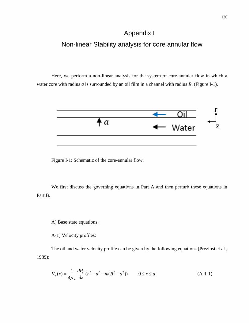
120

Appendix I

Non-linear Stability analysis for core annular flow

Here, we perform a non-linear analysis for the system of core-annular flow in which a

water core with radius a is surrounded by an oil film in a channel with radius R. (Figure I-1).

Figure I-1: Schematic of the core-annular flow.

We first discuss the governing equations in Part A and then perturb these equations in

Part B.

A) Base state equations:

A-1) Velocity profiles:

The oil and water velocity profile can be given by the following equations (Preziosi et al.,

1989):

2 2 2 21( ) ( ( )) 0

4

ww

w

dPV r r a m R a r a

dz (A-1-1)

z

r

121

2 21( ) ( )

4

oo

o

dPV r r R a r R

dz (A-1-2)

where the constant w

o

M

.

The average oil and water velocities can be calculated from Equations A-1-1 and 2:

2

2 20

2

21

( ( ))4 2

a

ww r w

w

w

V r drV dA dP a

V m R aA a dZ

(A-1-3)

2 2

2 2

21 1

( ( ))( ) 4 2

R

oo r a o

o

o

V r drV dA dP

V a RA R a dZ

(A-1-4)

were A is the cross sectional area. Equations A-1-1 and 2 can be re-written in the

following forms based on Equations A-1-3 and 4:

2 2 2 2

22 2

( ) ( )0

( )2

w

w

V r r a m R ar a

aVm R a

(A-1-5)

2 2

2 2

( )

1( )

2

o

o

V r r Ra r R

V a R

(A-1-6)

Equations A-1-5 and 6 can be made dimensionless by using R as the characteristic length

and *

o

UR

as the characteristic velocity:

2 2 2

22

( ) (1 )0

(1 )2

w

w

U r r a m ar a

U am a

(A-1-7)

122

2

2

( ) 11

1( 1)

2

o

o

U r ra r

U a

(A-1-8)

where wU and OU are the dimensionless water and oil velocities. wU and OU are the

dimensionless average water and oil velocities. Also, ~ denotes that the parameter has been made

dimensionless.

A-2) Dimensionless Navier-Stokes and boundary condition:

The Navier-Stokes equations for the oil and the water phases and the stress balance at the

oil-water interface are

1( ) [ ( )]w w w w

w w w

V V dP VV r

t z dz r r r

(A-2-1)

1( ) [ ( )]o o o o

o o o

V V dP VV r

t z dz r r r

(A-2-2)

3

2 3

1 ( ) ( )

 w o

aP

z a z z

aP

(A-2-3)

We now make these equations dimensionless by using R , *W , *

R

W, and

2**

oP W as

the characteristic length, velocity, time and pressure, respectively:

2

*

 1 1( ) ( )

2 Re

ww w wU U Ud P ml r

t z d z r r r

(A-2-4)

*

2  1 1 1( )

2 Re

oo o oU U Ud Pr

t z d z r r r

(A-2-5)

3

2 3*

1  1( ) ( )

 w o

aP

z

a

We aP

z z

(A-2-6)

123

where *

*Re o

o

W R

,

2*

* 1oW RWe

,

w

o

m

, and w

o

l

.

A-3) Integrating the Navier-Stokes equations:

2

0 *

 1 1( ) ( )

2 Re[ ]

wwa

r

w wU U Ud P ml r

t z d z r rdr

rr

(A-3-1)

*

1 2  1 1 1( )

2 Re[ ]

r a

oo o oU U Ud Pr

t z d z rdr

rr

r

(A-3-2)

For simplicity, we drop ~ in the notations. The integrated Navier-Stokes equations are:

2 2 2 2

2*2

2  1 2( ) ( )

2 2 2 2 Re(1 )

2

ww w w

dPa a a m al U l U U

at z dzm a

(A-3-3)

2 2 2

*

21 1 1 1 4( )

2 2 2 2 Re

oo o o

dPa a aU U U

t z dz

(A-3-4)

A-4) Mass conservation:

The mass conservation equations for the two fluids are

2 2( ) ( )w

d dU a a

dz dt (A-3-5)

2 2(1 ) ( )o

d dU a a

dz dt

(A-3-6)

B) Perturbed equations:

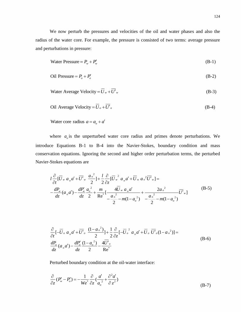
124

We now perturb the pressures and velocities of the oil and water phases and also the

radius of the water core. For example, the pressure is consisted of two terms: average pressure

and perturbations in pressure:

Water Pressure w wP P (B-1)

Oil Pressure o oP P (B-2)

Water Average Velocity w wU U (B-3)

Oil Average Velocity o oU U (B-4)

Water core radius oa a a

where oa is the unperturbed water core radius and primes denote perturbations. We

introduce Equations B-1 to B-4 into the Navier-Stokes, boundary condition and mass

conservation equations. Ignoring the second and higher order perturbation terms, the perturbed

Navier-Stokes equations are

22 2

2 2

2 2*2 2

[ ] [ ]2 2

4 2( ) [ ]

2 Re(1 ) (1 )

2 2

oow w w w wo o

oww w o owo

o o

o o

a ll U a a U U a a U a U

t z

dP dP a U a am aa a U

a adz dzm a m a

(B-5)

22 2

2

*

(1 ) 1[ ] [ (1 )]

2 2

(1 ) 4( )

2 Re

ooo o o o oo o

oo o oo

aU a a U U a a U U a

t z

dP dP a Ua a

dz dz

(B-6)

Perturbed boundary condition at the oil-water interface:

2

* 2 2

  1( ) ( )

 w o

o

Pz We z

a a

z aP

(B-7)

125

Perturbed conservation of mass balances:

2 2w

w o

da dU daU a

dz dz dt

(B-8)

22 (1 ) 2oo o o

da dU o daa U a a

dz dz dt

(B-9)

Equations B-5 and B-6 can be combined by substituting wdP

dz

and odP

dz

from these two

equations in Equation B-7:

2

2*2

2

2 2 2 2 *

3

* 3 2

84

2 2[ ] [ ] [ ]

Re(1 )

2

2 2 8[ ] [ ] [ ] [ ]

1 1 1 1 Re

1 1( )

w w

w ow w w w w

oo o o

o oo oo o o oo o

o o o o

U a UdP aa m

l U a U l U U U aat a z a dz a

m a

U a a U a a dP a aU UU U

t a t z a z dz a a

a a

We z a z

(B-10)

We use the perturbations of the following forms:

expo t ia a kz (B-11)

  υ expw wU t ikz (B-12)

o  υ expoU t ikz (B-13)

where is the dimensionless growth rate, 2

k

is the dimensionless wave number and

is the dimensionless wavelength. After introducing Equations B-11,12 and 13, Equation B-10

becomes

126

2

*2

22 2 2

2 2 2 2 *

3

*

υυ υ ( ) 2

υυ

8 42 ( ) [ ]

Re(1 )

2

2 2 8( )

1 1 1 1 Re

1 1[ ( ) ( )]

υ ( )

www w w

oo

o oo o o oo

o o o

ww w

oo

o

o

o

o

dP Uml U l U ik l U

adzm a

a U a U a dPik U

a a a dz a

a ik ike

k

i

a

l i

k

W

(B-14)

The relation between υoand υw and can be found by substituting Equations B-11,12

and 13 into Equations B-8 and B-9:

(2

)υ 2 ww Uik

(B-15)

2

2

2(υ )

1

oo

o

o

aU

a ik

(B-16)

By substituting Equations B-15 and B-16 into Equation B-14 and ignoring the imaginary

terms, the following dispersion relation can be found for

2 0A B C (B-17)

where the constants A, B, and C are

2

22

1

o

o

aA l

a

(B-18)

2

2* 222 )

28

Re 1 (12

o

ooo

a mB

aa m a

(B-19)

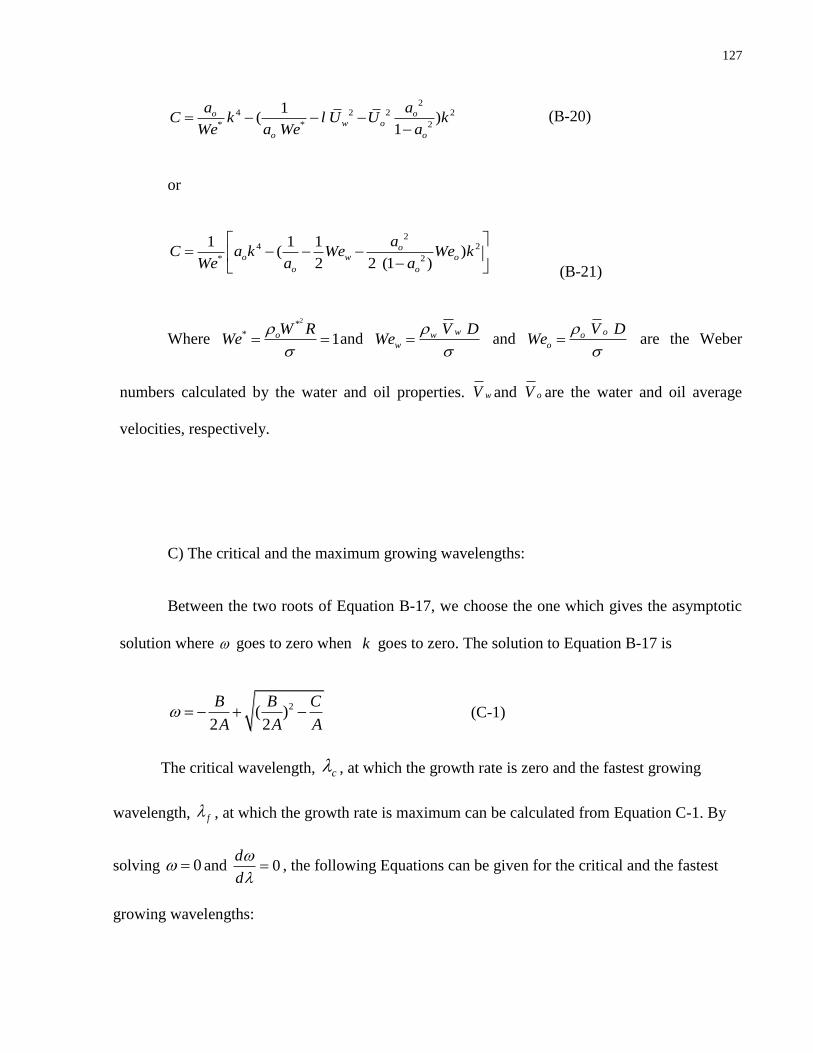
127

4 2 2 22

* * 2

1)(

1

o ow o

o o

a aC k l U U k

aWe We a

(B-20)

or

2

2

*

42

1)

2 2 (

1(

)1

1 oo w o

o o

aC a k We W

We k

ae a

(B-21)

Where

2** 1oWW

Re

and

www

V DWe

and

ooo

V DWe

are the Weber

numbers calculated by the water and oil properties. wV and oV are the water and oil average

velocities, respectively.

C) The critical and the maximum growing wavelengths:

Between the two roots of Equation B-17, we choose the one which gives the asymptotic

solution where goes to zero when k goes to zero. The solution to Equation B-17 is

2( )2 2

B B C

A A A (C-1)

The critical wavelength, c , at which the growth rate is zero and the fastest growing

wavelength, f , at which the growth rate is maximum can be calculated from Equation C-1. By

solving 0 and 0d

d

, the following Equations can be given for the critical and the fastest

growing wavelengths:

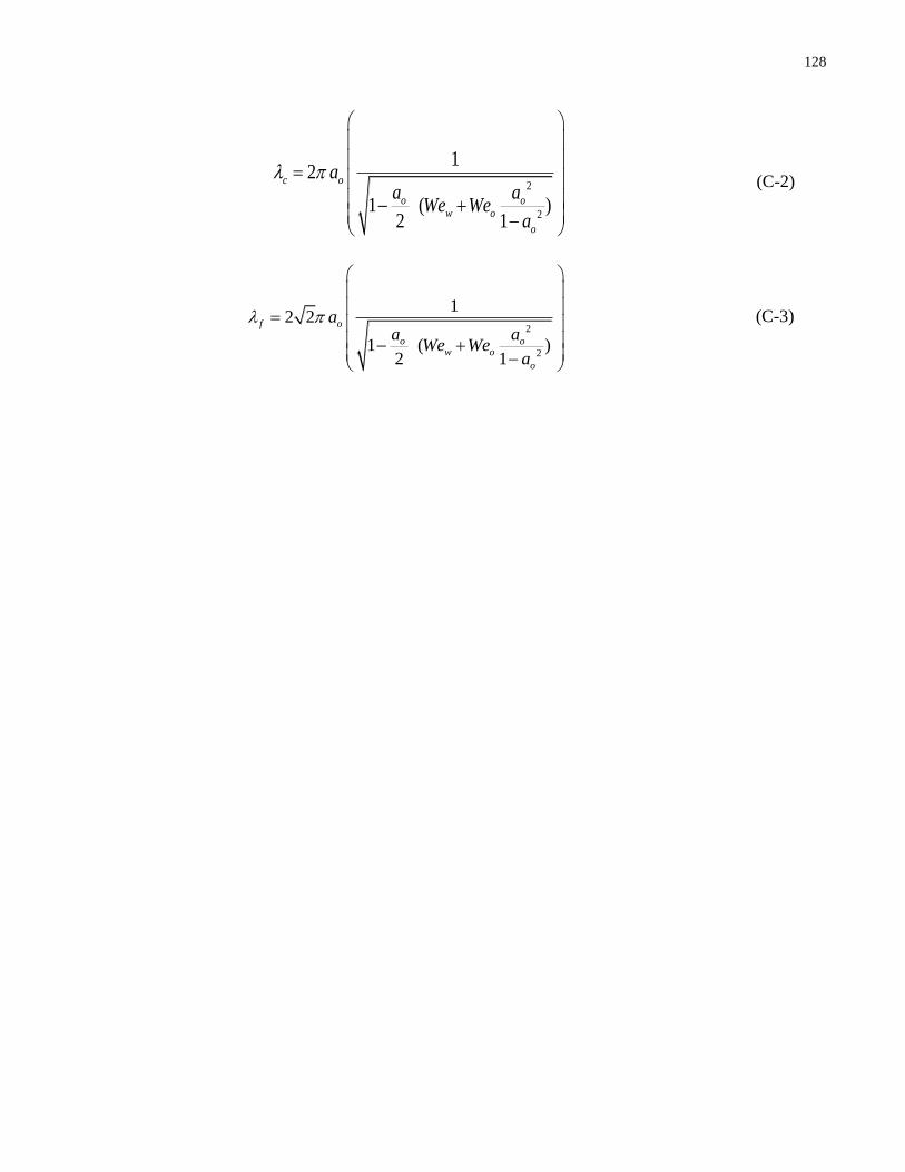
128

2

2

1

1

2

(2

 

)1

c o

o o

o

w o

aa a

aWe We

(C-2)

2

2

1

1 ( )2 1

2 2  f o

o o

o

w o

aa a

aWe We

(C-3)