HAL Id: hal-02995578https://hal-ensta-bretagne.archives-ouvertes.fr/hal-02995578

Submitted on 11 May 2021

HAL is a multi-disciplinary open accessarchive for the deposit and dissemination of sci-entific research documents, whether they are pub-lished or not. The documents may come fromteaching and research institutions in France orabroad, or from public or private research centers.

L’archive ouverte pluridisciplinaire HAL, estdestinée au dépôt et à la diffusion de documentsscientifiques de niveau recherche, publiés ou non,émanant des établissements d’enseignement et derecherche français ou étrangers, des laboratoirespublics ou privés.

Investigation of the Torsional Effects on the LateralBuckling of a Pipe-Like Beam Resting on the Ground

under Axial CompressionPhilippe Le Grognec, Alain Nême, Jie Cai

To cite this version:Philippe Le Grognec, Alain Nême, Jie Cai. Investigation of the Torsional Effects on the LateralBuckling of a Pipe-Like Beam Resting on the Ground under Axial Compression. International Jour-nal of Structural Stability and Dynamics, World Scientific Publishing, 2020, 20 (09), pp.2050110.10.1142/S0219455420501102. hal-02995578

Investigation of the torsional effects on the lateral buckling of a pipe-likebeam resting on the ground under axial compression

Philippe Le Grogneca,∗, Alain Nemea, Jie Caia

aENSTA Bretagne, UMR CNRS 6027, IRDL, F-29200 Brest, France

Abstract

This paper deals with the lateral buckling behavior of an axially compressed beam interacting with the

ground on which it is resting. Such a simple model is supposed to reproduce the same trends as observed

during the lateral buckling of offshore pipelines on the seabed. In such practical analyses, the pipe-soil

interaction relies the ground to the neutral axis of the pipeline. It is shown that, although such a constraint

significantly affects the buckling behavior of the pipeline, it can not reflect the torsional component of the

buckling modes. However, this component is encountered in practice and may further modify the critical

loads. Therefore, in the present preliminary study, the interaction between the beam in hand and the

surrouding ground is modeled by a connection (a continuous distribution of lateral springs) related to the

bottom line of the beam. In this way, the real contact between the soil and the bottom line of a pipe is

mimicked, allowing for both flexural and torsional deformations in the buckling response. The problem is

investigated analytically, using an Euler-Bernoulli beam model with an isotropic linear elastic constitutive

law and also an elastic interaction law. Original analytical solutions are derived and compared to numerical

results obtained through finite element computations. In comparison with classical solutions (with the

connection related to the neutral axis), new types of buckling modes may appear when considering torsional

effects, depending on the boundary conditions, with generally much lower critical loads. These first results

are certainly representative of some features of the global/localized lateral buckling of offshore pipelines,

indicating that torsional effects should also be taken into account in such more comprehensive analyses.

Keywords: Lateral buckling, Torsional effects, Analytical solutions, Numerical simulation, Submarine

pipelines

Nomenclature

Π First Kirchhoff stress tensor

Σ Second Kirchhoff stress tensor

∗Corresponding author.Email address: philippe.le_grognec@ensta-bretagne.fr (Philippe Le Grognec)

Preprint submitted to International Journal of Structural Stability and Dynamics June 18, 2020

Λc Critical stress

ωx Cross-section torsional rotation of the beam

C Fourth-order material tangent elastic reduced tensor

D Fourth-order material tangent elastic tensor

E Green strain tensor

F Deformation gradient

K Fourth-order nominal tangent elastic tensor

U Displacement field

X Bifurcation mode

A Cross-section area of the pipe

E Young’s modulus

Fz Lateral force

G Shear modulus

g Transverse slip along the interface

I Flexural second moment of area of the pipe

J Torsional second moment of area of the pipe

k Stiffness density by unit length of the continuous spring distribution

Kd Discrete lateral stiffness

Mx Torsional moment

Pc Critical force

Re, R External radius of the pipe

Ri Internal radius of the pipe

ux Axial displacement of the centroid axis of the beam

uz Transverse displacement of the centroid axis of the beam

2

1. Introduction

Owing to the growing development and utilization of offshore oil and gas resources, the mechanical

design of offshore pipelines becomes increasingly important. The actual loading conditions coming into play

in the mechanical behavior of submarine pipelines are complex and variable during the entire life cycle of

such structures. The typical loads exerted on pipelines include internal pressure, external pressure, bending5

moments, axial and shear forces (among which frictional forces), and even torsional forces [1]. As a result

of all these conditions, lateral buckling turns out to be one of the main failure modes of such long pipelines

resting on the seabed, and it must be thus particularly investigated for dimensioning purposes.

In practice, the buckling of a pipeline is naturally due to longitudinal compressive stresses that may arise

from various solicitations such as internal and external pressures, but also temperature gradients, among10

others. Indeed, in deep sea environment, high temperatures (HT) and high pressures (HP) are usually

deployed in order to maintain the regular operation of hydrocarbon contents. The temperature of oil and

gas pipelines may be up to 100C above the water environment, while the internal pressure may be higher

than 10 MPa [2, 3]. Under such loading conditions, pipelines are prone to buckle laterally in a global or more

often local way [4, 5] (the possible local failure of pipelines due to extra bending after overall buckling will15

not be discussed in this paper, see [6, 7] for more details on this topic). The considerable length of submarine

pipelines, relatively to their diameter, makes the use of beam models perfectly natural for modeling purposes.

In this framework, the concept of effective axial force has been therefore introduced so as to integrate in a

simplified way the combined effects of the thermal expansion and the internal/external pressures, without

involving any complex integral on the double-curved surface of the pipe due to pressures, what allows one to20

deal easily with global buckling, for instance. For detailed derivations of this controversial but widely used

effective axial force, please refer to researchers such as Palmer and Baldry [8], Fyrileiv and Collberg [9] and

Vedeld et al. [10], or to engineering standards (DNV).

Despite the fact that a pipeline behaves like a slender beam under axial compression, the classical Euler

buckling loads are not suitable, mainly because of the pipe-soil interaction that plays a major role in the25

lateral buckling response. When a pipeline is resting on the seabed, the pipe-soil interaction depends on

many parameters and hence several models have been deployed to date. In traditional pipeline investigation,

typical pipe-seabed models such as the bi-linear [11, 12] and tri-linear [13, 14, 15] models have been developed

and widely used. The soil berm effect has also been included in some research such as [16]. Wang and van

der Heijden [5] made use of a more realistic non-linear pipe-soil interaction model that accounts for the30

effect of lateral breakout resistance. The use of these pipe-seabed models depends on the type of seabed,

which may consist in soft clay [17, 13, 18], stiff clay [16] or sand [19]. In practice, the pipe is supposed to

penetrate into the seabed with a finite depth, giving rise to a finite contact area between the pipe bottom

and the seabed. Wang et al. [20] and Zeng and Duan [21] explicitly investigated this specific configuration,

3

considering the case of a soft seabed. However, for simplicity purposes, the actual uneven seabed is often35

assumed to be flat, without disturbances, also excluding any penetration effect (see Hobbs [22, 23], Taylor

and Gan [2], Ju and Kyriakides [24], Taylor and Tran [25], Karampour et al. [3] and Hong et al. [26], for

instance). The conventional design practice for the pipe-soil interaction assumes thus classically a uniform

frictional behavior in the horizontal direction (proportional to the pipe effective weight underwater, in the

simplest case) [27, 23]. With these simplifications, spring elements shall be used to represent the resistance40

force in the pipe-soil interaction, assuming the seabed to be rigid [28, 11, 29, 19].

To the best of the authors’ knowledge, there are no studies in the literature dealing with the particular

role of torsion in the lateral buckling analysis of submarine pipelines (the spring elements are invariably

connected to the neutral axis of the pipe, and thus the lateral force is applied thereto, so that no torsion is

supposed to occur). In practice, torsional displacements are assumed to be small and torsion is thus ignored45

for pipes with large slenderness in most current research [30, 31]. However, with the assumption of a rigid

seabed and ignoring the pipe embedment, the lateral “frictional” force may rather be applied on the bottom

line of the pipe, in real contact with the seabed, instead of the neutral axis. Under this circumstance, the

torsion effects may have a large influence on the lateral buckling of pipelines and cannot be neglected.

So far, there have been a large number of papers dealing with the lateral buckling of pipelines, aiming50

at predicting critical loads and buckling modes with analytical or numerical models (see [23, 2, 32], among

others). The use of numerical software is clearly interesting as it allows one to include many physical phe-

nomena, without too many simplifications, and to deal with the post-buckling response of pipes, taking

into account both geometric and material non-linearities. Meanwhile, several analytical models have been

recently proposed in the literature for this problem [26, 31], with more or less severe assumptions concerning55

the geometry, constitutive law, loading/boundary conditions and interactions, which bring a more straight-

forward understanding of the lateral buckling phenomenon with more efficient general (mostly closed-form)

solutions.

Therefore, in this paper, a bifurcation analysis of a perfect hollow circular cylindrical tube under axial

compression is carried out, accounting for torsional effects. The lateral (global) buckling is investigated,60

considering an elastic connection between the bottom line of the tube and the ground on which it is laid

down. This specific constraint gives rise to original analytical, possibly closed-form, solutions depending

on the boundary conditions. The paper is organized as follows. In Section 2, use is made of linearized

bifurcation theory so as to solve the buckling problem. This approach is a general and efficient way to

cope with the buckling of structures subjected to uniform pre-critical stress states. Among others, it was65

successfully applied to the cases of compressed homogeneous beams [33], sandwich beam-columns [34, 35]

and two-layer beams with partial interaction (with similar connections) [36, 37], in earlier studies. The

tube is represented by an Euler-Bernoulli beam model with an isotropic linear elastic material, and the

ground-structure interaction is described using a uniform distribution of elastic lateral springs along the

4

beam length, connected to the bottom line of the tube in contact with the soil. The final set of differential70

equations is analytically solved as far as the boundary conditions make it possible. In Section 3, numerical

finite element computations are performed for purposes of comparison with the previous analytical solutions.

The new expressions are also confronted to the solutions obtained without considering torsional effects in

the buckling response. Two sets of boundary conditions are retained and the influence of the stiffness of the

lateral connectors is particularly examined. The results show the importance of torsional effects in such a75

buckling analysis.

2. Analytical study of the lateral buckling of an axially compressed beam

2.1. Problem definition

Let us consider a straight beam, with a hollow circular constant cross-section, resting on the ground. The

bottom line of the cylindrical tube (in contact with the ground) is connected by a continuous distribution80

of lateral springs to the line on the ground representing the initial position of the beam (it means that the

return springs are not stressed in the reference configuration, when the two lines coincide), see Figure 1.

The geometry of the beam is defined by its length L (with endpoints located at x = 0 and x = L) and its

internal and external radii Ri and Re, respectively. Later, use will be made of the cross-section area A, and

the flexural and torsional second moments of area I and J , respectively, which can be expressed in an exact85

form as follows:

A = π(R2e −R2

i

)I =

π(R4e−R

4i )

4

J =π(R4

e−R4i )

2

(1)

The material of the beam is assumed to be homogeneous, isotropic and linear elastic, and the corre-

sponding 3D constitutive law is defined by the fourth-order elasticity tensor D whose components in an

orthonormal basis are Dijkl = λδijδkl + µ (δikδjl + δilδkj), where δij is the Kronecker symbol, and λ and µ

are the Lame constants. Use will be made of the Young’s modulus E (which is related to λ by the standard90

relation λ = Eν(1+ν)(1−2ν) also involving the Poisson’s ratio ν) and the shear modulus G = µ (related to E

and ν by G = E2(1+ν) ). The lateral stiffness density by unit length of the continuous spring distribution,

denoted by k, is supposed to be uniform and constant. There is no need here for a non-linear interaction

law, since only the initial stiffness is involved in the present linearized buckling analysis.

The beam thus defined is subjected to an axial compressive force P which leads to lateral buckling.95

The critical loads and the bifurcation modes are subsequently derived from a 3D framework, using a total

Lagrangian formulation.

5

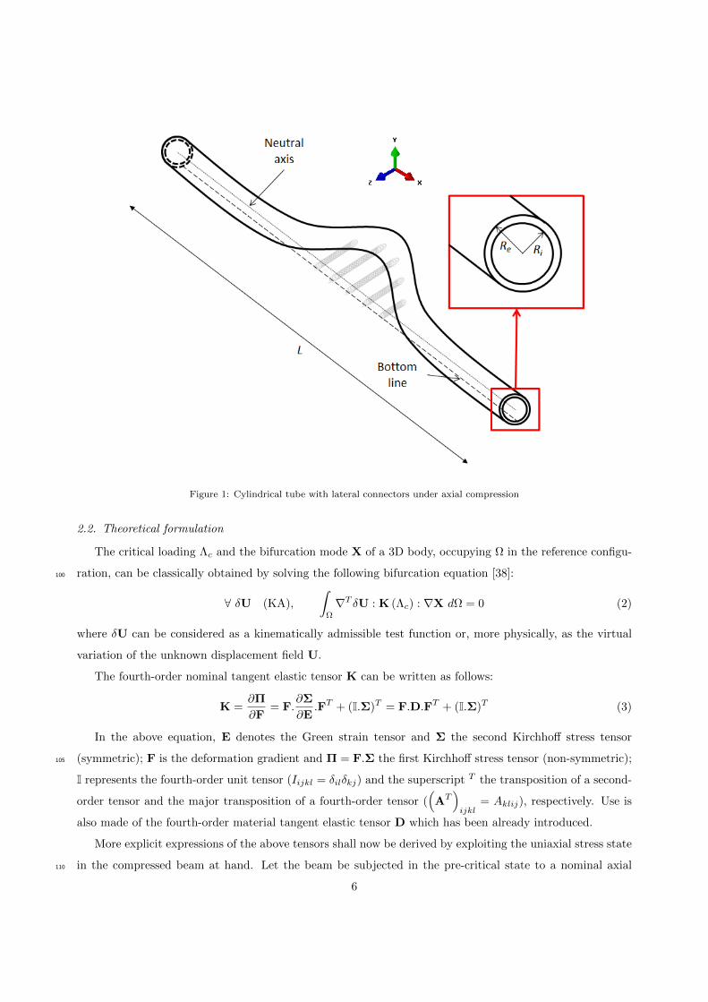
Figure 1: Cylindrical tube with lateral connectors under axial compression

2.2. Theoretical formulation

The critical loading Λc and the bifurcation mode X of a 3D body, occupying Ω in the reference configu-

ration, can be classically obtained by solving the following bifurcation equation [38]:100

∀ δU (KA),

∫Ω

∇T δU : K (Λc) : ∇X dΩ = 0 (2)

where δU can be considered as a kinematically admissible test function or, more physically, as the virtual

variation of the unknown displacement field U.

The fourth-order nominal tangent elastic tensor K can be written as follows:

K =∂Π

∂F= F.

∂Σ

∂E.FT + (I.Σ)T = F.D.FT + (I.Σ)T (3)

In the above equation, E denotes the Green strain tensor and Σ the second Kirchhoff stress tensor

(symmetric); F is the deformation gradient and Π = F.Σ the first Kirchhoff stress tensor (non-symmetric);105

I represents the fourth-order unit tensor (Iijkl = δilδkj) and the superscript T the transposition of a second-

order tensor and the major transposition of a fourth-order tensor ((AT)ijkl

= Aklij), respectively. Use is

also made of the fourth-order material tangent elastic tensor D which has been already introduced.

More explicit expressions of the above tensors shall now be derived by exploiting the uniaxial stress state

in the compressed beam at hand. Let the beam be subjected in the pre-critical state to a nominal axial110

6

compressive stress Πxx = −Λ < 0, so that the first Kirchhoff stress tensor Π is expressed in the orthonormal

basis (ex, ey, ez) as:

Π = −Λex ⊗ ex =

−Λ 0 0

0 0 0

0 0 0

(Λ > 0) (4)

Let us make the assumption that the pre-critical deformations are small, which is usually satisfied in

practice:

‖∇U‖ 1 (5)

Thus, the stress tensor Σ writes:115

Σ = F−1.Π ≈ Π (6)

The nominal tangent elastic tensor in Equation (3) becomes:

K ≈ ∂Σ

∂E+ (I.Σ)T = D− Λei ⊗ ex ⊗ ex ⊗ ei (7)

which is independent of the spatial coordinates (the implicit summation convention on repeated indices is

used with i = x, y, z).

Furthermore, when dealing with 1D models like beams, ad hoc assumptions are usually added in order to

enforce some specific stress state in the body. Namely, the transverse normal material stresses are assumed120

to be zero: Σyy = Σzz = 0. Taking into account these assumptions leads one to replace tensor D with the

reduced tensor C defined as:

Cijkl = Dijkl +Dijyy(DyyzzDzzkl−DzzzzDyykl)+Dijzz(DzzyyDyykl−DyyyyDzzkl)

DyyyyDzzzz−DyyzzDzzyy

(i, j) 6= (y, y), (z, z) (k, l) 6= (y, y), (z, z)(8)

It can be readily checked that tensor C has the major and both minor symmetries. Below, only the

following reduced moduli (and their equivalents obtained by major or minor symmetries) will be needed:

Cxxxx = E Cxyxy = Cxzxz = Cyzyz = µ = G (9)

Eventually, the bifurcation equation (2) of a beam writes in the uniaxial stress case:125

∀ δU (KA),

∫Ω

∇T δU : (C− Λcei ⊗ ex ⊗ ex ⊗ ei) : ∇X dΩ = 0 (10)

As far as a connected beam is concerned, one has to consider the previous integral (Equation (10)) in

the global bifurcation equation together with a special term for the contribution of the connectors, which

will be formulated later.

Let us now consider the bending-twisting problem of the considered beam in the xz-plane (uplift is not

introduced in the model, see Figure 1). Owing to the high slenderness ratio of the designed pipelines in130

practice, transverse shear effects may be negligible, so that the Euler-Bernoulli theory is retained for the

7

beam in hand. The Euler-Bernoulli kinematics is defined here by two scalar displacement fields ux(x) and

uz(x), respectively the axial and transverse displacements of the centroid axis of the beam, and the cross-

section torsional rotation ωx(x) about the same axis (the flexural rotation about the y-axis is directly related

to the transverse displacement field since the cross-sections are supposed to remain orthogonal to the centroid135

axis of the beam after deformation). When the beam buckles from the straight position (the fundamental

solution) to a bent-twisted shape, the expressions for the bifurcation mode X and the displacement variation

δU are both chosen according to the following kinematics:

X =

∣∣∣∣∣∣∣∣∣ux − zuz,x−zωxuz + yωx

δU =

∣∣∣∣∣∣∣∣∣δux − zδuz,x−zδωxδuz + yδωx

(11)

The bifurcation mode gradient then writes:

∇X =

ux,x−zuz,xx 0 −uz,x−zωx,x 0 −ωx

uz,x +yωx,x ωx 0

(12)

and the gradient of the displacement variation takes a similar form.140

The contribution of the connectors in the bifurcation equation involves the (modal) transverse slip g

along the interface, which can be expressed as follows:

g = uz −Reωx (13)

where Re will be further denoted by R for brevity purposes.

The global bifurcation equation then writes:

∀ δU (KA),

∫Ω

∇T δU : (C− Λcei ⊗ ex ⊗ ex ⊗ ei) : ∇X dΩ +

∫ L

0

δg k g dx = 0 (14)

that is to say:145

∀ δux, δuz, δωx (KA),

∫Ω

[E (ux,x−zuz,xx ) (δux,x−zδuz,xx ) + y2Gωx,x δωx,x +z2Gωx,x δωx,x

−Pc

A (ux,x−zuz,xx ) (δux,x−zδuz,xx )− Pc

A z2ωx,x δωx,x

−Pc

A (uz,x +yωx,x ) (δuz,x +yδωx,x )]dΩ +

∫ L0k (uz −Rωx) (δuz −Rδωx) dx = 0

(15)

where the compressive force P = ΛA will act further as the bifurcation parameter.

First, by integrating over the cross-section and eliminating negligible higher-order terms (presupposing

that Λc E,G), the bifurcation equation (15) can be simplified into:

∀ δux, δuz, δωx (KA),∫ L

0[EAux,x δux,x +EIuz,xx δuz,xx +GJωx,x δωx,x

−Pcuz,x δuz,x +k (uz −Rωx) (δuz −Rδωx)] dx = 0(16)

8

Then, integrating by parts with respect to x yields three local differential equations for the components

ux, uz and ωx of the eigenmode:150

EAux,xx = 0

EIuz,xxxx +Pcuz,xx +k (uz −Rωx) = 0

GJωx,xx +kR (uz −Rωx) = 0

(17)

together with the natural boundary conditions, which will be specified later when necessary.

2.3. Solution procedure

The first differential equation in (17) is decoupled from the two others and it leads to the trivial solution

ux = 0 whatever the boundary conditions. The last two equations are coupled with each other, since they

both involve the lateral displacement field uz and the rotation ωx. The sought buckling modes are thus155

prone to combine bending and torsion.

At this stage, in order to facilitate further analysis, a set of dimensionless parameters is defined:

α = IAR2

β = GE

γ = AL2

I

ξ = kR2

EA

P = PEA

(18)

and the last two differential equations in (17) can be re-written as follows:

1γ uz,xxxx +Pcuz,xx +

√αγξ

(√αγuz − ωx

)= 0

2βωx,xx +γξ(√αγuz − ωx

)= 0

(19)

where x = xL is the new dimensionless longitudinal coordinate and the modal displacement uz has been

replaced by the dimensionless field uz = uz

L .160

The equation system (19) will be solved below for two particular choices of boundary conditions: con-

cerning the tranverse displacement, simply-supported conditions will be equally assumed in both cases (as

already considered in many previous studies, such as [39, 40]), whereas the torsional rotation at the ends of

the beam will be either fixed or free. All the subsequent results are applicable, provided that the following

condition is fulfilled (which is always the case in practice):165

ξ < 4αβ2 (20)

2.3.1. Simply-supported conditions without torsional rotation

In the present case, the components of the eigenmode must satisfy the following displacement boundary

conditions at both ends x = 0 and x = 1: uz(0) = 0, uz(1) = 0, ωx(0) = 0 and ωx(1) = 0. The remaining

9

stress boundary conditions stemming from the integration by parts of the bifurcation equation are written

thus: uz,xx (0) = 0 and uz,xx (1) = 0.170

It can be shown that, with the boundary conditions defined above, the modal transverse displacement

takes necessarily the same sinusoidal form as the buckling mode of a single beam under axial compression,

that is to say:

uz = sin(nπx) (21)

where n represents the half-wave number of the mode. The torsional component of the mode is also found to

be sinusoidal (which is naturally consistent with the fixed rotations at the ends) and a closed-form solution175

can be obtained for the corresponding dimensionless critical force (or critical strain):

Pc(n) =n2π2

γ+

αγξ

n2π2 + γξ2β

(22)

which also depends on the half-wave number n of the buckling mode.

From Equation (22), the minimum critical value (corresponding to the first buckling mode) is obtained

by minimizing Pc(n) with respect to the integer n.

2.3.2. Simply-supported conditions with free torsional rotation180

Let us now consider the case with similar simply-supported conditions, as far as bending is concerned,

but free torsional rotation at both ends. In this context, two different mode types are encountered, that are

decoupled from each other. The buckling modes are alternately symmetric and antisymmetric with respect

to the middle of the beam: the antisymmetric modes display a classical sinusoidal shape as obtained before

(with the same critical load), whereas the previous sinusoidal symmetric modes are replaced here by more185

complex solutions involving hyperbolic functions. The existence of such a symmetric mode is guaranteed

once the following conditions are fulfilled:

ξ ≥ ξmin = αβ2

[1−

√1−

(ηχ

)2]2

χ ≥ π2

(23)

where χ =√

αβγ8 and η is the real positive solution of the transcendental equation:

η − sin(2η)

1 +1

2

√1−

(η

χ

)2 = 0 (24)

The first inequality in (23) will be verified in the practical applications, when considering usual values

for the stiffness of lateral connectors, whereas the second inequality is mainly related to the slenderness of190

the pipe and is naturally satisfied for current geometries.

As the first mode is symmetric in practice (combined with the fact that the antisymmetric modes and

corresponding critical loads have been fully described above), one will only be interested here in symmetric

10

modes. Considering now, for simplicity purposes, that the middle of the beam corresponds to the longitudinal

coordinate x = 0, only even functions will be involved in the sought buckling modes. Hence, the general195

symmetric solution of the equation system (19) for the lateral displacement turns out to be in the following

form:

uz = c0 + c1 cosh(ax) cos(bx) + c2 sinh(ax) sin(bx) (25)

where the coefficients c0, c1 and c2 are constants to be defined and the arguments a and b, respectively in the

hyperbolic and sinusoidal functions, can be expressed in terms of the dimensionless parameters as follows:

a = 12√

2

√γβ

√2√

2βξ(2αβ − Pc

)+ ξ − 2βPc

b = 12√

2

√γβ

√2√

2βξ(2αβ − Pc

)+ 2βPc − ξ

(26)

A similar expression (with other coefficients) is obtained for the torsional rotation.200

In this new case, the components of the eigenmode must satisfy the following displacement boundary

conditions at both ends x = − 12 and x = 1

2 : uz(− 12 ) = 0, uz(

12 ) = 0. The remaining stress boundary

conditions stemming from the integration by parts of the bifurcation equation write: uz,xx (− 12 ) = 0,

uz,xx ( 12 ) = 0, ωx,x (− 1

2 ) = 0 and ωx,x ( 12 ) = 0. Since both fields uz and ωx, as well as their derivatives, are

either even or odd functions with respect to x, the boundary conditions can only be written at one end of205

the beam, say at x = 12 .

These three boundary conditions form a linear equation system depending on the three constants c0, c1

and c2. One obtains the critical strain Pc by setting the determinant of this linear equation system to zero,

namely by solving the following characteristic equation:

b[−αγ2ξ + Pcγ

(a2 + b2

)+(a2 + b2

) (3a2 − b2

)]sinh(a)

+a[αγ2ξ + Pcγ

(a2 + b2

)+(a2 + b2

) (a2 − 3b2

)]sin(b) = 0

(27)

where a and b have been already expressed in terms of Pc in Equation (26).210

Equation (27) is transcendental and must be solved numerically. Once the minimum critical strain Pc

satisfying this characteristic equation is known, one can plot the modal transverse displacement uz(x) which

has been explicited using a non-zero solution (c0, c1, c2) of the previous equation system as follows:

uz = 1− 2ab cosh( a2 ) cos( b

2 )+(a2−b2) sinh( a2 ) sin( b

2 )2ab

(cosh( a

2 )2

cos( b2 )

2+sinh( a

2 )2

sin( b2 )

2) cosh(ax) cos(bx)

+(a2−b2) cosh( a

2 ) cos( b2 )−2ab sinh( a

2 ) sin( b2 )

2ab(

cosh( a2 )

2cos( b

2 )2+sinh( a

2 )2

sin( b2 )

2) sinh(ax) sin(bx)

(28)

2.4. Connection with the neutral axis

In the case where the connection to the ground is applied on the neutral axis of the beam, the kinematics215

is the same as before (see Equation (11)) but the transverse slip g is reduced here to the following expression:

g = uz (29)

11

The system of differential equations (17) is thus replaced by:

EAux,xx = 0

EIuz,xxxx +Pcuz,xx +kuz = 0

GJωx,xx = 0

(30)

The first and third differential equations in (30) are decoupled from the others and lead to the trivial

solution ux = 0 and ωx = 0. The last equation only involves uz, so that only flexural buckling is expected

(without torsional effects). Using the same dimensionless parameters as before, this unique equation writes:220

1

γuz,xxxx +Pcuz,xx +αγξuz = 0 (31)

When solving Equation (31), one has necessarily to set the torsional rotation to zero at both ends in

order to satisfy the trivial solution ωx = 0, namely to prevent from a rotation rigid mode. Furthermore,

simply-supported conditions are still considered and the same boundary conditions are used as in Subsection

2.3.1: uz(0) = 0, uz(1) = 0, uz,xx (0) = 0 and uz,xx (1) = 0.

The modal transverse displacement takes the same sinusoidal form as before:225

uz = sin(nπx) (32)

and a closed-form solution is obtained again for the critical strain:

Pc(n) =n2π2

γ+

αγξ

n2π2(33)

which is identical to the solution initially found by Timoshenko and Gere [41], among others.

When comparing expressions (22) and (33), one observes that the critical loads obtained in the case of

a connection with the bottom line of the beam (but without torsional rotation at the ends) are necessarily

lower than the ones obtained in the case of a connection with the neutral axis. However, owing to the very230

low values of the ratio γξ2β encountered in practice, the critical loads will almost coincide between the two

cases.

2.5. Special case with a vanishing connection stiffness density

Before a more general numerical validation of the previous analytical solutions, it could be interesting to

consider the special case of a null stiffness density (k = 0) for which the tube is supposed to behave simply235

like a beam under axial compression. Considering that ξ = 0 in Equations (22) and (33) leads to the same

simplified expression of the critical strain:

Pc(n) =n2π2

γ(34)

This solution is consistent with the well-known critical force of an Euler-Bernoulli simply-supported beam

under axial compression:

Pc(n) =n2π2EI

L2(35)

which is naturally minimum for n = 1.240

12

3. Numerical validation and analysis

3.1. Numerical modeling

In order to reinforce the analytical solutions obtained above for the critical values and buckling modes

under various boundary conditions, finite element computations have been performed using Abaqus software.

Shear-flexible linear (two-node) beam elements in 3D space (B31 in Abaqus) have been retained since Euler-245

Bernoulli beam elements (with cubic Hermite interpolation functions) may not be appropriate for torsional

stability problems due to the approximations in the underlying formulation. The geometric and material

parameters are summarized in Table 1. The whole model and especially the boundary conditions are

represented in Figure 2. Vertical displacements (in y-direction) have been set to zero in the whole beam,

since upheaval of the tube is not permitted. A null lateral displacement (in z-direction) has been enforced250

at both ends so as to conform to the simply-supported boundary conditions and the left end has been fixed

longitudinally in order to avoid any rigid mode. Last, both ends have been prevented (or not) from rotation

about the longitudinal axis of the beam, depending on the considered case.

Length Internal radius External radius Young’s modulus Poisson’s ratio

100 m 145 mm 162 mm 210000 MPa 0.3

Table 1: Geometric and material parameters for the numerical validation

The beam is then related to the ground by specific connector elements. Discrete connectors are applied

at each node of the beam so as to reproduce the theoretically continuous distribution of springs. In practice,255

the discrete stiffness Kd at each node (in N/m) equals the stiffness density by unit length k (in N/m2)

multiplied by the length of each element (between connectors). The beam model is classically represented

by its neutral axis, so that it is more convenient to rely the connectors to this line. Thus, a coupled set of

return springs has been used so as to simulate a single lateral spring connected to the bottom line of the

beam. The linear connection is actually defined through the following stiffness matrix relating the lateral260

force and torsional moment exerted by the ground to the lateral displacement and torsional rotation as

follows: Fz

Mx

=

Kd −KdR

−KdR KdR2

uz

ωx

(36)

In the particular case where the connection is really applied to the neutral axis, Equation (36) must be

replaced by the single relation:

Fz = Kduz (37)

Let us recall that the fundamental criterion that allows one to neglect transverse shear effects in the265

13

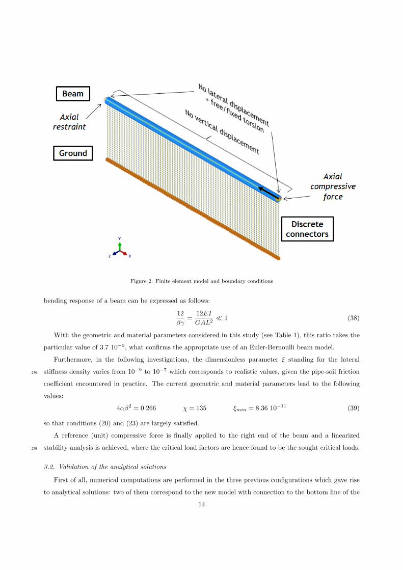
Figure 2: Finite element model and boundary conditions

bending response of a beam can be expressed as follows:

12

βγ=

12EI

GAL2 1 (38)

With the geometric and material parameters considered in this study (see Table 1), this ratio takes the

particular value of 3.7 10−5, what confirms the appropriate use of an Euler-Bernoulli beam model.

Furthermore, in the following investigations, the dimensionless parameter ξ standing for the lateral

stiffness density varies from 10−9 to 10−7 which corresponds to realistic values, given the pipe-soil friction270

coefficient encountered in practice. The current geometric and material parameters lead to the following

values:

4αβ2 = 0.266 χ = 135 ξmin = 8.36 10−11 (39)

so that conditions (20) and (23) are largely satisfied.

A reference (unit) compressive force is finally applied to the right end of the beam and a linearized

stability analysis is achieved, where the critical load factors are hence found to be the sought critical loads.275

3.2. Validation of the analytical solutions

First of all, numerical computations are performed in the three previous configurations which gave rise

to analytical solutions: two of them correspond to the new model with connection to the bottom line of the

14

pipe, with either fixed or free torsional rotation at the ends, and the third one corresponds to the classical

model with connection to the neutral axis. In each case, five particular values of stiffness density have been280

considered, corresponding to ξ = 10−9, 10−8, 4.10−8, 7.10−8, 10−7.

A short mesh sensitivity analysis has been preliminary achieved so as to get converged results and also

verify the ability to reproduce the continuous distribution of springs with discrete connectors (one per

node). For illustration purposes, Table 2 displays the critical forces, in the case of free torsional rotation

with ξ = 10−7, obtained respectively for 25, 50 and 100 elements. A fine mesh of 100 elements of equal285

length (namely 1 m) has been finally retained, in such a way that the discrete stiffness Kd takes the same

value as the stiffness density by unit length k.

Number of elements 25 50 100

Critical force (N) 770516 739349 731581

Table 2: Mesh convergence study

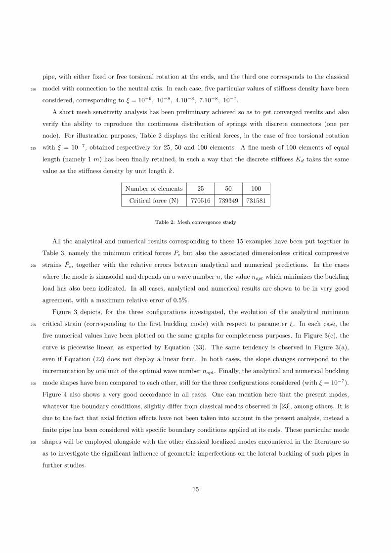
All the analytical and numerical results corresponding to these 15 examples have been put together in

Table 3, namely the minimum critical forces Pc but also the associated dimensionless critical compressive

strains Pc, together with the relative errors between analytical and numerical predictions. In the cases290

where the mode is sinusoidal and depends on a wave number n, the value nopt which minimizes the buckling

load has also been indicated. In all cases, analytical and numerical results are shown to be in very good

agreement, with a maximum relative error of 0.5%.

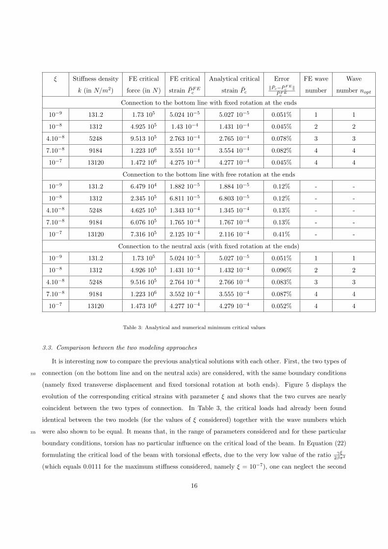
Figure 3 depicts, for the three configurations investigated, the evolution of the analytical minimum

critical strain (corresponding to the first buckling mode) with respect to parameter ξ. In each case, the295

five numerical values have been plotted on the same graphs for completeness purposes. In Figure 3(c), the

curve is piecewise linear, as expected by Equation (33). The same tendency is observed in Figure 3(a),

even if Equation (22) does not display a linear form. In both cases, the slope changes correspond to the

incrementation by one unit of the optimal wave number nopt. Finally, the analytical and numerical buckling

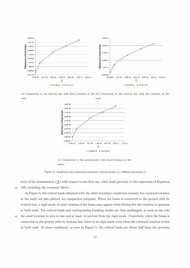
mode shapes have been compared to each other, still for the three configurations considered (with ξ = 10−7).300

Figure 4 also shows a very good accordance in all cases. One can mention here that the present modes,

whatever the boundary conditions, slightly differ from classical modes observed in [23], among others. It is

due to the fact that axial friction effects have not been taken into account in the present analysis, instead a

finite pipe has been considered with specific boundary conditions applied at its ends. These particular mode

shapes will be employed alongside with the other classical localized modes encountered in the literature so305

as to investigate the significant influence of geometric imperfections on the lateral buckling of such pipes in

further studies.

15

ξ Stiffness density FE critical FE critical Analytical critical Error FE wave Wave

k (in N/m2) force (in N) strain PFEc strain Pc‖Pc−PFE

c ‖PFE

cnumber number nopt

Connection to the bottom line with fixed rotation at the ends

10−9 131.2 1.73 105 5.024 10−5 5.027 10−5 0.051% 1 1

10−8 1312 4.925 105 1.43 10−4 1.431 10−4 0.045% 2 2

4.10−8 5248 9.513 105 2.763 10−4 2.765 10−4 0.078% 3 3

7.10−8 9184 1.223 106 3.551 10−4 3.554 10−4 0.082% 4 4

10−7 13120 1.472 106 4.275 10−4 4.277 10−4 0.045% 4 4

Connection to the bottom line with free rotation at the ends

10−9 131.2 6.479 104 1.882 10−5 1.884 10−5 0.12% - -

10−8 1312 2.345 105 6.811 10−5 6.803 10−5 0.12% - -

4.10−8 5248 4.625 105 1.343 10−4 1.345 10−4 0.13% - -

7.10−8 9184 6.076 105 1.765 10−4 1.767 10−4 0.13% - -

10−7 13120 7.316 105 2.125 10−4 2.116 10−4 0.41% - -

Connection to the neutral axis (with fixed rotation at the ends)

10−9 131.2 1.73 105 5.024 10−5 5.027 10−5 0.051% 1 1

10−8 1312 4.926 105 1.431 10−4 1.432 10−4 0.096% 2 2

4.10−8 5248 9.516 105 2.764 10−4 2.766 10−4 0.083% 3 3

7.10−8 9184 1.223 106 3.552 10−4 3.555 10−4 0.087% 4 4

10−7 13120 1.473 106 4.277 10−4 4.279 10−4 0.052% 4 4

Table 3: Analytical and numerical minimum critical values

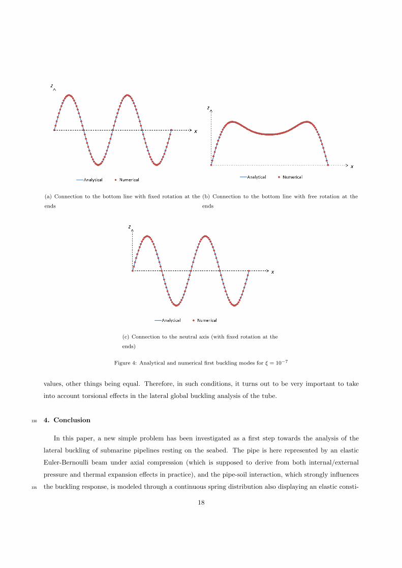
3.3. Comparison between the two modeling approaches

It is interesting now to compare the previous analytical solutions with each other. First, the two types of

connection (on the bottom line and on the neutral axis) are considered, with the same boundary conditions310

(namely fixed transverse displacement and fixed torsional rotation at both ends). Figure 5 displays the

evolution of the corresponding critical strains with parameter ξ and shows that the two curves are nearly

coincident between the two types of connection. In Table 3, the critical loads had already been found

identical between the two models (for the values of ξ considered) together with the wave numbers which

were also shown to be equal. It means that, in the range of parameters considered and for these particular315

boundary conditions, torsion has no particular influence on the critical load of the beam. In Equation (22)

formulating the critical load of the beam with torsional effects, due to the very low value of the ratio γξ2βπ2

(which equals 0.0111 for the maximum stiffness considered, namely ξ = 10−7), one can neglect the second

16

(a) Connection to the bottom line with fixed rotation at the

ends

(b) Connection to the bottom line with free rotation at the

ends

(c) Connection to the neutral axis (with fixed rotation at the

ends)

Figure 3: Analytical and numerical minimum critical strains vs. stiffness parameter ξ

term of the denominator ( γξ2β ) with respect to the first one, what leads precisely to the expression of Equation

(33) excluding the torsional effects.320

In Figure 5, the critical loads obtained with the other boundary conditions (namely free torsional rotation

at the ends) are also plotted, for comparison purposes. When the beam is connected to the ground with its

neutral axis, a rigid mode of axial rotation of the beam may appear when letting free the rotation in question

at both ends. The critical loads and corresponding buckling modes are thus unchanged, as soon as one sets

the axial rotation to zero at one end at least, to prevent from the rigid mode. Conversely, when the beam is325

connected to the ground with its bottom line, there is no rigid mode even when the torsional rotation is free

at both ends. In these conditions, as seen in Figure 5, the critical loads are about half than the previous

17

(a) Connection to the bottom line with fixed rotation at the

ends

(b) Connection to the bottom line with free rotation at the

ends

(c) Connection to the neutral axis (with fixed rotation at the

ends)

Figure 4: Analytical and numerical first buckling modes for ξ = 10−7

values, other things being equal. Therefore, in such conditions, it turns out to be very important to take

into account torsional effects in the lateral global buckling analysis of the tube.

4. Conclusion330

In this paper, a new simple problem has been investigated as a first step towards the analysis of the

lateral buckling of submarine pipelines resting on the seabed. The pipe is here represented by an elastic

Euler-Bernoulli beam under axial compression (which is supposed to derive from both internal/external

pressure and thermal expansion effects in practice), and the pipe-soil interaction, which strongly influences

the buckling response, is modeled through a continuous spring distribution also displaying an elastic consti-335

18

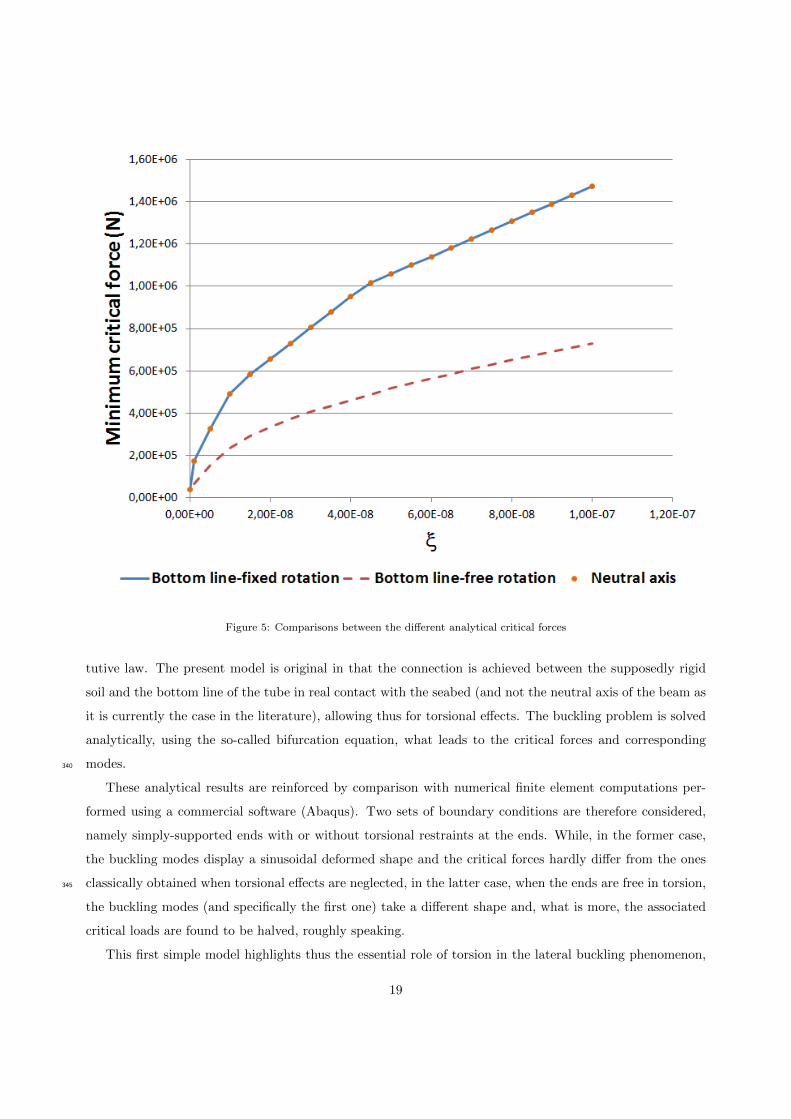
Figure 5: Comparisons between the different analytical critical forces

tutive law. The present model is original in that the connection is achieved between the supposedly rigid

soil and the bottom line of the tube in real contact with the seabed (and not the neutral axis of the beam as

it is currently the case in the literature), allowing thus for torsional effects. The buckling problem is solved

analytically, using the so-called bifurcation equation, what leads to the critical forces and corresponding

modes.340

These analytical results are reinforced by comparison with numerical finite element computations per-

formed using a commercial software (Abaqus). Two sets of boundary conditions are therefore considered,

namely simply-supported ends with or without torsional restraints at the ends. While, in the former case,

the buckling modes display a sinusoidal deformed shape and the critical forces hardly differ from the ones

classically obtained when torsional effects are neglected, in the latter case, when the ends are free in torsion,345

the buckling modes (and specifically the first one) take a different shape and, what is more, the associated

critical loads are found to be halved, roughly speaking.

This first simple model highlights thus the essential role of torsion in the lateral buckling phenomenon,

19

at least under particular boundary conditions. In practice, a more realistic analysis of the lateral buckling

of submarine pipelines requires the use of a more comprehensive model, involving new features such as350

(axial) friction effects [42], material and geometric non-linearities, among other things, but there is no doubt

that torsion will also influence the global/localized buckling response of such practical pipelines. Further

analyses are currently performed in that direction so as to get closer to real conditions, in terms of constitutive

laws, geometric imperfections, boundary conditions and initial conditions (such as residual stresses), still

considering the crucial influence of torsional effects, which should result in a new paper.355

References

[1] Bai, Y., Igland, R. and Moan, T., Tube collapse under pressure, tension and bending loads, International Journal of

Offshore and Polar Engineering 3 Issue 2 (1993) 121–129.

[2] Taylor, N. and Gan, A.B., Submarine pipeline buckling – imperfection studies, Thin-Walled Structures 4 Issue 4 (1986)

295–323.

[3] Karampour, H., Albermani, F. and Gross, J., On lateral and upheaval buckling of subsea pipelines, Engineering Structures

52 (2013) 317–330.

[4] Hunt, G.W. and Blackmore, A., Principles of localized buckling for a strut on an elastoplastic foundation, Journal of

Applied Mechanics 63 Issue 1 (1996) 234–239.

[5] Wang, Z. and van der Heijden, G.H.M., Localised lateral buckling of partially embedded subsea pipelines with nonlinear

soil resistance, Thin-Walled Structures 120 (2017) 408–420.

[6] Cai, J., Jiang, X. and Lodewijks, G., Residual ultimate strength of offshore metallic pipelines with structural damage – a

literature review, Ships and Offshore Structures 12 Issue 8 (2017) 1037–1055.

[7] Cai, J., Jiang, X., Lodewijks, G., Pei, Z. and Wu, W., Residual ultimate strength of damaged seamless metallic pipelines

with combined dent and metal loss, Marine Structures 61 (2018) 188–201.

[8] Palmer, A.C. and Baldry, J.A.S., Lateral buckling of axially constrained pipelines, Journal of Petroleum Technology 26

Issue 11 (1974) 1283–1284.

[9] Fyrileiv, O. and Collberg, L., Influence of pressure in pipeline design: Effective axial force, ASME 24th International

Conference on Offshore Mechanics and Arctic Engineering Halkidiki, Greece, June 12-17, 2005.

[10] Vedeld, K., Sollund, H.A., Hellesland, J. and Fyrileiv, O., Effective axial forces in offshore lined and clad pipes, Engineering

Structures 66 (2014) 66–80.

[11] Galgoul, N.S., Massa, A.L.L. and Claro, C.A., Lateral buckling: Trying to be less conservative, ASME International

Pipeline Conference Calgary, Alberta (Canada), October 4-8, 2004.

[12] Murff, J.D., Wagner, D.A. and Randolph, M.F., Pipe penetration in cohesive soil, Geotechnique 39 Issue 2 (1989) 213–229.

[13] Bruton, D., White, D.J., Cheuk, C.Y., Bolton, M.D. and Carr, M., Pipe/soil interaction behavior during lateral buckling,

including large-amplitude cyclic displacement tests by the safebuck JIP, Offshore Technology Conference Houston, Texas

(USA), May 1-4, 2006.

[14] Schotman, G.J.M. and Stork, F.G., Pipe-soil interaction: A model for laterally loaded pipelines in clay, Offshore Technology

Conference Houston, Texas (USA), April 27-30, 1987.

[15] Zhang, J., Stewart, D.P. and Randolph, M.F., Kinematic hardening model for pipeline-soil interaction under various

loading conditions, International Journal of Geomechanics 2 Issue 4 (2002) 419–446.

[16] White, D.J. and Cheuk, C.Y., Modelling the soil resistance on seabed pipelines during large cycles of lateral movement,

Marine Structures 21 Issue 1 (2008) 59–79.

20

[17] Cheuk, C.Y. and Bolton, M.D., A technique for modelling the lateral stability of on-bottom pipelines in a small drum

centrifuge, 6th International Conference on Physical Modelling in Geotechnics Hong-Kong, August 4-6, 2006.

[18] Cheuk, C.Y., White, D.J. and Bolton, M.D., Large-scale modelling of soil-pipe interaction during large amplitude cyclic

movements of partially embedded pipelines, Canadian Geotechnical Journal 44 Issue 8 (2007) 977–996.

[19] Zhang, Z., Liu, H. and Chen, Z., Lateral buckling theory and experimental study on pipe-in-pipe structure, Metals 9 Issue

2 (2019) 185–200.

[20] Wang, L., Shi, R., Yuan, F., Guo, Z. and Yu, L., Global buckling of pipelines in the vertical plane with a soft seabed,

Applied Ocean Research 33 Issue 2 (2011) 130–136.

[21] Zeng, X. and Duan, M., Mode localization in lateral buckling of partially embedded submarine pipelines, International

Journal of Solids and Structures 51 Issue 10 (2014) 1991–1999.

[22] Hobbs, R.E., Pipeline buckling caused by axial loads, Journal of Constructional Steel Research 1 Issue 2 (1981) 2–10.

[23] Hobbs, R.E., In-service buckling of heated pipelines, Journal of Transportation Engineering 110 Issue 2 (1984) 175–189.

[24] Ju, G.T. and Kyriakides, S., Thermal buckling of offshore pipelines, Journal of Offshore Mechanics and Arctic Engineering

110 Issue 4 (1988) 355–364.

[25] Taylor, N. and Tran, V., Prop-imperfection subsea pipeline buckling, Marine Structures 6 Issue 4 (1993) 325–358.

[26] Hong, Z., Liu, R., Liu, W. and Yan, S., Study on lateral buckling characteristics of a submarine pipeline with a single

arch symmetric initial imperfection, Ocean Engineering 108 (2015) 21–32.

[27] Kerr, A.D., Analysis of thermal track buckling in the lateral plane, Acta Mechanica 30 Issues 1-2 (1978) 17–50.

[28] Miles, D.J. and Calladine, C.R., Lateral thermal buckling of pipelines on the sea bed, Journal of Applied Mechanics 66

Issue 4 (1999) 891–897.

[29] Zhang, X. and Duan, M., Prediction of the upheaval buckling critical force for imperfect submarine pipelines, Ocean

Engineering 109 (2015) 330–343.

[30] Zhu, J., Attard, M.M. and Kellermann, D.C., In-plane nonlinear localised lateral buckling of straight pipelines, Engineering

Structures 103 (2015) 37–52.

[31] Liu, R. and Wang, X., Lateral global buckling high-order mode analysis of a submarine pipeline with imperfection, Applied

Ocean Research 73 (2018) 107–126.

[32] Zhang, X., Soares, C.G., An, C. and Duan, M., An unified formula for the critical force of lateral buckling of imperfect

submarine pipelines, Ocean Engineering 166 (2018) 324–335.

[33] Le Grognec, P. and Le van, A., On the plastic bifurcation and post-bifurcation of axially compressed beams, International

Journal of Non-Linear Mechanics 46 Issue 5 (2011) 693–702.

[34] Douville, M.A. and Le Grognec, P., Exact analytical solutions for the local and global buckling of sandwich beam-columns

under various loadings, International Journal of Solids and Structures 50 Issues 16-17 (2013) 2597–2609.

[35] Le Grognec, P. and Sad Saoud, K., Elastoplastic buckling and post-buckling analysis of sandwich columns, International

Journal of Non-Linear Mechanics 72 (2015) 67–79.

[36] Le Grognec, P., Nguyen, Q.H. and Hjiaj, M., Exact buckling solution for two-layer Timoshenko beams with interlayer slip,

International Journal of Solids and Structures 49 Issue 1 (2012) 143–150.

[37] Le Grognec, P., Nguyen, Q.H. and Hjiaj, M., Plastic bifurcation analysis of a two-layer shear-deformable beam-column

with partial interaction, International Journal of Non-Linear Mechanics 67 (2014) 85–94.

[38] Nguyen, Q.S., Stability and Non-Linear Solid Mechanics (Wiley, 2000).

[39] Karampour, H., Albermani, F. and Major, P., Interaction between lateral buckling and propagation buckling in tex-

tured deep subsea pipelines, ASME 34th International Conference on Ocean, Offshore and Arctic Engineering St. John’s,

Newfoundland, Canada, May 31-June 5, 2015.

[40] Karampour, H., Effect of proximity of imperfections on buckle interaction in deep subsea pipelines, Marine Structures 59

21

(2018) 444–457.

[41] Timoshenko, S.P. and Gere, J.M., Theory of Elastic Stability (Mc Graw-Hill, 1961).

[42] Wang, Z., van der Heijden, G.H.M. and Tang, Y., Localised upheaval buckling of buried subsea pipelines, Marine Structures

60 (2018) 165–185.

22