Investigation of The Distribution and Fe Content of Iron

Volume 9. Issue 1. 141-160 APRIL 2020

Jurnal Ilmiah Pendidikan Fisika Al-BiRuNi https://ejournal.radenintan.ac.id/index.php/al-biruni/index

DOI: 10.24042/jipfalbiruni.v9i1.5394

P-ISSN: 2303-1832

e-ISSN: 2503-023X

Investigation of The Distribution and Fe Content of Iron Sand at Wari

Ino Beach Tobelo Using Resistivity Method with Werner-Schlumberger

Configuration

Bayu Achil Sadjab1*, I Putu Tedy Indrayana2, Steven Iwamoni3, Rofiqul Umam4

1, 2 Physics Study Program, Faculty of Natural Science and Engineering Technology, Universitas Halmahera, Maluku

Utara, Indonesia. 3 Environmental Agency of Kabupaten Halmahera Utara, Maluku Utara, Indonesia 4 Faculty of Science and Technology, Kwansei Gakuin University, Hyogo, Japan

*Corresponding Address: [email protected]

Article Info ABSTRACT Article history:

Received: December 7th, 2019

Accepted: April 24th, 2020 Published: April 30th, 2020

This research aimed to investigate the distribution, volume, and concentration of iron sand at Wari Ino Beach Tobelo. The resistivity method with Werner-Schlumberger configuration was applied to investigate the iron sand distribution. The measurements were set-up on 3 lines that run parallel along the coast of Wari Ino Village. The length of each trajectory was 150 meters with a spacing of 10 meters for each electrode. Data acquisition was

carried out by using geoelectric instruments to obtain current injec tion (I) and voltage (V). The analysis was carried out by using RES2DINV and ROCKWORK software to obtain 2-D and 3-D cross-section models for interpreting the distribution and volume of the iron sand. The analysis and interpretation were supported by geological data of the location. Furthermore, the Fe content was characterized by using X-Ray Fluorescence

Spectroscopy (XRF). There results show that the volume of the iron sand in each trajectory was 109,355 m3; 180,254 m3; and 120,556 m3. The total volume of iron sand along the three trajectories was up to 405,335 m 3 . The Fe content in the form of a free element is 67.41%, 57.12%, and 73.40%. The Fe content in the form of hematite mineral (Fe2O3) was 57.92%, 45.82%, and 65.47%.

Keywords:

Distribution;

Fe content; Iron sand; Resistivity;

Werner-Schlumberger

© 2020 Physics Education Department, UIN Raden Intan Lampung, Indonesia.

INTRODUCTION

Iron sand contains abundant Fe element

in the form of iron oxide minerals, i.e.

magnetite (Fe3O4), hematite (α-Fe2O3), and

maghemite (γ-Fe2O3). Other minerals such

as Aluminum oxide (Al2O3), Silica dioxide

(SiO2), Phosphorus pentaoxide (P2O5),

Calcium oxide (CaO), Titanium dioxide

(TiO2), Vanadium pentaoxide (V2O5),

Chromium (III) oxide (Cr2O3), and

Manganese oxide (MnO) also have been

investigated exist in the iron sand(Malega et

al., 2018). Generally, the primary minerals

contained in the iron sand are Magnetite

(Fe3O4), Hematite (Fe2O3), Goethite

(Fe2O3.H2O), Siderite (FeCO3) and Pyrite

(FeS2)(Lawan et al., 2018). Those minerals

can be separated into a pure monophase

mineral for the specific applications. Hence,

they have high economic value and impact

on the development of the mining industry

in Indonesia.

The fabricated iron minerals in the form

of iron metal and steel are very useful for

many applications, such as fabrication of

components for electronic devices,

manufacturing, construction sector,

building, vehicles industry as well as for the

automotive sector. According to (The

Indonesia Iron and Steel Industry

https://ejournal.radenintan.ac.id/index.php/al-biruni/index

http://issn.pdii.lipi.go.id/issn.cgi?daftar&&&&&2303-1832

142 Jurnal Ilmiah Pendidikan Fisika Al-BiRuNi, 9 (1) (2020) 141-160

Association, 2017), Indonesia has been

experienced an increasing domestic steel

consumption were 12.70 million tons in

2016 and projected to be 16.00; 17.00;

18.00; 19.10; 20.20; and 21.40 million tons

in 2020 to 2045 in its year in ASEAN,

Indonesia has the lowest steel consumption

In 2020, Indonesia's steel consumption is

predicted achieving of 84 kg/capita that

lower than ASEAN steel consumption about

157 kg/capita. This increase in steel

consumption throughout its multiplier effect

should be concerned by the government of

Indonesia.

In a different case, the synthesized iron

sand in the form of iron oxide into any kind

of nano-materials also has a high economic

impact. The synthesis of nanomaterials from

iron sand is the basis for manufacturing new

types of functional materials to support

advance technologies, such as MRI contrast

agent, drug delivery agent, biosensor optic,

magnetic sensor, catalyst material, nano-

adsorbent, antimicrobial, anticancer

materials, as well as nano-imaging probe

(Bolívar & González, 2019; Dang et al.,

2018; Rahimnia et al., 2019; Sardana et al.,

2018).

Many researchers in Indonesia have

developed nanomaterials based on local iron

sand, for instance nanocomposite based iron

oxide materials as an absorbent of the heavy

metals (Azmiyawati et al., 2017; Rahmawati

et al., 2017; Ramelan et al., 2016; Rettob,

2019; Sebayang et al., 2018; Setiadi et al.,

2016; Putri et al., 2019). The Fe3O4 based

nanocomposite material has fabricated for

nuclear radiating shielding (Dahlan et al.,

2018; Haryati & Dahlan,s 2018). The

nanocomposite of Fe3O4/PEG-4000 by

(Arista et al., 2019) has aplicated for

antibacterial material againts Escherichia

Coli and Staphylococcus aureus. The Fe3O4

nanoparticles have also applied for ink

powder (Fahlepy et al., 2018). Other

researchers also synthesized nanomaterials

based on iron sand for other various

applications, for example magnetic thin film

(Rianto et al., 2018; Yulfriska et al., 2018);

electromagnetic wave absorbing material

(Yusmaniar et al., 2018); heat transfer

application (Imran et al., 2018); catalyst

material (Maulinda et al., 2019); and

magnetic nano-pigment (Yulianto et al.,

2019).

Therefore, the exploration of the iron

sand is very important for the development

of the iron sand industry in Indonesia in the

future. Indonesia has a lot of iron sand sites

where they can be explored to be able

supplying the iron sand raw material. The

iron sand industry will be a future strategic

and potential sector for Indonesia as the last

detail explanation.

Many iron sand deposits belonged by

Indonesia are distributed over all sites inits

region, such as Buaya River Deli Serdang

North Sumatra (Setiadi et al., 2016), Talang

Mountain West Sumatra (Pratiwi et al.,

2017), WediIreng Beach Banyuwangi East

Java (Taufiq et al., 2017), Marina Beach,

Semarang (Azmiyawati et al., 2017), Bugel

Beach, Kulon Progo (Fahmiati et al., 2017),

Betaf Beach, Sarmi Regency Jayapura

(Dahlan et al., 2018; Haryati & Dahlan,

2018), Cemara Sewu Beach Cilacap Central

Java (Nurrohman & Pribadi, 2018),

Sampulungan Beach, Taklar Regency South

Sulawesi (Arsyad et al., 2018), and

Lampanah-Lengah village, District of Aceh

Besar (Adlim et al., 2019).

In addition, Pusat Sumber Daya Geologi

(PSGD) Ministry of Energy and Mineral

Resources has reported in 2013 that there

are 67 sites where the iron sand distributed

in Indonesia (Suprapto & Sunuhadi, 2014).

There are many sites elsewhere the iron

sand deposits not explored yet, for an instant

a site at Wari Ino Beach, Tobelo Halmahera

Utara. A pilot study by (Malega et al., 2018)

had conducted only for identifying the

minerals contained in iron sand at Wari Ino

Beach by using X-Ray Fluorescence (XRF)

Spectroscopy method. The research reported

that the concentration of Fe mineral is about

87.5% of the iron sand mass.

Up to the date no publication provides

information about the distribution and

Jurnal Ilmiah Pendidikan Fisika Al-BiRuNi, 9 (1) (2020) 141-160 143

volume of the iron sand in Wari Ino Beach.

Consequently, we investigated the

distribution and volume of the iron sand in

this site. By knowing the distribution,

volume, and Fe content will allow further

researchers to do exploration and also being

a database for local government, especially

the Department of Natural Resources, Mines

and Energy, Maluku Utara for further iron

sand industry strategic plan in Halmahera

Utara.

The distribution and volume of the iron

sand can be estimated by geophysical

techniques, i.e., Magnetic techniques,

Gravity techniques, Magnetotelluric

technique, Induced-Polarization technique,

and Electrical Resistivity techniques. The

magnetic technique is the oldest geophysical

techniques which measure deposit of the

iron sand based on the variation in the

susceptibility. Gravity techniques to

measure density contrast between minerals

and surrounding rocks. The magnetotelluric

technique measures electrical conductivity

of the iron sand. Those three techniques are

classified into a passive technique based on

signal propagation via investigated minerals

or rocks (Adewuyi & Ahmed, 2019). Hence,

signal is not required to penetrate the iron

sand deposit.

In other hands, Induced-Polarization

technique measures the volume and the

distribution of the iron sand based on the

value of their capacitance. Electrical

Resistivity technique measures electrical

conductivity of iron sand. These two

techniques are classified into active

technique which signal directly penetrate the

iron sand deposit (Adewuyi & Ahmed,

2019). Among those techniques, Electrical

Resistivity technique is the most applied for

the investigation of the distribution and

volume of iron sand deposit.

According to a research paper by (Sehah

et al., 2018), the distribution and volume of

the iron ore in Eastern Binangun Coastal

Cilacap. Those data were interpreted base

on the resistivity data obtained by using

Werner configuration. Another paper by

(Raharjo & Sehah, 2018) had reported the

distribution of the iron sand in the western

coastal area of Nusawungu, Cilacap

Regency by applying the resistivity method

with Schlumberger configuration. The

results showed that the iron sand deposits

are at depths of 2.39-25.25 meters with

resistivity values of 12.24-46.96 Ωm.

Werner configuration is only suitable for

survey mapping of the iron sand distribution

along the horizontal trajectory, but no more

information about a sounding on the vertical

direction. On the other hand, Schlumberger

configuration is only suitable for identifying

the vertical configuration of the iron sand

(Raharjo & Sehah, 2018; Sehah et al.,

2018).

In this research, we applied the Werner-

Schlumberger configuration due to the

configuration to find out the information

both mapping and sounding of the iron sand

volume and distribution under the surface

instantaneously as explained by (Akmam et

al., 2019; Jamaluddin & Umar, 2018). We

have been successfully obtained the 2-D

cross-section contour of lower rock surface

resistivity along the trajectories. In addition,

we also obtained the Pseudo 3-D cross-

sectional area of iron sand in the trajectories.

These results are potentially useful for

further consideration in exploring iron sand

at Wari Ino Beach.

METHODS

Resistivity Method

The geoelectric method can be used well

if there is a resistivity contrast between

mediums. Contrast can be a medium that is

relatively conducive to a non-conductive

medium, or there are lithological

differences. Each type of rock subsurface

has different resistivity values. Each

resistivity depends on the density, moisture

content, minerals, salt content, and rock

porosity (Sehah et al., 2018). The work of

the geoelectric method is by flowing direct

current or alternating low frequency into the

earth medium through two current

electrodes, then measuring the potential


difference arising through the two potential

electrodes. (Naveen et al., 2015)explained

that the distance between the electrodes can

vary according to the area specification and

the topography, so that the resistivity value

can be calculated through Ohm's law.

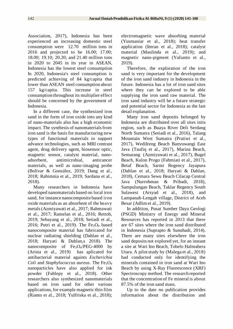
Suppose that R is the resistance (Ohm); A is

the cross-sectional area of the medium (m 2),

and L is the length of the medium (m), then

according to Figure 1, the resistivity of the

medium, ρ (Ωm) can be determined by using

equation 1,

L

AR= (1)

According to Ohm’s law that the resistance

R of the medium mathematically can be

calculated by using equation 2, such as

I

VR

= (2)

Following the potential difference between

edges of the medium ∆V and the injected

current I, so the resistivity can be calculated

by equation 3,

L

A

I

V=

(3)

Figure 1. Samples of the medium through which current I, length L, and cross-sectional area A.

Equation 3 applies to a homogeneous

medium, so the result obtained is true

resistivity. But in practice, the object

measured is the earth or soil that is not

homogeneous because of different types of

resistors, so that the measured resistivity is

apparent resistivity. The apparent resistivity

value depends on the resistivity of the layers

forming the formation and the configuration

of the electrodes used. Pseudo resistivity

ρais formulated by equation 4,

I

VΔKρa = (4)

Where K is the geometrical factor.

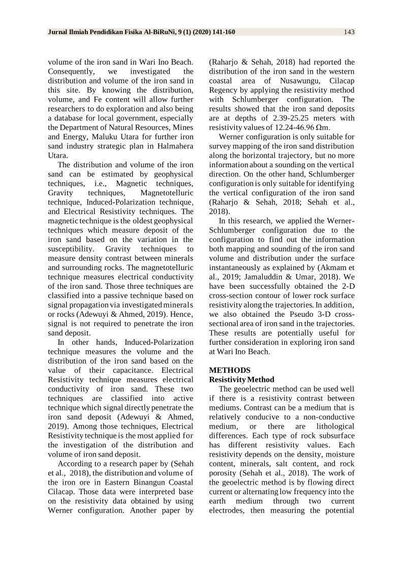
Wenner-Schlumberger Configuration

The Wenner-Schlumberger configuration

is a configuration with a constant spacing

system with a note that the comparison

factor n for this configuration is the ratio of

the distance between the current electrode

(AB) and the potential (MN). If the potential

electrode distance MN is a distance of the

AB electrode is (2na + a) (Figure 2).

This configuration is a combination of

the Wenner configuration and the

Schlumberger configuration. In

measurements with a space factor n = 1, the

Wenner-Schlumberger configuration is the

same as the measurement in the Wenner

configuration (distance between electrodes =

a), but in measurements with n = 2 and so

on, the Wenner-Schlumberger configuration

is the same as the Schlumberger

configuration (the distance between current

electrode and potential electrode are greater

than the distance between potential

electrodes).


The Wenner-Schlumberger configuration

has a penetration depth of up to one-third of

the distance between C1 and C2.

Commonly, the average penetration depth is

up to 90 meters and Wenner configuration

only reaches 80 meters. Variable n is

multiple to show the observed layer's layers.

The geometry factors of the Wenner-

Schlumberger can be calculated by using

equation 5,

( )anπK 1+= (5)

where𝑎 is the distance between the

electrodes P1 and P2, n is the ratio between

the electrode distances C1-P1 and P1-P2 (e.g

4a, then n = 4) so that the resistivity value of

all obtained from the measurement results is

equal to equation 6,

( )I

VΔanπρa 1+= (6)

Generally, rock resistivity values have been

obtained through various direct

measurements and can be used as a

reference in interpreting the results of field

resistivity measurements; this is because

certain resistivity values will be associated

with geological conditions in the

measurement area (Table 1).

Figure 2. The Wenner-Schlumberger configuration

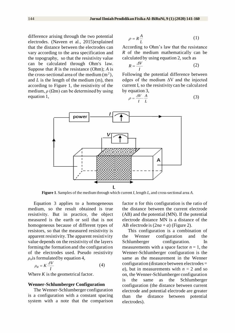
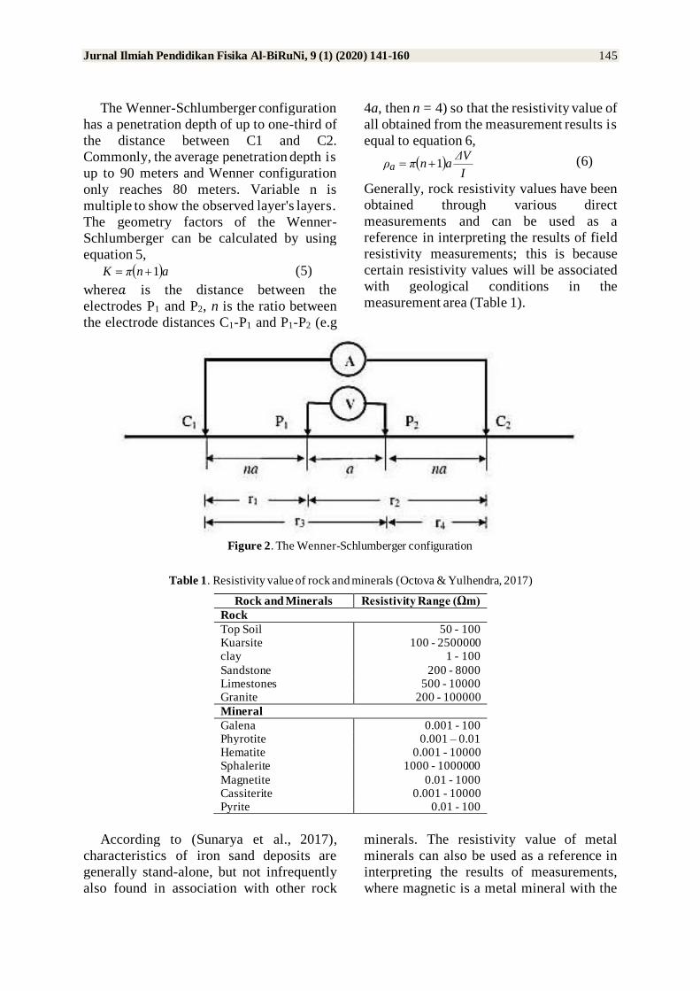
Table 1. Resistivity value of rock and minerals (Octova & Yulhendra, 2017)

Rock and Minerals Resistivity Range (Ωm)

Rock

Top Soil 50 - 100

Kuarsite 100 - 2500000

clay 1 - 100

Sandstone 200 - 8000

Limestones 500 - 10000

Granite 200 - 100000

Mineral

Galena 0.001 - 100

Phyrotite 0.001 – 0.01

Hematite 0.001 - 10000

Sphalerite 1000 - 1000000

Magnetite 0.01 - 1000 Cassiterite 0.001 - 10000 Pyrite 0.01 - 100

According to (Sunarya et al., 2017),

characteristics of iron sand deposits are

generally stand-alone, but not infrequently

also found in association with other rock

minerals. The resistivity value of metal

minerals can also be used as a reference in

interpreting the results of measurements,

where magnetic is a metal mineral with the

https://trisusantosetiawan.files.wordpress.com/2011/01/ws.jpg


highest Fe content, but the amount is small

while hematite is the most needed iron

mineral in the iron industry.

Technical Procedures

The research was conducted by direct

observation and measurement in the field.

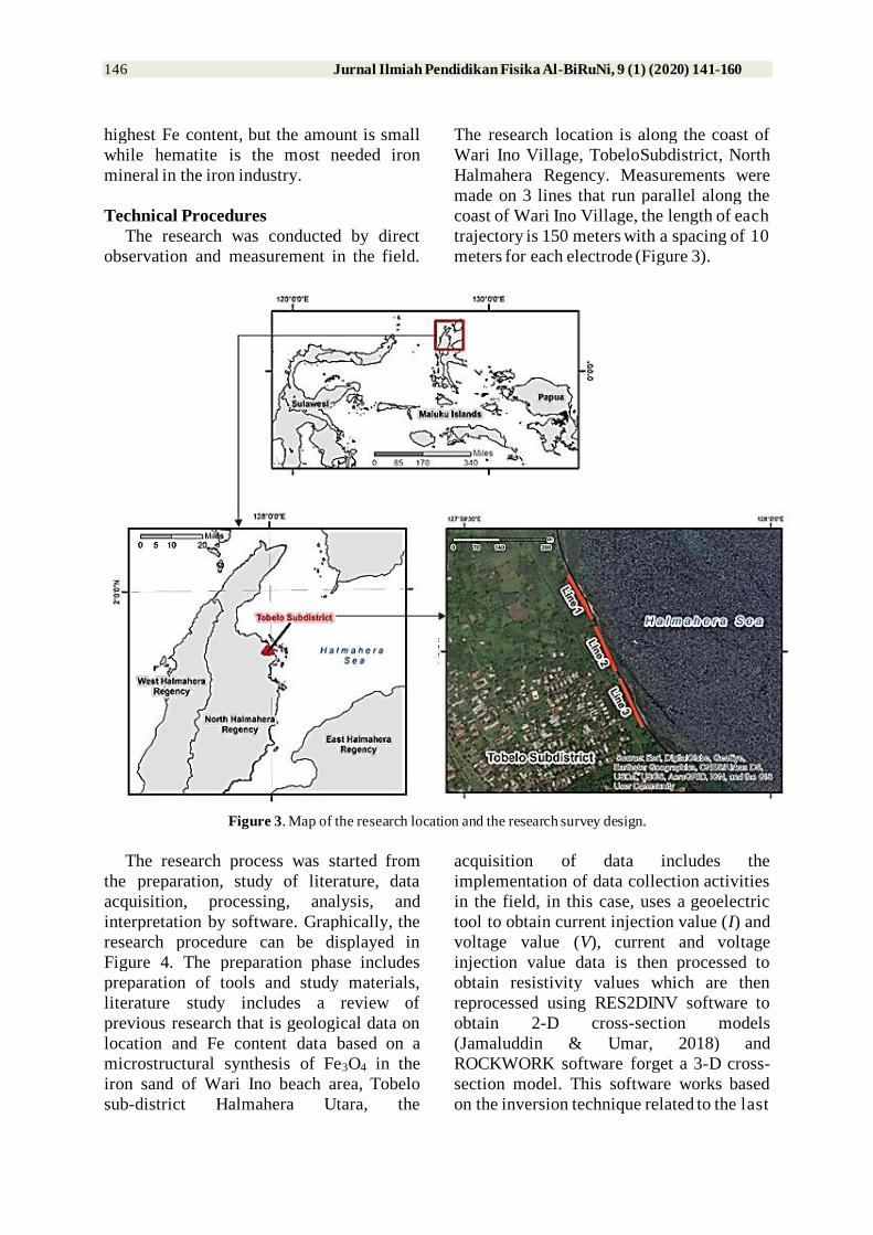
The research location is along the coast of

Wari Ino Village, TobeloSubdistrict, North

Halmahera Regency. Measurements were

made on 3 lines that run parallel along the

coast of Wari Ino Village, the length of each

trajectory is 150 meters with a spacing of 10

meters for each electrode (Figure 3).

Figure 3. Map of the research location and the research survey design.

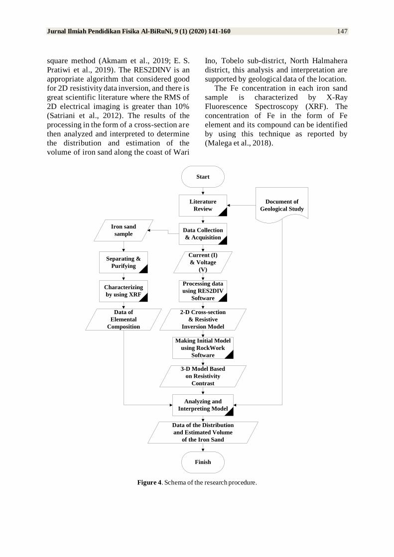
The research process was started from

the preparation, study of literature, data

acquisition, processing, analysis, and

interpretation by software. Graphically, the

research procedure can be displayed in

Figure 4. The preparation phase includes

preparation of tools and study materials,

literature study includes a review of

previous research that is geological data on

location and Fe content data based on a

microstructural synthesis of Fe3O4 in the

iron sand of Wari Ino beach area, Tobelo

sub-district Halmahera Utara, the

acquisition of data includes the

implementation of data collection activities

in the field, in this case, uses a geoelectric

tool to obtain current injection value (I) and

voltage value (V), current and voltage

injection value data is then processed to

obtain resistivity values which are then

reprocessed using RES2DINV software to

obtain 2-D cross-section models

(Jamaluddin & Umar, 2018) and

ROCKWORK software forget a 3-D cross-

section model. This software works based

on the inversion technique related to the last


square method (Akmam et al., 2019; E. S.

Pratiwi et al., 2019). The RES2DINV is an

appropriate algorithm that considered good

for 2D resistivity data inversion, and there is

great scientific literature where the RMS of

2D electrical imaging is greater than 10%

(Satriani et al., 2012). The results of the

processing in the form of a cross-section are

then analyzed and interpreted to determine

the distribution and estimation of the

volume of iron sand along the coast of Wari

Ino, Tobelo sub-district, North Halmahera

district, this analysis and interpretation are

supported by geological data of the location.

The Fe concentration in each iron sand

sample is characterized by X-Ray

Fluorescence Spectroscopy (XRF). The

concentration of Fe in the form of Fe

element and its compound can be identified

by using this technique as reported by

(Malega et al., 2018).

Start

Literature

Review

Data Collection

& Acquisition

Processing data

using RES2DIV

Software

Document of

Geological Study

Current (I)

& Voltage

(V)

2-D Cross-section

& Resistive

Inversion Model

Making Initial Model

using RockWork

Software

3-D Model Based

on Resistivity

Contrast

Analyzing and

Interpreting Model

Data of the Distribution

and Estimated Volume

of the Iron Sand

Finish

Iron sand

sample

Characterizing

by using XRF

Separating &

Purifying

Data of

Elemental

Composition

Figure 4. Schema of the research procedure.


RESULTS AND DISCUSSION

Geology of Research Location

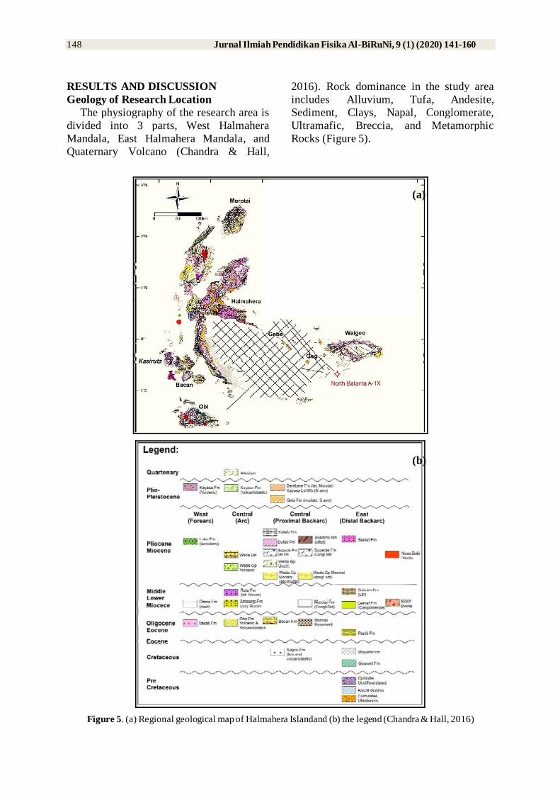
The physiography of the research area is

divided into 3 parts, West Halmahera

Mandala, East Halmahera Mandala, and

Quaternary Volcano (Chandra & Hall,

2016). Rock dominance in the study area

includes Alluvium, Tufa, Andesite,

Sediment, Clays, Napal, Conglomerate,

Ultramafic, Breccia, and Metamorphic

Rocks (Figure 5).

Figure 5. (a) Regional geological map of Halmahera Islandand (b) the legend (Chandra & Hall, 2016)

(a)

(b)


The stratigraphy of the study area

consists of 17 formations composed of age

ranges before the Cretaceous to the

Holocene. The rock structure consists of

Sedimentary Rocks with Dodaga Formation

(Kd), Limestone Unit, Dogosagu Formation

(Tped), Conglomerate Unit (Tpec), Tutuli

Formation (Tomt), Conglomerate (Tmpc),

Tingteng Formation (Tmpt), Vedic

Formation (Tmpw), and Reef Limestone

(Ql). Surface Deposition is with Alluvium

and Coastal Deposition (Qa). GunungApi

Rock with the composition of Bacan

Formation (Tomb), Kayasa Formation

(Qpk), Unit Tufa (Qht), MountApi

Holocene Rock (Qhv). The igneous rocks

are composed of Ultrabasic Rock (Ub),

Gabro (Gb), and Diorite (Di) (Figure 5).

The Distribution of Iron Sand

Measurement data of observations were

obtained a current (I), voltage (∆V),

apparent resistivity (ρ), datum point data,

spaces, number of layers. The processing by

RES2DINV software for the three

trajectories that run parallel along the coast

of Wari Ino village. The results of 2-D

inversion then saved into a format (.xyz).

Data with the format (.xyz) consists of the

accumulation of electrode distances,

resistivity values, depth of current

penetration, and subsurface conductivity

based on measurement results.

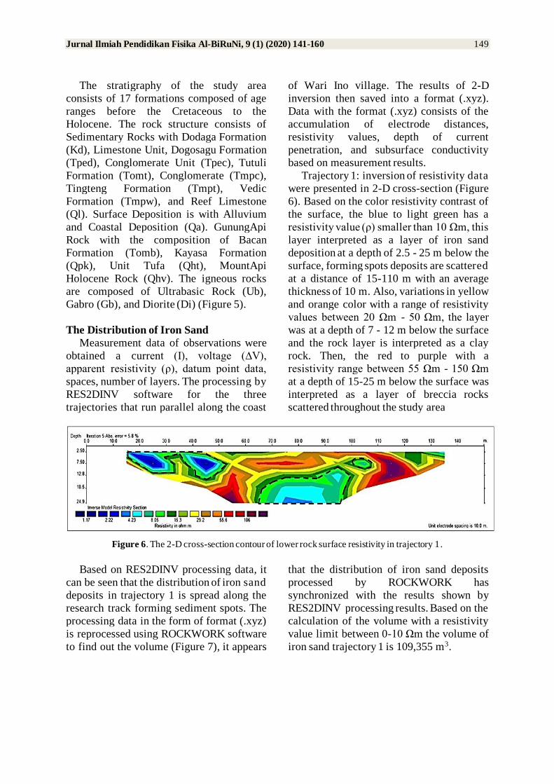
Trajectory 1: inversion of resistivity data

were presented in 2-D cross-section (Figure

6). Based on the color resistivity contrast of

the surface, the blue to light green has a

resistivity value (ρ) smaller than 10 Ωm, this

layer interpreted as a layer of iron sand

deposition at a depth of 2.5 - 25 m below the

surface, forming spots deposits are scattered

at a distance of 15-110 m with an average

thickness of 10 m. Also, variations in yellow

and orange color with a range of resistivity

values between 20 Ωm - 50 Ωm, the layer

was at a depth of 7 - 12 m below the surface

and the rock layer is interpreted as a clay

rock. Then, the red to purple with a

resistivity range between 55 Ωm - 150 Ωm

at a depth of 15-25 m below the surface was

interpreted as a layer of breccia rocks

scattered throughout the study area

Figure 6. The 2-D cross-section contour of lower rock surface resistivity in trajectory 1.

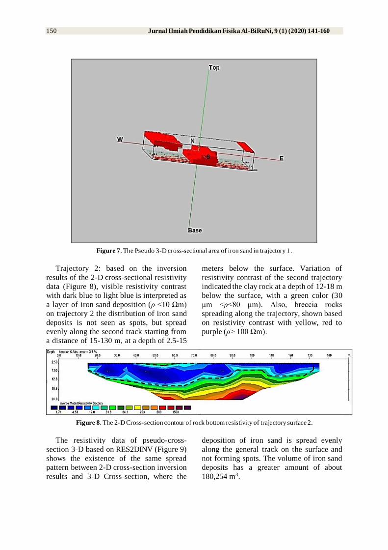
Based on RES2DINV processing data, it

can be seen that the distribution of iron sand

deposits in trajectory 1 is spread along the

research track forming sediment spots. The

processing data in the form of format (.xyz)

is reprocessed using ROCKWORK software

to find out the volume (Figure 7), it appears

that the distribution of iron sand deposits

processed by ROCKWORK has

synchronized with the results shown by

RES2DINV processing results. Based on the

calculation of the volume with a resistivity

value limit between 0-10 Ωm the volume of

iron sand trajectory 1 is 109,355 m3.


Figure 7. The Pseudo 3-D cross-sectional area of iron sand in trajectory 1.

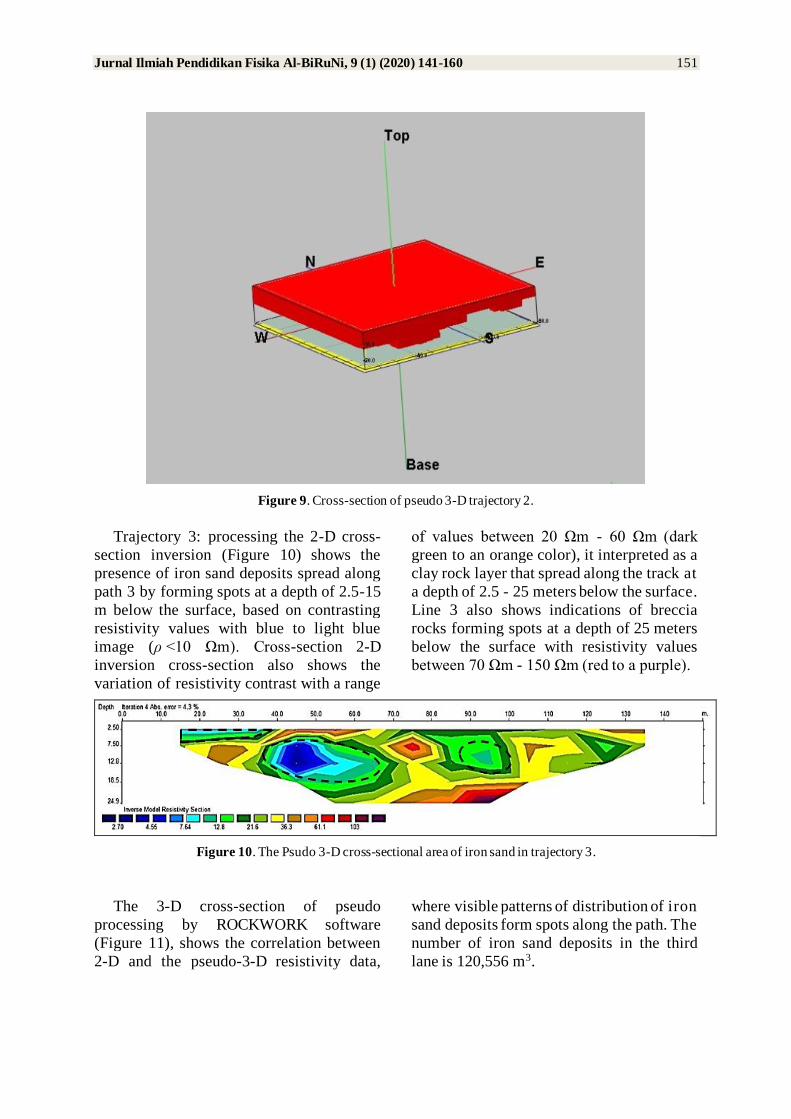
Trajectory 2: based on the inversion

results of the 2-D cross-sectional resistivity

data (Figure 8), visible resistivity contrast

with dark blue to light blue is interpreted as

a layer of iron sand deposition (ρ <10 Ωm)

on trajectory 2 the distribution of iron sand

deposits is not seen as spots, but spread

evenly along the second track starting from

a distance of 15-130 m, at a depth of 2.5-15

meters below the surface. Variation of

resistivity contrast of the second trajectory

indicated the clay rock at a depth of 12-18 m

below the surface, with a green color (30

μm <ρ<80 μm). Also, breccia rocks

spreading along the trajectory, shown based

on resistivity contrast with yellow, red to

purple (ρ> 100 Ωm).

Figure 8. The 2-D Cross-section contour of rock bottom resistivity of trajectory surface 2.

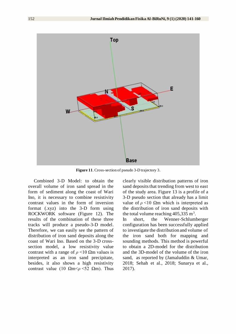
The resistivity data of pseudo-cross-

section 3-D based on RES2DINV (Figure 9)

shows the existence of the same spread

pattern between 2-D cross-section inversion

results and 3-D Cross-section, where the

deposition of iron sand is spread evenly

along the general track on the surface and

not forming spots. The volume of iron sand

deposits has a greater amount of about

180,254 m3.


Figure 9. Cross-section of pseudo 3-D trajectory 2.

Trajectory 3: processing the 2-D cross-

section inversion (Figure 10) shows the

presence of iron sand deposits spread along

path 3 by forming spots at a depth of 2.5-15

m below the surface, based on contrasting

resistivity values with blue to light blue

image (ρ <10 Ωm). Cross-section 2-D

inversion cross-section also shows the

variation of resistivity contrast with a range

of values between 20 Ωm - 60 Ωm (dark

green to an orange color), it interpreted as a

clay rock layer that spread along the track at

a depth of 2.5 - 25 meters below the surface.

Line 3 also shows indications of breccia

rocks forming spots at a depth of 25 meters

below the surface with resistivity values

between 70 Ωm - 150 Ωm (red to a purple).

Figure 10. The Psudo 3-D cross-sectional area of iron sand in trajectory 3.

The 3-D cross-section of pseudo

processing by ROCKWORK software

(Figure 11), shows the correlation between

2-D and the pseudo-3-D resistivity data,

where visible patterns of distribution of iron

sand deposits form spots along the path. The

number of iron sand deposits in the third

lane is 120,556 m3.


Figure 11. Cross-section of pseudo 3-D trajectory 3.

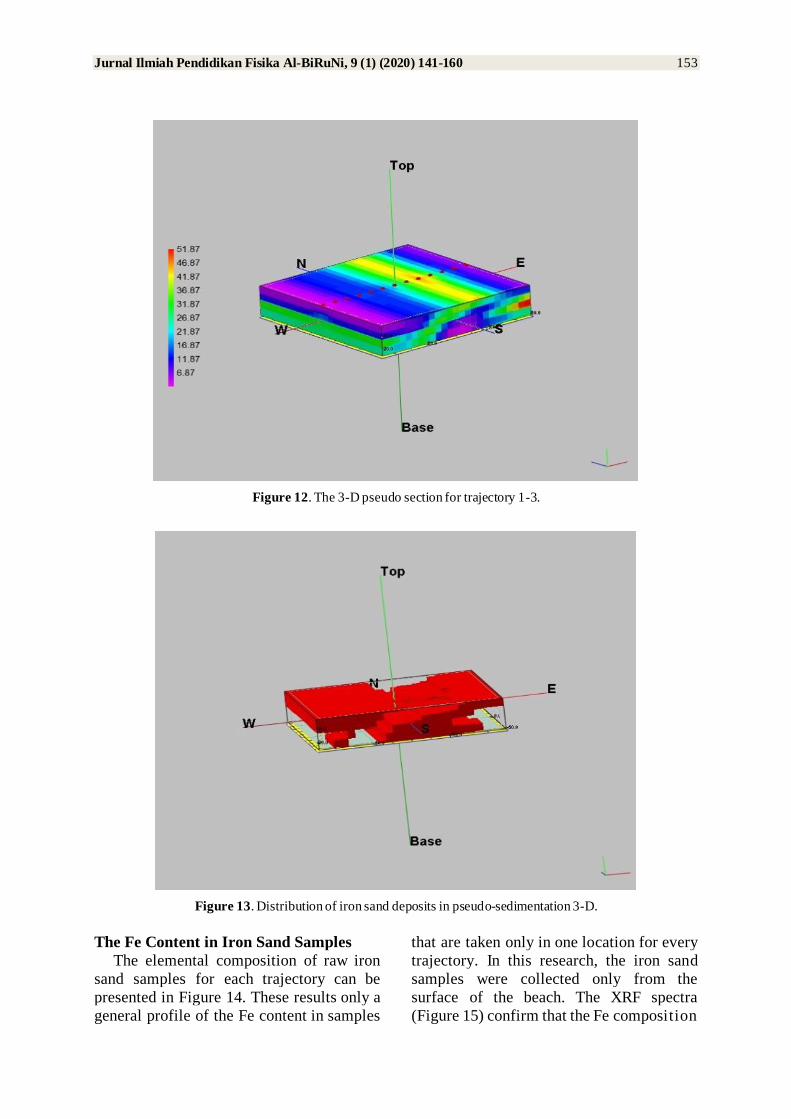
Combined 3-D Model: to obtain the

overall volume of iron sand spread in the

form of sediment along the coast of Wari

Ino, it is necessary to combine resistivity

contrast values in the form of inversion

format (.xyz) into the 3-D form using

ROCKWORK software (Figure 12). The

results of the combination of these three

tracks will produce a pseudo-3-D model.

Therefore, we can easily see the pattern of

distribution of iron sand deposits along the

coast of Wari Ino. Based on the 3-D cross-

section model, a low resistivity value

contrast with a range of ρ <10 Ωm values is

interpreted as an iron sand precipitate,

besides, it also shows a high resistivity

contrast value (10 Ωm<ρ <52 Ωm). Thus

clearly visible distribution patterns of iron

sand deposits that trending from west to east

of the study area. Figure 13 is a profile of a

3-D pseudo section that already has a limit

value of ρ <10 Ωm which is interpreted as

the distribution of iron sand deposits with

the total volume reaching 405,335 m3.

In short, the Wenner-Schlumberger

configuration has been successfully applied

to investigate the distribution and volume of

the iron sand both for mapping and

sounding methods. This method is powerful

to obtain a 2D-model for the distribution

and the 3D-model of the volume of the iron

sand, as reported by (Jamaluddin & Umar,

2018; Sehah et al., 2018; Sunarya et al.,

2017).


Figure 12. The 3-D pseudo section for trajectory 1-3.

Figure 13. Distribution of iron sand deposits in pseudo-sedimentation 3-D.

The Fe Content in Iron Sand Samples

The elemental composition of raw iron

sand samples for each trajectory can be

presented in Figure 14. These results only a

general profile of the Fe content in samples

that are taken only in one location for every

trajectory. In this research, the iron sand

samples were collected only from the

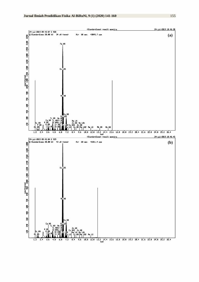
surface of the beach. The XRF spectra

(Figure 15) confirm that the Fe composition


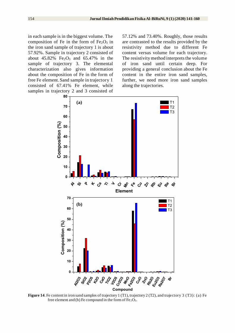
in each sample is in the biggest volume. The

composition of Fe in the form of Fe2O3 in

the iron sand sample of trajectory 1 is about

57.92%. Sample in trajectory 2 consisted of

about 45.82% Fe2O3 and 65.47% in the

sample of trajectory 3. The elemental

characterization also gives information

about the composition of Fe in the form of

free Fe element. Sand sample in trajectory 1

consisted of 67.41% Fe element, while

samples in trajectory 2 and 3 consisted of

57.12% and 73.40%. Roughly, those results

are contrasted to the results provided by the

resistivity method due to different Fe

content versus volume for each trajectory.

The resistivity method interprets the volume

of iron sand until certain deep. For

providing a general conclusion about the Fe

content in the entire iron sand samples,

further, we need more iron sand samples

along the trajectories.

Al

Si P K Ca Ti V Cr

Mn Fe

Cu

Zn

Rb

Eu

Re Br

0

10

20

30

40

50

60

70

80

Co

mp

osit

ion

(%

)

Element

T1

T2

T3

Al2

O3

SiO

2P2O

5K

2OC

aOTiO

2V2O

5C

r2O

3M

nO

Fe2

O3

CuO

ZnO

Rb2O

Eu2O

3R

e2O

7 Br

0

10

20

30

40

50

60

70

Co

mp

os

itio

n (

%)

Compound

T1

T2

T3

Figure 14. Fe content in iron sand samples of trajectory 1 (T1), trajectory 2 (T2), and trajectory 3 (T3): (a) Fe

free element and (b) Fe compound in the form of Fe2O3.

(a)

(b)


(b)

(a)


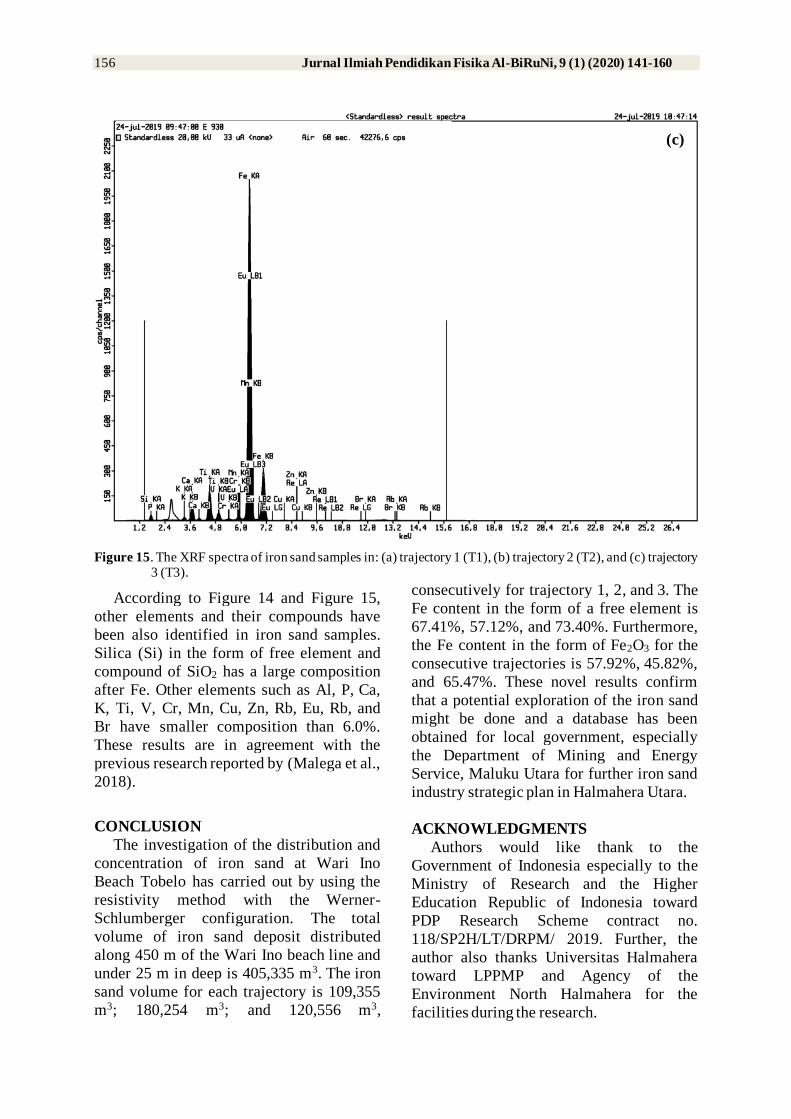
Figure 15. The XRF spectra of iron sand samples in: (a) trajectory 1 (T1), (b) trajectory 2 (T2), and (c) trajectory 3 (T3).

According to Figure 14 and Figure 15,

other elements and their compounds have

been also identified in iron sand samples.

Silica (Si) in the form of free element and

compound of SiO2 has a large composition

after Fe. Other elements such as Al, P, Ca,

K, Ti, V, Cr, Mn, Cu, Zn, Rb, Eu, Rb, and

Br have smaller composition than 6.0%.

These results are in agreement with the

previous research reported by (Malega et al.,

2018).

CONCLUSION

The investigation of the distribution and

concentration of iron sand at Wari Ino

Beach Tobelo has carried out by using the

resistivity method with the Werner-

Schlumberger configuration. The total

volume of iron sand deposit distributed

along 450 m of the Wari Ino beach line and

under 25 m in deep is 405,335 m3. The iron

sand volume for each trajectory is 109,355

m3; 180,254 m3; and 120,556 m3,

consecutively for trajectory 1, 2, and 3. The

Fe content in the form of a free element is

67.41%, 57.12%, and 73.40%. Furthermore,

the Fe content in the form of Fe2O3 for the

consecutive trajectories is 57.92%, 45.82%,

and 65.47%. These novel results confirm

that a potential exploration of the iron sand

might be done and a database has been

obtained for local government, especially

the Department of Mining and Energy

Service, Maluku Utara for further iron sand

industry strategic plan in Halmahera Utara.

ACKNOWLEDGMENTS

Authors would like thank to the

Government of Indonesia especially to the

Ministry of Research and the Higher

Education Republic of Indonesia toward

PDP Research Scheme contract no.

118/SP2H/LT/DRPM/ 2019. Further, the

author also thanks Universitas Halmahera

toward LPPMP and Agency of the

Environment North Halmahera for the

facilities during the research.

(c)


REFERENCES

Adewuyi, S. O., & Ahmed, H. A. M. (2019).

Geophysical techniques and their

applications in mining. International

Journal of Engineering Sciences &

Research Technology, 8(1).

https://doi.org/10.5281/zenodo.254988

9

Adlim, M., Khaldun, I., Rahmi, M.,

Hasanah, U., Karina, S., & Zulkiram,

Z. (2019). Determination of iron

content within iron sands from

lampanah-lengah estuary using various

analytical methods. Journal of Physics:

Conference Series, 1–8.

https://doi.org/10.1088/1755-

1315/348/1/012007

Akmam, Amir, H., Putra, A., Anshari, R., &

Jalinus, N. (2019). Implementation of

least-square constrain inversion method

of geoelectrical resistivity data wenner-

schlumberger for investigation the

characteristic of landslide. Journal of

Physics: Conference Series, 1–11.

https://doi.org/10.1088/1742-

6596/1185/1/012013

Arista, D., Rachmawati, A., Ramadhani, N.,

Saputro, R. E., Taufiq, A., &

Sunaryono. (2019). Antibacterial

performance of Fe3O4/PEG-4000

prepared by co-precipitation route.

Journal of Physics: Conference Series,

1–9. https://doi.org/10.1088/1757-

899X/515/1/012085

Arsyad, M., Tiwow, V. A., & Rampe, M. J.

(2018). Analysis of magnetic minerals

of iron sand deposit in sampulungan

beach, takalar regency, south sulawesi

using the x-ray diffraction method.


1–9. https://doi.org/10.1088/1742-

6596/1120/1/012059

Azmiyawati, C., Suyati, L., Taslimah, &

Anggraeni, R. D. (2017). Coating of

Sulfonic Silica onto Magnetite from

Coating of Sulfonic Silica onto

Magnetite from Marina Beach Iron

sand, Semarang , Indonesia. Journal of


https://doi.org/10.1088/1742-

6596/755/1/011001

Bolívar, W. M., & González, E. E. (2019).

Glutathione Fe3O4 nanoparticles as

efficient material for the adsorption of

mercury(II) from water at low

concentrations. Global Journal of

Science Frontirer Research: B, 9(1), 1–

15.

Chandra, J., & Hall, R. (2016). Tectono-

stratigrafic evolution and hydrocarbon

prospectivity of the South Halmahera

Basin, Indonesia. Proceedings of the

Indonesian Petroleum Association 27th

Annual Convention, 1–7.

Dahlan, K., Haryati, E., & Aninam, Y. S.

(2018). Potential of iron sand from

betaf beach, sarmi regency and river

sand from Doyo, Jayapura Regency,

Papua as basic materials of mortar as

nuclear radiation shielding. Journal of


https://doi.org/10.1088/1742-

6596/997/1/012023

Dang, B., Chen, Y., Wang, H., Chen, B.,

Jin, C., & Sun, Q. (2018). Preparation

of high mechanical performance Nano-

Fe3O4/Wood fiber binderless

composite boards for electromagnetic

absorption via a facile and green

method. Nanomaterials, 8(52), 1–17.

https://doi.org/10.3390/nano-8010052

Fahlepy, M. R., Tiwow, V. A., & Subaer.

(2018). Characterization of magnetite

(Fe3O4) minerals from natural iron

sand of Bonto Kanang village Takalar

for ink powder (toner) Application.

Journal of Physics: Conference Series.

https://doi.org/10.1088/1742-

6596/997/1/012036

Fahmiati, Nuryono, & Suyanta. (2017).

Characteristics of iron sand magnetic

material characteristics of iron sand

magnetic material from bugel beach,

Kulon Progo, Yogyakarta. Journal of

Physics, 1–9.

https://doi.org/10.1088/1742-

6596/755/1/011001

Haryati, E., & Dahlan, K. (2018). Potential


of iron sand from betaf beach, sarmi

regency and river sand from Doyo,

Jayapura Regency, Papua as Basic

Materials of mortar as nuclear radiation

shielding. Journal of Physics:


https://doi.org/10.1088/1742-

6596/997/1/012043

Imran, M., Ansari, A. R., Shaik, A. H.,

Abdulaziz, Hussain, S., Khan, A., &

Chandan, M. R. (2018). Ferrofluid

synthesis using oleic acid coated

Fe3O4 nanoparticles dispersed in

mineral oil for heat transfer

applications. Material Research

Express, 5(036108), 1–8.

https://doi.org/10.1088/2053-

1591/aab4d7

Jamaluddin, & Umar, E. P. (2018).

Identification of subsurface layer with

wenner- schlumberger arrays

configuration geoelectrical method.


1–7. https://doi.org/10.1088/1755-

1315/118/1/012006

Lawan, A., Raimi, J., & Ahmed, A. (2018).

Characterization of the Iron ore deposit

using 2D resistivity imaging and

induced polarization technique at

diddaye-potiskum area , Northeastern

Nigeria. Physical Science & Biophysics

Journal, 2(1), 1–12.

Malega, F., Indrayana, I. P. ., & Suharyadi,

E. (2018). Synthesis and

characterization of the microstructure

and functional group bond of fe3o4

nanoparticles from natural iron sand in

Tobelo North Halmahera. Jurnal

Ilmiah Pendidikan Fisika Al-Biruni,

7(2), 13–22. https://doi.org/10.24042/

jipfalbiruni.v7i2.2913

Maulinda, Zein, I., & Jalil, Z. (2019).

Identification of magnetite material

(Fe3O4) based on natural materials as

catalyst for industrial raw material

application. Journal of Phys, 1–7.

https://doi.org/10.1088/1742-

6596/1232/1/012054

Naveen, K. T., Rama, R. P., &

Naganjaneyulu, K. (2015). Electrical

resistivity imaging (ERI) using

multielectrodes for studying sub-

surface formations in Cauvery plains.

Advances in Applied Science Research,

6(5), 47–53.

Nurrohman, D. T., & Pribadi, J. S. (2018).

Kajian struktur kristal, lattice strain,

dan komposisi kimia nanopartikel pasir

besi yang disintesis dengan metode ball

milling. Konstan: Jurnal Fisika Dan

Pendidikan Fisika, 3(2), 47–54.

Octova, A., & Yulhendra, D. (2017). Iron

Ore deposits model using geoelectrical

resistivity method with dipole-dipole

array. MATEC Web of Conferences,

101(04017). https://doi.org/10.1051/

matecconf/201710104017

Pratiwi, E. S., Sartohadi, J., & Wahyudi.

(2019). Geoelectrical prediction for

sliding plane layers of rotational

landslide at the volcanic transitional

landscapes in Inonesia. IOP

Conference Series : Earth and

Enviromental Science.

Pratiwi, Y., Ramli, & Ratnawulan. (2017).

Pengaruh waktu milling terhadap

struktur kristal magnetite (Fe3O4)

berbahan dasar mineral vulkanik dari

gunung talang sumatera barat. Pillar of

Physics, 10, 102–108.

Raharjo, S. A., & Sehah. (2018). Eksplorasi

Potensi Pasir Besi di Pesisir Barat

Kecamatan Nusawungu Kabupaten

Cilacap Berdasarkan Data Resistivitas

Batuan Bawah Permukaan. Jurnal

Fisika Dan Aplikasinya, 14(3), 51–58.

Rahimnia, R., Salehi, Z., Ardestani, M. S.,

& Doosthoseini, H. (2019). SPION

conjugated curcumin nano-imaging

probe: Synthesis and bio-physical

evaluation. Iranian Journal of

Pharmaceutical Research, 18(1), 183–

197.

Rahmawati, R., Melati, A., Taufiq, A.,

Sunaryono, Diantoro, M., Yuliarto, B.,

Suyatman, S., Nugraha, N., &

Kurniadi, D. (2017). Preparation of

MWCNT-Fe3O4 nanocomposites from


iron sand using sonochemical route.


2–8. https://doi.org/10.1088/1757-

899X/202/1/012013

Ramelan, A. H., Wahyuningsih, S., Ismoyo,

Y. A., Pranata, H. P., & Munawaroh,

H. (2016). Preparation of xerogel SiO2

from roasted iron sand under various

acidic solution. Journal of Physics:


https://doi.org/10.1088/1742-

6596/776/1/012032

Rettob, A. L. (2019). Coating of iron sand

magnetic material with

aminobenzimidazole modified silica

via green process. Journal of Physics:


https://doi.org/10.1088/1755-

1315/235/1/012075

Rianto, D., Yulfriska, N., Murti, F.,

Hidayati, H., & Ramli, R. (2018).

Analysis of crystal structure of Fe3O4

thin films based on iron sand growth by

spin coating method. Journal of P, 1–8.

https://doi.org/10.1088/1757-

899X/335/1/012012

Sardana, N., Singh, K., Saharan, M.,

Bhatnagar, D., & Ronin, R. S. (2018).

Synthesis and characterization of

dendrimer modified magnetite

nanoparticles and their antimicrobial

activity for toxicity analysis. Journal of

Integrated Science and Technology,

6(1), 1–5.

Satriani, A., Loperte, A., Imbrenda, V., &

Lapenna, V. (2012). Geoelectrical

surveys for characterization of the

coastal saltwater intrusion in

metapontum forest reserve (Southern

Italy). International Journal of

Geophysics, 2012(238478), 1–8.

https://doi.org/10.1155/2012/238478

Sebayang, P., Kurniawan, C., Aryanto, D.,

Setiadi, E. A., Tamba, K., Djuhana, &

Sudiro, T. (2018). Preparation of

Fe3O4/ bentonite nanocomposite from

natural iron sand by co-precipitation

method for adsorbents materials.


1–8. https://doi.org/10.1088/1757-

899X/316/1/012053

Sehah, Raharjo, S. A., & Aziz, A. N. (2018).

Coastal hydrogeological model in the

iron ore prospect area of widarapayung

coastal, cilacap regency based on 2D-

resistivity data. Jurnal Penelitian

Fisika Dan Aplikasinya, 8(2), 71–83.

https://doi.org/10.26740/

jpfa.v8n2.p71-83

Sehah, Raharjo, S. A., & Destiani, F.

(2018). Interpretation of 2D-subsurface

resistivity data in the iron ore prospect

area of eastern binangun coastal,

regency of cilacap, Central Jawa.

Journal of Geoscience, Engineering,

Environment, and Technology, 3(4),

213–220.

https://doi.org/10.24273/jgeet.2018.3.4.

2139

Setiadi, E. A., Sebayang, P., Ginting, M.,

Sari, A. Y., Kurniawan, C., Saragih, C.

S., & Simamora, P. (2016). The

synthesization of Fe3O4 magnetic

nanoparticles based on natural iron

sand by co-precipitation method for the

used of the adsorption of Cu and Pb

Ions. Journal of Physics: Conference

Series, 776(012020).

https://doi.org/10.1088/ 1742-

6596/776/1/012020

Sunarya, W., Hasanuddin, Syamsudin,

Maria, & Erfan. (2017). Identifikasi

bijih besi (fe) menggunakan metoda

geolistrik resistivitas konfigurasi

werner-schlumberger di kabupaten

luwu. Jurnal Geocelebes, 1(2), 72–81.

Suprapto, S. J., & Sunuhadi, D. N. (Eds.).

(2014). Pasir besi di indonesia:

geologi, eksplorasi dan

pemanfaatannya. Pusat Sumber Daya

Geologi, Ministry of Energy and

Mineral Resources.

Taufiq, A., Saputro, R. E., Sunaryono,

Hidayat, N., Hidayat, A., Mufti, N.,

Diantoro, M., Patriati, A., Mujamilah,

Putra, E. G. R., & Nur, H. (2017).

Fabrication of magnetite nanoparticles

dispersed in olive oil and their


structural and magnetic investigations.

IOP Conference Series: Materials

Science and Engineering, 202(012008).

https://doi.org/10.1088/1757899X/202/

1/012008

The Indonesia Iron and Steel Industry

Asscociation. (2017). Indonesia steel

industry: Development &

opportunities.

Putri, W., B., K., Setiadi, E. A., Herika, V.,

Tetuko, A. P., & Sebayang, P. (2019).

Natural iron sand-based Mg 1-x

NixFe2O4 nanoparticles as potential

adsorbents for heavy metal removal

synthesized by co-precipitation

method. Journal of Physics:


https://doi.org/10.1088/1755-

1315/277/1/012031

Yulfriska, N., Rianto, D., Murti, F., Darvina,

Y., & Ramli, R. (2018). Optical

properties of Fe3O4 thin films prepared

from the iron sand by spin coating



https://doi.org/10.1088/1757-

899X/335/1/012010

Yulianto, A., Fitriawan, M., & Sumpono, I.

(2019). Synthesis of iron sand into

yellow nano-pigment using sol-gel



https://doi.org/10.1088/1742-

6596/1170/1/012049

Yusmaniar, Y., A, W. A., Hutomo, D. K., &

Handoko, E. (2018). Electromagnetic

wave absorbing properties of husk

silica-based SiO2/Fe3O4/UPR

composite. Journal of Physics:


https://doi.org/10.1088/1757-

899X/434/1/012081

Documents

Investigation of The Distribution and Fe Content of Iron