INVESTIGATION OF TECHNICAL AND OPERATIONAL INDICES FOR THE MOVEMENT OF A ROAD TRAIN

Assoc.Prof.PhD. Stoilova S, Asoc.Prof. PhD. Kunchev L, PhD. Nedelchev K. Faculty of Transport –Technical University of Sofia, Bulgaria

Abstract: In this investigation was developed method for controlling the movement of road trains on highway with minimum fuel consumption by optimizing the technical and operational parameters. To model the movement of the road train is applied graph theory. The model has been experimented for the Sofia-Plovdiv roads, as compared two parallel routes - Highway and the second category road. The model can be used to compared alternative routes for optimal management of the movement of vehicles depending on the strategy of the transport company.

Keywords: ROAD TRAINS, GRAPH THEORY, FUEL CONSUMPTION, RELATIVE PERFORMANCE, SPEED, TRANSPORT COMPANY

1. Introduction

In taking decision on the way of goods transportation, it is necessary to compare different alternatives depending on some criteria. In terms of cost reduction for transportation of the goods the main indicator is fuel consumption, which accounts for about 20% of the operating costs. Main factors in reducing fuel consumption for transport companies are: optimizing routes and load factor of vehicles. The fuel consumption depends on the following factors:

• Construction factors - type of external speed characteristics of engine, relative power, type of transmission and distribution range of gear ratios, number of gears, resistance of the tire, the air resistance. The adaptability coefficient eNMeMMk /max= can dive as better fuel economy. By increasing the relative power to a specified value, the fuel consumption per 100 km first decreases end after begins to grow Different design solutions. are applied in order to reduce fuel consumption.The aim is to reduce some natural resistance to movement of the vehicle;.

• Operational factors. The most significant impact on fuel economy is speed, type and condition of the road surface, the technical condition of the vehicle, driver qualification, and the climatic conditions. On the characteristics of fuel economy can be established that initially with increasing velocity reduces fuel consumption. After reaching minimum fuel consumption at the some speed, it began to grow up with increasing speed. The type and condition of the road surface are related to the rolling resistance of tires end loading capacity of vehicle end they influence the fuel consumption. Important in the technical condition of vehicles are: the adjustment of transmission mechanisms, mounting angles of the wheels, the air pressure in tires; adjusting in the brake mechanisms, use of appropriate fuels and lubricants, etc. Driver qualification relevant to the extra stops, which increase fuel consumption. Climatic conditions influence on rolling resistance. In snowy and wet sections, and running against the wind resistance increases by rolling, this leads to increased fuel consumption. The objective of this investigation is:

• To create and to experiment methods to determine traffic management road train on a route in which the overall fuel consumption for the individual sections of road to be minimal depending on the specified technical and operational factors.

• In case of parallel paths between the start and end point to choose the optimum.

2. Technical - operational factors dependent on fuel consumption

The main Technical - operational factors characterizing the transport process are:

• Load coefficient of the vehicle - determined based on the quantity transported in tonnes or cubic meters, relative to the maximum load of the vehicle.

• Load coefficient of the goods (load) - indicates the quantity transported in tones to the weight of the vehicle.

• Standards for fuel consumption.

Fuel saving of the vehicle depends on the design and its technical condition, modes, traffic and weather conditions, driver training, organization of the transport process and other factors.

The main Technical - Operational factors that depend on fuel are:

• Fuel consumption to travel a certain distance; • Relative performance; • Effective fuel consumption. Fuel consumption LQ to travel the distance L is determined

by:

(1) 100

.LqQ rL = ,l,

where: rq is the fuel consumption to travel 100km, l/100km; L is the length of travel distance, km.

Relative performance QW (transport operation) shows how

much cargo is transported in minimum fuel consumption and time is determined by:

(2) Lq

VmWr

Q .100..

= , t/lh,

where: m is the total mass of vehicle and cargo,t. V is motion speed, km/h.

Efficient fuel consumption eq characterized by the capacity of the vehicle to perform work with minimum fuel consumption and time:

(3) 100...1

VmLq

Wq r

Qe == , l.h/tkm.

Main factors in choosing a route between two points are :distance (km), limit of delivery (travel time, h), fuel consumption (l/km). Delivery time depends on the duration of loading and unloading operations at the initial and final destination and the duration of travel time. Since loading and unloading operations do not influence fuel economy, they will not be take account in the paper. The duration of the road train movement in different areas depends on road conditions - Plan and profile of road radius curves, limit the maximum speed, road conditions, weather conditions, vehicle load, etc. Travel time can be defined in terms of minimum fuel consumption and maximum speed.

3. Methods for analytical determination of road fuel consumption of vehicle

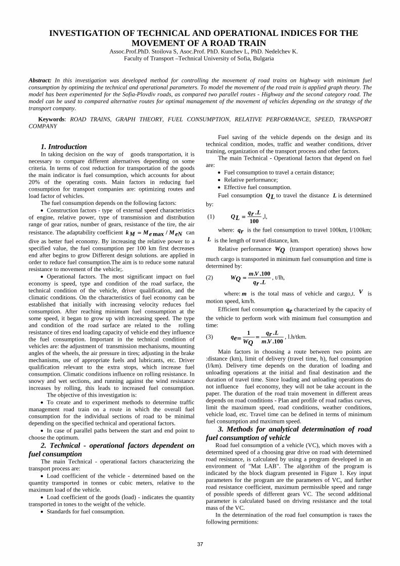
Road fuel consumption of a vehicle (VC), which moves with a determined speed of a choosing gear drive on road with determined road resistance, is calculated by using a program developed in an environment of "Mat LAB". The algorithm of the program is indicated by the block diagram presented in Figure 1. Key input parameters for the program are the parameters of VC, and further road resistance coefficient, maximum permissible speed and range of possible speeds of different gears VC. The second additional parameter is calculated based on driving resistance and the total mass of the VC.

In the determination of the road fuel consumption is такеs the following permitions:

37

• In each section VC is moving uniformly with constant speed;

• Changing the specific fuel consumption at different engine load is determined by the polynomial of second degree according to [3];

• Do not take acount of the action of a counterclaim or tailwind on the fuel consumption of VC;

• Do not take account of the movement options of VC by inertia(with gear on or off);

• Do not take account for the impact of domestic consumers on the VC change rate of load. The fuel l/100km in VC is determined as:

(4) ( )ifwtf

peikr PPP

v

Kgq ±+=

...36

., ηρ

, l/100km,

Where: ge = f(ne) is the specific fuel consumption at maximum load;

Kр – coefficient of the load, determine the formula (2) according to [3];

Ap = 1,7; Bp = 2,63 and Cp = 1,93 – coefficients of polynomial (5) determining engine load;

ρf = 0,86 g/dm3 – fuel specific density; ηt – efficiency of the transmission, ηt = 0,92; v – speed of the VC, m/s; Pw – power needed to overcome the force of air resistance

acting on the VC, kW; Pf – power needed to overcome the resistance of the rolling

effect in the VC, kW; Pi – power needed to overcome the force resistance from the

slope acting on the road to VC, kW;

(6) 2.. pppppp CBAK χχ +−=

(7) k

ifwkcp P

PPP

PP ±+

==χ ,

where: Pc – general resistance power, kW; cx – resistant coefficient from the air.

(8) tek

PP

η= , kW

(9) 33 10.....5,0 −= vScP airxw ρ , kW

(10) 320 10..81,9... −

+= vmvkfP jff , kW

(11) 310..81,9.. −= vmiP jri , kW

Here ρair is the air density, kg/m3; S = 0,9.H1.B2 – frontal area of the VC, m; f0 – basic coefficient of rolling resistance; kf – coefficient taking into account the increase of the

coefficient of rolling resistance with increasing speed, s2/m2; mj – mass, kg (mj = mL = 18000 kg; mj = mU = 8000 kg ); ir = Δhi/Li – road resistance coefficient of the road section; Δhi = hi+1 – hi – difference in altitude between the end and

beginning of the road section, m; Li – length of road section, m; hi – altitude at the beginning of the road section, m; hi+1 – altitude at the beginning of the road section, m

(12) kke r

viin

....30 0

π= , 1/min

(13) k

kei ii

rnv

k ..30

..

0min,

min,π

= , m/s

(14) k

kei ii

rnv

k ..30

..

0max,

max,π

= , m/s,

where: vmin,ik – minimum possible speed on the ik-тата gear m/s;

vmax,ik – maximum possible speed on the ik-тата gear, m/s;

vmax,c – the maximum possible speed of movement of VC, m/s (determined from Equation 14);

vmax,L – maximum permitted speed for the road section, km/h (fig.3);

vmin,b – minimum speed that determines the fuel consumption of road section, km/h (fig.4);

vmax,b – maximum permitted speed for the road section, km/h (fig.4);

Lir – lenght of road, km; ne – angular speed of the engine, 1/min; i0 – the main transmission ratio; ik – the transmission ratio of gearbox, which moves VC; rk – kinematic wheel radius, m;

Fig.1. Block diagram of algorithm for calculation of road fuel to vehicle

(15) max,max,2max,0

3max,

.81.9...

....5,0

kcjrcf

cairx

Pvmivkf

vSc

=

±++

+ρ

Fuel consumption Qc,ir for passage of road section length Lir, is determined by

(16) irikr

ic Lq

Qk

.100

,, = , l

Relative performance WQ,ik , tkm/(hL) of road section length Lir,

is determined by

(17) 10..

..6,3

1000.

..6,3

,,,

irikrj

icj

iQ Lq

vm

Q

vmW

kk

== , t.km/(h.L)

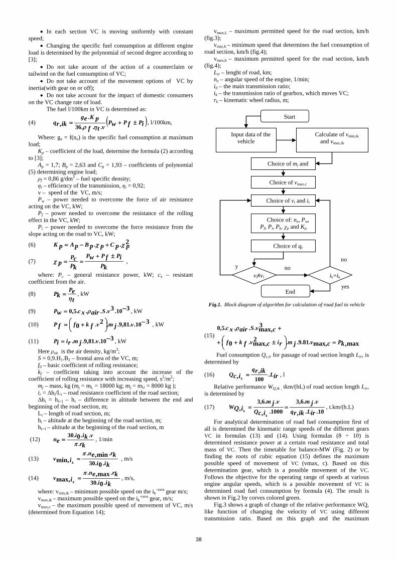
For analytical determination of road fuel consumption first of all is determined the kinematic range speeds of the different gears VC in formulas (13) and (14). Using formulas (8 ÷ 10) is determined resistance power at a certain road resistance and total mass of VC. Then the timetable for balance-MW (Fig. 2) or by finding the roots of cubic equation (15) defines the maximum possible speed of movement of VC (vmax, c). Based on this determination gear, which is a possible movement of the VC. Follows the objective for the operating range of speeds at various engine angular speeds, which is a possible movement of VC is determined road fuel consumption by formula (4). The result is shown in Fig.2 by corves colored green.

Fig.3 shows a graph of change of the relative performance WQ, like function of changing the velocity of VC using different transmission ratio. Based on this graph and the maximum

End

Choice of qr

Start

Input data of the vehicle

Calculate of vmin,ik and vmax,ik

Choice of mj and

Choice of vmax,c

Choice of vi and ir

Choice of: ne, Pw,

Pf, Pi, Pk, χp and Kp

vi#vi

ik=ik

y

no

yes

no

38

authorized speed of a road section is defined range of recommended speeds of the VC and possible transmission ratio (wich is a possible motion) In the recommended range of speeds from Fig.3 (green curves for travel expenses) or formula (4 ÷ 12) is defined road fuel consumption of a gear transmission ratio driving the VC with a speed necessary for the implementation of procedures. optimization

Fig.2. Balance - MW

Fig. 3. Amendment of optimization parameters change the speed of the

different gears at a certain road resistance ir.

Fig. 4. Amendment of the maximum possible speed (vmax, c)

modification of the TC in the driving resistance

4. Method for simulation the road train service at optimal consumption on fuell

4.1. Basic principle The theory of optimal control is associated with the

establishment of such values of control parameters ix , ni ,...,1= , to ensure that maximum, or minimum of set target function: (18) ),...,...,,( 21 ni xxxxfZ = max (min)

in the following restrictive conditions:

(19)

mnm

nn

bxxx

bxxxbxxx

≤

≤

≤

),...,,(...

),...,,(),...,,(

21

22121211

ϕ

ϕϕ

, mj ,...,1= , ni ,...,1= ,

0,...,, 21 ≥nxxx . That said optimization model is characterized by the type of

objective function, the type of restrictive conditions and required parameters to be integers. The target function can be linear or a nonlinear, restrictive condition itself also may be linear or nonlinear. Depending on these characteristics are selected the optimization methods.

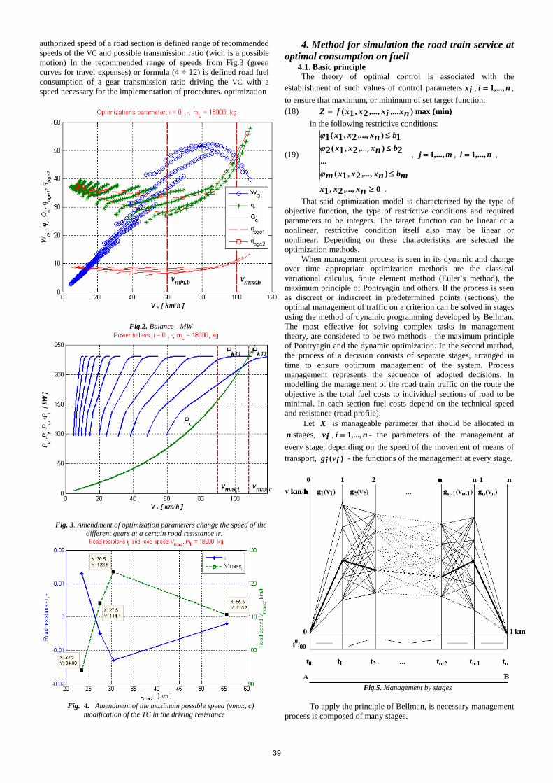
When management process is seen in its dynamic and change over time appropriate optimization methods are the classical variational calculus, finite element method (Euler’s method), the maximum principle of Pontryagin and others. If the process is seen as discreet or indiscreet in predetermined points (sections), the optimal management of traffic on a criterion can be solved in stages using the method of dynamic programming developed by Bellman. The most effective for solving complex tasks in management theory, are considered to be two methods - the maximum principle of Pontryagin and the dynamic optimization. In the second method, the process of a decision consists of separate stages, arranged in time to ensure optimum management of the system. Process management represents the sequence of adopted decisions. In modelling the management of the road train traffic on the route the objective is the total fuel costs to individual sections of road to be minimal. In each section fuel costs depend on the technical speed and resistance (road profile).

Let X is manageable parameter that should be allocated in n stages, iv , ni ,...,1= - the parameters of the management at every stage, depending on the speed of the movement of means of transport, )( ii vg - the functions of the management at every stage.

Fig.5. Management by stages

To apply the principle of Bellman, is necessary management

process is composed of many stages.

39

This happens at every stage i determines the optimum value of the variable iv and function )( ii vg , fig.5. Solving the task is done by recursive equations.

(20)

)}(min{)()}()(min{)(

...)}()(min{)(

...)}()(min{)(

11121222

1

1

vgXfvXfvgXf

vXfvgXf

vXfvgXf

kkkkk

nnnnn

=−+=

−+=

−+=

−

−

Solving the equations is done in the opposite direction, by the

construction a function )(1 Xf , then determined )(2 Xf so the

definition of )(Xfn , which is the solution of the problem. At every stage of solving the problem is determined values

nvvv ,..,, 21 , which has received the optimal solution 4.2. Mathematical model The principle of separation of decision stages, which is the

main method of dynamic optimization is used to develop a methodology for modeling the movement of a road train on the route with selected criterion.

The movement of the road train is presented as a network formed by sections of the route and variants of management in each area. For this purpose:

• The route of movement of the road train is divided into separate sections according to the profile of the path. For each section are determined:

o maximum speed; o potential traffic speeds in different gears; • Choice of optimization criterion. • It is necessary to determine traffic management of the

road train on the route for which summary fuel costs to individual sections of road to be minimal. In each section of road fuel costs depend on the technical speed and resistance movement (road profile).

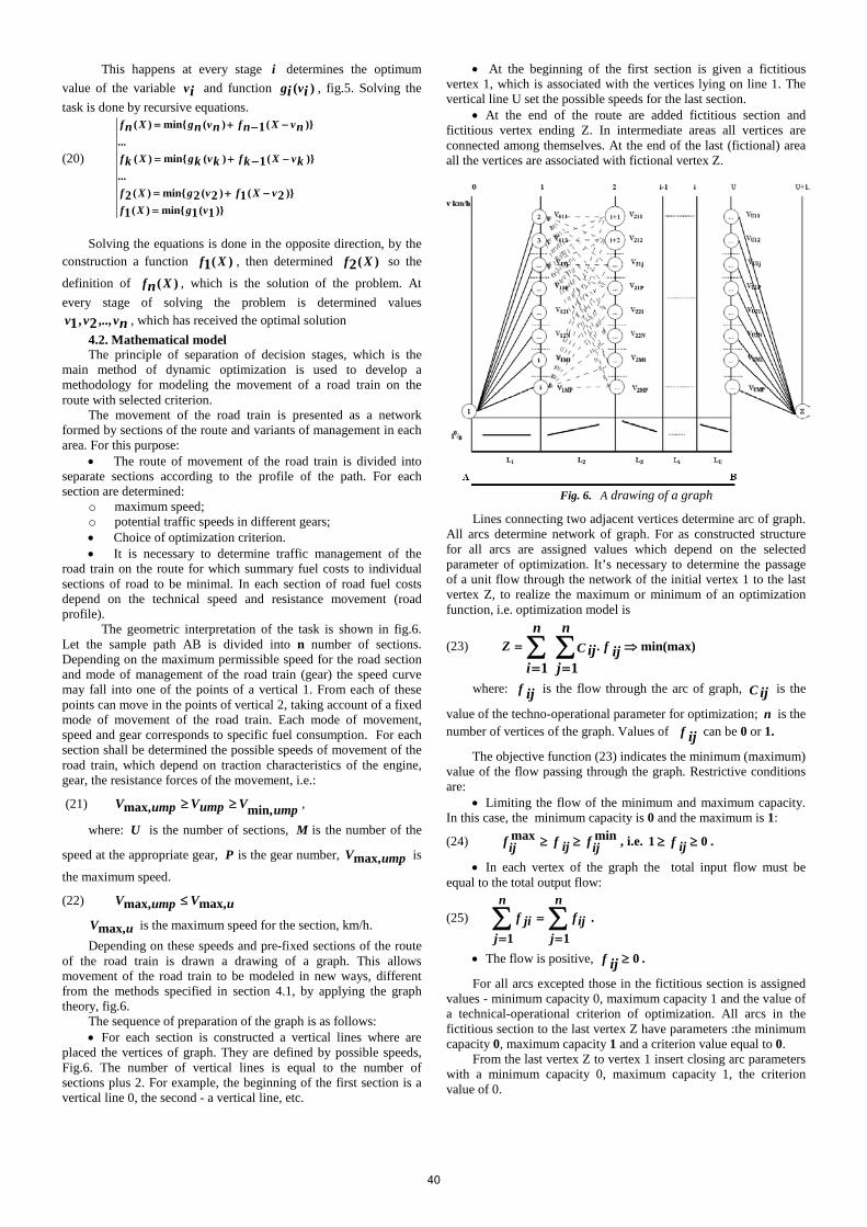
The geometric interpretation of the task is shown in fig.6. Let the sample path AB is divided into n number of sections. Depending on the maximum permissible speed for the road section and mode of management of the road train (gear) the speed curve may fall into one of the points of a vertical 1. From each of these points can move in the points of vertical 2, taking account of a fixed mode of movement of the road train. Each mode of movement, speed and gear corresponds to specific fuel consumption. For each section shall be determined the possible speeds of movement of the road train, which depend on traction characteristics of the engine, gear, the resistance forces of the movement, i.e.:

(21) umpVumpVumpV min,max, ≥≥ ,

where: U is the number of sections, M is the number of the

speed at the appropriate gear, P is the gear number, umpVmax, is

the maximum speed.

(22) uVumpV max,max, ≤

uVmax, is the maximum speed for the section, km/h. Depending on these speeds and pre-fixed sections of the route

of the road train is drawn a drawing of a graph. This allows movement of the road train to be modeled in new ways, different from the methods specified in section 4.1, by applying the graph theory, fig.6.

The sequence of preparation of the graph is as follows: • For each section is constructed a vertical lines where are

placed the vertices of graph. They are defined by possible speeds, Fig.6. The number of vertical lines is equal to the number of sections plus 2. For example, the beginning of the first section is a vertical line 0, the second - a vertical line, etc.

• At the beginning of the first section is given a fictitious vertex 1, which is associated with the vertices lying on line 1. The vertical line U set the possible speeds for the last section.

• At the end of the route are added fictitious section and fictitious vertex ending Z. In intermediate areas all vertices are connected among themselves. At the end of the last (fictional) area all the vertices are associated with fictional vertex Z.

Fig. 6. A drawing of a graph

Lines connecting two adjacent vertices determine arc of graph. All arcs determine network of graph. For as constructed structure for all arcs are assigned values which depend on the selected parameter of optimization. It’s necessary to determine the passage of a unit flow through the network of the initial vertex 1 to the last vertex Z, to realize the maximum or minimum of an optimization function, i.e. optimization model is

(23) min(max).

11⇒= ∑∑

==fCZ ij

n

jij

n

i

where: f ij is the flow through the arc of graph, C ij is the

value of the techno-operational parameter for optimization; n is the number of vertices of the graph. Values of f ij can be 0 or 1.

The objective function (23) indicates the minimum (maximum) value of the flow passing through the graph. Restrictive conditions are:

• Limiting the flow of the minimum and maximum capacity. In this case, the minimum capacity is 0 and the maximum is 1:

(24) minmaxijff ijijf ≥≥ , i.e. 01 ≥≥ f ij .

• In each vertex of the graph the total input flow must be equal to the total output flow:

(25) ∑∑=

=

=

n

jijf

n

jjif

11.

• The flow is positive, 0≥f ij .

For all arcs excepted those in the fictitious section is assigned values - minimum capacity 0, maximum capacity 1 and the value of a technical-operational criterion of optimization. All arcs in the fictitious section to the last vertex Z have parameters :the minimum capacity 0, maximum capacity 1 and a criterion value equal to 0. From the last vertex Z to vertex 1 insert closing arc parameters with a minimum capacity 0, maximum capacity 1, the criterion value of 0.

40

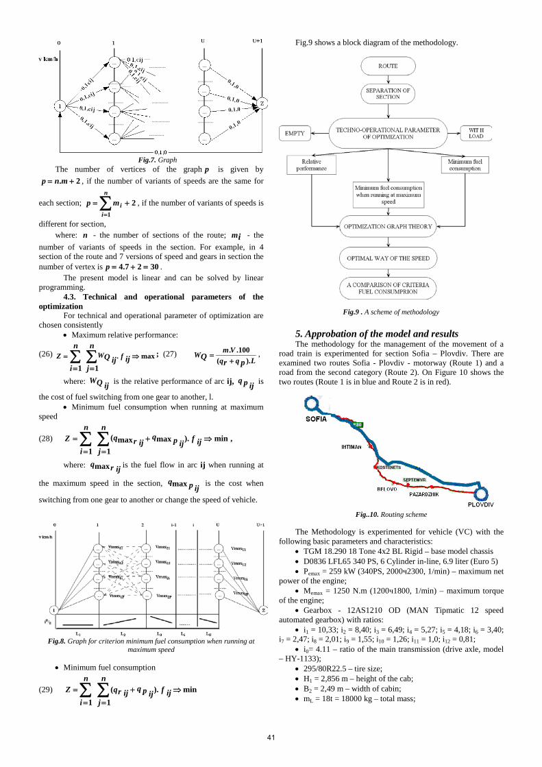
Fig.7. Graph

The number of vertices of the graph p is given by 2. += mnp , if the number of variants of speeds are the same for

each section; 21

+=∑=

n

iimp , if the number of variants of speeds is

different for section, where: n - the number of sections of the route; im - the number of variants of speeds in the section. For example, in 4 section of the route and 7 versions of speed and gears in section the number of vertex is 3027.4 =+=p .

The present model is linear and can be solved by linear programming.

4.3. Technical and operational parameters of the optimization

For technical and operational parameter of optimization are chosen consistently

• Maximum relative performance:

(26) max.

11⇒= ∑∑

==fWZ ij

n

jQ ij

n

i

; (27) Lqq

VmWpr

Q ).(100..

+= ,

where: QW ij is the relative performance of arc ij, pq ij is

the cost of fuel switching from one gear to another, l. • Minimum fuel consumption when running at maximum

speed

(28) min).max1

max(

1⇒+

==

= ∑∑ f ijpqij

n

jrq ij

n

iZ ,

where: rq ijmax is the fuel flow in arc ij when running at

the maximum speed in the section, pqijmax is the cost when

switching from one gear to another or change the speed of vehicle.

Fig.8. Graph for criterion minimum fuel consumption when running at

maximum speed

• Minimum fuel consumption

(29) min).1(

1⇒+

==

= ∑∑ f ijpq ij

n

jrq ij

n

iZ

Fig.9 shows a block diagram of the methodology.

Fig.9 . A scheme of methodology 5. Approbation of the model and results The methodology for the management of the movement of a road train is experimented for section Sofia – Plovdiv. There are examined two routes Sofia - Plovdiv - motorway (Route 1) and a road from the second category (Route 2). On Figure 10 shows the two routes (Route 1 is in blue and Route 2 is in red).

Fig..10. Routing scheme

The Methodology is experimented for vehicle (VC) with the following basic parameters and characteristics:

• TGM 18.290 18 Tone 4x2 BL Rigid – base model chassis • D0836 LFL65 340 PS, 6 Cylinder in-line, 6.9 liter (Euro 5) • Pemax = 259 kW (340PS, 2000ч2300, 1/min) – maximum net

power of the engine; • Memax = 1250 N.m (1200ч1800, 1/min) – maximum torque

of the engine; • Gearbox - 12AS1210 OD (MAN Tipmatic 12 speed

automated gearbox) with ratios: • i1 = 10,33; i2 = 8,40; i3 = 6,49; i4 = 5,27; i5 = 4,18; i6 = 3,40;

i7 = 2,47; i8 = 2,01; i9 = 1,55; i10 = 1,26; i11 = 1,0; i12 = 0,81; • i0= 4.11 – ratio of the main transmission (drive axle, model

– HY-1133); • 295/80R22.5 – tire size; • H1 = 2,856 m – height of the cab; • B2 = 2,49 m – width of cabin; • mL = 18t = 18000 kg – total mass;

41

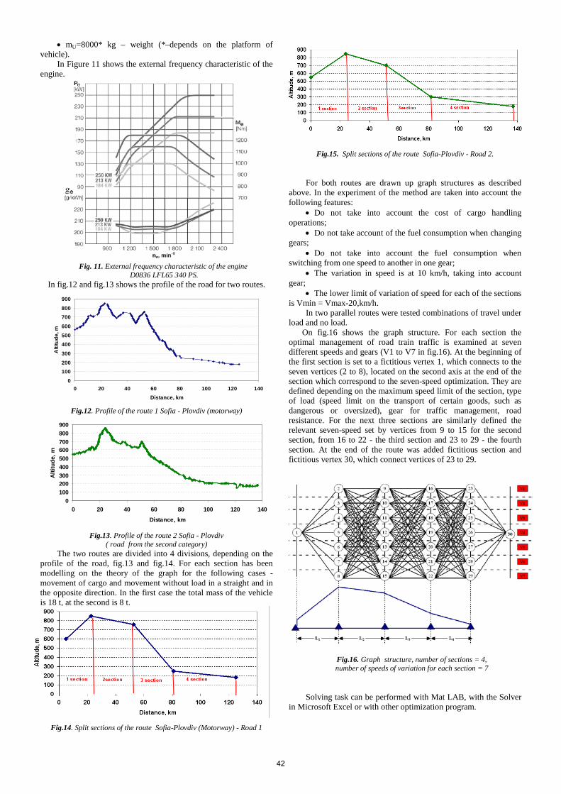
• mU=8000* kg – weight (*–depends on the platform of vehicle). In Figure 11 shows the external frequency characteristic of the engine.

Fig. 11. External frequency characteristic of the engine

D0836 LFL65 340 PS. In fig.12 and fig.13 shows the profile of the road for two routes.

0100200300400500600700800900

0 20 40 60 80 100 120 140Distance, km

Alti

tude

, m

Fig.12. Profile of the route 1 Sofia - Plovdiv (motorway)

0100200300400500600700800900

0 20 40 60 80 100 120 140

Distance, km

Altit

ude,

m

Fig.13. Profile of the route 2 Sofia - Plovdiv

( road from the second category) The two routes are divided into 4 divisions, depending on the

profile of the road, fig.13 and fig.14. For each section has been modelling on the theory of the graph for the following cases - movement of cargo and movement without load in a straight and in the opposite direction. In the first case the total mass of the vehicle is 18 t, at the second is 8 t.

Fig.14. Split sections of the route Sofia-Plovdiv (Motorway) - Road 1

Fig.15. Split sections of the route Sofia-Plovdiv - Road 2. For both routes are drawn up graph structures as described

above. In the experiment of the method are taken into account the following features:

• Do not take into account the cost of cargo handling operations;

• Do not take account of the fuel consumption when changing gears;

• Do not take into account the fuel consumption when switching from one speed to another in one gear;

• The variation in speed is at 10 km/h, taking into account gear;

• The lower limit of variation of speed for each of the sections is Vmin = Vmax-20,km/h. In two parallel routes were tested combinations of travel under load and no load.

On fig.16 shows the graph structure. For each section the optimal management of road train traffic is examined at seven different speeds and gears (V1 to V7 in fig.16). At the beginning of the first section is set to a fictitious vertex 1, which connects to the seven vertices (2 to 8), located on the second axis at the end of the section which correspond to the seven-speed optimization. They are defined depending on the maximum speed limit of the section, type of load (speed limit on the transport of certain goods, such as dangerous or oversized), gear for traffic management, road resistance. For the next three sections are similarly defined the relevant seven-speed set by vertices from 9 to 15 for the second section, from 16 to 22 - the third section and 23 to 29 - the fourth section. At the end of the route was added fictitious section and fictitious vertex 30, which connect vertices of 23 to 29.

Fig.16. Graph structure, number of sections = 4, number of speeds of variation for each section = 7

Solving task can be performed with Mat LAB, with the Solver in Microsoft Excel or with other optimization program.

42

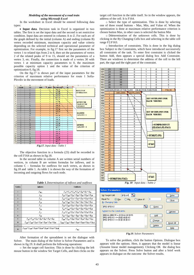
Modeling of the movement of a road train using Microsoft Excel

In the worksheet in Excel should be entered following data types:

• Input data. Decision task in Excel is organized in two tables. The first is set the input data and the second is set restrictive condition. Input data are entered in columns A to Z. For each arc of the graph defined by the initial (column A) and ending (column B) vertex recorded minimum, maximum capacity and value criteria depending on the selected technical and operational parameter of optimization. For example, in fig.17 first set the parameters of the vertex 1 to related tips from 2 to 8, then set the parameters of vertex 2 of the related peaks of 9 to 15, should set the parameters of a vertex 3, etc. Finally, the connection is made of a vertex 30 with vertex 1 at minimum capacity parameters to 0, the maximum possible capacity option 1 and the value of the criterion of optimization 0, fig.18. On the fig.17 is shown part of the input parameters for the criterion of maximum relative performance for route 1 Sofia-Plovdiv in the movement of loads.

Fig.17. Input data - Table 1

The objective function in a formula (23) shall be recorded in the cell F164 as shown in fig.18. In the second table in column A are written serial numbers of vertices, in column B are written formulas for inflows, and in column C – formulas for outflows for each vertex, as shown in fig.18 and table 1. As table 1 is shown the way of the formation of incoming and outgoing flows for each node. Table 1.Determination of inflows and outflows

After formation of the spreadsheet is set the dialogue with Solver. The main dialog of the Solver is Solver Parameters and is shown in fig.19. It shall perform the following operations:

o Set the target cell function. This is done by clicking the left mouse button in the window Set Target Cells, and then clicks on the

target cell function in the table itself. So in the window appears, the address of the cell. It is F164.

o Select the type of optimization. This is done by selecting one of three round buttons - Max, Min, and Value of. When the optimization is done at maximum relative performance criterion is chosen button Max, in other cases is selected the button Min

o Ddetermination of the unknown cells. This is done by clicking in the By Changing Cells box and selecting in the table cell range F2:F163.

o Introduction of constraints. This is done in the big dialog box Subject to the Constraints, which have introduced successively all constraints of the task. To enter first constraint is clicked the button Add, then appears a special dialog box Add Constraint. There are windows to determine the address of the cell to the left part, the sign and the right part of the constraint.

Fig. 18 Input data - Table 2

Fig.19. Solver Parameters

To solve the problem, click the button Options. Dialogue box appears with the options. Here, it appears that the model is linear (Assume linear model management). Clicking OK the dialog box appears on the Solver. Press Solve button and after a brief work appears in dialogue on the outcome the Solver results.

43

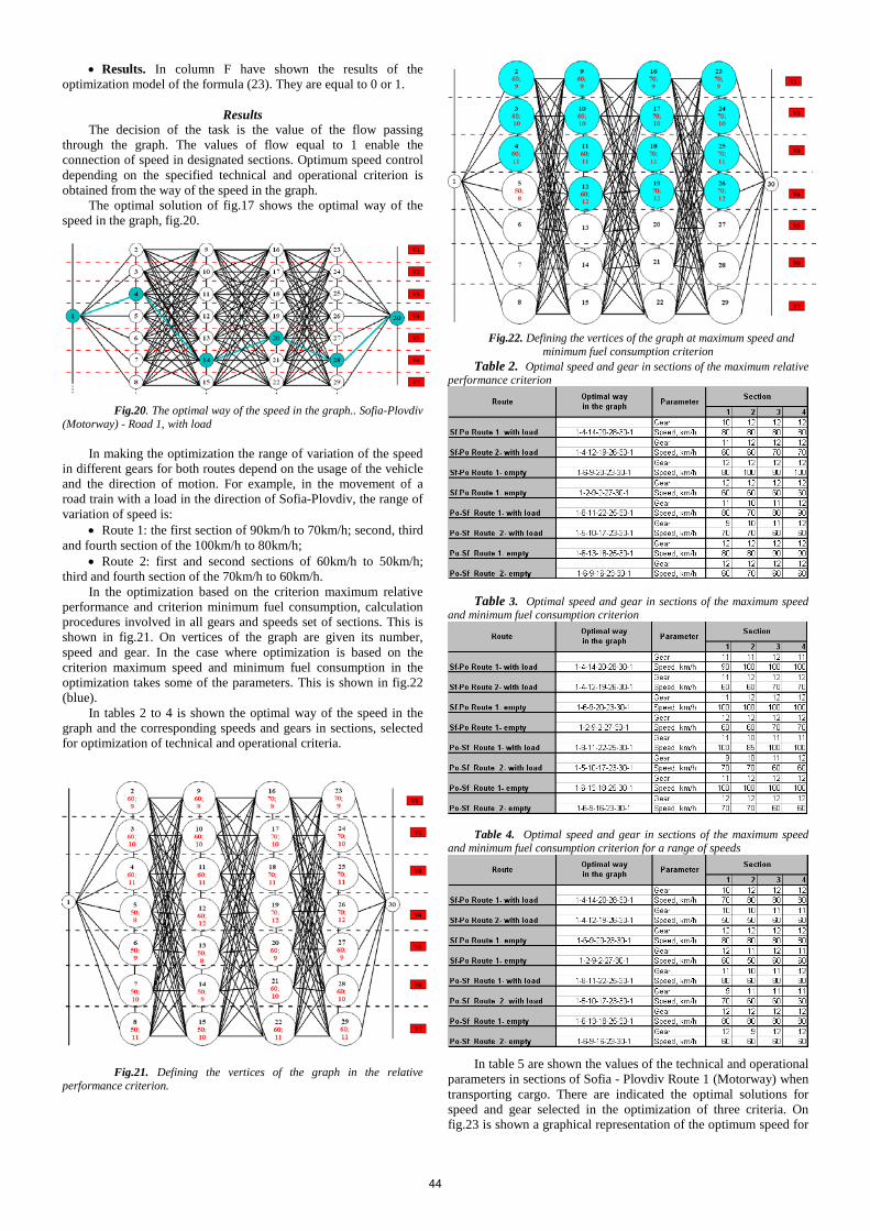
• Results. In column F have shown the results of the optimization model of the formula (23). They are equal to 0 or 1.

Results

The decision of the task is the value of the flow passing through the graph. The values of flow equal to 1 enable the connection of speed in designated sections. Optimum speed control depending on the specified technical and operational criterion is obtained from the way of the speed in the graph.

The optimal solution of fig.17 shows the optimal way of the speed in the graph, fig.20.

Fig.20. The optimal way of the speed in the graph.. Sofia-Plovdiv

(Motorway) - Road 1, with load In making the optimization the range of variation of the speed

in different gears for both routes depend on the usage of the vehicle and the direction of motion. For example, in the movement of a road train with a load in the direction of Sofia-Plovdiv, the range of variation of speed is:

• Route 1: the first section of 90km/h to 70km/h; second, third and fourth section of the 100km/h to 80km/h;

• Route 2: first and second sections of 60km/h to 50km/h; third and fourth section of the 70km/h to 60km/h. In the optimization based on the criterion maximum relative performance and criterion minimum fuel consumption, calculation procedures involved in all gears and speeds set of sections. This is shown in fig.21. On vertices of the graph are given its number, speed and gear. In the case where optimization is based on the criterion maximum speed and minimum fuel consumption in the optimization takes some of the parameters. This is shown in fig.22 (blue).

In tables 2 to 4 is shown the optimal way of the speed in the graph and the corresponding speeds and gears in sections, selected for optimization of technical and operational criteria.

Fig.21. Defining the vertices of the graph in the relative

performance criterion.

Fig.22. Defining the vertices of the graph at maximum speed and

minimum fuel consumption criterion Table 2. Optimal speed and gear in sections of the maximum relative

performance criterion

Table 3. Optimal speed and gear in sections of the maximum speed and minimum fuel consumption criterion

Table 4. Optimal speed and gear in sections of the maximum speed and minimum fuel consumption criterion for a range of speeds

In table 5 are shown the values of the technical and operational

parameters in sections of Sofia - Plovdiv Route 1 (Motorway) when transporting cargo. There are indicated the optimal solutions for speed and gear selected in the optimization of three criteria. On fig.23 is shown a graphical representation of the optimum speed for

44

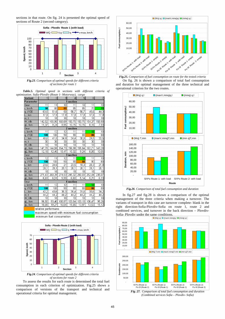
sections in that route. On fig. 24 is presented the optimal speed of sections of Route 2 (second category).

Sofia - Plovdiv Route 1 (with load)

0102030405060708090

100

1 2 3 4Section

Spee

d, k

m/h

WQ V,q q v max, km/h

Fig.23. Comparison of optimal speeds for different criteria

of sections for route 1 Table.5. Optimal speed in sections with different criteria of

optimization. Sofia-Plovdiv (Route 1- Motorway), cargo

Sofia - Plovdiv Route 2 (with load)

0

10

20

30

40

50

60

70

1 2 3 4Section

Spee

d, k

m/h

WQ V,q q v max, km/h

Fig.24. Comparison of optimal speeds for different criteria

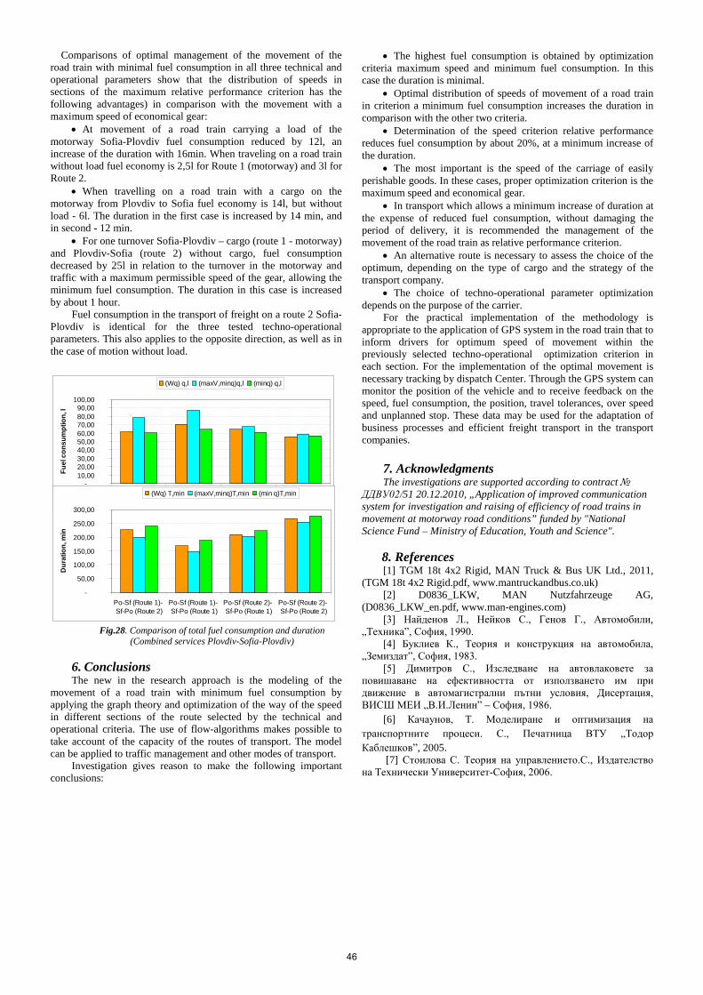
of sections for route 2 To assess the results for each route is determined the total fuel consumption in each criterion of optimization. Fig.25 shows a comparison of versions of the transport and technical and operational criteria for optimal management.

-

10,00

20,00

30,00

40,00

50,00

60,00

Sf-Po Route

1- with

load

Sf-Po Route

2- with

load

Sf-Po Route

1- em

pty

Sf-Po Route

2- em

pty

Po-Sf R

oute 1-

with lo

ad

Po-Sf R

oute 2

- with

load

Po-Sf R

oute 1-

empty

Po-Sf R

oute 2

- empty

Fuel

con

sum

ptio

n, l

(Wq) q,l (maxV,minq)q,l (minq) q,l

Fig.25. Comparison of fuel consumption on route for the tested criteria

On fig. 26 is shown a comparison of total fuel consumption and duration for optimal management of the three technical and operational criterion for the two routes.

Fig.26. Comparison of total fuel consumption and duration

In fig.27 and fig.28 is shown a comparison of the optimal management of the three criteria when making a turnover. The variants of transport in this case are turnover complete- blank in the right direction-Sofia-Plovdiv-Sofia on route 1, route 2 and combined services, and turnover in the back direction – Plovdiv- Sofia- Plovdiv under the same conditions.

Fig. 27. Comparison of total fuel consumption and duration (Combined services Sofia – Plovdiv- Sofia)

-

10,00

20,00

30,00

40,00

50,00

60,00

Sf-Po Route 1- with load Sf-Po Route 2- with load

Маршрут

Fuel

con

sum

ptio

n,l

(Wq) q,l (maxV,minq)q,l (minq) q,l

- 20,00 40,00 60,00 80,00

100,00 120,00 140,00 160,00

Sf-Po Route 1- with load Sf-Po Route 2- with load

Route

Dura

tion,

min

(Wq) T,min (maxV,minq)T,min (min q)T,min

- 10,00 20,00 30,00 40,00 50,00 60,00 70,00 80,00 90,00

Sf-Po (Route 1)- Po-Sf (Route 2)

Sf-Po (Route 1)- Po-Sf (Route 1)

Sf-Po (Route 2)- Po-Sf (Route 1)

Sf-Po (Route 2)- Po-Sf (Route 2)

Маршрути

Fuel

con

sum

ptio

n, l

(Wq) q,l (maxV,minq)q,l (minq) q,l

-

50,00

100,00

150,00

200,00

250,00

300,00

Sf-Po (Route 1)- Po-Sf (Route 2)

Sf-Po (Route 1)- Po-Sf (Route 1)

Sf-Po (Route 2)- Po-Sf (Route 1)

Sf-Po (Route 2)- Po-Sf (Route 2)

Dur

atio

n,m

in

(Wq) T,min (maxV,minq)T,min (min q)T,min

45

Comparisons of optimal management of the movement of the road train with minimal fuel consumption in all three technical and operational parameters show that the distribution of speeds in sections of the maximum relative performance criterion has the following advantages) in comparison with the movement with a maximum speed of economical gear:

• At movement of a road train carrying a load of the motorway Sofia-Plovdiv fuel consumption reduced by 12l, an increase of the duration with 16min. When traveling on a road train without load fuel economy is 2,5l for Route 1 (motorway) and 3l for Route 2.

• When travelling on a road train with a cargo on the motorway from Plovdiv to Sofia fuel economy is 14l, but without load - 6l. The duration in the first case is increased by 14 min, and in second - 12 min.

• For one turnover Sofia-Plovdiv – cargo (route 1 - motorway) and Plovdiv-Sofia (route 2) without cargo, fuel consumption decreased by 25l in relation to the turnover in the motorway and traffic with a maximum permissible speed of the gear, allowing the minimum fuel consumption. The duration in this case is increased by about 1 hour. Fuel consumption in the transport of freight on a route 2 Sofia-Plovdiv is identical for the three tested techno-operational parameters. This also applies to the opposite direction, as well as in the case of motion without load.

Fig.28. Comparison of total fuel consumption and duration (Combined services Plovdiv-Sofia-Plovdiv)

6. Conclusions The new in the research approach is the modeling of the movement of a road train with minimum fuel consumption by applying the graph theory and optimization of the way of the speed in different sections of the route selected by the technical and operational criteria. The use of flow-algorithms makes possible to take account of the capacity of the routes of transport. The model can be applied to traffic management and other modes of transport. Investigation gives reason to make the following important conclusions:

• The highest fuel consumption is obtained by optimization criteria maximum speed and minimum fuel consumption. In this case the duration is minimal.

• Optimal distribution of speeds of movement of a road train in criterion a minimum fuel consumption increases the duration in comparison with the other two criteria.

• Determination of the speed criterion relative performance reduces fuel consumption by about 20%, at a minimum increase of the duration.

• The most important is the speed of the carriage of easily perishable goods. In these cases, proper optimization criterion is the maximum speed and economical gear.

• In transport which allows a minimum increase of duration at the expense of reduced fuel consumption, without damaging the period of delivery, it is recommended the management of the movement of the road train as relative performance criterion.

• An alternative route is necessary to assess the choice of the optimum, depending on the type of cargo and the strategy of the transport company.

• The choice of techno-operational parameter optimization depends on the purpose of the carrier. For the practical implementation of the methodology is appropriate to the application of GPS system in the road train that to inform drivers for optimum speed of movement within the previously selected techno-operational optimization criterion in each section. For the implementation of the optimal movement is necessary tracking by dispatch Center. Through the GPS system can monitor the position of the vehicle and to receive feedback on the speed, fuel consumption, the position, travel tolerances, over speed and unplanned stop. These data may be used for the adaptation of business processes and efficient freight transport in the transport companies.

7. Acknowledgments The investigations are supported according to contract № ДДВУ02/51 20.12.2010, „Application of improved communication system for investigation and raising of efficiency of road trains in movement at motorway road conditions” funded by "National Science Fund – Ministry of Education, Youth and Science".

8. References [1] TGM 18t 4x2 Rigid, MAN Truck & Bus UK Ltd., 2011,

(TGM 18t 4x2 Rigid.pdf, www.mantruckandbus.co.uk) [2] D0836_LKW, MAN Nutzfahrzeuge AG,

(D0836_LKW_en.pdf, www.man-engines.com) [3] Найденов Л., Нейков С., Генов Г., Автомобили,

„Техника”, София, 1990. [4] Буклиев К., Теория и конструкция на автомобила,

„Земиздат”, София, 1983. [5] Димитров С., Изследване на автовлаковете за

повишаване на ефективността от използването им при движение в автомагистрални пътни условия, Дисертация, ВИСШ МЕИ „В.И.Ленин” – София, 1986.

[6] Качаунов, Т. Моделиране и оптимизация на транспортните процеси. С., Печатница ВТУ „Тодор Каблешков”, 2005.

[7] Стоилова С. Теория на управлението.С., Издателство на Технически Университет-София, 2006.

- 10,00 20,00 30,00 40,00 50,00 60,00 70,00 80,00 90,00

100,00

Po-Sf (Route 1)- Sf-Po (Route 2)

Po-Sf (Route 1)- Sf-Po (Route 1)

Po-Sf (Route 2)- Sf-Po (Route 1)

Po-Sf (Route 2)- Sf-Po (Route 2)

Fuel

con

sum

ptio

n, l

(Wq) q,l (maxV,minq)q,l (minq) q,l

-

50,00

100,00

150,00

200,00

250,00

300,00

Po-Sf (Route 1)- Sf-Po (Route 2)

Po-Sf (Route 1)- Sf-Po (Route 1)

Po-Sf (Route 2)- Sf-Po (Route 1)

Po-Sf (Route 2)- Sf-Po (Route 2)

Dur

atio

n, m

in

(Wq) T,min (maxV,minq)T,min (min q)T,min

46