J. Acoustic Emission, 29 (2011) 184 © 2011 Acoustic Emission Group

INVESTIGATION OF PENCIL-LEAD BREAKS AS ACOUSTIC EMISSION SOURCES

MARKUS G. R. SAUSE

University of Augsburg, Institute for Physics, Experimental Physics II, D-86135 Augsburg, Germany Abstract Pencil-lead breaks are widely used as a reproducible source for test signals in acoustic emis-sion (AE) applications. Experimental and numerical studies are presented that focus on the dif-ferences in surface displacements obtained from pencil-lead breaks under different angles and free lead lengths. Experimentally, a setup for measurement of rupture forces during pencil-lead breaks was designed. The experiments were carried out with different lead diameters, different free lead lengths and under various angles with respect to an aluminum block. The measured forces were used as parameters for validation of finite element modeling of pencil-lead breakage. The model for the pencil-lead break source was developed using multi-scale modeling and dy-namic boundary conditions. Various experimental conditions were simulated, and the resulting surface displacement and forces at the contact between lead and aluminum block were evaluated to obtain numerical source functions for pencil-lead breaks. A comparison is made between source functions of finite element simulation and analytical source functions as proposed in liter-ature. The obtained source functions elucidate the difference in signal magnitudes for the various angles and lead lengths and yield insight in the microscopic processes during lead fracture. 1. Introduction Pencil-lead breakage (PLB) is a long established standard as a reproducible artificial acoustic emission (AE) source. Often this type of source is also referred to as the Hsu-Nielsen source, based on the original works of Hsu [Hsu1981] and Nielsen. Using a mechanical pencil, the lead is pressed firmly against the structure under investigation until the lead breaks. During pressure application with the lead, the surface of the structure gets deformed. At the moment of lead breakage, the accumulated stress is suddenly released, which causes a microscopic displacement of the surface and causes an acoustic wave that propagates into the structure. Since this type of source is easy to handle in laboratory environments, as well as in field testing, it became the most common type of test source in AE testing. The test signals obtained from PLBs are very reproducible given the handling of the mechan-ical pencil is repeated accurately. Unfortunately, slight deviations in the type of handling, the type of pencil and the respective lead cause differences in the test signals and thus make detailed comparisons between reports found in literature more difficult. Since PLBs are typically applied to investigate signal propagation in the structure under investigation, to check sensor couplings and to define threshold values for signal detection, it is of crucial importance to understand how differences in handling of the mechanical pencil and the lead diameter can influence the test sig-nals.

Thus, the intention of this study is a comparison of PLB signals obtained by systematic varia-tion of free lead length, angle of lead relative to the test structure and the choice of lead diameter. This is done in a combined approach of finite element modeling of pencil-lead breakage and re-spective experiments to validate the model.

185

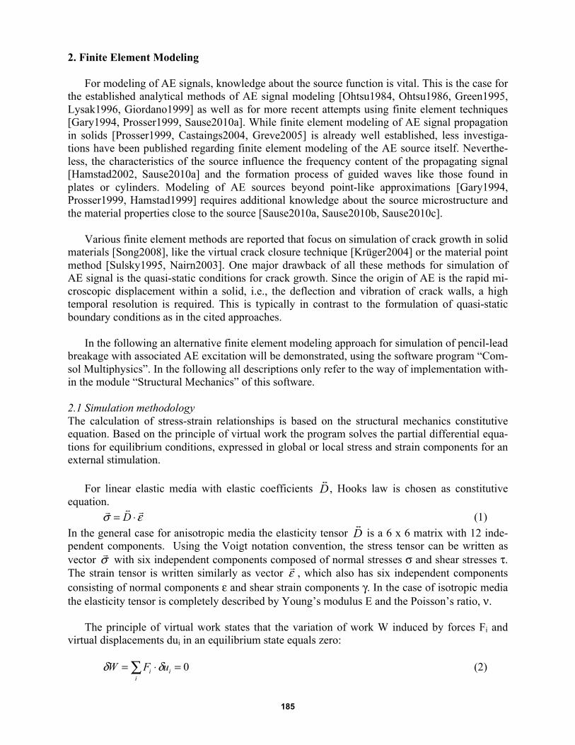
2. Finite Element Modeling For modeling of AE signals, knowledge about the source function is vital. This is the case for the established analytical methods of AE signal modeling [Ohtsu1984, Ohtsu1986, Green1995, Lysak1996, Giordano1999] as well as for more recent attempts using finite element techniques [Gary1994, Prosser1999, Sause2010a]. While finite element modeling of AE signal propagation in solids [Prosser1999, Castaings2004, Greve2005] is already well established, less investiga-tions have been published regarding finite element modeling of the AE source itself. Neverthe-less, the characteristics of the source influence the frequency content of the propagating signal [Hamstad2002, Sause2010a] and the formation process of guided waves like those found in plates or cylinders. Modeling of AE sources beyond point-like approximations [Gary1994, Prosser1999, Hamstad1999] requires additional knowledge about the source microstructure and the material properties close to the source [Sause2010a, Sause2010b, Sause2010c]. Various finite element methods are reported that focus on simulation of crack growth in solid materials [Song2008], like the virtual crack closure technique [Krüger2004] or the material point method [Sulsky1995, Nairn2003]. One major drawback of all these methods for simulation of AE signal is the quasi-static conditions for crack growth. Since the origin of AE is the rapid mi-croscopic displacement within a solid, i.e., the deflection and vibration of crack walls, a high temporal resolution is required. This is typically in contrast to the formulation of quasi-static boundary conditions as in the cited approaches. In the following an alternative finite element modeling approach for simulation of pencil-lead breakage with associated AE excitation will be demonstrated, using the software program “Com-sol Multiphysics”. In the following all descriptions only refer to the way of implementation with-in the module “Structural Mechanics” of this software. 2.1 Simulation methodology The calculation of stress-strain relationships is based on the structural mechanics constitutive equation. Based on the principle of virtual work the program solves the partial differential equa-tions for equilibrium conditions, expressed in global or local stress and strain components for an external stimulation. For linear elastic media with elastic coefficients D

, Hooks law is chosen as constitutive

equation. εσ ⋅= D (1)

In the general case for anisotropic media the elasticity tensor D

is a 6 x 6 matrix with 12 inde-pendent components. Using the Voigt notation convention, the stress tensor can be written as vector σ with six independent components composed of normal stresses σ and shear stresses τ. The strain tensor is written similarly as vector ε , which also has six independent components consisting of normal components ε and shear strain components γ. In the case of isotropic media the elasticity tensor is completely described by Young’s modulus E and the Poisson’s ratio, ν. The principle of virtual work states that the variation of work W induced by forces Fi and virtual displacements dui in an equilibrium state equals zero:

∑ =⋅=i

ii uFW 0δδ (2)

186

Generally, the external applied virtual work equals the internal virtual work and in the case of a deformable body with volume V and surface S, results in a deformation state with new internal stress and strain components.

0=⋅−⋅+⋅ ∫∫∫ dVdVFudSFuV

t

VV

t

SS

t σεδδδ (3)

The external applied forces SF

and VF

act on the surface and volume of the body, respectively. The constraint forces within the material are expressed by consistent internal stress σ and strain ε components, with the superscript t indicating the transposed vectors. To extend the principle of virtual work for dynamic systems, mass accelerations are intro-duced. This yields the formulation of the d’Alembert principle, which states that a state of dyna-mic equilibrium exists if the virtual work for arbitrary virtual displacements vanishes. Taking this into account and introducing the material density r equation (3) becomes:

02

2

=⋅∂∂−⋅−⋅+⋅ ∫∫∫∫ dVutudVdVFudSFu

VV

t

VV

t

SS

t

δρσεδδδ (4)

This defines the basic differential equation solved for every finite element. In order to model structural mechanics problems, a suitable geometry and respective boundary conditions have to be defined. 2.2 Model description The model geometry consists of the tip of a mechanical pencil (i.e., Pentel P205), which is com-posed of a fixed (non-sliding) steel collet and the pencil lead. For all simulations, a 2-dimensional setup with plane-strain conditions was used. As illustrated in Fig. 1, the plastic frame of the mechanical pencil is not modeled, since no mechanical or acoustical contribution is expected from this component. In order to simulate pencil-lead breakage, the mechanical pencil is loaded against a test block in the negative y-direction. All values for the elastic properties used in the simulation are summarized in Table 1. The values for a typical high-strength alloy steel and 7075 aluminum alloy were chosen from the built-in material database of the software Com-sol. Since no entry was found for pencil-lead or a respective graphite modification, a different approach was chosen to select its properties. Literature values for graphite-based materials span a broad range of properties for density, elastic modulus and fracture strength [Sakai1983, Sa-kai1988, Allard1991]. Since the exact composition of the pencil-lead used is subject to assump-tions, the material properties reported in Table 1 were validated by experimental data as de-scribed in section 3. As the pencil lead and test block form different entities, contact modeling was used to trans-fer load and displacement between the tip of the pencil lead to the test block. Since contact mo-deling is restricted to boundary elements, it was necessary to chamfer one of the pencil-lead ed-ges to yield an angled boundary as illustrated in Fig. 1. For all investigations, the length of the chamfer was kept constant at 0.1 mm. The modeling approach to simulate crack growth within the pencil-lead is illustrated in Fig. 2. Initially, the steel collet and pencil lead form a union and are loaded in negative y-direction. At the time of fracture tfrac the internal boundary conditions of the pencil-lead at the tip of the collet are released and contact modeling is enabled. Thus for times t ≥ tfrac both boundaries of the

187

Fig. 1. Illustration of model geometry.

Table 1. Material properties used for simulation.

Property Aluminum Pencil lead Steel Density [Mg/m³] 2.720 1.780 7.850

Elastic modulus [GPa] 71.1 10.5 200.0 Poisson’s ratio 0.33 0.33 0.33

pencil lead are allowed to move independently but do not penetrate each other. The position for separation of the pencil lead was chosen based on static loading of the mechanical pencil. As indicated by the color range of the von-Mises stress in Fig. 2 the maximum stress occurs at the position, were the pencil lead leaves the collet. This is also the typical position, where fracture is introduced experimentally. For this investigation and all following, the size of the mesh elements was chosen to be less than 0.1 mm and was refined at the interacting boundaries for crack initia-tion and contact modeling to go down to 2.5 µm. As temporal resolution 0.01 µs was found to be sufficient, i.e., no change in the calculated solutions was found for a change in resolution down to 0.001 µs. In reality the time for loading of the mechanical pencil is typically a couple of seconds. Computationally it is not feasible to simulate such long loading times with the accuracy in tem-poral resolution of 0.01 µs. Thus, it was investigated, what loading rate is acceptable to reflect quasi-static loading conditions as faced in the experiment. As long as no time-dependent material law is applied, this condition is fulfilled, if the displacement velocity does not exceed the sound velocity of the material. Thus, any external loading of the structure that results in movements sufficiently slower than the transverse sound velocity of the material can be assumed to ensure quasi-static loading conditions. For the current case a good compromise between this require-ment and the computation time was tfrac = 5 µs based on the convergence of the calculated source functions (see section 4).

force direction

chamfer

steel collet

plastic frame

pencil lead

test block

x

y

188

Fig. 2. Definition of boundary conditions and investigation of fracture zone by static loading. It is worth noting that the present approach is sufficient for modeling of pencil-lead break sources, but not necessarily for modeling of crack propagation. The evolution of the latter is se-verely influenced by plastic deformation of the fracture zone due to crack propagation. In order to take into account such changes and the according interaction with the stress field, more com-prehensive approaches for modeling of crack propagation [Sulsky1995, Nairn2003] have to be extended to allow simultaneous simulation of AE. Also, the von-Mises stress values should be used with care, since their absolute value is influenced by the 2-dimensional representation. For a 3-dimensional model a stronger stress concentration at the position between collet and pencil-lead may be expected. 3. Experimental

In order to validate the proposed modeling approach the rupture force for a variety of PLB

configurations were evaluated. As shown at the bottom of Fig. 3, the mechanical pencil was mounted within tensile jaws. The tip of the lead was pressed against a sensitive load cell with 5-N maximum capacity. As defined in Fig. 3, various free lead lengths and contact angles were investigated. In addition, two lead diameters (0.5 mm and 0.3 mm) of hardness 2H were tested. Dimensions of lead diameter, free lead length and contact angle were measured from images like Fig. 3 using a calibrated optical extensometer. Table 2 holds a summary of the chosen parame-ters and the measurement results.

For comparison a respective simulation of the experimental conditions under static loading

conditions was performed. For this purpose the PLB model described in section 2.2 was loaded to the maximum displacement as measured experimentally. As already mentioned in section 2.2, a broad range of properties for graphite modifications is found in literature [Sakai1983, Sa-kai1988, Allard1991]. Since typical values for pencil leads are beyond the scope of literature, a range of elastic properties was evaluated. For this purpose, the elastic modulus was varied be-tween 9.5 GPa and 13.5 GPa in 0.5 GPa steps and density was varied between 1.50 Mg/m³ and 1.80 Mg/m³ in steps of 20 kg/m³. The best agreement between the calculated force at the pencil-lead tip and experimental values was found for E = 10.5 GPa and ρ = 1.78 Mg/m³. For better

test block

force direction

steel colletmaximum stress

von-Mises [MPa]

pencil lead

contact modeling

dynamic boundary conditions

x

y

von-Mises [MPa]

189

comparison, results of experiment and simulation are shown in Fig. 4 as a scatterplot. Within the experimental range of scatter, the simulation results show good agreement.

Fig. 3. Image of measurement setup.

Table 2. Measured rupture forces of PLB for various lead diameters, contact angles and lead lengths. For comparison, results of a static simulation of the chosen configuration are reported.

1 force exceeds limit of load cell

4. Results and Discussion In the following, results of the conducted numerical studies are presented. In Fig. 5 images of the stress distribution around the pencil lead are shown at distinct time steps before and after fracture. For times less than tfrac the stress at the fracture zone increases. For t ≤ tfrac boundary constraints inhibit independent movement of the lower and upper part of the pencil lead. At t > tfrac boundary conditions at the interface are changed to independent movement using contact modeling. The separation (i.e. cracking) of the pencil lead causes initiation of a flexural wave that propagates along the free pencil lead.

free lead length

mechanical pencil

contact angle

load cell

Diameter [mm]

Contact angle [°]

Lead length [mm]

Force (experimental) [N]

Force (simulation) [N]

0.5

23.5 4.0 1.60 ± 0.07 1.61 3.2 2.08 ± 0.14 2.03 2.4 2.34 ± 0.41 2.66

45° 4.0 2.16 ± 0.14 2.31 3.2 3.25 ± 0.68 2.89 2.4 3.97 ± 0.15 3.84

60° 4.0 3.32 ± 0.12 3.39 3.2 4.03 ± 0.50 4.16 2.4 > 5.001 5.14

0.3 45° 4.4 0.47 ± 0.01 0.48 2.2 1.62 ± 0.36 1.25

190

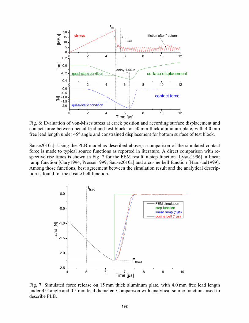
Fig. 4. Comparison of measured rupture forces of PLB configurations and calculated force evaluated at the tip of the pencil lead from the simulation against the angle and free length. Due to inertial forces, the free pencil lead remains in contact with the test block. For a free lead length of 4 mm the flexural wave reaches the tip of the pencil lead within 1.5 µs after frac-ture initiation. At this time the maximum compressive contact force is reached at the tip of the lead. Due to reflection of the flexural wave at the interface between pencil lead and test block, the contact between both is lost. As a consequence, the pencil lead flips away. In Fig. 6, the maximum of the von-Mises stress at the position of the crack within the pencil lead is shown together with the calculated contact force and surface displacement of the test block at the position of the lead tip. Until the time of fracture initiation tfrac the stress at the inter-nal boundary within the pencil lead is increasing linearly, since the pencil is loaded with constant force per time. At t = tfrac boundary conditions are changed and contact modeling is enabled. This causes a sharp drop of the von-Mises stress at this boundary that reaches a steady-state friction stress level after a characteristic time tcrack between 150 ns and 400 ns. This corresponds well to the characteristic times for shear waves propagating across the diameter of the pencil-lead as reported by Scruby et al. [Scruby1978]. The friction stress level originates from the friction con-tact between both boundaries of the pencil lead. As already seen in Fig. 5, a flexural wave propa-gates along the free pencil-lead and reaches the test block delayed by 1.44 µs for 4.0 mm lead length. At this time the maximum surface displacement and the maximum contact force is calcu-lated.

Under quasi-static loading conditions, i.e. a couple of seconds loading time, the initial slope of surface displacement and contact force can be assumed to vanish. This is indicated in Fig. 6 by the dashed horizontal lines. Thus the true source function for a PLB should include a small compressive surface displacement and compressive force at the beginning. It is noted, that source functions for pencil-lead breaks as deduced from experimental signals by deconvolution proce-dures using Green’s theorem yield quite similar signals (see Breckenridge et al. [Brecken-ridge1990]). Also, the signal calculated for the surface displacement is in good agreement to the reports of various other authors [Scruby1978, Breckenridge1990]. The distortion of the contact

23.5

°- 4

.0

23.5

°- 3

.2

23.5

°- 2

.4

45.0

°- 4

.0

45.0

°- 3

.2

45.0

°- 2

.4

60.0

°- 4

.0

60.0

°- 3

.2

60.0

°- 2

.4 --

45.0

°- 4

.4

45.0

°- 2

.2

0.00.51.01.52.02.53.03.54.04.55.05.56.06.5

experimental simulation

rupt

ure

forc

e [N

]

0.5mm lead 0.3mm lead

191

force signal around 7.4 µs is caused by the settings for contact modeling. Depending on the exact parameters chosen within the software, the distortion is emphasized or gets negligible. It is thus considered to be a numerical issue, rather than a physical effect.

Fig. 5. Stress distribution in vicinity of pencil-lead at distinct time steps before and after fracture. Simulation for 4.0 mm free lead length under 45° contact angle. For the purpose of visualization, deformations are exaggerated by a factor of 10. 4.1 Comparison to analytical source functions Most of the time analytical source functions are used to introduce acoustic emission sources for numerical or analytical calculations [Gary1994, Lysak1996, Prosser1999, Hamstad1999,

force direction von-Mises [MPa] von-Mises [MPa]

t = 1.0µs t = tfrac = 5.0µs

von-Mises [MPa] von-Mises [MPa]

t = 5.5µs t = 8.5µs

von-Mises [MPa] von-Mises [MPa]

t = 9.0µs t = 13.0µs

free boundary

flexural wave

pencil lead flips away

stress wave

flexural wave

192

Fig. 6: Evaluation of von-Mises stress at crack position and according surface displacement and contact force between pencil-lead and test block for 50 mm thick aluminum plate, with 4.0 mm free lead length under 45° angle and constrained displacement for bottom surface of test block. Sause2010a]. Using the PLB model as described above, a comparison of the simulated contact force is made to typical source functions as reported in literature. A direct comparison with re-spective rise times is shown in Fig. 7 for the FEM result, a step function [Lysak1996], a linear ramp function [Gary1994, Prosser1999, Sause2010a] and a cosine bell function [Hamstad1999]. Among those functions, best agreement between the simulation result and the analytical descrip-tion is found for the cosine bell function.

Fig. 7: Simulated force release on 15 mm thick aluminum plate, with 4.0 mm free lead length under 45° angle and 0.5 mm lead diameter. Comparison with analytical source functions used to describe PLB.

0 2 4 6 8 10 1205

101520

quasi-static condition

delay 1.44µs

tfrac

contact force

stress

[MP

a]

surface displacement

friction after fracturetcrack

quasi-static condition

0 2 4 6 8 10 12-0.4

-0.2

0.0

0.2 [n

m]

0 2 4 6 8 10 12

-2.0-1.5-1.0-0.50.0

[N]

Time [µs]

4 5 6 7 8 9 10-2.5

-2.0

-1.5

-1.0

-0.5

0.0

Fmax

Load

[N]

Time [µs]

FEM simulation step function linear ramp (1µs) cosine bell (1µs)

tfrac

193

Next, a comparison is shown in Figs. 8-a and -b for the calculated surface displacement sig-nals and surface displacement velocity signals obtained from a 15-mm thick plate at a distance of 40 mm away from the simulated PLB. In both figures the black curve shows the signals obtained using the full PLB model as described above. The same plate geometry was loaded at a point corresponding to the midpoint of the chamfer as seen in Fig. 1. As source functions, the linear ramp function and the cosine bell shape were chosen. In both cases a cosine load function was used to reflect the loading conditions for times t < 6.5 µs (see Fig. 7). In experiments the loading occurs under quasi-static conditions, so this contribution is assumed to be negligible in the final shape of the AE signal. Since only negligible difference is found for the simulated surface dis-placement in Fig. 8-a, the surface displacement velocity was evaluated. Here, minor differences are observed between the PLB model result and the simulations using analytical descriptions. Based on this comparison a slightly better match between 25 µs and 30 µs is found for the de-scription using the cosine bell function. The main difference between the PLB model results and the source model descriptions is attributed to the contribution of friction as seen from Fig. 6.

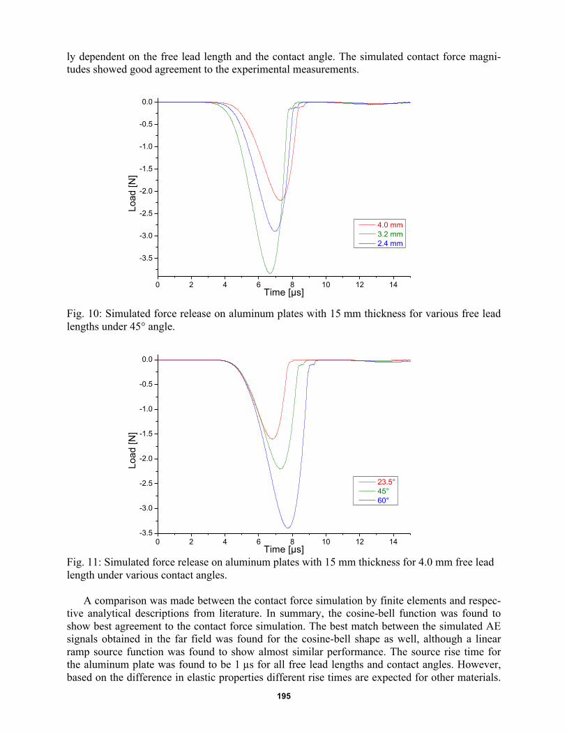
Fig. 8: Comparison of acoustic emission signal from PLB modeling and respective source model descriptions. Surface displacement signal at 40 mm distance from PLB (a) and respective surface displacement velocity (b). 4.2 Variation of test geometry Since PLBs introduce external loads, it is important to consider the boundary conditions for the test block geometry. Since no displacement constraints act on the surface of the test block it gets accelerated through the load introduced by the PLB. This effect is shown in Figs. 9-a and -b, respectively. While the calculated contact force is almost independent of the plate thickness, the situation is different for the calculated surface displacement. Here, mass inertia dominates the simulated surface displacement curves. That is, for larger masses, the surface displacement re-sponse approaches the ideal (constrained) shape as seen from Fig. 6. Thus, for simulations using global coordinate systems, a description of PLBs as load functions is preferred to displacement functions. 4.3 Variation of free lead length As demonstrated experimentally, the variation of free lead length causes different rupture forces. Figure 10 shows the simulated contact forces for the three different lead lengths used experimen-tally. The simulations were for a 15-mm thick plate under 45° contact angle. As already expected from the quasi-static simulations, the maximum load introduced at the contact between pencil-lead tip and test block is dependent on the lead length. Also, the time of maximum load is

0 20 40 60 80 100-600

-500

-400

-300

-200

-100

0

100 PLB model result linear ramp cosine bell

Sur

face

dis

plac

emen

t [nm

]

Time [µs]

(a)

0 20 40 60 80 100-40

-35

-30

-25

-20

-15

-10

-5

0

5

10

15

(b)

Sur

face

dis

plac

emen

t vel

ocity

[mm

/s]

Time [µs]

PLB model result linear ramp cosine bell

194

Fig. 9: Simulated force release on aluminum plates with varying thickness (a) and respective surface displacements (b). All simulations for 4.0 mm free lead length under 45° angle. dependent on the free lead length. This corresponds to the occurrence of the flexural wave as shown in Fig. 6. The arrival time of the wave is obviously linked to the propagation length, which is the length of the pencil lead in this case. The observed difference in arrival times of 0.6 µs for 4.0-mm lead length and 2.4-mm lead length corresponds well to the expected sound velocity for the pencil lead. 4.4 Variation of contact angle Also similar to the experiments, the contact angle between test block and pencil-lead was varied. Figure 11 shows the respective simulations for contact forces under 23.5°, 45.0° and 60.0° con-tact angles. Similar to the variation of free lead length changes in the force magnitudes are ob-served. Also, a shift of the arrival times of maximum contact force is found for the three contact angles. Both observations are attributed to the change in structural loading conditions, i.e., stiff-ness of the mechanical pencil and the pencil lead under vertical loading. It is worth noting that no substantial changes of the contact force shape were found for the variation of free lead length and variation of contact angle. If the obtained curves are normalized and shifted with respect to their maximum, the falling slope understood as source function in Fig. 7 coincides well for all configurations. Thus, the shape of the source function itself is not affect-ed by variation of free lead length or contact angle, but the magnitude of the excited AE signals will directly depend on the magnitude of the contact force. 5. Conclusions The current study contributes to the description of pencil-lead breaks as AE sources. It was demonstrated, that slight differences in the usage of mechanical pencil can introduce large differ-ences in the source magnitude. This was confirmed experimentally by measurement of the rup-ture forces under various contact angles and free lead lengths. A new finite element modeling approach was set up to dynamically change boundary condi-tions that simulate crack propagation within a pencil lead. Within the numerical studies, it was observed how cracking of the lead causes the respective contact forces and surface displacements between pencil-lead tip and test block geometry. It was concluded that a flexural wave propagat-ing along the pencil lead causes a characteristic delay between the time of fracture and the max-imum contact force and surface displacement. The change in delay was found to be systematical-

195

ly dependent on the free lead length and the contact angle. The simulated contact force magni-tudes showed good agreement to the experimental measurements.

Fig. 10: Simulated force release on aluminum plates with 15 mm thickness for various free lead lengths under 45° angle.

Fig. 11: Simulated force release on aluminum plates with 15 mm thickness for 4.0 mm free lead length under various contact angles. A comparison was made between the contact force simulation by finite elements and respec-tive analytical descriptions from literature. In summary, the cosine-bell function was found to show best agreement to the contact force simulation. The best match between the simulated AE signals obtained in the far field was found for the cosine-bell shape as well, although a linear ramp source function was found to show almost similar performance. The source rise time for the aluminum plate was found to be 1 µs for all free lead lengths and contact angles. However, based on the difference in elastic properties different rise times are expected for other materials.

0 2 4 6 8 10 12 14

-3.5

-3.0

-2.5

-2.0

-1.5

-1.0

-0.5

0.0

4.0 mm 3.2 mm 2.4 mm

Load

[N]

Time [µs]

0 2 4 6 8 10 12 14-3.5

-3.0

-2.5

-2.0

-1.5

-1.0

-0.5

0.0

23.5° 45° 60°

Load

[N]

Time [µs]

196

Thus, similar investigations should be conducted to derive rise times for other materials. Ulti-mately, a substitution of the complex source model for pencil-lead breakage by analytical source functions seems appropriate given the computational efficiency and ease of implementation. Acknowledgments I would like to thank Marvin A. Hamstad for the fruitful discussions on simulation of acous-tic emission signals and the recommendations regarding modeling of pencil-lead breakage. References [Allard1991] B. Allard, D. Rouby and G. Fantozzi (1991), Carbon, 29:3, 457-468. [Breckenridge1990] F.R. Breckenridge, T.M. Proctor, N.N. Hsu, S.E. Fick and D.G. Eitzen

(1990), Progress in Acoustic Emission V, eds. K. Yamagushi, H. Taka-hashi, and H. Niitsuma (Eds.), Tokyo, pp. 20-37.

[Castaings2004] M. Castaings, C. Bacon, B. Hosten and M. V. Predoi (2004), J. Acoust. Soc. Am., 115:3, 1125-1133.

[Gary1994] J. Gary and M.A. Hamstad (1994), J. Acoustic Emission, 12:3-4, 157-170. [Green1995] E. R. Green (1995), Composites Engineering, 5, 1453-1469. [Greve2005] D.W. Greve, J.J. Neumann, J.H. Nieuwenhuis, I.J. Oppenheim, N.L. Tyson

(2005), Proc. SPIE, SPIE-5765, pp. 281-292. [Giordano1999] M. Giordano, L. Condelli and L. Nicolais (1999), Comp. Sci. Technol., 59,

1735-1743. [Hamstad1999] M.A. Hamstad, A. O’Gallagher and J. Gary (1999), J. Acoustic Emission,

17:3-4, 97-110. [Hsu1981] N.N. Hsu, F.R. Breckenridge (1981), Mat. Eval., 39, 60-68. [Krüger2004] R. Krüger (2004), Appl. Mech. Rev. 57:2 109-143. [Lysak1996] M. Lysak (1996). Eng. Frac. Mech., 55:3, 443-452. [Nairn2003] J.A. Nairn (2003), Comput. Method. Appl. M., 4, 649-663. [Ohtsu1984] M. Ohtsu and K. Ono (1984), J. Acoustic Emission, 3, 27-40. [Ohtsu1986] M. Ohtsu and K. Ono (1986), J. Acoustic Emission, 5, 124-133. [Prosser1999] W. H. Prosser, M. A. Hamstad, J. Gary and A. O’Gallagher (1999), J.

Nondest. Eval. 18:3, 83-90. [Sakai1983] M. Sakai, K. Urashima and M. Inagaki (1983), J. Am. Ceram. Soc., 66:12,

868-873. [Sakai1988] M. Sakai, J.-I. Yoshimura, Y. Goto and M. Inagaki (1988), J. Am. Ceram.

Soc., 71:8, 609-616. [Sause2010a] M.G.R. Sause and S. Horn (2010), J. Nondest. Eval., 29:2, 123-142. [Sause2010b] M.G.R. Sause and S. Horn (2010), J. Acoustic Emission, 28, 142-154. [Sause2010c] M.G.R. Sause (2010), Identification of failure mechanisms in hybrid mate-

rials utilizing pattern recognition techniques applied to acoustic emission analysis, PhD-thesis, mbv-Verlag, Berlin.

[Scruby1978] C.B. Scruby and H.N.G. Wadley (1978), J. Phys. D. Appl. Phys, 11, 1487-1494.

[Song2008] J.-H. Song, H. Wang and T. Belytschko (2008). Comput. Mech. 42, 239-250.

[Sulsky1995] D. Sulsky, S.-J. Zhou and H. Schreyer (1995), Comput. Phys. Commun. 87, 236-252.