The Pennsylvania State University

The Graduate School

College of Engineering

INVESTIGATION OF NOISE FROM ELECTRIC, LOW-TIP-SPEED

AIRCRAFT PROPELLERS

A Thesis in

Aerospace Engineering

by

Bolor-Erdene Zolbayar

© 2018 Bolor-Erdene Zolbayar

Submitted in Partial Fulfillment

of the Requirements

for the Degree of

Master of Science

August 2018

The thesis of Bolor-Erdene Zolbayar was reviewed and approvedú by the following:

Kenneth S. Brentner

Professor of Aerospace Engineering

Thesis Advisor

Sven Schmitz

Associate Professor of Aerospace Engineering

Jack W. Langelaan

Associate Professor of Aerospace Engineering

Director of Graduate Programs

úSignatures are on file in the Graduate School.

ii

Abstract

This thesis focuses on propeller noise considerations that would be appropriate for a6-9 passenger low-tip-speed, electric propeller-driven aircraft. A baseline aircraft andpropeller are used for reference, but all the propellers evaluated in this work havebeen designed for appropriate tip speeds considered. Electric motors are lighter thanconventional combustion engines. They also can operate at low-tip-speed more e�ectivelythan conventional internal combustion engines. These characteristics allow aircraft tohave multiple low-tip-speed propellers, which can result in a reduction in propeller noise.In this research, the noise of isolated propellers designed for low Mtip=0.3 and 0.4 wasinvestigated and compared with noise of a baseline propeller designed for Mtip=0.7 forthe same thrust and forward aircraft speed.

The design and analysis code CROTOR is used to design all the propellers in thiswork. The lower tip speed reduces the noise considerably, but the individual noise sourcestend to not scale with tip Mach number in the same way. With steady axisymmetricinflow at the level flight condition, the maximum propeller noise is always found in thepropeller plane. To study the relationship between propeller noise and tip speed, isolated3 and 6-bladed propellers are designed for various tip speeds. (Mtip = 0.3, 0.4, 0.5, 0.6,and 0.7). For steady level flight cases, the noise in the propeller plane is found to be thehighest and is found to have a linear relationship with blade tip speed.

Unsteady loading is implemented as an approximation to the loading propellerexperiences when it operates at an angle of attack. The e�ect of unsteady loading isshown to change the directivity of the noise distribution substantially in the plane ofthe propeller and to impact the ultimate noise reduction achievable through tip speedreduction, especially for low-tip-speed designs. In particular, along with the propeller axisof rotation, the noise levels do not change significantly with tip speed, while in the planeof the propeller, the noise reduction with reduced tip Mach number is promising. However,with higher angles of attack, the noise below the propeller increases substantially, and itsdirectivity rotates approximately by the angle of attack –.

Increasing the number of blades can result in significant noise reduction in theplane of rotation (up to 25 dB), but practical limits on the number of blades shouldbe investigated. Distributed electric propulsion system makes it feasible to use several

iii

smaller propellers. So, configurations with 1, 2, 4, and 6-propellers designed in CROTORcode were considered. In the plane of rotation, the noise directivity becomes increasinglycomplex with an increasing number of propellers and the noise directivity can be shapedinto "loud" and "quiet" directions.

These results are aimed to give some direction that could be helpful to design engineersand to demonstrate how current design and analysis tools can be used in a fast andsimple manner to obtain propeller noise predictions.

iv

Contents

List of Figures vii

List of Tables x

List of Symbols xi

Acknowledgments xiv

Chapter 1

Introduction 1

1.1 Motivation . . . . . . . . . . . . . . . . . . . . . . . . . . . . . . . . . . . 11.2 Thesis Objective . . . . . . . . . . . . . . . . . . . . . . . . . . . . . . . . 41.3 Contributions . . . . . . . . . . . . . . . . . . . . . . . . . . . . . . . . . . 5

Chapter 2

Aeroacoustic Theory 6

2.1 Ffowcs Williams and Hawkings Equation (FW-H) . . . . . . . . . . . . . . 72.2 Farassat’s Formulation 1A . . . . . . . . . . . . . . . . . . . . . . . . . . . 82.3 Propeller Noise Sources . . . . . . . . . . . . . . . . . . . . . . . . . . . . 10

2.3.1 Harmonic Noise . . . . . . . . . . . . . . . . . . . . . . . . . . . . . 112.3.2 Broadband Noise . . . . . . . . . . . . . . . . . . . . . . . . . . . . 11

2.4 Summary . . . . . . . . . . . . . . . . . . . . . . . . . . . . . . . . . . . . 12

Chapter 3

Noise Prediction Approach 13

3.1 CROTOR . . . . . . . . . . . . . . . . . . . . . . . . . . . . . . . . . . . . 143.1.1 Blade Element Method and Minimum Induced Loss . . . . . . . . 143.1.2 Blade Loading Calculation . . . . . . . . . . . . . . . . . . . . . . 17

3.2 PSU-WOPWOP . . . . . . . . . . . . . . . . . . . . . . . . . . . . . . . . 193.3 Propeller Design Strategy . . . . . . . . . . . . . . . . . . . . . . . . . . . 20

v

Chapter 4

Results and Discussion 23

4.1 Prediction Set-up . . . . . . . . . . . . . . . . . . . . . . . . . . . . . . . . 234.2 E�ect of Key Parameters on Single Propeller Noise . . . . . . . . . . . . . 26

4.2.1 Significance of Unsteady Loading . . . . . . . . . . . . . . . . . . . 304.2.2 E�ect of Tip Speed . . . . . . . . . . . . . . . . . . . . . . . . . . . 334.2.3 E�ect of Number of Blades . . . . . . . . . . . . . . . . . . . . . . 384.2.4 E�ect of Lift Coe�cient on Noise . . . . . . . . . . . . . . . . . . . 434.2.5 E�ect of Hub Radius on Noise . . . . . . . . . . . . . . . . . . . . 44

4.3 E�ect of Multiple Propellers . . . . . . . . . . . . . . . . . . . . . . . . . . 45

Chapter 5

Concluding Remarks 50

5.1 Conclusions . . . . . . . . . . . . . . . . . . . . . . . . . . . . . . . . . . . 505.2 Recommendations for Future Work . . . . . . . . . . . . . . . . . . . . . . 51

References 53

vi

List of Figures

1.1 Modern and future electric propeller driven aircraft and eVTOL passengerair vehicles . . . . . . . . . . . . . . . . . . . . . . . . . . . . . . . . . . . 2

2.1 Illustration for advanced and retarded time [11,27]. . . . . . . . . . . . . . 10

3.1 Key steps in noise prediction . . . . . . . . . . . . . . . . . . . . . . . . . 143.2 Dividing propeller blade radially into small segments with width of dr and

radius of r [11] . . . . . . . . . . . . . . . . . . . . . . . . . . . . . . . . . 153.3 Airfoil segment at a cross section of propeller blade, showing relationships

between velocity vectors and lift and drag [11] . . . . . . . . . . . . . . . . 153.4 Unsteady loading implementation [16] . . . . . . . . . . . . . . . . . . . . 183.5 Unsteady loading calculation process in noise prediction . . . . . . . . . . 183.6 Propellers at various tip speeds (Mtip=0.3, 0.4 and 0.7) optimally designed

in CRotor . . . . . . . . . . . . . . . . . . . . . . . . . . . . . . . . . . . . 203.7 Configurations with various number of propellers that have same overall

performance . . . . . . . . . . . . . . . . . . . . . . . . . . . . . . . . . . . 213.8 Schematics of the 4, 5 and 6-bladed propellers designed for Mtip = 0.4 . . 22

4.1 Baseline aircraft with its propeller designed in CROTOR. . . . . . . . . . 234.2 Baseline propeller designed in CROTOR. . . . . . . . . . . . . . . . . . . 244.3 Orientation of single propeller . . . . . . . . . . . . . . . . . . . . . . . . . 254.4 Location of observers on X-Z plane . . . . . . . . . . . . . . . . . . . . . . 254.5 Overall sound pressure level (OASPL,dB) polar directivity in the X-Z

plane of a 3-bladed propeller operating at Mtip=0.7 . . . . . . . . . . . . . 264.6 Overall sound pressure level (OASPL, dB) polar directivity in the X-Z

plane of a 3-bladed propeller operating at Mtip=0.7 and acoustic pressuretime history (Pa) plotted at 30 deg increments below the propeller . . . . 27

4.7 Acoustic pressure time history plotted for one revolution for each blade ofthe baseline propeller at elevation angle of 180 deg . . . . . . . . . . . . . 28

4.8 Comparison of steady and unsteady cases by overall sound pressure level(OASPL, dB) on same plot . . . . . . . . . . . . . . . . . . . . . . . . . . 31

vii

4.9 Comparison of steady and unsteady cases by overall sound pressure level(OASPL, dB) polar directivity in the X-Z plane of a 3-bladed propelleroperating at Mtip = 0.7 . . . . . . . . . . . . . . . . . . . . . . . . . . . . 31

4.10 Overall sound pressure level (OASPL, dB) polar directivity in the X-Zplane of a 3-bladed propeller operating at Mtip=0.7 and acoustic pressuretime history (Pa) plotted at 30 deg increments below the propeller . . . . 32

4.11 Comparison of acoustic pressure time history in the direction of polarangle 180 deg between steady and unsteady cases . . . . . . . . . . . . . . 33

4.12 Propellers at various tip speeds (Mtip=0.3, 0.4 and 0.7) optimally designedin CROTOR . . . . . . . . . . . . . . . . . . . . . . . . . . . . . . . . . . 34

4.13 Overall sound pressure level (OASPL, dB) directivity on the X-Z plane forthree tip Mach numbers (0.3, 0.4, 0.7) and two propeller angles of attack(0. and 10 deg). The observer distance is 30 m from the propeller axis. . . 34

4.14 Thickness, loading, and total overall sound pressure level (OASPL, dB)directivity on the X-Z plane for three tip Mach numbers (0.3, 0.4, 0.7)and two propeller angles of attack (0. and 10 deg). The observer distanceis 30 m from the propeller axis. . . . . . . . . . . . . . . . . . . . . . . . . 36

4.15 The noise level at an observer point on the top of propeller (30 m awayfrom propeller hub) in the plane of rotation of 3-bladed and 6-bladedpropellers designed for Mtip = 0.3, 0.4, 0.5, 0.6, and 0.7 . . . . . . . . . . 37

4.16 Schematics of the 4, 5 and 6-bladed propellers designed for Mtip = 0.4 . . 384.17 Comparison of overall sound pressure level (OASPL, dB) directivity in the

X-Z plane for 4, 6, and 8-bladed propellers operating at Mtip = 0.4 andat two di�erent propeller angle of attacks (0 and 10 deg). The observerdistance is 30 m from the propeller axis. . . . . . . . . . . . . . . . . . . . 40

4.18 Acoustic pressure time history of noise components at observer point onthe top of propeller (30 m away from propeller hub) for 4, 6, and 8-bladedpropellers at –=0 and 10deg. . . . . . . . . . . . . . . . . . . . . . . . . . 41

4.19 Acoustic pressure amplitude ratio between single blades and all blades atobserver point on the top of propeller (30 m away from propeller hub) for4, 6, and 8-bladed propellers at – = 0 deg . . . . . . . . . . . . . . . . . . 42

4.20 Overall sound pressure level (OASPL, dB) at observer point on the top ofpropeller (30 m away from propeller hub) for 4, 6, and 8-bladed propellersat – = 0 deg . . . . . . . . . . . . . . . . . . . . . . . . . . . . . . . . . . 43

4.21 Comparison of overall sound pressure level (OASPL, dB) directivity ofnoise components in the X-Z plane for 6-bladed propellers designed for Cl

of 0.5, 0.7, and 0.9 operating at Mtip = 0.4 and at two di�erent propellerangle of attacks (0 and 10 deg). The observer points are 30 m away fromthe propeller hub. . . . . . . . . . . . . . . . . . . . . . . . . . . . . . . . . 44

viii

4.22 Comparison of overall sound pressure level (OASPL, dB) directivity ofthickness, loading, and total noise in the X-Z plane for 6-bladed propellersdesigned for hub radius of 0.05, 0.1, and 0.15 m operating at Mtip =0.4 and at two di�erent propeller angle of attacks (0 and 10 deg). Theobserver points are 30 m away from the propeller hub. . . . . . . . . . . . 45

4.23 Configurations with various number of propellers that have same overallperformance . . . . . . . . . . . . . . . . . . . . . . . . . . . . . . . . . . . 46

4.24 Overall sound pressure level (OASPL, dB) polar directivity plots in theY-Z for 4 di�erent multi-propeller configurations, 0 deg propeller angle ofattack. Note: This is the front view, with the polar angle 0 deg on theport wing of the aircraft, 90 deg above, 180 deg on the starboard wing,and 270 deg below the aircraft. The observer distance is 30 m from thecenterline of the aircraft . . . . . . . . . . . . . . . . . . . . . . . . . . . . 47

4.25 Multi-propeller overall sound pressure level (OASPL, dB) polar directivityin Y-Z plane (front view) for two di�erent propeller angles of attack (0and 10 deg). The observer distance is 30 m from the centerline of theaircraft. . . . . . . . . . . . . . . . . . . . . . . . . . . . . . . . . . . . . . 48

4.26 Multi-propeller overall sound pressure level (OASPL, dB) polar directivityin X-Z plane (side view) for three di�erent propeller angles of attack (0and 10 deg). The observer distance is 30 m from the centerline of theaircraft. . . . . . . . . . . . . . . . . . . . . . . . . . . . . . . . . . . . . . 48

ix

List of Tables

4.1 Input parameters of CROTOR design and analysis code for a baselinepropeller of Tecnam P2012 operating at Mtip=0.7 . . . . . . . . . . . . . . 24

4.2 Input parameters of CROTOR for a propeller operating at Mtip = 0.3 case. 354.3 Input parameters of CROTOR for a propeller operating at Mtip = 0.4 case. 354.4 Input parameters of CROTOR for 4, 6, and 8-bladed propellers operating

at Mtip = 0.4 case. . . . . . . . . . . . . . . . . . . . . . . . . . . . . . . . 394.5 Input parameters of CROTOR for 1-propeller configuration operating at

Mtip=0.4 . . . . . . . . . . . . . . . . . . . . . . . . . . . . . . . . . . . . 494.6 Input parameters of CROTOR for 4-propeller configuration operating at

Mtip=0.4 . . . . . . . . . . . . . . . . . . . . . . . . . . . . . . . . . . . . 494.7 Input parameters of CROTOR for 6-propeller configuration operating at

Mtip=0.4 . . . . . . . . . . . . . . . . . . . . . . . . . . . . . . . . . . . . 49

x

List of Symbols

· Source time

Ab Total blade area

⇤2 Wave operator

c Speed of sound

Cd Coe�cient of drag

Cl Coe�cient of lift

CT Coe�cient of thrust

E Total energy in the spectrum

f = 0 Function that describes source surface

Nb Number of blades

pÕ Acoustic pressure

r Distance between observer and source time

R Propeller blade radius

t/c Thickness to chord ratio

T Propeller thrust

Tij Lighthill stess tensor

U Freestream velocity

Vtip Propeller tip speed

xi

W/A Disk loading

–f Amplification factor

fl Density of medium

dS Element of acoustic data surface

li Local force intensity that acts on the fluid

Pij Compressive stress tensor

pref Reference pressure, 2 ◊ 10≠5Pa

S Spectrum of the normalized pressure fluctuations

t Observer time

ui Component of local fluid velocity

vn Local normal velocity of source surface

x Observer position vector

y Source position vector

Mtip Rotational tip speed Mach number

Abbreviations

UAV Unmanned air vehicle

LEAPtech Leading edge asynchronous propeller technology

BVI Blade-Vortex Interaction

NASA National Aeronautics and Space Administration

DEP Distributed electric propulsion

OASPL Overall sound pressure level

MIL Minimum induced loss

BEM Blade element method

ETHACS Economical thin haul aviation concepts

SPL Sound pressure level

xii

VTOL Vertical take-o� and landing

Subscripts

0 Undisturbed medium

1/3 1/3-octave band

L Loading noise component

n Outward normal vector to the surface

r Radiation direction

ret Retarded time, · = t ≠ r/c

T Thickness noise component

xiii

Acknowledgments

First I would like to thank my adviser, Dr. Kenneth S. Brentner, for helping me everystep of the way and guiding me over the past two years. I also would like to thank mylabmates, Kalki Sharma, Mrunali Botre, Thomas Jaworski, Ajay Singh, and MarianoScaramal for their help and friendship. Lastly, I would like to thank my family for theirlove and support.

This work has been partially supported by the Georgia Institute of Technology aspart of their NASA LEARN project entitled "Economical Thin-Haul Aviation Concepts(ETHACS)" and partially by Penn State. Any opinions expressed within this thesis aresolely those of the authors.

xiv

Dedication

This thesis is dedicated to the memory of my beloved grandmother, Altantsetseg Dambi-inyam.

xv

Chapter 1 |Introduction

1.1 Motivation

Aircraft noise is a key environmental concern in communities and important factor

for health and psychological wellness of flight crew and passengers. Scientists have

determined that stress due to aircraft noise may cause cardiovascular e�ects, sleep

disturbance, conscious and premature awakening, and long-term health problems [1].

Furthermore, aircraft noise may cause negative emotions and cognitive impairment in

children and impact their learning ability [1]. Environmental agencies in Europe suggest

that aircraft noise, a significant part of the environmental noise, is more harmful to

people’s health than passive smoking [2]. Since 1999, the World Health Organization has

recommended aircraft noise in the nighttime should not exceed 45 dB because it increases

the risk of heart attacks, strokes, and dementia [3]. For all these reasons, investigating

the noise from electric, low-tip-speed propellers, has become a subject of intense interest.

In recent years, there has been enormous interest in small electric propeller-driven air-

craft, VTOL (Verical take-o� and landing) passenger vehicles, and small UAVs (Unmanned

air vehicles)/drones. Within a few years, researchers from NASA Langley Research Cen-

ter and Armstrong Flight Research Center plan to fly their DEP (Distributed Electric

Propulsion Driven) X-plane, replacing wings and engines of a Tecnam P2006 with their

improved version of LEAPTech wing technology [4]. The goal of the LEAPTech project

is to help a substantial part of the aircraft industry to make a transition to electrical

1

Figure 1.1. Modern and future electric propeller driven aircraft and eVTOL passenger airvehicles

propulsion within ten years. Furthermore, many potential vehicles have been made or

proposed for the 2-6 passenger vehicle market with a targeted range of less than 200

miles as shown in Fig. 1.1. In 2016, Uber has expressed a strong desire to use small

electric VTOL vehicles as part of their future infrastructure; therefore, creating new

markets [5]. They proposed to launch air taxi networks in Dubai and Dallas as soon as

2020. Furthermore, Uber foresees flight to be a daily part of urban transportation, and

they want to o�er pricing for their electric VTOL aircraft service that is comparable to an

UberX ride. Most large aerospace corporations are investing in the development of small

electric VTOL air vehicles and aircraft to stay competitive in the market; for example,

A3, the Silicon Valley Research and Development outpost of Airbus, has recently tested

its Vahana electric VTOL air vehicle in its first flight [6]. They foresee the future of

transportation as an electric VTOL air vehicle and distributed electric propulsion (DEP)

driven aircraft.

Once these vehicles become a daily part of transportation and a necessity in our lives,

there will be a significant increase in noise emitted to the communities. Thus, low-tip-

speed electric propellers are required, which potentially promise to decrease propeller

noise. Investigating noise from electric, low-tip-speed propellers is an essential task. All

these proposed designs will benefit from significant improvements in battery technology

and electric motor design. Modern electric motors that are expected to have smaller

size and lower weight than conventional combustion engines might allow the vehicles to

2

have multiple low tip-speed propellers. This distributed electric propulsion system can be

used to augment wing lift at low speeds, provide VTOL capability, simplify or eliminate

mechanical controls, and provide low maintenance and redundancy (and hence, safety).

This research work started as an acoustic analysis of Georgia Tech’s project "Eco-

nomical Thin-Haul Aviation Concepts" (ETHACS), which was part of the Leading Edge

Aeronautics Research for NASA (LEARN) program. The goal of the project was to

design 6-9 passenger economically e�cient DEP driven aircraft, which provides low-cost

transportation between small airports [7]. The Tecnam P2012 Traveller aircraft was

chosen as a baseline aircraft for comparison with advanced concepts developed in the

project. The Tecnam P2012 is a twin-engine aircraft with a modern, unswept propeller

design. It carries 6-9 passengers and 1-2 pilots. The aircraft is equipped with 2 Lycoming

TEO-540-C1A engines which each provide 375 hp. The Tecnam P2012 can reach a

maximum cruise speed of 190 kts (100 m/s) and has a maximum takeo� weight of 8000 lb.

One of the most important advantages of using an existing aircraft design as a baseline

aircraft is that data from the baseline aircraft with conventional combustion engines

can be compared to data generated by the exact same model with electric propulsion.

The research focus was based on only the level flight condition with size and operating

condition of the Tecnam P2012 propeller.

Furthermore, a propeller of similar size has been designed with Mtip = 0.7 as a

baseline, and the noise is compared to propellers designed for Mtip = 0.4 and 0.3 values,

for propellers that are expected to be more representative of electric, low tip-speed, low-

noise propellers. To ensure the performance of various tip speed propeller configurations,

the CROTOR code was used to design the propellers used in this work. The design

philosophy used for the comparisons will be explained in more detail in the upcoming

sections. The CROTOR code was also used to provide blade loading for steady and

unsteady loading noise predictions presented in this work.

For conventional aircraft, propellers with thin blades (thickness/chord ratio about

6%) and small camber, the propeller e�ciency only shows a substantial decline for Mtip

> 0.9. However, to keep the noise down to an acceptable level, tip speed must decrease to

have a considerable noise reduction. In fact, the component noise sources do not all vary

3

with Mtip in the same way. Therefore, in this research, the acoustic fields of propellers at

various tip Mach numbers are compared to di�erent configurations that can nominally

perform the same mission, which will be shown in the following chapters.

1.2 Thesis Objective

The focus of this thesis is to investigate noise from low-tip-speed, electric propellers that

can provide guidance to design engineers on how to make low noise electric propellers. To

investigate the propeller noise, the research focuses on the noise distribution of a baseline

single propeller operating with steady inflow at the level flight condition of the baseline

aircraft. To perform that simulation in the noise prediction code PSU-WOPWOP, the

propeller is designed, and its loading and geometry are calculated in CROTOR. Since a

propeller operating with steady inflow is rarely the case in real life, an unsteady loading

calculation methodology is created, and the unsteady loading calculation is performed by

using CROTOR at multiple azimuth (or time) steps. After that, the e�ect of tip speed

is investigated. To do that, low-tip-speed propellers at the same operating condition

are designed in CROTOR and the acoustic results predicted by PSU-WOPWOP are

compared. Then, the e�ect of number of blades, propeller lift coe�cient, and propeller hub

radius are investigated with low-tip-speed designs at the same operating condition. After

all the predictions and analysis, the e�ect of multiple propellers on noise is investigated

because the future eVTOL and DEP aircraft are expected to have multiple propellers.

The following tasks were included in this thesis:

1. Design the baseline propeller of Tecnam P2012 in CROTOR and perform an acoustic

analysis in PSU-WOPWOP.

2. Design low-tip-speed Mtip=0.4 and 0.3 propellers and compare their noise with baseline

propeller noise.

3. Introduce unsteady loading calculation methodology into the acoustic predictions and

compare noise predictions of steady and unsteady inflow cases.

4. Choose important parameters for noise of single single and multiple propellers in

appropriate operating conditions and investigate their significance.

4

5. Design various low-tip-speed single and multiple propeller configurations by changing

the important parameters in appropriate conditions for comparisons and perform an

acoustic analysis on the e�ect of those parameters on the noise.

1.3 Contributions

In general, this research makes three primary contributions based on the tasks above.

1. The change in tip speed due to unsteady inflow was formulated and a quasisteady

approximation that enables the use of CROTOR for unsteady loading computation -

even though it does not compute unsteady loads on its own - was developed. Then, this

unsteady loading was used in PSU-WOPWOP to predict the noise.

2. Low-tip-speed propellers were designed using operating conditions and geometry

representative of the baseline propeller. Noise of various low-tip-speed aircraft propellers

computed with the PSU-WOPWOP noise prediction tool was investigated.

3. The e�ect of critical parameters of propeller noise, including unsteadiness, tip speed,

number of blades per propeller, lift coe�cient, hub radius, and number propellers were

investigated.

5

Chapter 2 |Aeroacoustic Theory

Aeroacoustics is a comparatively new branch of acoustics that studies noise generated

by turbulent fluid motion or aerodynamic forces interacting with surfaces. In short, it

is a study of aerodynamically generated sound. Since the noise is really a propagation

of pressure, it is governed by the conservation laws of fluid mechanics, which includes

conservation of mass, momentum, and energy.

In history, the development of aeroacoustics is driven by research and study of aircraft.

The first theory of aeroacoustics is based on the famous work of Sir James Lighthill and

his "acoustic analogy" in 1952 [8]. The acoustics analogy is directly derived from the

compressible Navier-Stokes equations. Lighthill rearranged the Navier-Stokes momentum

equation into an inhomogeneous wave equation. Although viscous terms are included

in his original analysis, they are usually neglected because they play a negligible role in

noise generation.

In 1969, Ffowcs Williams and Hawkings published "Sound Generation by Turbulence

and Surfaces in Arbitrary Motion," which is an extension of Lighthill’s acoustic analogy

to moving surfaces [9]. The equation they developed is an exact rearrangement of the

continuity and Navier-Stokes equations using generalized functions. They generalized the

"acoustic analogy" and included moving surfaces. With their method, predicting noise

generated by blades of aircraft propellers or helicopter rotors became more feasible.

6

2.1 Ffowcs Williams and Hawkings Equation (FW-H)

The equation of Ffowcs Williams and Hawkings (FW-H) is an exact reformulation of

the Navier-Stokes and continuity equations. Based on their mathematical structure, the

three terms on right side of the Eqn. 2.1, respectively, represent monopole, dipole, and

quadruple terms.

⇤2p

Õ(x, t) = ˆ

ˆt{[fl0Un + fl(un ≠ Un)]”(f)}

≠ ˆ

ˆxi{[Pijnj + flui(un ≠ Un)]”(f)}

+¯2

ˆxiˆxj[TijH(f)]

(2.1)

where x is the observer position and pÕ is the acoustic pressure. The mathematical

notation ⇤2 represents the wave operator and equals to [(1/c

2)( ¯2/ˆt

2)] ≠ O2, where O

2

is the Laplacian, (c - the speed of sound), fl0 represents the density of undisturbed air, n

is a unit normal vector to the surface defined by f = 0. The tensor Pij is the compressive

stress tensor, un and Un represent the component of fluid velocity normal to the surface

and the local normal velocity of the source surface, respectively. The function f implicitly

defines the integration surface; and f has the value.

f < 0 within the surface

f = 0 on the surface

f > 0 outside the surface

(2.2)

Thickness noise and loading noise in Eqn. 2.1 are represented by the monopole and

dipole sources, respectively. The value Dirac delta function, ”(f), is 0 for points not on

the surface. For that reason, thickness and loading noises are restricted to the blade

surfaces. The third component, the quadrupole term, on the other hand, has nonzero

values only outside the surface due to its Heaviside function H(f).

7

H(f) =

Y__]

__[

0 when f<0

1 when f>0(2.3)

Each source term has its physical meaning. The thickness noise due to the monopole

source is generated when blade surface displaces the fluid. The loading noise due to dipole

source is a result of distributed aerodynamic forces on the blade. The quadrupole source

term is responsible for non-linearities due to variation in local sound speed and finite

velocity of fluid near the blade surface. The quadrupole source is the double divergence

of the Lighthill stress tensor, Tij , which is defined as

Tij = fluiuj ≠ Pij ≠ c2(fl ≠ fl0) (2.4)

2.2 Farassat’s Formulation 1A

The advantages of the FW-H equation over CFD methods can be shown using an integral

formulation of the FW-H equation. The importance of the FW-H equation is that it is an

inhomogeneous wave equation for external flow problem embedded in unbounded space;

therefore, the free space Green’s function can be used to find an integral representation

of the solution. Almost all of the rotor noise prediction codes have used integration

formulations developed by Farassat.

In short, Farassat’s Formulation 1A [10] is an integral representation of the solution to

the FW-H equation, (valid for blade surfaces moving at subsonic speeds). The formulation

neglects the quadrupole source term and accounts for the monopole and dipole sources of

the FW-H equation. Elimination of the time derivative of the first integral in Formulation

1 of Farassat speeds up the noise calculation and make it more accurate. Formulation 1A

can be written as

pÕ(x, t) = p

ÕT (x, t) + p

ÕL(x, t) (2.5)

8

where the thickness noise is defined by

4fipÕT (x, t) =

⁄

f=0

Cfl0( .

vn + v .n)

r|1 ≠ Mr|2

D

ret

dS

+⁄

f=0

Cfl0vn(r

.M r + c(Mr ≠ M

2))r2|1 ≠ Mr|3

D

ret

dS

(2.6)

and the loading noise can be written as

4fipÕL(x, t) =1

c

⁄

f=0

C .lr

r|1 ≠ Mr|2

D

ret

dS

+⁄

f=0

5lr ≠ lM

r2|1 ≠ Mr|26

ret

dS

+ 1c

⁄

f=0

Clr(r

.M r + c(Mr ≠ M

2))r2|1 ≠ Mr|3

D

ret

dS

(2.7)

where f = 0 defines the blade surface; the distance between the observer position x and

the source position y is represented by r = |x ≠ y|; vn = v · n is the surface velocity

(f = 0) in the direction normal to itself where n is a unit normal vector to the f = 0

surface; M and Mr represent the Mach number and Mach number component in the

radiation direction of the source surface f=0, respectively; (in the radiation direction

of the surface f = 0); the unit vector pointing to the observer location from the source

location defines the radiation direction. The term lr represents the loading component in

radial direction on surface. While the terms with r≠2 factor are defined as the near-field

terms, the terms with r≠1 factor are defined as the far-field terms because the far-field

terms have a much larger strength than the near-field terms when r is significantly high.

The Doppler amplification factor is represented by 1/(|1 ≠ Mr|).

In Eqns. 2.5, 2.6 and 2.7, the sound at an observer point x and time t is calculated

by integrating over a range of source positions y and time · . The "ret" subscript in

Eqns. 2.6 and 2.7 indicates that the integrands in these equations are evaluated at the

retarded time. This integral formulation is known as a retarded time formulation and

the relationship between the source time, · , and the observer time, t, can be considered

from two viewpoints.

For the first viewpoint (advanced time approach), if the time when the source emits

9

Source Location

Observer Locationr

(x,t)

(y, )

Sonic velocity = c

ω

Figure 2.1. Illustration for advanced and retarded time [11,27].

the sound wave is (·) [18]. Then, by simple calculation, the time when the sound wave

approaches to the observer will be

t = · + r

c(2.8)

where r = |x ≠ y|.

For the second viewpoint (retarded time approach), if the time when sound wave

approaches to the observer be (t) [18]. Then, by simple calculation, the time when the

source emitted the sound wave will be

· = t ≠ r

c(2.9)

The relationship between the source time and observer time is critical in understanding

the sound generation process central to Farassat’s formulation 1A.

2.3 Propeller Noise Sources

There are two types of propeller noise: 1) harmonic noise generated by the propeller,

which repeats at each revolution, and 2) broadband noise, which is caused by unsteady

loading fluctuations due to turbulence ingestion or turbulence in the propeller blade’s

boundary layer.

10

2.3.1 Harmonic Noise

Harmonic noise can be further subdivided into steady and unsteady components, where

steady noise is related to the steady loading on blades (steady in the blade reference

frame) and thickness noise; whereas the unsteady harmonic noise is a result of unsteady

loading on blades and unsteady blade motion (for thickness noise). The primary source

of harmonic noise is directly dependent on operating condition of a propeller and its

rotational speed. Steady loading on the blade surface occurs when the propeller is

operating in a completely clean and axisymmetric steady inflow. The force components of

steady (constant) lift and drag of the blade in the direction of an observer point change

as the propeller rotates, resulting in an unsteady pressure fluctuation that is felt at the

observer location. However, in the real world, most propellers operate in a non-uniform

inflow due to angle of attack of the propeller, some other inflow distortion, or under the

influence of various unsteady aerodynamics mechanisms - all of which lead to increased

noise beyond the "steady" harmonic noise. In this work, a simple quasisteady model of

the unsteady loading for a propeller operating at an angle of attack is used as a surrogate

of more general unsteady loading.

2.3.2 Broadband Noise

Broadband noise is caused by the interaction between a blade and turbulent flow. In other

words, the randomly fluctuating force on the propeller due to turbulent flow generates the

noise. Propeller broadband noise may be comparatively smaller than the harmonic noise,

but it is more di�cult to predict by first principles, and empirical methods are not as

reliable outside of their normal area of application. For these reasons, the broadband noise

is ignored in this thesis, but it could be quite important for small UAV propellers and

low-tip-speed propellers. Nevertheless, if the unsteady loading is found to be significant,

broadband noise is a form of unsteady loading; therefore, the unsteady loading noise

results given here may give some insight into the importance of broadband noise in the

cases considered.

11

2.4 Summary

A brief history and background of aeroacoustics was presented. Then, the equation

of Ffowcs Williams and Hawkings was explained. It is an exact reformulation of the

Navier-Stokes and continuity equations into an inhomogeneous wave equation. With

Ffowcs Williams and Hawkings equation, predicting noise generated by propeller or rotor

blades became more practical. After that, Farassat’s Formulation 1A was explained. It

is an integral representation of the FW-H equation. Most of the rotor noise prediction

codes uses the integration formulation developed by Farassat. Finally, two main propeller

noise sources are explained: harmonic and broadband noise. This thesis focuses on

harmonic noise which consists of loading and thickness noise. This theoretical background

information will be helpful to understand the noise prediction results.

12

Chapter 3 |Noise Prediction Approach

In this section, the noise prediction process will be described, with some of the unique

details given more attention. The PSU-WOPWOP acoustics prediction tool [17–19] uses

the Ffowcs Williams-Hawkings (FW-H) equation [9] and applies Farassat’s Formulation

1A [10] for integration to predict acoustic pressure. A chordwise compact approximation

[17–19] (an option in PSU-WOPWOP) is used in this thesis’ noise prediction process.

This approximation enables the direct use of propeller blade section loading from other

analysis tools to be used for the loading noise prediction. The full surface geometry of

the propeller is used for the thickness noise predictions. To prepare the input data for

PSU-WOPWOP, the blade surface geometry of propeller is generated using four airfoil

sections of the baseline propeller blade and its blade loading is calculated in the design

and analysis tool CROTOR [12]. The CROTOR code takes an input of number of blades,

blade radius, hub radius, hub wake displacement body radius, airspeed, thrust, rotational

speed, and blade lift coe�cient of the propeller. To prepare the output data of CROTOR

in a format of PSU-WOPWOP input, Thomas Jaworski and Ryan Mcconnell wrote an

interface code. The interface code is also used for unsteady loading calculation. The

interface code uses the CROTOR to generate approximate quasi-steady loading for the

propeller. The code divides the propeller disk into 30 equally spaced azimuth stations

and calculates a tip speed at each station considering the unsteady inflow with an angle of

attack of –. Then, the CROTOR is run at each station to calculate the blade loading at

each location. At last, the output data of the interface code is input into PSU-WOPWOP,

13

which outputs acoustic pressure time history and OASPL at observer points. The overall

key steps for the noise prediction in summed up in Fig. 3.1

Figure 3.1. Key steps in noise prediction

In the following sections, the noise prediction approach and its tools are explained in

detail.

3.1 CROTOR

CROTOR is a code that designs and analyzes ducted and free-tip propellers [12]. The

CROTOR uses minimum induced loss (MIL) and blade element method (BEM) and

generates a propeller design within a short time. The concepts of blade element method

and the minimum induced loss are explained briefly in the following sections.

3.1.1 Blade Element Method and Minimum Induced Loss

The fundamentals of the blade element method is explained in this section. In the process

of BEM, the propeller blade is divided into equally spaced small segments along its span

14

in which each segment will have a geometric shape as a function of airfoil, radius, chord,

and blade angle as shown in Fig. 3.2. Then, aerodynamic forces on each of these small

segments are determined. After that, the forces and moments created by the entire

propeller are found by integrating the aerodynamic forces on each small segment along

the entire propeller blade over one rotor revolution.

Figure 3.2. Dividing propeller blade radially into small segments with width of dr and radius ofr [11]

An airfoil segment at a cross section of propeller blade is shown in Fig. 3.3 where VŒ

is the inflow velocity and �r is rotational speed. The segment lift and drag are dL and

dD, respectively. The geometric blade angle is —, and airfoil angle of attack is –.

Figure 3.3. Airfoil segment at a cross section of propeller blade, showing relationships betweenvelocity vectors and lift and drag [11]

V =Ò

V 2a + V

2t =

ÒV 2

Œ + (�r)2 (3.1)

15

With rotational speed and inflow velocity, the total velocity can be found by Eqn. 3.1.

After that, the angle of attack at each section is calculated using the blade angle and

relative wind angle at section as shown in Eqn. 3.2.

„ = arctan(Va

Vt) = arctan(VŒ

�r)

– = — ≠ „

(3.2)

Then, lift and drag at each segment are calculated based on total velocity. With that

information, by simple 2D airfoil analysis, the relationship between lift, drag, and moment

coe�cients can be found. In the next step, local thrust and torque can be represented by

relative wind angle and local lift and drag coe�cients.

dL = 12ClflV

2cdr

dD = 12CdflV

2cdr

dT = dL cos(„) ≠ dD sin(„) = 12flV

2c(Cl cos(„) ≠ Cd sin(„))dr

dQ = (dL sin(„) + dD cos(„))r = 12flV

2c(Cl sin(„) + Cd cos(„))dr

T = B

ÿdT

Q = B

ÿdQ

(3.3)

At the end, total thrust and torque can be found by integrating local thrust torque over

the small sections divided along the blade span as shown in Eqn. 3.3 [11].

Applying the minimum induced loss method for BEM enables to take into account

the finite span e�ect on circulation distribution and viscous drag in performance analysis

[13–15]. BEM is a very simple method because it does not consider that the circulation is

zero at the blade tip and the blade sections a�ect each other. For that reason, CROTOR

uses the minimum induced loss method in BEM in an iterative way. This method of

CROTOR is known as an excellent method of analyzing rotor performance in a quick

and accurate way. For minimum induced loss condition, propeller blade of minimum

induced loss can be seen as a rotating version of minimum induced wing (elliptically

loaded) [13–15]. In that condition, the blade has constant lift to drag ratio radially.

16

Therefore, finding distribution of circulation requires overall lift coe�cient, which is

asked in the input of CROTOR propeller blade design selection. During the design

iteration, CROTOR finds the distribution circulation that agrees with the given overall

lift coe�cient. The MIL of CROTOR is an iterative numerical method, which requires a

valid starting condition for convergence. For blade section analysis, chord, twist angle,

lift and drag coe�cients, airspeed, and rotational speed at each blade section have to be

known.

3.1.2 Blade Loading Calculation

To make an acoustic prediction, the PSU-WOPWOP [17–19] code requires an input of

geometry, loading, and operating condition of propeller blades. The computation of

propeller blade loading was performed with the CROTOR propeller design tool [12]. In

fact, the blades were first designed with CROTOR - to ensure they were reasonable blade

designs for the operating condition - and then the spanwise loading was dimensionalized

and converted into a format required by PSU-WOPWOP. The CROTOR extensions

to XROTOR provide a blade lofting capability that was used to generate the propeller

blade surface geometry needed by PSU-WOPWOP for thickness noise prediction. For

the unsteady loading calculations (propeller at angle of attack or yaw angle), CROTOR

was also used in a simple manner to produce approximate quasi-steady loading for the

propeller. In a steady case, the propeller tip speed around the azimuth is constant.

When introducing an angle of attack, the tip speed varies around the azimuth, as

described by

Vtip = �R + VF sin – sin  (3.4)

where R is propeller radius, � is angular velocity, VF is forward speed, – is propeller

angle of attack, and  is azimuth angle. To model an unsteady flow, the propeller is

analyzed at some fixed number of equally spaced azimuth stations. Each azimuth station

is prescribed a tip speed calculated using Eqn. 3.4 and then CROTOR is run with the

di�erent tip speeds. CROTOR calculates chord length, section Cl and Cd, and twist,

at each spanwise station along the blade (30 span stations used in this paper), which

17

Figure 3.4. Unsteady loading implementation [16]

are used to calculate section lift and drag forces. Next the section lift and drag forces

are used to calculate in-plane and out-of-plane loading forces at each spanwise position

and these loading forces are used in PSU-WOPWOP as periodic loading to predict the

loading noise of the propeller operating at relatively small angles of attack (or yaw). The

unsteady loading calculation process is described in Fig. 3.5

Figure 3.5. Unsteady loading calculation process in noise prediction

18

3.2 PSU-WOPWOP

The PSU-WOPWOP program [17–19] is a robust aeroacoustic prediction tool. The

PSU-WOPWOP program, which is a numerical implementation of Farassat’s Formulation

1A [10] of the Ffowcs Williams-Hawkings equation [9], is used for the prediction of the

harmonic noise generated by the propeller. Formulation 1A, as implemented in PSU-

WOPWOP, is valid in the acoustic near and far fields for arbitrary geometry and subsonic

source motion (the FW-H quadrupole source has been neglected) for stationary and

moving observers. A chordwise compact approximation (an option in PSU-WOPWOP)

has been used in this work, which assumes the propeller is acoustically compact in the

thickness and chordwise directions, but not in the spanwise direction. This approximation

is typically very accurate and enables the direct use of propeller blade section loading

from other analysis tools to be used for the loading noise prediction. For thickness noise

predictions, the full surface geometry of propeller blades is used.

Users input aeromechanical data of aircraft or any other simulated object into PSU-

WOPWOP and it calculates the noise at specified observer locations. Basically, there are

three main steps required to make predictions in PSU-WOPWOP. First, PSU-WOPWOP

requires a geometry data, which has physical location time history of each node for the

noise source. Second, it requires loading data, which has a time history of the load applied

to each node by the fluid. Third, it must have a flight condition setup, orientation, and

movement of the helicopter rotor or aircraft propeller.

The core of the PSU-WOPWOP code is an object called a "patch" that stores loading

and surface geometry for a single surface. A collection of patches together describe

the acoustic integration surface for the problem. Observer points are responsible for

post-processing and storing the acoustic pressure time histories calculated by the patches.

The observer locations can be represented in many ways ranging from a single stationary

point to a plane and spherical surface surrounding the aircraft or helicopter. In this

research, observer points along an arc of spherical surface are mostly used (observer

points on a circle).

Once the contributions from all patches are summed up for a specific observer point,

19

and the integration is done, post-processing is accomplished. It can be as simple as writing

an acoustic pressure time history or as complex as applying Fast Fourier Transform (FFT)

and calculating the Overall Sound Pressure Level (OASPL). In this research, OASPL

and acoustic pressure time history are mostly used for acoustic analysis.

3.3 Propeller Design Strategy

The Tecnam P2012 Traveller aircraft was used as the inspiration for the baseline propeller

in this study. The P2012 aircraft has two 3-bladed propellers, each with a radius of

approximately 1.05m. For this study, one of the key features is to consider propellers

with di�erent tip Mach numbers, ranging from Mtip = 0.3 to 0.7.

Figure 3.6. Propellers at various tip speeds (Mtip=0.3, 0.4 and 0.7) optimally designed inCRotor

To investigate the e�ect of the tip speed, comparisons between single propellers

designed to operate at Mtip = 0.3, 0.4, and 0.7 are made because one propeller normally

would not be expected to operate e�ciently, even with variable pitch, over such a wide

range of tip speeds. The most important requirement to have reasonable comparison in

acoustic results for all these designs will be that the forward speed, radius, and thrust

are held constant at 51.44 m/s, 1.05 m, and 2800 N, respectively. So, the solidity (chord

distribution and number of blades) and twist distribution vary in these designs to meet

the performance requirements. The propellers designed in CROTOR are shown in Fig.

3.6.

Another key feature of aircraft noise can be the number of propellers. For that reason,

this research will consider the noise from di�erent numbers of propellers ranging from a

single propeller to six propellers (in each configuration the propellers are colinear in a line

20

parallel with the wing). The di�erent configurations with various number of propellers

are shown in Fig. 3.7.

Figure 3.7. Configurations with various number of propellers that have same overall performance

The design philosophy of all these di�erent comparisons is that the noise of di�erent

configurations needs to be compared in a manner that does not change the performance

in an adverse way or is an "unfair" comparison. To address these issues the ability of

CROTOR to design appropriate propellers for the various operating conditions has been

used. All the comparisons in this research will consider a single flight speed of 51.44 m/s

(100 kts). The total thrust and total swept area (for all propellers) are held constant at

5600 N and 6.92 m2, respectively, to have the same performance for each configuration.

As the propeller tip speed is varied, the propeller is redesigned to ensure it is able to

provide nominally the same thrust (5600N total thrust) at the new tip speed. This

typically will involve changing the solidity (blade chord distribution, number of blades,

or both) and potentially the twist distribution.

If the number of propellers on the aircraft is changed, then the total thrust and

total swept area (sum of all the propellers in each case) are held fixed. As the number

of propellers changes, this also implies that the radius of the propellers change, so an

additional constraint is imposed that the tip Mach number is held fixed as well, which

21

means the rotation speed is not the same for propellers of di�erent radii (i.e., when a

di�erent number of propellers are used on the aircraft). These choices ensure that the

forward speed and total thrust of all propellers are fixed for all cases; Mtip changes only

when desired; and the radius of the propellers vary when the number of propellers used

on the aircraft vary. One other point of notation: While it is standard to refer to the

propeller tip Mach number as the velocity of the tip divided by the local speed of sound,

here the notation is that the rotational velocity divided by the undisturbed medium

speed of sound is referred to as Mtip.

Finally, another important feature of aircraft propellers (number of blades per pro-

peller) in noise is analyzed. In this study, propellers with 4, 6, and 8 blades designed

for Mtip=0.4 are compared. To have a reasonable comparison, thrust, swept area, and

forward speed are held constant. As shown in Fig. 3.8, the blade chord is decreased as

the number of blade is increased.

Figure 3.8. Schematics of the 4, 5 and 6-bladed propellers designed for Mtip = 0.4

22

Chapter 4 |Results and Discussion

4.1 Prediction Set-up

The baseline aircraft for this research is an Italian Tecnam P2012 aircraft. It carries

6-9 passengers and 1-2 pilots. It is a modern twin propeller aircraft equipped with 2

Lycoming TEO-540-C1A engines that provide 750 hp in total. The Tecnam P2012 can

reach maximum cruise speed of 190kts (100 m/s) and has a maximum takeo� weight of

8000 lb.

Figure 4.1. Baseline aircraft with its propeller designed in CROTOR.

23

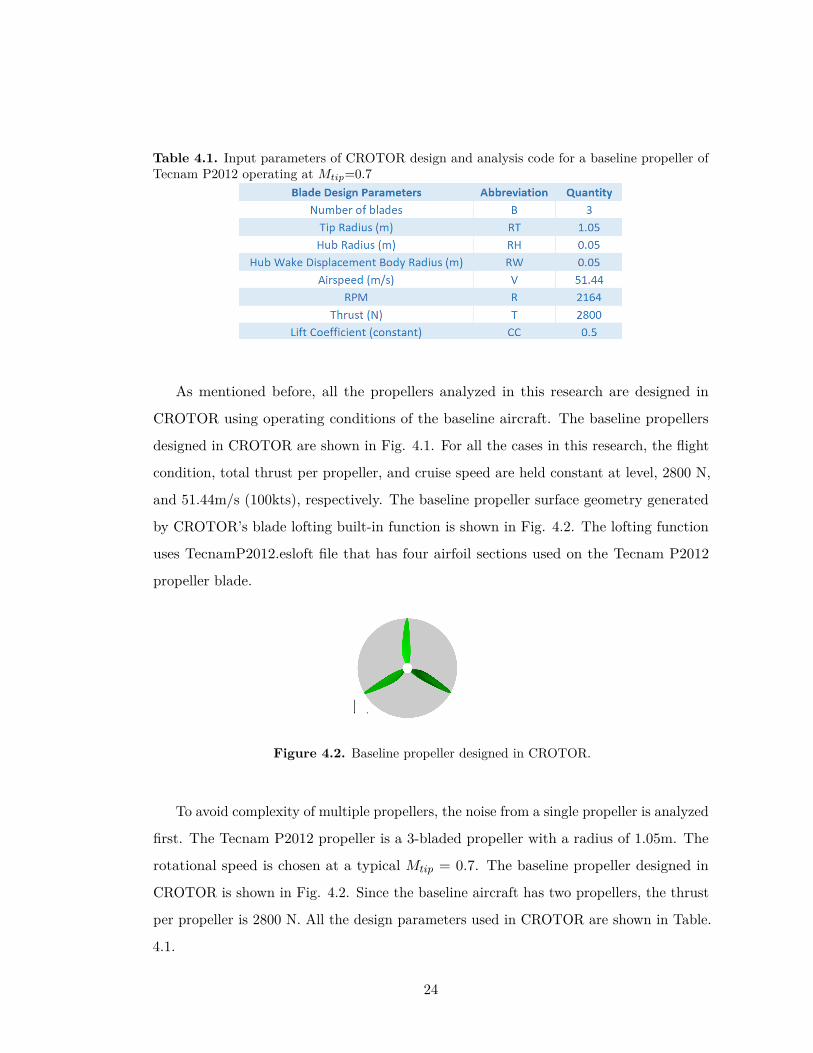
Table 4.1. Input parameters of CROTOR design and analysis code for a baseline propeller ofTecnam P2012 operating at Mtip=0.7

As mentioned before, all the propellers analyzed in this research are designed in

CROTOR using operating conditions of the baseline aircraft. The baseline propellers

designed in CROTOR are shown in Fig. 4.1. For all the cases in this research, the flight

condition, total thrust per propeller, and cruise speed are held constant at level, 2800 N,

and 51.44m/s (100kts), respectively. The baseline propeller surface geometry generated

by CROTOR’s blade lofting built-in function is shown in Fig. 4.2. The lofting function

uses TecnamP2012.esloft file that has four airfoil sections used on the Tecnam P2012

propeller blade.

Figure 4.2. Baseline propeller designed in CROTOR.

To avoid complexity of multiple propellers, the noise from a single propeller is analyzed

first. The Tecnam P2012 propeller is a 3-bladed propeller with a radius of 1.05m. The

rotational speed is chosen at a typical Mtip = 0.7. The baseline propeller designed in

CROTOR is shown in Fig. 4.2. Since the baseline aircraft has two propellers, the thrust

per propeller is 2800 N. All the design parameters used in CROTOR are shown in Table.

4.1.

24

Figure 4.3. Orientation of single propeller

Orientation of the single propeller flying in the -X direction is shown in the Fig. 4.3

where the axis of rotation of the propeller is along the X axis. All the results will be

explained using this orientation in the following sections. The Y-Z plane represents the

plane of rotation of the propeller, and the X-Z plane contains the axis of rotation of

the propeller. In most results, the overall sound pressure level (OASPL) directivity is

presented as a polar plot in the X-Z and Y-Z planes.

Figure 4.4. Location of observers on X-Z plane

To predict the noise in the X-Z plane, 181 observer points are placed on the circle

25

with a 30 m radius centered at the propeller hub, as shown in Fig. 4.4. The propeller is

flying in the -X direction. Each observer on the circle is separated by 2 degrees. This

circular setup is also used to analyze noise distribution in the Y-Z plane. The importance

of this circular setup is that changes in noise due to distance will not a�ect the prediction

because each observer point is 30 m away from the propeller hub. Both the OASPL and

acoustic pressure time history can be studied at the observer locations on the circle in

the X-Z plane.

4.2 E�ect of Key Parameters on Single Propeller Noise

In this section, the impact of changing key parameters of a single propeller on the noise

is investigated. The overall sound pressure level (OASPL) distribution for the baseline,

3-bladed propeller operating with Mtip = 0.7 in axisymmetric 100 kt flight is shown as a

polar plot in the X-Z plane in Fig. 4.5.

Figure 4.5. Overall sound pressure level (OASPL,dB) polar directivity in the X-Z plane of a3-bladed propeller operating at Mtip=0.7

The OASPL levels for the thickness, loading, and total components are plotted as

a function of observer angle in red, blue, and black colors, respectively. Observers are

positioned 30 m from the center of the propeller hub as mentioned in the description

26

of Fig. 4.4. In Fig. 4.5, the polar angle is 0 deg downstream of the propeller and 180

deg upstream, while 90 deg and 270 deg are in the propeller plane. The maximum

OASPL level is found to be approximately 97 dB in the direction of 75 deg and 285 deg,

respectively. In Fig. 4.5, the loading noise is found to be a dominant contributor to

the total OASPL. However, at polar angles around 120 deg and 240 deg, the thickness

noise contributes more than the loading to the total OASPL. The noise in the direction

of 0 deg and 180 deg (on the propeller axis directly downstream and upstream of the

propeller, respectively) is found to be the lowest because this is a steady flight condition

and the propeller inflow and loading are perfectly axisymmetric with respect to the axis

of rotation. This behavior will be compared to the case of unsteady loading, where the

loading is not axisymmetric, in the next section.

Figure 4.6. Overall sound pressure level (OASPL, dB) polar directivity in the X-Z plane of a3-bladed propeller operating at Mtip=0.7 and acoustic pressure time history (Pa) plotted at 30deg increments below the propeller

To investigate the noise more thoroughly, the acoustic pressure time history is shown

27

in Fig. 4.6. The acoustic pressure time histories are shown at elevation angles 30 degrees

apart on the bottom half of the X-Z plane in the figure. One propeller rotation period

is shown in the figure, which is why three blade pulses (for a 3-bladed propeller) are

seen. The acoustic pressure amplitudes are found to be negligible on the propeller axis

(0 deg and 180 deg). As the elevation angle increases from the axis of rotation (180

deg) to the plane of rotation of the propeller (270 deg), the acoustic pressure amplitude

keeps increasing. In fact, acoustic pressure amplitude is largest in the direction of 270

deg. That is not a desirable characteristic because the highest noise is being produced

right below the aircraft, which could a�ect the community the most during flyover. The

acoustic pressure amplitude along the propeller axis (0 deg and 180 deg) is negligible

even though the noise from individual blades is not zero. The reason why noise is so low

on the propeller axis when it is operating in steady inflow can be explained in Fig. 4.7.

Figure 4.7. Acoustic pressure time history plotted for one revolution for each blade of thebaseline propeller at elevation angle of 180 deg

As shown in Fig. 4.7, the acoustic pressure signals from all 3 blades are completely

28

identical because the inflow is steady and axisymmetric. The signal from each blade is

separated by a phase angle of 120 degrees from the other blades. Upon closer examination,

the total acoustic pressure amplitude on the propeller axis actually has three small peaks.

Because the signal from each blade looks similar to sine wave, a simple math expression

(see Eqn. 4.1) can help to explain why the total acoustic pressure signal becomes negligible.

f = sin(x) + sin(x + 120o) + sin(x + 240o)

= sin(x) + sin(60o ≠ x) ≠ sin(60o + x)

= sin(x) + 2 sin (60o ≠ x) ≠ (60o + x)2 cos (60o ≠ x) + (60o + x)

2= sin(x) + 2 sin(≠x) cos(60o)

= sin(x) ≠ sin(x) = 0

(4.1)

In Eqn. 4.1, the sum of the three sine waves is identically zero. This is approximately

the same as the sum of the noise from the three propeller blades. Now, let’s consider this

in a general case with an n-bladed propeller below;

if n = 2k + 1 and a = 360o

n :

f = sin(0) + sin(a) + sin(2a) + ... + sin((n ≠ 1)a)

= sin(a) + sin(2a) + sin(3a) + ... + sin(2ka)

= (sin(a) + sin(2ka)) + (sin(2a) + sin((2k ≠ 1)a)) + ... + (sin(k) + sin(k + 1))

= 2 sin((2k + 1)a2 ) cos((2k ≠ 1)a

2 ) + .. + 2 sin((2k + 1)a2 ) cos(a

2))

= 2 sin((2k + 1)a2 )[cos((2k ≠ 1)a

2 ) + cos((2k ≠ 3)a2 ) + ... + cos(a

2)]

sin((2k + 1)a2 ) = sin(na

2 ) = sin(360o

2 ) = 0

(4.2)

The same proof can be done for the case when n = 2k and it is clear that the noise from

an n-bladed propeller will be negligible along the propeller axis in axisymmetric flow.

In the remainder of the research, the e�ect of unsteady loading, tip Mach number,

number of blades, number of propellers, blade lift coe�cient and propeller’s hub radius

29

will be examined to determine the impact on the noise.

4.2.1 Significance of Unsteady Loading

The primary source of the harmonic noise of the propeller is dependent upon its tip

speed and operating condition. When a propeller operates entirely in steady, clean inflow

aligned with the propeller axis, the propeller blade loading is steady (time independent)

in the blade frame of reference. However, this is rarely the case in typical operation

where the propeller inflow is not completely axisymmetric. In unsteady conditions, the

propeller operates with time-varying inflow; therefore, the angle of attack and velocity

vary both in time and along the span. Such unsteady loading can result in a significant

increase in the noise generated because additional source terms appear in the governing

equations (e.g., the FW-H equation). For example, Gri�th and Revell [20] found that

noise predictions for a low-noise, low-tip-speed propeller were strongly dependent upon

a complete accounting for unsteady loading. The noise was significantly more accurate

when all the sources of unsteady loading were included in the noise predictions. The

unsteady loading calculation is explained in [20].

In this work, when introducing an angle of attack, the tip speed varies around the

azimuth angle of the propeller disk. To model an unsteady flow, the propeller was

analyzed at 30 equally spaced azimuth stations. Each azimuth station  is prescribed a

tip speed calculated using �R+VF sin – sin Â. Then CROTOR is run 30 times with the

di�erent tip speeds at each azimuth station. These loading calculations are input into

PSU-WOPWOP and the OASPL distribution as polar plots in X-Z plane of steady and

unsteady cases are compared in Fig. 4.8. The e�ect of unsteady inflow is represented for

10 deg of angle of attack.

In Fig. 4.8, on the top part of the propeller, the noise in the steady case is substantially

larger than that in the unsteady case. However, the noise is increased significantly - as

much as 6 dB - on the bottom half of the propeller in the unsteady case. The reason that

the noise on the bottom side of the propeller is much larger than that on the top side

of the propeller is that as the propeller rotates downward, the maximum velocity of the

tip is higher due to the angle of attack (�R+VF sin – - at  = 270 deg) than when the

30

Figure 4.8. Comparison of steady and unsteady cases by overall sound pressure level (OASPL,dB) on same plot

blade moves upward, where the angle of attack reduces the velocity (�R-VF sin – - at Â

= 270 deg). This change in velocity as the propeller travels downward or upward results

in a change in Doppler amplification that results in the significant noise di�erence above

and below the propeller. Moreover, it is clear that understanding the e�ect of unsteady

loading more in depth is crucial because it could dramatically increase the noise level

in communities below the flight path. To analyze more in depth, thickness and loading

noise components are plotted with their total in Fig. 4.9.

Figure 4.9. Comparison of steady and unsteady cases by overall sound pressure level (OASPL,dB) polar directivity in the X-Z plane of a 3-bladed propeller operating at Mtip = 0.7

31

As expected, the change in unsteady loading is responsible for the change in total

OASPL. On the other hand, no significant change in thickness noise is observed because

thickness noise is not a function of blade loading. In fact, there is a small shift in the

thickness noise directivity due to the –=10 deg rotation of the propeller. To take a closer

look at the contribution of the unsteady loading, analysis of acoustic pressure time history

is necessary.

Figure 4.10. Overall sound pressure level (OASPL, dB) polar directivity in the X-Z plane of a3-bladed propeller operating at Mtip=0.7 and acoustic pressure time history (Pa) plotted at 30deg increments below the propeller

The acoustic pressure time history has been plotted for the unsteady case at observer

positions below the rotor in Fig. 4.10. Similar to Fig. 4.6, all the acoustic pressure time

history plots have 3 peaks. Also, the acoustic pressure amplitudes are smallest along the

propeller axis. Their magnitudes get larger as they get closer to the propeller’s plane

of rotation. The fact that the pressure amplitudes in the range between 180 and 270

degrees are larger than those in the range between 270 and 360 degrees matches with the

32

OASPL distribution. The reason is that the bottom side with higher noise is tilted to

the front by the – = 10 deg, while the top side with lower noise is tilted to the back by

the angle of attack –.

Figure 4.11. Comparison of acoustic pressure time history in the direction of polar angle 180deg between steady and unsteady cases

As mentioned, with axisymmetric steady inflow, noise is negligible on the propeller

axis because the total noise has perfect cancellation in summation between signals from

each blade. On the other hand, unsteady inflow is not axisymmetric, and there is no

longer perfect cancellation in the summation. The noise is no longer negligible in the

direction of 180 deg for the unsteady case. This is shown in Fig. 4.11.

4.2.2 E�ect of Tip Speed

Blade-tip Mach number is perhaps the most important variable for propeller noise. As

the tip Mach number increases, the noise of the propeller increases rapidly. Typical

general aviation propellers often operate with a rotational blade-tip Mach number (�R/c)

near Mtip = 0.7 or higher. Less consideration has been given to lower tip Mach numbers;

however, many of the proposed electric VTOL vehicles have tip Mach numbers of

approximately Mtip = 0.4 for reduced noise.

To investigate the e�ect of the tip speed, comparisons between single propellers

33

Figure 4.12. Propellers at various tip speeds (Mtip=0.3, 0.4 and 0.7) optimally designed inCROTOR

Figure 4.13. Overall sound pressure level (OASPL, dB) directivity on the X-Z plane for threetip Mach numbers (0.3, 0.4, 0.7) and two propeller angles of attack (0. and 10 deg). The observerdistance is 30 m from the propeller axis.

designed to operate at Mtip = 0.3, 0.4, and 0.7 are compared. The front views of the three

di�erent propellers are shown in Fig. 4.12 along with some key operational parameters.

Recall that the forward speed, radius, and thrust for a single propeller is held fixed at

51.44 m/s, 1.05 m, and 2800 N for all three tip speeds, so the solidity (chord distribution

and number of blades) vary in these designs to meet the performance requirements. The

design parameters for propellers with Mtip = 0.3 and 0.4 are shown in Table. 4.2 and

Table. 4.3, respectively. The plan-form views of the propellers are shown in Fig. 4.12.

Figure 4.13 shows the OASPL polar directivity in the X-Z plane for two propeller

angle of attacks (0 and 10 deg, respectively), representing steady and unsteady inflows,

for each of the three tip Mach numbers (0.3, 0.4, and 0.7). The peak OASPL directly

34

Table 4.2. Input parameters of CROTOR for a propeller operating at Mtip = 0.3 case.

Table 4.3. Input parameters of CROTOR for a propeller operating at Mtip = 0.4 case.

under the propeller (270 deg) decreases from approximately 90 dB for Mtip = 0.7 to 60

dB for Mtip = 0.4 in both steady and unsteady flight conditions.

The main di�erence between steady and unsteady cases is that the maximum noise on

the bottom of the propeller increases by 3-6dB depending on its tip speed. It is certain

that the penalty of unsteady loading is much higher in lower-tip-speed designs. On the

other hand, the noise on the top of the propeller tends to decrease for all tip speed cases,

except for the Mtip = 0.3. For the lowest tip speed case, the noise is increased in all

directions in the unsteady case. The significance of unsteady loading is high for low-tip-

speed propellers. To analyze this more fully, loading and thickness noise components are

plotted in Fig. 4.14.

For the propeller designed for high tip speed (Mtip = 0.7), the thickness noise is as

important as loading noise in the total noise. The significance of thickness noise becomes

smaller for lower tip speed; i.e., Mtip = 0.4. In fact, for lowest-tip-speed propeller design,

thickness noise is not very important compared to those of higher-tip-speed designs,

35

Figure 4.14. Thickness, loading, and total overall sound pressure level (OASPL, dB) directivityon the X-Z plane for three tip Mach numbers (0.3, 0.4, 0.7) and two propeller angles of attack (0.and 10 deg). The observer distance is 30 m from the propeller axis.

which shows that thickness noise changes much more rapidly than the loading noise as tip

speed changes. For the unsteady loading Mtip = 0.3 case, the loading noise completely

characterizes the total noise. Also, the noise is increased in unsteady loading cases for all

designs. To conclude, the significance of unsteady loading is substantial for low-tip-speed

propeller designs. Although the decrease in noise with decreasing tip speed is noticed to

36

be substantial in these results, Hicks and Hubbard [21] found that broadband noise may

contribute a significant part in total noise at low tip speed, especially at Mtip less than

0.5. For that reason, two valuable results can be added in this research. First, it may be

important to model the vortex noise of the propeller and add it to these results. Second,

it may be useful to investigate propeller noise of cases with Mtip of 0.5 and 0.6.

To investigate more about the e�ect of tip speed, 3-bladed and 6-bladed propellers

for various tip speeds (Mtip = 0.3, 0.4, 0.5, 0.6, and 0.7) are designed in CROTOR.

Figure 4.15. The noise level at an observer point on the top of propeller (30 m away frompropeller hub) in the plane of rotation of 3-bladed and 6-bladed propellers designed for Mtip =0.3, 0.4, 0.5, 0.6, and 0.7

Their noise levels at an observer point in the plane of rotation (30 m away from

the propeller hub) are shown in Fig. 4.15. For 6-bladed propellers marked as blue in

Fig. 4.15, the OASPL increases linearly with Mtip representing a simple equation of

OASPL(dB)=70Mtip+40. According to a paper of Hicks and Hubbard of 1947, "The

sound pressure level in dB for a given propeller varies in an approximately linear manner

with the tip speed of the propeller for the range of test Mach numbers" [21]. Although

the propeller designs and their operating conditions are di�erent, this statement agrees

that the tip speed is a very important factor for propeller noise; therefore, the propeller

noise could have a linear relationship with the tip speed. The 3-bladed propellers are

37

also designed for Mtip = 0.3, 0.4, 0.5, 0.6, and 0.7. The 3-bladed propellers designed for

Mtip = 0.3 and 0.4 cases have very large chord blades. The noise of 3-bladed propellers

does not have a perfect linear relationship with the tip speed because thickness noise for

low-tip-speed design is significantly higher for propellers with large chords (the points

except the point at Mtip=0.4 are not perfectly centered on the orange line). As shown,

the 6-bladed designs are at least 10 dB less noisy than the 3-bladed designs. In the next

section, e�ect of number of blades will be investigated.

4.2.3 E�ect of Number of Blades

Figure 4.16. Schematics of the 4, 5 and 6-bladed propellers designed for Mtip = 0.4

An initial investigation into the impact of how many blades are used on a propeller

at low tip speed was performed for Mtip = 0.4. In Fig. 4.16, three di�erent propellers

were designed in CROTOR to operate at 100 kts and produced the same thrust for this

tip speed: 4-bladed, 6-bladed, and 8-bladed, respectively. These propellers use the airfoil

sections with the same design lift coe�cient, and constant solidity, so the main change is

that the chord is smaller for each blade as the number of blades increases. The design

parameters of 4, 6, and 8-bladed propellers input in CROTOR are shown in Table 4.4.

The plan-form view of the propellers are shown in Fig. 4.16.

The OASPL directivity for each of the three propellers is also shown in Fig. 4.17 for

the two di�erent propeller angles of attack (0 and 10 deg). The OASPL levels in the

propeller plane decrease as the number of blades is increased. Increasing from 4 to 8

blades resulted in as much as a 27 dB reduction in the propeller plane for the steady case,

but little less (as much as a 25dB) at 10 deg propeller angle of attack. Along the axis of

the propeller, there is not a consistent reduction with increasing number of blades.

38

Table 4.4. Input parameters of CROTOR for 4, 6, and 8-bladed propellers operating at Mtip =0.4 case.

As shown in Fig. 4.17, the noise tends to decrease as the number of blades increases

in steady cases. However, this relationship is not as clear for the unsteady case. For the

cases with unsteady loading, the 6-bladed propeller has the smallest noise levels of less

than 40 dB along the propeller axis, while the 8-bladed propeller has larger noise as high

as 45 dB in general along the propeller axis. For the 8-bladed propeller at Mtip = 0.4, the

loading noise is the dominant source of noise as shown in Fig. 4.17. On the other hand,

the thickness noise contributes substantially for propeller designs with 4 and 6-blades. In

the work of Hicks and Hubbard [21], they conclude that an appreciable sound-pressure

level reduction could be seen by changing the number of blades of a propeller from two

to seven for comparable operating conditions, which agrees with the trend of results in

this research.

To analyze these results in more depth, acoustic pressure time history of loading,

thickness, and total noise components are plotted in Fig. 4.18. The Y axis defines the

acoustic pressure in Pascals and the X axis defines the one complete revolution of the

propeller in seconds. In each plot, the black solid signal represents the total signal after

summation of signals from each blade in di�erent color (i.e., red, green, pink, and blue

for the 4-bladed propeller). The rows represent di�erent propeller designs, while the

columns represent the noise components (total, loading, and thickness). All plots of 4,

6, 8-bladed propellers have 4, 6, and 8 peaks, respectively, each representing di�erent

blades. As shown, the chord decreases as the number of blades increases. Thus, smaller

chords result in reduction in thickness noise because the volume displaced by each blade

39

Figure 4.17. Comparison of overall sound pressure level (OASPL, dB) directivity in the X-Zplane for 4, 6, and 8-bladed propellers operating at Mtip = 0.4 and at two di�erent propellerangle of attacks (0 and 10 deg). The observer distance is 30 m from the propeller axis.

decreases. As a result, the total amplitude decreases as the number of blades increases

because the thickness noise contributes a significant part of total noise. In fact, the

acoustic pressure amplitude of thickness noise of the 4-bladed propeller is expected to

be the highest because its chord is the thickest. For all propeller designs in the steady

case, the acoustic pressure amplitude of the loading noise is always higher than that of

40

Figure 4.18. Acoustic pressure time history of noise components at observer point on the top ofpropeller (30 m away from propeller hub) for 4, 6, and 8-bladed propellers at –=0 and 10deg.41

thickness noise, which agrees with the OASPL distribution shown in Fig. 4.18.

On the other hand, the acoustic pressure amplitude of loading noise is less or equal

than that of thickness noise in the unsteady cases as shown in Fig. 4.18, which is also

validated by the OASPL distribution in Fig. 4.17. For both cases of –=0 and 10 deg, the

acoustic pressure amplitudes of the loading noise component decreases as the number of

blade increases because the loading per blade goes down when total thrust is fixed.

When the acoustic pressure signal from a single blade is close to a sinusoidal shape

(similar to acoustic pressure signal from a single blade at observer point 30 m away from

the propeller hub on propeller axis), the total acoustic pressure signal turns out to be

negligible as described in Eqn. 4.2. However, for total acoustic pressure time history

of the 4-bladed propeller in Fig. 4.18, the shape of the acoustic pressure signal from a

single blade is not similar to the sinusoidal shape. Therefore, the total acoustic pressure

amplitude is approximately 0.6 Pa.

Figure 4.19. Acoustic pressure amplitude ratio between single blades and all blades at observerpoint on the top of propeller (30 m away from propeller hub) for 4, 6, and 8-bladed propellers at– = 0 deg

The total acoustic pressure amplitude, which is a summation of acoustic pressure

signals from all the blades, decreases if one keeps adding identical pressure signals of

the single blade such that the phasing between neighbor signals are exactly the same.

42

To realize that, the acoustic pressure amplitude ratio between the single blade and

summation of all blades are compared for all cases on the left plot of Fig. 4.19. As

shown in Fig. 4.19, as the number of blades increases, the acoustic pressure amplitude

ratio between a single blade and the summation of all blades increases. In Fig. 4.20, the

OASPL is plotted as a function of the number of blades. The OASPL decreases linearly

with the increasing number of blades.

Figure 4.20. Overall sound pressure level (OASPL, dB) at observer point on the top of propeller(30 m away from propeller hub) for 4, 6, and 8-bladed propellers at – = 0 deg

4.2.4 E�ect of Lift Coe�cient on Noise

The CROTOR code [12] uses a minimum induced loss and blade element theory and

creates detailed designs within a short time. The design procedure produces a blade

geometry as a function of chord and blade angle distribution along the propeller blade

radius. Chord length is directly dependent on lift coe�cient. High lift coe�cient Cl

results in narrow chord while low lift coe�cient Cl results in wide chord. A minimum

induced loss propeller blade is a version of a minimum induced wing. It requires a

spanwise constant induced lift over drag ratio. Finding circulation distribution of the

design requires an overall lift coe�cient Cl. In this iterative process of finding the

distribution, CROTOR determines the circulation that matches with this given overall

lift coe�cient. Keeping the thrust, swept area, and forward speed constant, and lowering

43

Figure 4.21. Comparison of overall sound pressure level (OASPL, dB) directivity of noisecomponents in the X-Z plane for 6-bladed propellers designed for Cl of 0.5, 0.7, and 0.9 operatingat Mtip = 0.4 and at two di�erent propeller angle of attacks (0 and 10 deg). The observer pointsare 30 m away from the propeller hub.

the overall lift coe�cient in CROTOR results in increased blade chord, while increasing

the lift coe�cient results in decreased blade chord. As shown in Fig. 4.21, there is not

a significant change in loading noise. However, thickness noise for the Cl = 0.5 case is

the highest, while that of Cl = 0.9 case is the lowest. This trend is simply because the

thickness noise is a function of propeller blade geometry, and blades with larger chord also

have larger thickness (thickness to chord ratio is fixed), so the thickness noise increases

with lower Cl.

4.2.5 E�ect of Hub Radius on Noise

The propeller hub creates a necessary reaction force for blade loads. Some load components

including air loads are transmitted by the hub to the propeller shaft. Not all structural

loads (such as centrifugal) and air loads are considered in the CROTOR design procedure

because there are only two parameters needed for the design: hub radius and hub wake

44

displacement body radius. However, the hub losses due to the hub wake displacement

body is considered in the various propeller designs in CROTOR. As shown in Fig. 4.22,

the e�ect of hub for the propeller design on the noise is negligible for both steady and

unsteady cases.

Figure 4.22. Comparison of overall sound pressure level (OASPL, dB) directivity of thickness,loading, and total noise in the X-Z plane for 6-bladed propellers designed for hub radius of 0.05,0.1, and 0.15 m operating at Mtip = 0.4 and at two di�erent propeller angle of attacks (0 and 10deg). The observer points are 30 m away from the propeller hub.

4.3 E�ect of Multiple Propellers

Distributed electric propulsion creates an opportunity to increase the number of propellers

taking advantage of the lower weight and smaller size of electric motors. In fact, more

propellers provide redundancy and improved safety. Based on that advantage, one, two,

four, and six propeller configurations were designed to operate at Mtip = 0.4. The

propeller configurations were chosen to be symmetric (the same number of propellers on

each wing), the total swept area (6.93 m2) and total thrust of all the propellers (5600 N)

were held fixed, regardless of the number of propellers, and the tip speed was maintained

45

because this is a key parameter for the noise. Due to these combined requirements, as the

number of propellers was increased, the size of the individual propellers was decreased

and the rotational speed was increased to maintain the tip speed. All the propellers were

six-bladed propellers in this comparison, designed in CROTOR. The input parameters of

1, 4, and 6-propeller configurations for the CROTOR are shown in Table. 4.5, 4.6, and

4.7.

Figure 4.23. Configurations with various number of propellers that have same overall performance

The four multi-propeller configurations are shown from the front in Fig. 4.23. The

most obvious impact of multiple propellers on the noise directivity is the introduction of

interference patterns where the noise from an adjacent propeller can add or cancel the

noise from the other propellers. This can be seen in Fig. 4.24, which shows the overall

sound pressure level directivity in the Y-Z plane (propeller plane) for the 0 deg propeller

angle of attack case. Notice that for one propeller (upper left), the level is the same in

every direction because the acoustic signal is axisymmetric. However, for the 2, 4 and 6

propeller configurations, the OASPL directivity is more complex in the Y-Z plane - and

the complexity tends to increase with the number of propellers. In particular, notice that

for 2 and 6 propellers the OASPL level is more directed in the Z direction (90 and 270

deg), while for the 4 propeller case the OASPL directivity is more along the Y direction

46

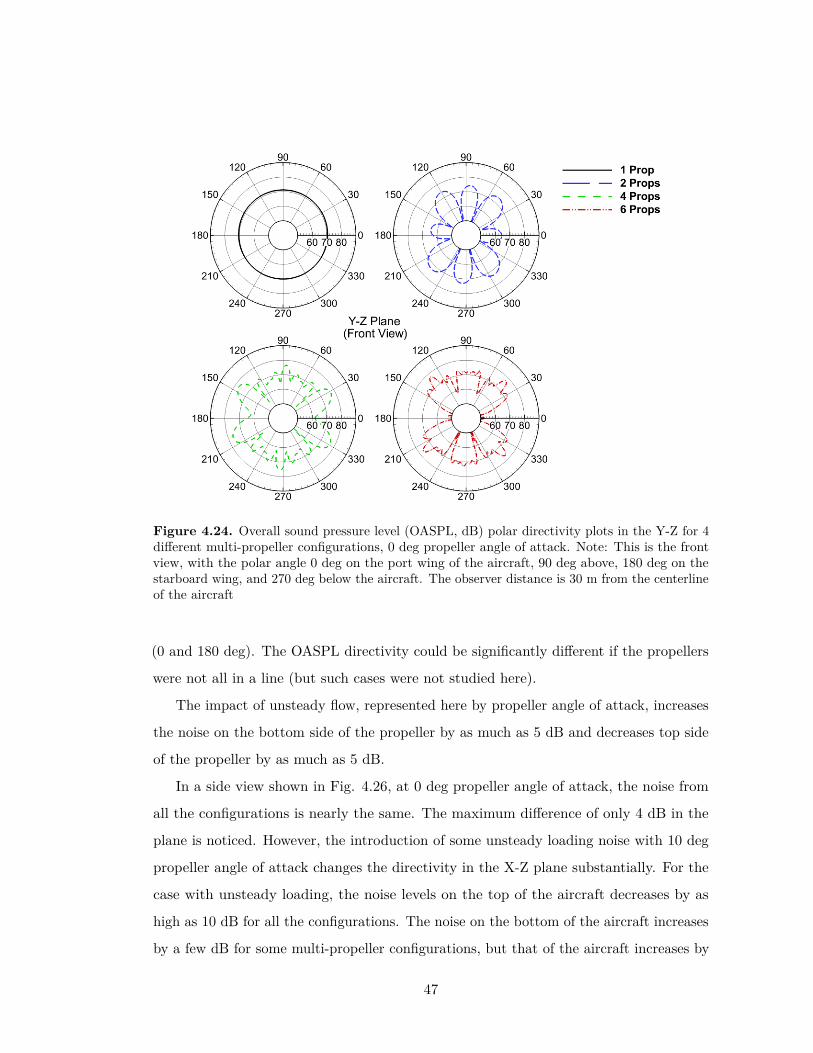
Figure 4.24. Overall sound pressure level (OASPL, dB) polar directivity plots in the Y-Z for 4di�erent multi-propeller configurations, 0 deg propeller angle of attack. Note: This is the frontview, with the polar angle 0 deg on the port wing of the aircraft, 90 deg above, 180 deg on thestarboard wing, and 270 deg below the aircraft. The observer distance is 30 m from the centerlineof the aircraft

(0 and 180 deg). The OASPL directivity could be significantly di�erent if the propellers

were not all in a line (but such cases were not studied here).

The impact of unsteady flow, represented here by propeller angle of attack, increases

the noise on the bottom side of the propeller by as much as 5 dB and decreases top side

of the propeller by as much as 5 dB.

In a side view shown in Fig. 4.26, at 0 deg propeller angle of attack, the noise from

all the configurations is nearly the same. The maximum di�erence of only 4 dB in the

plane is noticed. However, the introduction of some unsteady loading noise with 10 deg

propeller angle of attack changes the directivity in the X-Z plane substantially. For the

case with unsteady loading, the noise levels on the top of the aircraft decreases by as

high as 10 dB for all the configurations. The noise on the bottom of the aircraft increases

by a few dB for some multi-propeller configurations, but that of the aircraft increases by

47

Figure 4.25. Multi-propeller overall sound pressure level (OASPL, dB) polar directivity inY-Z plane (front view) for two di�erent propeller angles of attack (0 and 10 deg). The observerdistance is 30 m from the centerline of the aircraft.

Figure 4.26. Multi-propeller overall sound pressure level (OASPL, dB) polar directivity in X-Zplane (side view) for three di�erent propeller angles of attack (0 and 10 deg). The observerdistance is 30 m from the centerline of the aircraft.

as high as 5 dB for the single-propeller configuration.

48

Table 4.5. Input parameters of CROTOR for 1-propeller configuration operating at Mtip=0.4

Table 4.6. Input parameters of CROTOR for 4-propeller configuration operating at Mtip=0.4

Table 4.7. Input parameters of CROTOR for 6-propeller configuration operating at Mtip=0.4

49

Chapter 5 |Concluding Remarks

5.1 Conclusions

The noise of a single propeller of similar size and capability as that used by the Tecnam

P2012, but designed by CROTOR at Mtip = 0.7, has been compared to the noise of

single propellers designed to operate at lower tip speeds (also designed by CROTOR).

For all the comparisons, the propeller/aircraft forward speed was fixed and the thrust

was held constant (either the same per propeller when comparing isolated propellers or

total thrust fixed for multi-propeller configurations).

In general, the noise is reduced dramatically by reducing the tip speed, but this noise

reduction below the propeller at a high angle of attack is diminished by a significant

amount due to an increase in noise associated with unsteady loading (modeled as a

propeller at an angle of attack in this work).

The unsteady loading is even more important at lower tip speeds because the thickness

noise tends to decrease more rapidly with tip Mach number than the loading noise. The

contribution of thickness noise of a propeller designed for Mtip = 0.3 is minimal where

the total noise distribution is almost the same as the loading noise distribution. Due to

the unsteady loading at high angle of attack of 10 deg, the noise distribution below the

propeller always tends to increase by as high as 6 dB and shifts its directivity by the angle

of attack. Since the propeller noise on the bottom is radiating towards the communities,

the e�ect of unsteady loading should be investigated more in depth. Although the noise

50

of propellers designed at Mtip = 0.3 are lower than that of propellers designed at Mtip =

0.4 and 0.7 in general, low tip speed designs could have higher noise at some elevation

angles due to unsteady loading. Interestingly, the noise in plane of 6-bladed propellers

has a linear relationship with tip speed. (Mtip = 0.3 ≠ 0.7)

Increasing the number of blades, for a fixed propeller thrust, tends to decrease

the OASPL levels, but the rate of decrease with increase in number of blades is more

pronounced in the propeller plane.

For multi-propeller configurations operating at Mtip = 0.4 rotational tip-Mach number,

the directivity pattern in the plane of the propellers becomes more complex when more

propellers are used and the direction in which the noise is maximum can be impacted by

the number of propellers.

5.2 Recommendations for Future Work

In this section, recommendations are made on how to continue with this research and

what subjects can be investigated more in depth to make the study more robust. This

project was intended to investigate noise of electric, low-tip-speed propellers.

In 1974, Gri�th and Revell [20] found that noise predictions for a low tip speed

propeller were strongly dependent upon a complete accounting of unsteady loading and

broadband noise (angle of attack, yaw, and inflow disturbance, etc.) The noise was

significantly more accurate when the unsteady loading and broadband was included in

the noise predictions. In this research, CROTOR was used to produce approximate

quasi-steady loading for the propeller to calculate the unsteady loading calculation, and

the noise reduction in propeller noise was done by reducing tip-speed for both steady

and unsteady inflow cases. However, to make the prediction more accurate, broadband

noise should be included in the prediction process. The propeller noise prediction is never

complete without considering the broadband noise although its significance may be less

than the unsteady loading noise as shown in Gri�th and Revell’s work [20].

It was also concluded in this thesis that increasing the number of blades results in a

reduction in propeller noise. Having propellers with higher number of blades might not

51

always result in a reduction in noise because broadband noise, which is not considered

in this research, may contribute a significant part of total noise for propellers with high

number of blades, especially for low-tip-speed propellers. This should be investigated

more thoroughly for low-tip-speed propellers, especially at di�erent sizes (UAV scale vs

manned aircraft scale).

It was seen that multiple propeller configurations, such as the 6-propeller configuration,

generate less noise than a conventional two propeller configuration for a steady inflow

case. In the steady inflow case, the noise of 6-propeller configurations is still less than

2-propeller configuration in some directions. However, considering broadband noise in

the total noise may result in di�erent conclusions because interaction between propellers

can be very complicated, especially for high number of propeller configurations.

Finally, the noise cancellation techniques applying destructive interference on acoustic

pressure signals from the propellers are recommended to be investigated. In some cases,

the destructive interference between thickness and loading noise signals can be seen in

propeller noise. For that reason, the phasing angle, rotational direction, and spacing of

the propellers are important parameters in propeller noise that could allow designers to

alleviate the propeller noise.

52

References

[1] Swift, Hales, “Potential Health E�ects of Aircraft Noise,” Final Report 19, PurdueUniversity, July 2010.

[2] Berglund, B., Lindvall, T., Schwela, D.H. “Community Noise,” Archives of the Centrefor Sensory Research, Vol. 2, Issue 1, Stockholm University and Karolinska Institute,1995.

[3] Danzon et al. “Night Noise Guidelines For Europe,” World Health Organizations,2009.

[4] Ackerman, E., “NASA’s LEAPTech X-plane Will Fly with 18 Electric Motorsand Tiny Wings” Last retrieved March 19, 2015, https://spectrum.ieee.org/tech-talk/aerospace/aviation/nasas-newest-xplane-will-fly-with-18-electric-motors.

[5] Uber, “Uber Elevate: Fast-Forwarding to a Future of On-Demand Urban Air Trans-portation,” Uber, 2016 https://www.uber.com/elevate.pdf.

[6] Stewart, J.,“Airbus’ Vahana Makes Its First Flight,” Retrieved fromhttps://www.wired.com/story/airbus-vahana-first-flight-faa-certification-flying-cars/ February 2018.

[7] German, B.,“Economical Thin-Haul Aviation Operation Study,” Annual Report,School of Aerospace Engineering, Georgia Tech, 2016.

[8] Lighthill, M. J. “On sound generated aerodynamically. I: General Theory,” Proc RSoc A 1952;211:564-87.

[9] Ffowcs Williams, J.E., Hawkings, D.L., “Sound generated by turbulence and surfacesin arbitrary motion,” Philos. Trans. R. Soc. A 1969; 264(1151):321-42

[10] Farassat, F. and Succi, G. P., “The Prediction of Helicopter Discrete FrequencyNoise,” Vertica, 7(4):309-320, 1983.

[11] Leishman, J. G., “Principles of Helicopter Aerodynamics,” Cambridge UniversityPress, 2010.

[12] Carter, P., “CROTOR - XROTOR on Steroids” Last retrieved December 13, 2017,http://www.esotec.org/sw/crotor.html.

53

[13] Larrabee, E. E., French, S. E., “Minimum induced loss windmills and propellers,”Journal of Wind Engineering and Industrial Aerodynamics, Volume 15, Issues 1-3,December 1983, Pages 317-327.

[14] Kuijk, J., J., A. V., “Analysis of Swirl Recovery Vanes,” MS thesis. TechnischeUniversiteit Delft, Netherlands, 2015.

[15] Larrabee, E. E., “Five Years Experience with Minimum Induced Loss Propellers,”Journal Article, SAE International, Vol. 93, Section 1: 840002–840220 (1984), pp.1130-1137, Netherlands, 2015.

[16] Brentner, K. S., “Challenges of Extremely Quiet Propulsion,” Presentation, Sustain-able Aviation Symposium, San-Francisco, California, 2018.

[17] Brés, G. A., Brentner, K. S., Perez, G., and Jones, H. E., “Maneuvering rotorcraftnoise prediction,” Journal of Sound and Vibration, 275(3-5):719-738, August 2004.

[18] Brés, G. A., “Modeling the noise of arbitrary maneuvering rotorcraft: Analysisand implementation of the PSU-WOPWOP noise prediction code,” M.S. thesis,Department of Aerospace Engineering, The Pennsylvania State University, June2002.

[19] Perez, G., “Investigation of the influence of maneuver on rotorcraft noise,” M.S.thesis, Department of Aerospace Engineering, The Pennsylvania State University,June 2002.

[20] Gri�th, E. D. Revell, J., “Low Noise Propeller Technology Demonstration,” ReportAD-779 773 (AFAPL-TR-73-115), Lockheed California Company, 1974.

[21] Hicks, C. W. Hubbard, H. H, “Comparison of Sound Emission from Two-Blade,Four-Blade, AND Seven-Blade Propellers,” NACA-Technical Note, Washington, 1947.

[22] Torenbeek, Egbert, “Synthesis of Subsonic Airplane Design: An introduction to thepreliminary design of subsonic general aviation and transport aircraft, with emphasison layout, aerodynamic design, propulsion and performance,” Springer Netherlands,1982.

[23] Hreinsson, G. S., “Aircraft Noise,” Virginia Polytechnic Institute and State University,Blacksburg, VA, December 1993.

[24] Chen, H., Brentner, K. S., Lopes, L. V., and Horn, J. F., “A Study of RotorcraftNoise Prediction in Maneuvering Flight,” Proceedings of 42nd AIAA AerospaceSciences Meeting and Exhibit, Reno, NV, January 5-8 2004.

[25] Chen, H., Brentner, K., L.V., L., and Horn, J., “An Initial Analysis of TransientNoise in Rotorcraft Maneuvering Flight,” International Journal of Aeroacoustics,Vol. 5, No. 1, 2006, pp. 1-30.

[26] Munch, C. L., “Prediction of V/STOL Noise for Applications to Community NoiseExposure,” Technical Report TSC-OST-73-19, DOT, May 1973

54

[27] Kalki, S., “Incorporating acoustic assessment into the design and analysis of rotor-craft,” M.S. thesis, Department of Aerospace Engineering, The Pennsylvania StateUniversity, December 2016.

[28] Brooks, T. F., Burley, C. L., “Rotor Broadband Noise Prediction with Comparisonto Model Data,” Journal of the American Helicopter Society, 49:1 (January 2004).

[29] Shirey, J. S., Brentner, K. S., and Chen, H., “A Validation of the PSU-WOPWOPRotor Noise Prediction System,” 45th Aerospace Sciences Meeting and Exhibit,Reno, Nevada, January 8-11, 2007.

[30] Brentner, K. S., Farassat, F., “Modeling aerodynamically generated sound of heli-copter rotors,” Progress in Aerospace Sciences 2003;39:83-120.

[31] Wachspress, D. A., Brentner, K. S., and Page, J. A., “Real-Time Noise Predictionof V/STOL Aircraft in Maneuvering Flight,” CDI Report No. 05-14 under NASAContract NNL05AB01P, July 2005.

[32] Brentner, K. S., Zolbayar, B., and Jaworski, F., J.,“Investigation of Noise FromElectric, Low-Tip-Speed Aircraft Propellers,” AHS Specialists’ Conference, SanFrancisco, CA, January, 2018.

55