Embed Size (px)
Citation preview
Investigation of Advanced Modulation and Multiplexing
Schemes for High-Capacity Optical Transmission Systems
by
An Li
Submitted in total fulfilment of
The requirements of the degree of
Doctor of Philosophy
Department of Electrical and Electronic Engineering
The University of Melbourne
VIC 3010, Melbourne, Australia
July 2012
Printed on archival quality paper.

Copyright © AN LI
All rights reserved. No part of the publication may be reproduced in any form by print,
photoprint, microfilm or any other means without written permission from the author.
i
Abstract
Investigation of Advanced Modulation and Multiplexing
Schemes for High-Capacity Optical Transmission Systems
by An Li
Space-division multiplexed (SDM) transmission based on multi-core (MCF) or multi-
mode fibre (MMF) emerges as one of the promising solutions for overcoming the
capacity limit of standard single mode fibre (SSMF). However, to unleash the full
potential of the high data rate SDM transmission, brand-new research on the device to
system level is required. In this thesis, we elucidate the overall system architecture,
critical components and sub-system modules for mode-division multiplexed (MDM)
transmission and report our latest demonstration of MDM superchannel transmission
based on few-mode fibre (FMF). We envisage that the combination of MDM and
OFDM modulation could provide a viable pathway to the future Tb/s and beyond
optical transports.
We first review the basic concepts and principles of conventional optical OFDM
system. We introduce two novel variants of coherent optical OFDM (CO-OFDM)
system, namely the wavelet packet transform based OFDM (WPT-OFDM) and
discrete Fourier transform based OFDM (DFTS-OFDM). The performance of the two
new systems are analysed and compared with conventional CO-OFDM system. We
next look at the most basic but important element for the SDM transmission system –
FMF few-mode fibre (FMF).We then show an experimental demonstration of
characterization of physical property of a custom-designed TMF fibre. After that we
investigate a broad range of issues on SDM -especially the MDM based on MMF or
FMF - from its fundamentals to some of the critical FMF components including mode
stripper, mode converter, mode combiner and few-mode amplifiers. With these few-
mode components and subsystem module available, we then show experimental
demonstrations of MDM transmission over TMF fibre under three different unique
MDM schemes:(1) LP01/LP11 mode, (2) dual-LP11 mode, and (3) triple-mode
(LP01+LP11a+LP11b). Finally, the research outcome in this thesis is summarized and a
few research directions toward future work are presented.

ii
This is to certify that
(i) the thesis comprises only my original work,
(ii) due acknowledgement has been made in the text to all other material used,
(iii) the thesis is less than 100,000 words in length, exclusive of table, maps,
bibliographies, appendices and footnotes.
Signature______________________
Date__________________________

iii
Declaration
I hereby declare that this thesis comprises only my original work. No material in this
thesis has been previously published and written by another person, except where due
reference is made in the text of the thesis. I further declare that this thesis contains no
material which has been submitted for a degree or diploma or other qualifications at
any other university. Finally, I declare that the thesis is less than 100,000 words in
length, exclusive of tables, figures, bibliographies, appendices and footnotes.
iv
Acknowledgements
Although this thesis consists of academic achievements as a summarization of my
PhD study, more precisely it is teamwork from everyone who has ever helped me
including my supervisors, collaborators, friends and also my family. The work cannot
be fulfilled without their great support.
First I would like to express my sincere gratitude to my supervisor, Prof. William
Shieh and co-supervisor Prof. Rod Tucker, for their patient supervision and advice
throughout my entire PhD candidature. Their high- quality academic guidance and
meticulous attention to detail helped me develop my skills quickly and lead me to the
cutting-edge research topics. In addition, I would also like to express my thanks to Dr.
Fred Buchali at Bell labs, Alcatel-Lucent Germany for providing me an invaluable
opportunity to undertake an internship, where I have learned a lot from you and other
experts in Bell labs. It is such a wonderful time that I will never forget in my life.
My second thanks are given to the other members in Prof. William Shieh's group.
Xi Chen, Guanjun Gao, Simin Chen and Abdullah Al Amin, my best research partners
and friends I have ever had. I never get bored when I was doing experiment in the lab
as long as they are around. We are the best team together to have so many OFC
postdeadline papers for years. Without their contribution, I could never win the award
of Corning's Outstanding Student Paper in OFC 2012. The other newly joined
members - Jia Ye, Jiayuan He, and Qian Hu, have also helped me a lot during my
thesis writing.
I am also grateful to The University of Melbourne and Department of Electrical &
Electronic Engineering for providing me the MIFRS and MIRS scholarships, as well
as friendly study environment and facilities. Furthermore, I am grateful to the Centre
for Energy Efficient Telecommunications (CEET) for providing me the PhD top-up
scholarship for the last year of my study.
Last but not least, I would like to give my special thanks to my dearest parents and
sister. You are my spiritual strength and anchor when I am abroad. I love you from
the deepest of my heart! There are many people who have helped me but I forget to
mention here, thank you so much and wish you all the best for the future!

v
Contents
ABSTRACT .................................................................................................................. I
DECLARATION ....................................................................................................... III
ACKNOWLEDGEMENTS ..................................................................................... IV
CONTENTS ................................................................................................................. V
LIST OF FIGURES ............................................................................................... VIII
LIST OF TABLES ..................................................................................................XIV
1 INTRODUCTION ................................................................................................ 1
1.1 OVERVIEW ...................................................................................................... 1
1.1.1 Optical communications and fibre optics .................................................. 1
1.1.2 High speed optical communication systems .............................................. 2
1.2 MOTIVATION ................................................................................................... 3
1.3 THESIS OUTLINE .............................................................................................. 4
1.4 CONTRIBUTIONS ............................................................................................. 7
1.5 PUBLICATIONS RELATED TO THIS THESIS ......................................................... 7
2 LITERATURE REVIEW ................................................................................. 11
2.1 INTRODUCTION ............................................................................................. 11
2.2 ADVANCED MULTIPLEXING SCHEMES FOR HIGH-CAPACITY OPTICAL
TRANSMISSION .......................................................................................................... 11
2.2.1 WDM transmission systems ..................................................................... 11
2.2.2 OTDM transmission systems.................................................................... 13
2.2.3 Coherent optical OFDM (CO-OFDM) .................................................... 16
2.2.4 Direct detection optical OFDM (DDO-OFDM) ...................................... 19
2.2.5 Variants of CO-OFDM transmission systems .......................................... 24
2.2.6 Space-division multiplexing (SDM) ......................................................... 26
3 PRINCIPLE OF OPTICAL OFDM SYSTEM ............................................... 30
3.1 PRINCIPLE OF OFDM SYSTEM ....................................................................... 30
3.2 PRINCIPLE OF CO-OFDM ............................................................................. 32
3.3 PMD SUPPORTED TRANSMISSION IN CO-OFDM SYSTEM ............................. 35
4 NOVEL VARIANTS OF COHERENT OPTICAL OFDM SYSTEM FOR
FUTURE HIGH-SPEED OPTICAL NETWORKS ............................................... 38
4.1 INTRODUCTION ............................................................................................. 38
4.2 WAVELET PACKET TRANSFORM BASED OFDM SYSTEM (WPT-OFDM) ....... 38
vi
4.2.1 Fourier transform (FT) and wavelet transform (WT) .............................. 38
4.2.2 Wavelet packet transform (WPT) ............................................................. 45
4.2.3 Commonly used wavelets ......................................................................... 49
4.2.4 System configuration of WPT-OFDM ...................................................... 51
4.2.5 Simulation and results .............................................................................. 55
4.3 DISCRETE FOURIER TRANSFORM SPREAD OFDM SYSTEM (DFTS-OFDM) .. 64
4.3.1 System configuration of DFTS-OFDM .................................................... 65
4.3.2 Principle of unique word DFTS-OFDM (UW-DFTS-OFDM) ................ 67
4.3.3 Simulation and Results ............................................................................. 69
4.3.4 Experimental demonstration of 1-Tb/s PDM-QPSK UW-DFTS-OFDM
superchannel transmission ................................................................................... 71
4.3.5 Experimental demonstration of 1.63-Tb/s PDM-16QAM UW-DFTS-
OFDM superchannel Transmission ..................................................................... 80
4.4 CONCLUSION ................................................................................................. 85
5 FEW-MODE AND TWO-MODE FIBRE ....................................................... 87
5.1 OVERVIEW OF OPTICAL FIBRES ...................................................................... 87
5.2 FUNDAMENTALS OF FIBRE MODES ................................................................. 89
5.3 FEW-MODE FIBRE FOR TERABIT AND BEYOND OPTICAL NETWORKS ............... 91
5.4 TWO-MODE FIBRE DESIGN ............................................................................. 91
5.5 FIBRE CHARACTERIZATION ........................................................................... 93
5.5.1 Physical properties .................................................................................. 93
5.5.2 Characterization of linear impairments ................................................... 95
5.6 CONCLUSION ................................................................................................. 97
6 FUNDAMENTALS OF SPACE-DIVISION MULTIPLEXING AND
DESIGN OF FEW-MODE COMPONENTS .......................................................... 98
6.1 ARCHITECTURE OF SDM BASED HIGH SPEED SUPERCHANNEL SYSTEM ......... 98
6.2 FEW-MODE COMPONENTS ............................................................................. 99
6.2.1 Mode stripper ........................................................................................... 99
6.2.2 Mode converter ...................................................................................... 100
6.2.3 Mode combiner ...................................................................................... 103
6.2.4 Few-mode fibre amplifier (EDFA, Raman) ........................................... 117
6.3 COMPARISON OF SDM TECHNIQUES ........................................................... 118
6.4 CONCLUSION ............................................................................................... 119
7 TRANSMISSION OF MODE-DIVISION-MULTIPLEXED CO-OFDM
(MDM-CO-OFDM) SIGNAL OVER TWO-MODE FIBRE ............................... 120
7.1 TRANSMISSION OF LP01/LP11 MODE MDM-CO-OFDM SIGNAL OVER TWO-
MODE FIBRE ............................................................................................................ 120
vii
7.1.1 System setup ........................................................................................... 120
7.1.2 Result and Discussion ............................................................................ 121
7.2 TRANSMISSION OF DUAL-LP11 MODE MDM-CO-OFDM SIGNAL OVER TWO-
MODE FIBRE ............................................................................................................ 124
7.2.1 System setup ........................................................................................... 124
7.2.2 Result and Discussion ............................................................................ 125
7.3 TRANSMISSION OF TRIPLE-MODE (LP01+LP11A+LP11B) MDM-CO-OFDM
SIGNAL OVER TWO-MODE FIBRE .............................................................................. 129
7.4 CONCLUSION ............................................................................................... 130
8 CONCLUSIONS .............................................................................................. 131
8.1 SUMMARY OF THIS WORK ............................................................................ 131
8.1.1 Novel variants of CO-OFDM system ..................................................... 131
8.1.2 Few-mode fibre and components for SDM ............................................ 131
8.1.3 Transmission of MDM-CO-OFDM over Two-mode fibre ..................... 131
8.2 FUTURE WORK AND PERSPECTIVES.............................................................. 132
BIBLIOGRAPHY .................................................................................................... 133
APPENDIX A ........................................................................................................... 153
ACRONYMS ............................................................................................................ 153
viii
List of Figures
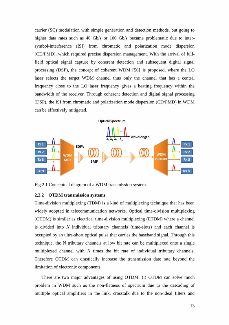
Fig.2.1 Conceptual diagram of a WDM transmission system. .................................... 13
Fig.2.2 Experimental setup of a 160-Gb/s OTDM transmission system with all-
channel independent modulation MUX and all-channel simultaneous DEMUX.
E-MUX: electrical MUX. CW: continuous-wave laser source. MOD: LiNbO3
intensity modulator. OBPF: optical bandpass filter. SMF: single-mode fibre.
RDF: reverse dispersion fibre. O/E: optoelectronic converter. E-DEMUX:
electrical DEMUX. .......................................................................................... 14
Fig.2.3 A CO-OFDM system in (a) direct up/down conversion architecture, and (b)
intermediate frequency (IF) architecture. ........................................................ 17
Fig.2.4 Coherent detection using an optical hybrid and balanced photo-detection. .... 17
Fig.2.5 Illustration of linearly-mapped DDO-OFDM (LM-DDO-OFDM) where the
optical OFDM spectrum is a replica of the baseband OFDM spectrum. ......... 20
Fig.2.6 Direct-detection optical OFDM (DDO-OFDM) long-haul optical
communication systems. After Ref. [71] ......................................................... 22
Fig.2.7 Comparison of optical spectra between (a) NLM-DDO-OFDM through direct-
modulation of DFB laser, and (b) externally modulated offset SSB DDO-
OFDM. The chirp constant C of 1 and the modulation index m of 0.3 are
assumed for direct-modulation in (a). Both OFDM spectrum bandwidths are 5
GHz comprising 256 subcarriers. .................................................................... 24
Fig.2.8 Schematic of a free-space 3×1 mode combiner using phase-plate based mode
converters [105]. .............................................................................................. 27
Fig.2.9. (a) Spot generation using mirrors with sharp edges. (b) Experimental setup of
the low-loss mode coupler. (c) Mode profile at the end facet of 154-km hybrid
FMF [109]. ....................................................................................................... 28
Fig.2.10 Schematic diagram of a LPFG based LP01/LP11 mode converter [98-102]. .. 28
Fig.3.1 Conceptual diagram for a generic multi-carrier modulation (MCM) system. . 30
Fig.3.2 OFDM symbol in time domain. ....................................................................... 32
Fig.3.3 Conceptual diagram of CO-OFDM system. S/P: Serial-to-parallel, GI: Guard
Interval, (I)DFT: (Inverse) Discrete Fourier Transform, LPF: Low Pass Filter,
MZM: Mach-Zehnder Modulator, PD: Photodiode. ........................................ 33
Fig.3.4 A variation of CO-MIMO-OFDM system: two-input two-output (TITO) [126].
.......................................................................................................................... 35
Fig.4.1 Time-Frequency representation of Fourier transform and wavelet transform. 39
Fig.4.2 Scaling function and wavelet vector spaces. ................................................... 41
Fig.4.3 Block diagram of a discrete wavelet transform (DWT) with 3 level filter banks.
↓2 stands for two times down-sampling. f(ti) at the input is the sampled input
signal f(t). ......................................................................................................... 44
Fig.4.4 Frequency domain responses of Discrete Fourier transform(DFT) and discrete
wavelet transform(DWT) (a) DFT with uniform division of bandwidth. (b)
DWT with dyadic division of bandwidth. ........................................................ 44
ix
Fig.4.5 Implementation of discrete wavelet packet transform (DWPT). ↓2 stands for
2 times down-sampling. ................................................................................... 48
Fig.4.6 Implementation of inverse discrete wavelet packet transform (IDWPT). ↑2
stands for 2 times up-sampling. ....................................................................... 48
Fig.4.7 Filter coefficients of Haar wavelet (a) low-pass filter (b) high-pass filter. ..... 49
Fig.4.8 Filter coefficients of db10 wavelet (a) low-pass filter (b) high-pass filter. ..... 50
Fig.4.9 Filter coefficients of coif5 wavelet (a) low-pass filter (b) high-pass filter. ..... 50
Fig.4.10 Filter coefficients of joh64(E) wavelet (a) low-pass filter (b) high-pass filter.
.......................................................................................................................... 51
Fig.4.11 Conceptual diagram of WP(F)T-OFDM system setup. For WPT-OFDM,
IDWPT and DWPT are used as a pair, and for FT-OFDM, IDFT and DFT are
used as a pair. PBC/PBS: Polarization Beam Combiner /Splitter, LPF: Low
Pass Filter. GI: Guard Interval, arbitrary length of CP can be inserted for FT-
OFDM but not available for WPT-OFDM ...................................................... 52
Fig.4.12 Time domain representation of 8 coif5 wavelet packets, constructed using 3-
level IDWPT. ................................................................................................... 53
Fig.4.13 Frequency domain representation (Spectrum) of 8 coif5 wavelet packets,
constructed using 3-level IDWPT. ................................................................... 53
Fig.4.14 A conceptual illustration of the PMD impact on k-th wavelet packet in WPT-
OFDM systems for x polarization component. ................................................ 54
Fig.4.15 Electrical spectrum of simulated 112 Gb/s dual-polarization WPT-OFDM
system using db32 wavelet. ............................................................................. 57
Fig.4.16 BER vs. transmission distance for WPT-OFDM and FT-OFDM. CD = 17
ps/nm/km. Wavelets are Haar, Coiflet, Daubechies [84] and Johnston [85]
family. Number of subcarriers Nsc = 64. ........................................................ 58
Fig.4.17 BER vs. OSNR for WPT-OFDM without DGD (0ps) and with DGD (10ps).
Nsc = 64. .......................................................................................................... 59
Fig.4.18 Required OSNR at BER=1×10⁻³
vs. DGD for WPT-OFDM. Nsc = 64........ 59
Fig.4.19 OSNR penalty vs. DGD for FT-OFDM without CP and with CP of 1/8. ..... 60
Fig.4.20 OSNR penalty vs. DGD for WPT-OFDM using Johnston wavelet with Nsc =
64, 128, 256. ..................................................................................................... 60
Fig.4.21 CCDF of PAPR for WPT-OFDM and FT-OFDM. Nsc = 64, oversampling
factor No = 1. ................................................................................................... 61
Fig.4.22 CCDF of PAPR for WPT-OFDM and FT-OFDM. Nsc = 64, No = 8. ......... 62
Fig.4.23 BER vs. launch power after 2×100 km transmission. CD in each span is fully
compensated by DCF. Nsc = 64, No = 8. ........................................................ 62
Fig.4.24 BER vs. launch power after 2×100 km transmission. CD in each span is 95%
compensated by DCF. ...................................................................................... 63
Fig.4.25 Signal processing of conventional OFDM and DFTS-OFDM. The pink
blocks show the additional pair of DFT/IDFT in DFTS-OFDM. .................... 65
x
Fig.4.26 Structure of UW-DFTS-OFDM data symbol. UW: Unique Word; CP: Cyclic
Prefix. ............................................................................................................... 68
Fig.4.27 Simulated Q factor as a function of launch power at transmission distance of
960-km for 1-Tb/s PDM-QPSK UW-DFTS-OFDM and conventional OFDM.
DFTS: DFTS-OFDM, Conv.: Conventional OFDM, Uni.: uniform filling,
Rand.: random filling. ...................................................................................... 70
Fig.4.28 Simulated Q factor as a function of launch power at transmission distance of
960-km for 1.63-Tb/s PDM-16QAM UW-DFTS-OFDM and conventional
OFDM. DFTS: DFTS-OFDM, Conv.: Conventional OFDM, Uni.: uniform
filling, Rand.: random filling. .......................................................................... 71
Fig.4.29 Experimental setup of 1-Tb/s UW-DFTS-OFDM system. OBPF: optical
band-pass filter; AWG: arbitrary waveform generator; PMF: polarization
maintaining fibre; PBC/PBS: polarization beam combiner/splitter; SSMF:
standard single mode fibre; SW: (optical) switch; WSS: wavelength selective
switch; LO: local oscillator; BR: balanced receiver; ADC: analogue-to-digital
converter. Insets: measured optical and electrical spectra of (i) 48-tone source;
(ii) data pattern loaded onto AWG; (iii) transmitted OFDM signal; (iv)
received OFDM signal. .................................................................................... 72
Fig.4.30 Digital signal processing at the transmitter and receiver of DFTS-OFDM.
Pilot symbols of the same pattern are inserted for timing synchronization and
frequency offset estimation using Schmidl-Cox's method [151]. For channel
estimation, a novel algorithm with hybrid short- and long- training sequences
is used. For phase noise compensation, a joint 'phase propagation' method that
combines DAML [152-153] and block-based DFML method [154] is used. .. 73
Fig.4.31 Structure of UW-DFTS-OFDM consisting of training and data symbol. UW:
Unique Word; CP: Cyclic Prefix. The bottom figure shows a realistic data
pattern generated and loaded onto the AWG in experiment. ........................... 75
Fig.4.32 Flow chart of channel estimation algorithm using hybrid short- and long-
training symbols. .............................................................................................. 76
Fig.4.33 Conceptual diagram of the proposed phase propagation method. The joint
method combines DAML method for the inter-block phase estimation and
block-based DFML method for the intra-block phase estimation with a block
size L. with a block size L. ............................................................................... 78
Fig.4.34 Measured optical back-to-back BER performance. The data rates shown are
raw data rates. DFTS: DFTS-OFDM; Conv.: conventional OFDM. ............... 79
Fig.4.35 Measured Q-factor vs. launch power after 8000-km transmission. Inset:
recovered constellations at the launch power of 9 dBm. ................................. 79
Fig.4.36 Measured BER performance of 1.0-Tb/s UW-DFTS-OFDM system at
different transmission distances. ...................................................................... 80
Fig.4.37 Measured BER performance for all 48 bands for 8,000-km transmission at a
launch power of 9 dBm. ................................................................................... 80
Fig.4.38 Experimental setup of 1.63-Tb/s PDM-16QAM UW-DFT-S-OFDM system.
PC: polarization controller; AWG: arbitrary waveform generator; PMF:
polarization maintaining fibre; PBC(S): polarization beam combiner(splitter);
SW: optical switch; WSS: wavelength selective switch; LO: local oscillator;
xi
BR: balanced receiver. DFT-S: DFT-S-OFDM; Conv.: conventional OFDM.
Insets: measured optical and electrical spectra of (i) 48-tone source; (ii)
Frequency domain data pattern loaded onto AWG; (iii) transmitted OFDM
signal; (iv) received OFDM signal. ................................................................. 81
Fig.4.39 Measured optical back-to-back BER performance of the center band. The
inset shows the recovered constellations at OSNR = 41 dB. DFT-S: DFT-S-
OFDM; Conv.: conventional OFDM. .............................................................. 84
Fig.4.40 Measured Q-factor vs. launch power. Inset: recovered constellations at the
launch power of 8 dBm. ................................................................................... 84
Fig.4.41 Measured Q-factor for the worst band of 1.6Tb/s PDM-16QAM-OFDM
system at different transmission distances. ...................................................... 85
Fig.4.42 Measured Q-factor for all 48 bands at the launch power of 8 dBm after
1,010-km transmission. .................................................................................... 85
Fig.5.1 Effective modal indices for the LP01 and LP11 modes of the custom-designed
TMF. The inset at the top right shows the step-index profile of the TMF [99].
.......................................................................................................................... 92
Fig.5.2 Measured refractive index profile of the custom-designed two-mode fibre [99].
.......................................................................................................................... 94
Fig.5.3 (a) Experimental setup for the measurement of mode profile. (b)-(e):
Measured mode profile of the custom-designed two-mode fibre [99]. (b) LP01
mode, (c) LP11a mode, (d) LP11b mode and (e) LP11a+LP11b mode. ................. 94
Fig.5.4 (a) Experimental setup for the measurement of DMD between LP01 and LP11
modes through coherent beating. (b) Optical spectrum before (black line) and
after (green line) a 1-m-long TMF fibre measured with an OSA. The spectral
power before TMF was scaled to be in the same region as after TMF and does
not reflect the real power level. ........................................................................ 96
Fig.6.1 Conceptual diagram of FMF based SDM superchannel transmission utilizing
few-mode compatible ROADM. ...................................................................... 98
Fig.6.2 Architecture of N×N SDM based superchannel transmission utilizing coherent
MIMO digital signal processing. MUX/DEMUX: multiplexer/demultiplexer,
Co-Rx: coherent receiver. ................................................................................ 99
Fig.6.3 Schematic diagram of a LPFG based LP01/LP11 mode converter. The groove
pitch Λ and pressure can be adjusted for optimization for certain wavelength
or conversion ratio. The deformation of fibre core is assumed to be s-bend arc
shape with radius r. ........................................................................................ 101
Fig.6.4 Simulated coupling efficiency (LP01 to LP11) versus effective coupling length
for a LPFG-based mode converter under the grating pitch Λ = 524 μm, at
wavelength of λ = 1550 nm. The three curves correspond to the core
deformation radius of r = 0.08, 0.1 and 0.2 μm, respectively. ..................... 102
Fig.6.5 Coupling efficiency (LP01 to LP11) versus wavelength for a LPFG-based mode
converter with core deformation r = 0.2 μm. Sim.: Simulation; Exp.:
Experiment. .................................................................................................... 102
Fig.6.6 Extinction ratio versus wavelength for a LPFG-based mode converter with
core deformation r = 0.2 μm. Sim.: Simulation; Exp.: Experiment. .............. 102
xii
Fig.6.7 Lab demonstration (side view) of a LPFG based LP01/LP11 mode converter.
........................................................................................................................ 103
Fig.6.8 Block diagram of a coherent MIMO system over a two-mode fibre (TMF).
Middle inset shows three possible spatial orientations: LP01, LP11a and LP11b.
PBC/PBS: polarization beam combiner/splitter. MUX/DEMUX:
multiplexer/de-multiplexer. ........................................................................... 104
Fig.6.9 Schematic diagram of a free-space mode combiner. BS: beamsplitter. The
precision stages have freedom of two-axes (X and Y. Z is the light propagation
axis). The beams are collimated before entering the BS to minimize the
divergence and distortion. .............................................................................. 105
Fig.6.10 Lab demonstration (top view) of a free-space mode combiner. .................. 106
Fig.6.11 (a) Mode selective combiner consisting of cascaded LP11 mode combiners.
c(e)-TMF: circular(elliptical)-core TMF. (b) coupler-1, couples LP01 mode of
SMFa to LP11a mode of e-TMF; (c) coupler-2, couples LP01 mode of SMFb
into LP11b mode of e-TMF. ............................................................................ 108
Fig.6.12 Fibre core geometry and eigen modes in an e-TMF. ................................... 109
Fig.6.13 Modal index as a function of wavelength for TE modes in an e-TMF. ...... 109
Fig.6.14 Normalized power coupled into LP11ax mode (target mode) as a function of
coupling length for coupler-1. ........................................................................ 111
Fig.6.15 Total power coupled into other modes: LP01x, LP01y, LP11ay, LP11bx, and
LP11by as a function of coupling length for coupler-1. .................................. 111
Fig.6.16 Normalized power coupled into LP11ay mode as a function of coupling length
for coupler-2. .................................................................................................. 112
Fig.6.17 Total power coupled into other modes: LP01x, LP01y, LP11ax, LP11ay, and
LP11bx as a function of coupling length for coupler-2. .................................. 112
Fig.6.18 Extinction Ratio of power coupled to LP11ax mode as function of coupling
length for coupler-1. At the first maximum (L = 3 mm) the extinction ratio is
above 21dB. ................................................................................................... 113
Fig.6.19 Extinction Ratio of power coupled to LP11bx mode as function of coupling
length for coupler-2. At the first maximum (L = 3 mm) the extinction ratio is
above 20 dB. .................................................................................................. 113
Fig.6.20 Coupling efficiency versus wavelength for both coupler-1 and -2, at coupling
lengths of 3 and 9 mm. ................................................................................... 115
Fig.6.21 Extinction ratio versus wavelength for both coupler-1 and -2, at coupling
lengths of 3 and 9 mm. ................................................................................... 115
Fig.6.22 Coupling efficiency as function of coupling length for various core
separation distances of 12, 15 and 18 μm. ..................................................... 116
Fig.6.23 Maximum coupling efficiency as function of core separation for both
couplers. ......................................................................................................... 116
Fig.6.24 Schematic diagram of a MM-EDFA [107]. ................................................. 117
Fig.7.1 Experimental setup for 107-Gb/s dual-mode dual polarization transmission
over 4.5-km TMF fibre. 'X' indicates controlled coupling between LP01 modes
xiii
of SMF and TMF by centre splicing. PBC: polarization beam combiner, MS:
mode stripper, MC: mode converter, PD: photodiode. .................................. 121
Fig.7.2 (a) Optical spectrum and (c) constellations of LP01 mode; (b) optical
spectrum, and (d) constellations for LP11 mode after 4.5-km transmission in 3
bands. ............................................................................................................. 123
Fig.7.3 Experimental setup of a coherent 4×4-MIMO system over a two-mode fibre
(TMF). PBC/PBS: polarization beam combiner /splitter. MC: mode converter,
MS: mode stripper. WSS: wavelength selective switch, emulated by a Finisar
waveshaper. .................................................................................................... 125
Fig.7.4 Measured channel matrix parameters for the two LP11 modes after 4.5-km
TMF transmission.(a) Real and imaginary components, and (b) phase of the
4×4 fibre channel matrix. The subcarrier indices are mapped from low to high
frequency. The subcarrier index difference of 1 corresponds to frequency
spacing of 78 MHz. ........................................................................................ 128
Fig.7.5 Received RF spectrum of one of the four tributaries after 4.5-km TMF
transmission. The 5-GHz guard band is intentionally made to avoid
intermixing product of signal in heterodyning. .............................................. 129
Fig.7.6 (a) Measured OSNR vs. BER performance for 8-QAM 4×4 MIMO-OFDM
system for back-to-back (B2B) and 4.5-km TMF transmission configuration.
(b) Constellation of received signal after 4.5-km TMF transmission with
OSNR = 19 dB. .............................................................................................. 129

xiv
List of Tables
Table 4.1 Simulation Parameters ................................................................................. 56
Table 5.1. Custom-designed step-index two-mode fibre[99-103] ............................... 92
Table 5.2. OFS-designed graded-index two-mode fibre[111]. Red italic values are
calculated from index profile. Black non-italic values are measurements. ..... 93
Table 6.1. Comparison of different SDM approaches (Information from [29-37, 98-
119, 171-185]) ................................................................................................ 118
Table 7.1. Measured performance of the mode demultiplexer .................................. 122
Table 7.2. Measured Q factor (in dB) 'Pol-x/y' stands for x/y polarization. .............. 123
Table 7.3. End-to-end loss of the experimental setup ................................................ 127
1
1 Introduction
1.1 Overview
1.1.1 Optical communications and fibre optics
There is a long history of using light for communication ever since the ancient time.
Similar to any other forms of telecommunication systems, an optical communication
system consists of a transmitter that encodes data and modulates them onto an optical
signal, a channel (optical fibre or air) which carries the optical signal to the
destination, and a receiver which detects and recovers the data from the received
optical signal. The prototype of modern optical communication systems can be traced
back to 1880 when Alexander Graham Bell invented his 'Photophone', which
transmitted a voice signal on a beam of light [1]. The obstacle to Bell's further
research is that many things such as fog or raindrops could interfere with the
Photophone. Even then, scientists had been in the long seeking for the best material
for light communications until the introduction of fibre optics, a contained
transmission of light through long optical fibres. Although there were uncladded glass
fibres fabricated earlier in the 1920s [2]–[4], the field of fibre optics was not born
until the 1950s when the use of a cladding layer led to considerable improvement in
the fibre characteristics [5]-[8]. Since 1960s the field of fibre optics has been well-
developed. However, the early fibres (such as bundle of glass fibres) were very lossy
(>1000 dB/km) compared to modern telecommunication fibres. This situation
changed in 1970 followed an earlier Nobel Prize work and suggestion by K. C. Kao in
[9] that the losses of silica fibre span be reduced to below 20 dB/km. The progress in
fibre fabrication technology [10] in 1979 results in a loss of as low as 0.2 dB/km in
the 1.55 µm wavelength window [11], which has been standardized as the C-band in
modern telecommunication systems. Typically optical fibres consist of a transparent
core surrounded by a transparent cladding material with a lower index of refraction.
This makes fibre a waveguide where light is kept in the core by total internal
reflection [12].
Although there are other types of channels used such as air in free-space optical
communication (FSO) [13], optical fibre is the most commonly used channel in
modern optical communication systems. The advantage of using optical fibres,
compared with metal media such as copper wires, is that silica fibres can transmit
2
infrared optical signals with small attenuation over long distance, and are also
immune to electromagnetic interference.
1.1.2 High speed optical communication systems
Since the arrival of internet in early 1980, the data traffic growth on the internet has
lead to a higher and higher data transmission speeds over optical fibre networks from
1-Gb/s, to 10-Gb/s, to today's 100-Gb/s. The internet has been continuously growing
and in order to satisfy the demand on the capacity, intensive study has been made on
the long-haul high-capacity optical communication systems. The backbone and
metropolitan area network (MAN) should be scaled up accordingly in anticipation of
the upsurge of the traffic. Nowadays, single-channel data transmission rate over 100-
Gb/s has become a commercial reality, thanks to re-emergence of coherent detection
technologies in combination with high-speed electronic digital-to-analogue and
analogue-to-digital converter (DAC/ADC) and digital signal processing (DSP).
Together with wavelength-division multiplexing (WDM), polarization-division
multiplexing (PDM) and high order modulation schemes, the highest reported single
optical fibre data transmission capacity has reached over 100-Tb/s [14]-[15].
State-of-the-art digital communication systems can be grouped into two categories,
single-carrier modulation (SCM) and multi-carrier modulation (MCM). For SCM
systems, as the name suggests, the data is carried with a single optical carrier, which
has been the dominant modulation format for optical communications over three
decades. However, with the increase of network data rate and reach, the optical signal
is extremely sensitive to the chromatic dispersion (CD), polarization mode dispersion
(PMD), reconfigurable optical add/drop multiplexer (ROADM) filtering effects, and
imperfections of the electric-optics components. These place significant challenges on
the conventional SCM system. For MCM systems, the data is divided and carried by a
large number of low symbol rate carriers (called sub-carriers). Orthogonal frequency-
division multiplexing (OFDM) is a frequency-division multiplexing (FDM) scheme
by which a large number of closely-spaced orthogonal subcarriers are used to carry
data. With OFDM, each sub-carrier is modulated with a conventional modulation
scheme (such as quadrature amplitude modulation or phase-shift keying) at a low
symbol rate, maintaining total data rates similar to conventional single-carrier
modulation schemes in the same bandwidth. OFDM has been adopted for broad range
of applications in wideband digital communications, wireless or over copper wires,
3
such as digital television and audio broadcasting, wireless networking and broadband
internet access [16]. In fibre-optic communications, optical orthogonal frequency
division multiplexing (O-OFDM) has recently attracted many interests from the
optical communication community [17-18] because of its high spectral efficiency and
robustness against impairments such as CD and PMD. Direct-detection optical OFDM
(DDO-OFDM) was first proposed with a simple architecture and has been actively
pursued by several groups [17, 19-23]. Coherent optical OFDM (CO-OFDM) was
also proposed with coherent detection, which shows benefits of high spectral
efficiency (SE) and high receiver sensitivity [18]. The advantage of CO-OFDM is
prominent. It has the highest performance in receiver sensitivity, SE and robustness
against linear channel impairments. By appropriately choosing the length of cyclic
prefix (CP) and insert training symbols at the transmitter, both inline CD and PMD
can be fully compensated via digital signal processing (DSP). However, the
disadvantages of CO-OFDM also cannot be ignored. It requires a local oscillator (LO)
at the receiver, and is more sensitive to phase noise. CO-OFDM receiver also needs
two pairs of balanced receivers therefore it is more costly and complex than DDO-
OFDM. In addition, CO-OFDM also suffers from high peak-to-average-power ratio
(PAPR) that leads to inferior nonlinearity tolerance than single-carrier system.
1.2 Motivation
The highest reported single optical fibre data transmission speed has reached over 100
Tb/s [14]-[15]. However, there is a need to continue enhancing the total data
transmission capacity while keeping the signals within the available optical spectrum
of the conventional Erbium doped fibre amplifier (EDFA), which translates into the
requirement for increased SE (expressed in b/s/Hz). Although Shannon's theory
predicts SE to increase with higher received SNR as a result of increased transmission
power, fibre nonlinearity imposes a hard limit on improving channel capacity [24].
We intend to explore various modulation and multiplexing schemes to improve
the transmission performance. First we study two new variants of the CO-OFDM
systems for SMF fibres, namely the wavelet packet transform based OFDM (WPT-
OFDM) and discrete Fourier transform spread OFDM (DFTS-OFDM). The incentive
to use WPT-OFDM is to provide better spectral roll-off and to remove the need for
CP [25]. In addition, wavelets can provide more freedom in system design. DFTS-
OFDM, also called single-carrier frequency-division multiplexing (SC-FDM),is
4
proved to have much reduced PAPR than conventional OFDM with many interesting
features [26-28], which has been widely adopted in the wireless communication and is
the recommended uplink format in the 3GPP-LTE standard for the next generation
mobile system [26]. Furthermore, benefited from the sub-band or sub-wavelength
accessibility of CO-OFDM, properly designed multiband DFTS-OFDM (MB-DFTS-
OFDM) can potentially have better nonlinearity tolerance over either conventional
CO-OFDM or SC system for ultra-high speed transmission. On the other hand, space-
division multiplexed (SDM) transmission based on multi-core (MCF) [29-34] or
multi-mode fibre (MMF) [35-38] was proposed for overcoming the barrier of capacity
limit of SSMF. Information theory reveals that by adding another degree of freedom,
namely the spatial mode, the fibre capacity of MMF or few-mode fibre (FMF) can be
increased in the form of multiple-input multiple-output (MIMO) transmission.
Compared with the standard MMF that supports a few tens or hundreds modes which
make it extremely difficult to receive and process, FMF has been proposed to
significantly reduce the system complexity to a manageable level by supporting a
small number of modes (e.g., 3 or 5 modes). It has the advantage of better mode
selectivity and easier management of the mode impairments. By utilizing mode-
division multiplexing (MDM) and multiple-input multiple-output (MIMO) digital
signal processing (DSP) technique, it is expected that N spatial modes in a FMF can
support N times the capacity of a SSMF. In this thesis, we constraint our focus to two-
mode fibre (TMF) based MDM transmission and try to answer the following
questions
Whether FMF such as TMF can offer capacity beyond that of SSMF in a cost
effective manner?
Is MDM transmission a feasible solution for the future Terabit and beyond optical
networks?
Is MDM an industry-transforming technology?
1.3 Thesis outline
The content of the report is structured as follows.
Chapter 1 Introduction This chapter gives a literature review of the optical OFDM
systems, describe important variations include wavelet packet transform based OFDM
(WPT-OFDM) system and DFT-Spread OFDM (DFTS-OFDM) system, discuss
5
evolution of telecommunication fibres and novel fibre design, new fibre based devices,
and finally present experimental demonstration and recent progress of spatial mode
multiplexed systems for the future network.
Chapter2 Literature Review This chapter reviews the relevant literature on high-
speed optical transmission technologies including the CO-OFDM scheme, few-mode
transmission from device to system level, and experimental demonstration of space
division multiplexing (SDM).
Chapter3 Principle of Optical OFDM System In this chapter the principle of
OFDM systems and coherent optical OFDM (CO-OFDM) systems are given and
discussed. OFDM fundamentals including its basic mathematical formulation, discrete
Fourier transform implementation and cyclic prefix are first presented. The coherent
optical OFDM technique including the system architecture, optical spectral efficiency,
coherent optical MIMO-OFDM models and signal processing will also be discussed.
Chapter 4 Variations of OFDM System In this chapter the advantages and
drawbacks of CO-OFDM are discussed. We show that conventional OFDM systems
have disadvantages of the need for cyclic prefix (CP) that proportionally increases
with chromatic dispersion, and high peak-to-average power ratio (PAPR) which
exacerbates its performance of nonlinearity tolerance. In order to solve these problems
two new types of OFDM systems are proposed, one is WPT-OFDM and the other
DFT-S OFDM. We show investigation of WPT-OFDM and system modelling in the
presence of fibre impairments including chromatic dispersion (CD) and polarization
mode dispersion (PMD). Then we look at the other variant called DFTS-OFDM. The
prominent advantage of nonlinear tolerance of DFT-S-OFDM is discussed. We
demonstrate experimentally two transmission schemes: (1) 1.0-Tb/s PDM-QPSK
UW-DFTS-OFDM superchannel signal transmission over 8,000-km SSMF and (2)
1.63-Tb/s PDM-16QAM UW-DFTS-OFDM superchannel transmission over 1,010-
km SSMF, with 80-km span engineering and EDFA-amplification using QPSK
modulation compatible with most of the deployed links.
Chapter 5 Few-Mode and Two-Mode Fibre In this chapter we study the principle of
optical waveguides and mode theory, and its application into fibre design. The unique
characteristics of different silica-based fibres such as single mode fibre (SMF),
multimode fibre (MMF), few mode fibre (FMF) and especially two-mode fibre are
6
discussed. Their pros and cons are also presented. The major parameters and
constraints in designing a practical fibre for communication system are included. A
step-index of a two-mode fibre (TMF) model will be presented with rigorous analysis
on the key parameters.
Chapter 6 Fundamentals of Space-Division Multiplexing (SDM) and Design of
Few-Mode Components This chapter studies the fundamentals of spatial-mode
multiplexing. The two main implementations: SDM systems based on multi-core
fibres and mode-division-multiplexed (MDM) based on multimode fibres are given
and discussed. Then the enabling technique will be discussed. A few experimental
demonstrations of the SDM and MDM systems will be presented and compared. The
individual pros and cons of the two systems will be also analysed, followed by a
simulation and discussion. As the design and fabrication of FMF has now become
readily available, various FMF based passive or active components can be designed.
Among the FMF based devices, a mode stripper (MS) is presented first. Then a long
period fibre grating (LPFG) based mode converter (MC) is shown. The mechanism,
fabrication and key design parameters are given, and the performance is analysed and
compared with simulation. After that a mode stripper is proposed to strip out higher
order modes, which is very useful in a mode multiplexed system. The third useful
TMF based component is the spatial mode combiner/splitter (SMC/SMS), which can
be the critical multiplexing/de-multiplexing components in a mode multiplexed
system. Two types of SMC/SMS are discussed: first one is free-space based coupling
system and the second one is fused fibre coupler based mode combiner. The
mechanism, design and implementation in real system are presented thereafter. A few
experimental demonstrations and figures are also shown. At last the concept and
recent progress of TMF based amplifiers are shown and discussed.
Chapter 7 Transmission of Mode-Division Multiplexed CO-OFDM (MDM-CO-
OFDM)Signal over Two-Mode Fibre In this chapter a few transmission
demonstrations of mode-division multiplexed (MDM)CO-OFDM signal over few-
mode fibre are given. Three following experiments will be presented and discussed,
1) Transmission of LP01/LP11 mode multiplexed OFDM signal over two-mode fiber
2) Transmission of dual-LP11mode multiplexed OFDM signal over Two-Mode fiber
7
3) Transmission of triple (LP01+LP11a+LP11b) mode multiplexed OFDM signal over
two-mode fiber
The system setup will be shown and the key components, parameters, enabling
techniques and digital signal processing will be revealed. The experiment result will
be also given and discussed.
Chapter 8 Conclusions In this chapter the main results of the thesis are reviewed and
summarized.
1.4 Contributions
The contributions of this work in thesis are listed as follows,
Chapter 4 We have proposed two new variants of CO-OFDM systems, namely WPT-
OFDM and DFTS-OFDM, for the potential application in future high-speed optical
networks. We show that WPT-OFDM have advantages in system flexibility and
spectral roll-off, whilst DFTS-OFDM has better nonlinear tolerance over the
conventional CO-OFDM.
Chapter 5 We design a two-mode fibre (TMF) for the application of SDM. The
design parameters and major characteristics of the TMF are simulated. This fibre
provides an insight to the future fibre design for high-speed SDM transmission
systems.
Chapter 6 We have introduced various few-mode components for the application of
SDM based systems. The proposed mode stripper, mode converter, mode combiner,
optical add/drop multiplexer and few-mode fibre amplifier have been widely used in
SDM based transmission systems which demonstrates their great feasibility.
Chapter 7 We have shown a few proof-of-principle experimental demonstrations of
MDM transmissions based on two-mode fibre. The up-to-date experimental results
provide good references for the MDM system design.
1.5 Publications related to this thesis
1. A. Li, X. Chen, A. Al Amin and W. Shieh, “Fused Fiber Mode Couplers for Few-
Mode Transmission,” Photonic Technology Letters, IEEE, vol. 24, no. 21, pp.
1953-1956 (2012).
2. A. Li, X. Chen, A. Al. Amin, J. Ye and W. Shieh, "Space-Division Multiplexed
High-Speed Superchannel Transmission over Few-Mode Fiber, (Invited Paper)" J.
8
Lightwave Technol., DOI: 10.1109/JLT.2012.2206797 (in press, July 2012).
3. A. Li, X. Chen, G. Gao and W. Shieh, "Transmission of 1-Tb/s Unique-Word
DFT-Spread OFDM Superchannel over 8000-km EDFA-only SSMF link," J.
Lightwave Technol., DOI: 10.1109/JLT.2012.2206369, (in press, July 2012).
4. A. Li, A. Al. Amin, and W. Shieh, "Mode Converters and Couplers for Few-Mode
Transmission," Photonics Society Summer Topical Meeting, 2012 IEEE, July
2012 (invited talk).
5. A. Li, A. Al. Amin, X. Chen, S. Chen, G. Gao and W. Shieh, "Transmission of
1.63-Tb/s PDM-16QAM Unique-word DFT-Spread OFDM Signal over 1,010-km
SSMF," in Optical Fiber Communication Conference (OFC), 2012, pp.OW4C.1.
6. A. Li, A. Al. Amin, X. Chen, S. Chen, G. Gao and W. Shieh, "Reception of Dual-
Spatial-Mode CO-OFDM Signal over a Two-Mode Fiber," J. Lightwave Technol.,
vol. 30, no. 4, pp. 634–640 (2012).
7. A. Li, X. Chen, G. Gao and W. Shieh, "Transmission of 1-Tb/s Unique-word
DFT-Spread OFDM Superchannel over 8,000-km SSMF," in Communications
and Photonics Conference and Exhibition, 2011. ACP. Asia , vol., no., pp.1–7,
13–16 Nov. 2011.
8. A. Li, A. Al. Amin, and W. Shieh, "Design of a Broadband LP11 Spatial Mode
Combiner," in Communications and Photonics Conference and Exhibition, 2011.
ACP. Asia , vol., no., pp.1–6, 13–16 Nov. 2011.
9. A. Li, A. Al. Amin, X. Chen, and W. Shieh, "Transmission of 107-Gb/s mode and
polarization multiplexed CO-OFDM signal over a two-mode fiber," Opt. Express,
vol. 19, pp. 8808–8814 (2011).
10. A. Li, A. Al. Amin, X. Chen, and W. Shieh, "Reception of Mode and Polarization
Multiplexed 107-Gb/s CO-OFDM Signal over a Two-Mode Fiber," in Optical
Fiber Communication Conference (OFC), 2011, paper PDPB8.
11. A. Li, W. Shieh, and R. S. Tucker, "Wavelet Packet Transform-Based OFDM for
Optical Communications," J. Lightwave Technol., vol. 28, no. 24, pp. 3519–3528
(2010).
12. A. Li, W. Shieh, and R. S. Tucker, "Impact of polarization-mode dispersion on
wavelet transform based optical OFDM systems," in Optical Fiber
Communication Conference (OFC), 2010, paper JThA5 (2010).
9
13. W. Shieh, A. Li, A. Al Amin, and X. Chen, "Space-Division Multiplexing for
Optical Communications,” Research Highlights, Photonics Society Newsletter 26,
5, October 2012.
14. A. Al Amin, A. Li, X. Chen and W. Shieh, "Mode Division Multiplexing MIMO-
OFDM Optical Transmission," in 17th OptoElectronics and Communications
Conference (OECC), 2012, pp. 555–556.
15. X. Chen, A. Li, J. Ye, A. Al. Amin, and W. Shieh, "Reception of mode-division
multiplexed superchannel via few-mode compatible optical add/drop
Multiplexer," Opt. Express, vol. 20, pp. 14302–14307 (2012).
16. X. Chen, A. Li, G. Gao, A. Al. Amin, and W. Shieh, "Characterization of Fiber
Nonlinearity and Analysis of Its Impact on Link Capacity Limit of Coherent
Optical OFDM Systems for Two-Mode Fibers," IEEE Photonics Journal, vol.4,
no.2, pp. 455–460 (2012).
17. X. Chen, A. Li, J. Ye, A. Al. Amin, and W. Shieh, "Reception of Dual-LP11-
Mode CO-OFDM Signals through Few-mode Compatible Optical Add/Drop
Multiplexer," in Optical Fiber Communication Conference (OFC), 2012, paper
PDPB5.4.
18. W. Shieh, A. Li, A. Al. Amin, X. Chen, S. Chen, and G. Gao, "Spatial Mode-
Division Multiplexing for High-Speed Optical Coherent Detection Systems," ZTE
Communications, vol. 10, no. 1 (2012).
19. X. Chen, A. Li, G. Gao, and W. Shieh, "Study of Fiber Nonlinearity Impact on the
System Capacity of Two-mode Fibres," in Optical Fiber Communication
Conference (OFC), 2012, paper JW2A.40.
20. X. Chen, A. Li, G. Gao, and W. Shieh, "Experimental demonstration of improved
fiber nonlinearity tolerance for unique-word DFT-spread OFDM systems," Opt.
Express 19, 26198–26207 (2011).
21. A. Al. Amin, A. Li, X. Chen, and W. Shieh, "Spatial mode division multiplexing
for overcoming capacity barrier of optical fibers," in 16th OptoElectronics and
Communications Conference (OECC), 2011, pp. 415–416.
22. A. Al. Amin, A. Li, S. Chen, X. Chen, G. Gao, and W. Shieh, "Dual-LP11 mode
4x4 MIMO-OFDM transmission over a two-mode fiber," Opt. Express, vol. 19, pp.
16672–16679 (2011).

10
23. A. Al. Amin, A. Li, X. Chen, and W. Shieh, "LP01/LP11 dual-mode and dual-
polarisation CO-OFDM transmission on two-mode fibre," Electron. Lett., vol. 47,
pp. 606–607 (2011).
11
2 Literature Review
2.1 Introduction
The fast growth of bandwidth-rich internet applications such as online mobile
applications and cloud computing has led to a huge demand on the bandwidth of
optical transports. To satisfy the ever increasing bandwidth demand from back-bone
all the way down to access networks, extensive studies have been conducted to
increase the SE in the state-of-the-art optical transmission systems by means of
polarization-division multiplexing (PDM), coherent optical OFDM (CO-OFDM) [39],
and high order quadrature amplitude modulation (QAM), etc. CO-OFDM has become
one of the promising candidates due to its high SE and resilience to linear channel
impairments such as chromatic dispersion (CD). Experimental demonstration at data
rate of 1-Tb/s [40-43] and beyond [44-51] has been achieved using either single
carrier (SC) system or CO-OFDM. Since there’s motivation to continue enhancing the
data capacity within a certain bandwidth, the investigation of advanced modulation
and multiplexing schemes are a feasible pathway towards the future high-capacity
optical networks. In this chapter, a few currently existing multiplexing schemes in
optical communications will be introduced, including the wavelength-division
multiplexing (WDM), optical time-domain multiplexing (OTDM), CO-OFDM and
direct detection optical OFDM (DDO-OFDM), with a focus on the CO-OFDM and its
new variants. The pioneer work of our group and other groups in the novel area of
space-division multiplexing (SDM) will also be reviewed.
2.2 Advanced multiplexing schemes for high-capacity optical transmission
2.2.1 WDM transmission systems
Wavelength-division multiplexing (WDM) is a technology in fibre optic
communications which multiplexes many optical carrier signals onto a single optical
fibre by using different wavelengths, in order to increase the fibre transmission
capacity [52
-5354
]. WDM is also a kind of frequency-division multiplexing (FDM)
scheme, where the term WDM is commonly applied to the optical carrier, whereas the
term FDM is typically applied to the radio carrier. A WDM system usually consists of
an optical multiplexer (MUX) at the transmitter to combine the signal at different
wavelength together, and an optical de-multiplexer (DEMUX) at the receiver to split
12
them apart. In addition, there is also a device that can do both simultaneously, which
is the optical add-drop multiplexer (OADM).
The concept of WDM was first proposed in 1970s, and the actual system has been
realized in laboratory in 1978. The first WDM system only combined two signals at
different wavelength channels. Nevertheless, state-of-art system can support more
than one hundred signals, which can greatly enhance the data rate of the transmission
system to be over Terabit/s, even though the basic data rate of a signal is low (e.g., 10-
Gb/s). WDM systems can be divided into two major categories, coarse WDM
(CWDM) and dense WDM (DWDM). The ITU standardized a channel spacing grid
for use with CWDM (ITU-T G.694.2) in 2002. The suggested wavelengths range
from 1270 nm to 1610 nm with a channel spacing of 20nm (250GHz). In 2003, it was
revised to 1271 nm to 1611 nm [55]. However, many CWDM wavelengths below
1470 nm are “unusable” on old G.652 fibres due to the increased attenuation (water
peak) in the 1270-1470 nm region. With the improved fibre fabrication process, new
G.652 fibres which conform to G.652.C and G.652.D such as Corning® SMF-28e has
very low water peak and therefore allow full operation of all 18 ITU-CWDM channels.
For the most commonly used transmission window of C-band (1525-1565 nm),
CWDM provides up to 8 WDM channels. As a comparison, DWDM also uses C-band
but with much denser channel spacing. ITU standardizes DWDM channel grid in
either multiple or fraction of 100 GHz, and the reference frequency is fixed at
193.10THz (1552.52 nm). Typical DWDM systems would use 40 channels at 100
GHz spacing or 80 channels with 50 GHz spacing. A basic DWDM system normally
consists of the following important components: A DWDM terminal multiplexer, an
intermediate line repeater, a DWDM terminal de-multiplexer, and/or optical
supervisory channel (OSC).
A basic configuration for WDM system is illustrated in Fig.2.1. At the transmitter, N
WDM channels generated from N are multiplexed by a WDM MUX and fed into a
single fibre. In the transmission link, the signal is periodically amplified with the
Erbium Doped Fibre Amplifier (EDFA) chain. The EDFA has a very broad gain
bandwidth of 40 nm between 1525-1575 nm (C band), and can be extended to the
longer wavelength window of 1570-1610 nm (L-band). At the receiver, the signal is
first split into N channels with a WDM DEMUX, then received and detected
separately. Before the advent of coherent detection, each WDM channel used a single
13
carrier (SC) modulation with simple generation and detection methods, but going to
higher data rates such as 40 Gb/s or 100 Gb/s became problematic due to inter-
symbol-interference (ISI) from chromatic and polarization mode dispersion
(CD/PMD), which required precise dispersion management. With the arrival of full-
field optical signal capture by coherent detection and subsequent digital signal
processing (DSP), the concept of coherent WDM [56] is proposed, where the LO
laser selects the target WDM channel thus only the channel that has a central
frequency close to the LO laser frequency gives a beating frequency within the
bandwidth of the receiver. Through coherent detection and digital signal processing
(DSP), the ISI from chromatic and polarization mode dispersion (CD/PMD) in WDM
can be effectively mitigated.
Fig.2.1 Conceptual diagram of a WDM transmission system.
2.2.2 OTDM transmission systems
Time-division multiplexing (TDM) is a kind of multiplexing technique that has been
widely adopted in telecommunication networks. Optical time-division multiplexing
(OTDM) is similar as electrical time-division multiplexing (ETDM) where a channel
is divided into N individual tributary channels (time-slots) and each channel is
occupied by an ultra-short optical pulse that carries the baseband signal. Through this
technique, the N tributary channels at low bit rate can be multiplexed onto a single
multiplexed channel with N times the bit rate of individual tributary channels.
Therefore OTDM can drastically increase the transmission date rate beyond the
limitation of electronic components.
There are two major advantages of using OTDM: (i) OTDM can solve much
problem in WDM such as the non-flatness of spectrum due to the cascading of
multiple optical amplifiers in the link, crosstalk due to the non-ideal filters and
14
wavelength conversion, limitation due to fibre nonlinearity, excessive demands on the
wavelength stabilizer, and expensive tuneable filters; and (ii) To satisfy the ever
increasing bandwidth demand from new internet and mobile applications, the future
optical network will be all-optical network (AON) with all-optical switches and
routers. OTDM may be a promising solution in the AON because:
(1) It can provide very high line rate (few hundred Gbit/s);
(2) The tributary channel can have variable data rate, which can be compatible with
the existing techniques such as synchronous digital hierarchy (SDH);
(3) The amplifier and dispersion management are greatly simplified because of single
wavelength transmission;
(4) Although the network link is working at very high data rates, at the network node,
the electronic components can work at low data rate, therefore releases the
demand of expensive high speed electronics.
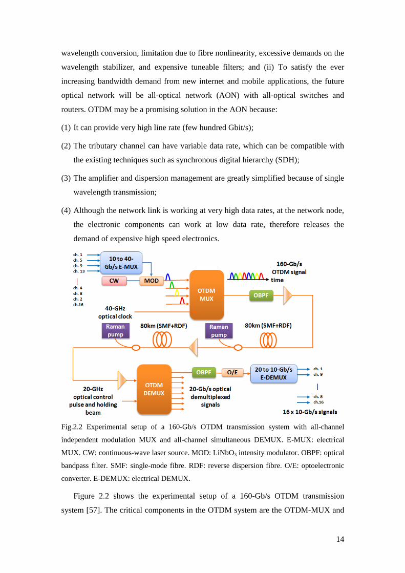
Fig.2.2 Experimental setup of a 160-Gb/s OTDM transmission system with all-channel
independent modulation MUX and all-channel simultaneous DEMUX. E-MUX: electrical
MUX. CW: continuous-wave laser source. MOD: LiNbO3 intensity modulator. OBPF: optical
bandpass filter. SMF: single-mode fibre. RDF: reverse dispersion fibre. O/E: optoelectronic
converter. E-DEMUX: electrical DEMUX.
Figure 2.2 shows the experimental setup of a 160-Gb/s OTDM transmission
system [57]. The critical components in the OTDM system are the OTDM-MUX and
15
OTDM-DEMUX. At the transmitter, an E-MUX multiplexes four 10-Gb/s electrical
signals to a 40-Gb/s signal. The signal is then modulated onto the optical domain with
NRZ modulation format by a LiNbO3 intensity modulator. A 40-GHz optical clock is
also generated by using a mode-locked laser diode and supercontinuum techniques.
By filtering the supercontinuum spectrum, the pulse train is converted to the
appropriate wavelength and pulse width. Four independently generated 40-Gb/s
optical signals and the optical clock are then fed into the OTDM-MUX, which
consists of two 4×1 couplers, a 2×1 coupler and periodically poled lithium niobate
(PPLN) waveguides and integrated on a planar lightwave circuit (PLC). After the
OTDM-MUX, a 160-Gb/s OTDM signal is obtained. The multiplexed signals have
the same polarization in this experiment due to the polarization dependence of PPLN.
However, alternative polarization is possible in other implementations. A 10-GHz
optical clock is also transmitted with 160-Gb/s OTDM signal for clock recovery.
After 160-km SMF+RDF transmission, at the receiver, the OTDM-DEMUX accepts
the 160-Gb/s OTDM signal and 20-GHz optical control pulse (generated from the
recovered 10-GHz clock). The OTDM-DEMUX consists of two 1×8 couplers, 8
WDM couplers and a SOA array. The FWM of SOA yield all-optical de-multiplexing.
A linear polarized pump with polarization controller is also used to de-multiplex the
OTDM signal. The relaxation time of SOAs imposes a limit on the base bit rate of
OTDM-DEMUX, which is 20Gb/s. The eight 20-Gb/s signals are then optically
filtered and converted back to electrical domain through an O/E converter. They are
then electrically de-multiplexed again to 2×10-Gb/s each. Finally, the 16×10-Gb/s
signals are received and processed. It is worth noting that reverse dispersion fibres
(RDFs) are used in the link to compensate the chromatic dispersion (CD) of SMF,
therefore CD is no longer a problem. There are also many challenges in OTDM
systems. For example, at transmitter side, the pulse source must provide a well-
controlled repetition frequency and wavelength [57], e.g., the pulse width should be
significantly shorter than the bit period of the multiplexed data signal and the timing
jitter should be much less than the pulse width. At the receiver side, High quality and
low cost techniques are also needed for the recovery of optical clock and optical de-
multiplexing. For the transmission link, OTDM is very susceptible to dispersions such
as CD and polarization-mode dispersion (PMD), therefore dispersion compensation
must be carefully done (or using optical solitons).
16
2.2.3 Coherent optical OFDM (CO-OFDM)
CO-OFDM represents the ultimate performance in receiver sensitivity, spectral
efficiency and robustness against polarization dispersion, but requires high
complexity in transceiver design. In the open literature, CO-OFDM was first proposed
by Shieh and Athaudage [18], and the concept of the coherent optical MIMO-OFDM
was formalized by Shieh et al. in [58]. The early CO-OFDM experiments were carried
out by Shieh et al. for a 1000 km SSMF transmission at 8 Gb/s [59], and by Jansen et
al. for 4160 km SSMF transmission at 20 Gb/s [ 60 ]. The principle and
transmitter/receiver design for CO-OFDM are given below.
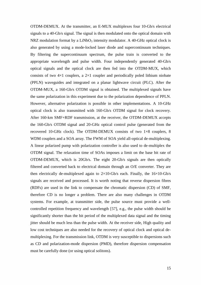
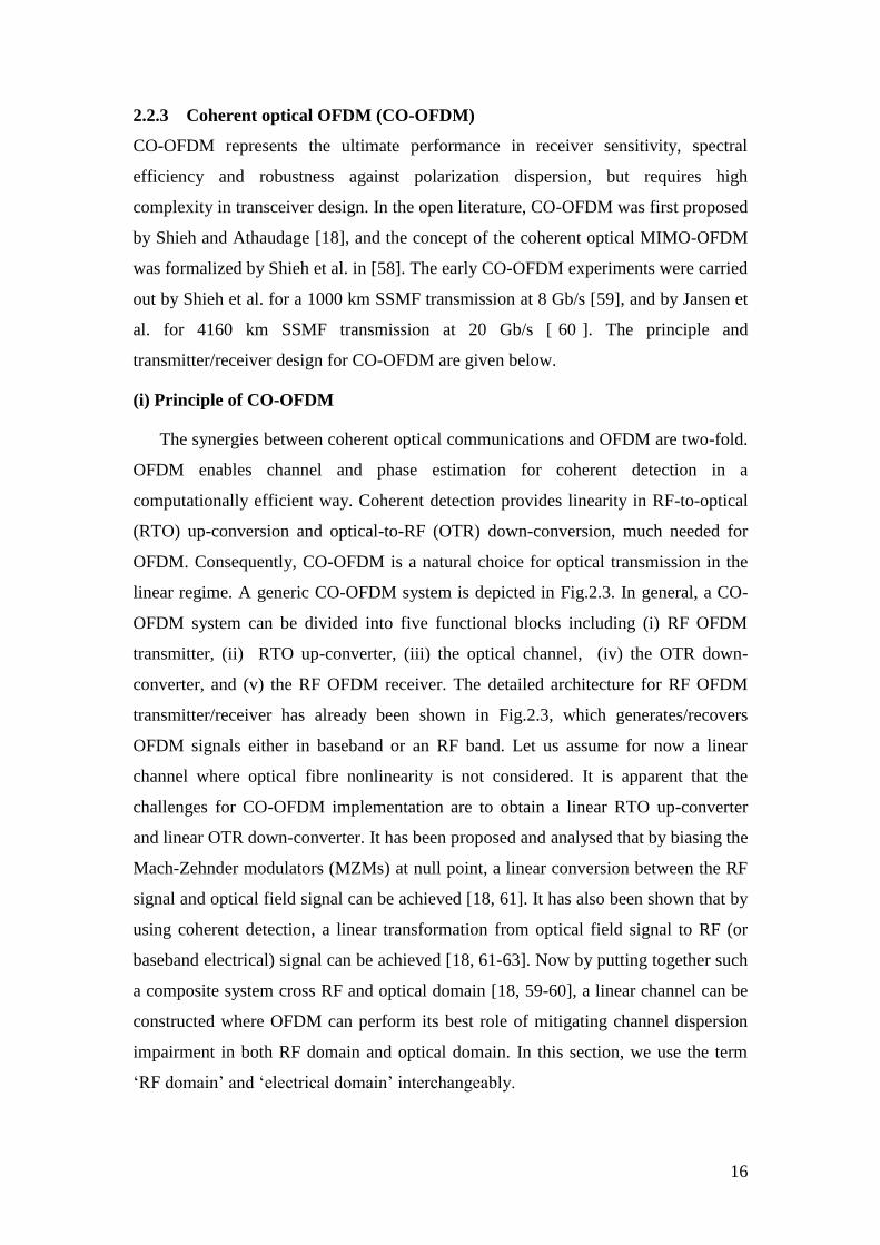
(i) Principle of CO-OFDM
The synergies between coherent optical communications and OFDM are two-fold.
OFDM enables channel and phase estimation for coherent detection in a
computationally efficient way. Coherent detection provides linearity in RF-to-optical
(RTO) up-conversion and optical-to-RF (OTR) down-conversion, much needed for
OFDM. Consequently, CO-OFDM is a natural choice for optical transmission in the
linear regime. A generic CO-OFDM system is depicted in Fig.2.3. In general, a CO-
OFDM system can be divided into five functional blocks including (i) RF OFDM
transmitter, (ii) RTO up-converter, (iii) the optical channel, (iv) the OTR down-
converter, and (v) the RF OFDM receiver. The detailed architecture for RF OFDM
transmitter/receiver has already been shown in Fig.2.3, which generates/recovers
OFDM signals either in baseband or an RF band. Let us assume for now a linear
channel where optical fibre nonlinearity is not considered. It is apparent that the
challenges for CO-OFDM implementation are to obtain a linear RTO up-converter
and linear OTR down-converter. It has been proposed and analysed that by biasing the
Mach-Zehnder modulators (MZMs) at null point, a linear conversion between the RF
signal and optical field signal can be achieved [18, 61]. It has also been shown that by
using coherent detection, a linear transformation from optical field signal to RF (or
baseband electrical) signal can be achieved [18, 61-63]. Now by putting together such
a composite system cross RF and optical domain [18, 59-60], a linear channel can be
constructed where OFDM can perform its best role of mitigating channel dispersion
impairment in both RF domain and optical domain. In this section, we use the term
‘RF domain’ and ‘electrical domain’ interchangeably.
17
Data
-
-
Data
PD1
PD2
PD3
PD4
LD2
RF-to-Optical Up-Converter
I
Q
I
Q
RF-to-Optical Down-Converter
RF OFDM
Transmitter
RF OFDM
Transmitter
RF OFDM
Receiver
RF OFDM
Receiver
MZMMZM
MZMMZM 900900
LD1
900900
(a)
Op
tical L
ink
Data
LD1
LD2
PD2
PD1Data
RF-to-Optical Up-Converter
Optical-to-RF Down-Converter
RF OFDM
Transmitter
RF OFDM
Transmitter
RF OFDM
Receiver
RF OFDM
Receiver
BPFBPF
MZMMZM OBPFⅠOBPFⅠ
OBPFⅡOBPFⅡ
LO1LO1
LO2LO2
BPFBPF
RF IQ Modulator/Demodulator
Op
tical L
ink
-
(b)
Fig.2.3 A CO-OFDM system in (a) direct up/down conversion architecture, and (b)
intermediate frequency (IF) architecture.
: Incoming Signal : Local Oscillator Signal
PD: Photo-detector : Complex photocurrent
-
-
PD1
PD2
PD3
PD4
I
Q
SE
LOE
1
2 s LOE E
1
2 s LOE E
1
2 s LOE jE
1
2 s LOE jE
90 0
Optical
Hybrid
90 0
Optical
Hybrid
I t
SE LOE
*2 s LOI t E E
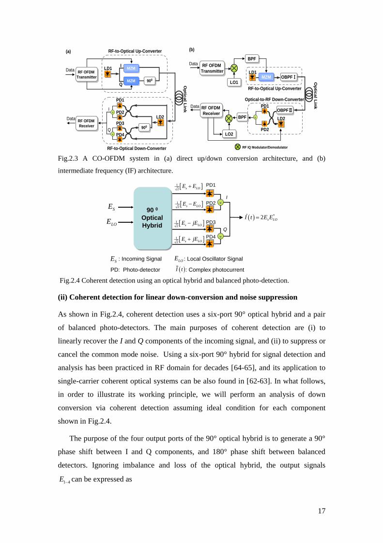
Fig.2.4 Coherent detection using an optical hybrid and balanced photo-detection.
(ii) Coherent detection for linear down-conversion and noise suppression
As shown in Fig.2.4, coherent detection uses a six-port 90° optical hybrid and a pair
of balanced photo-detectors. The main purposes of coherent detection are (i) to
linearly recover the I and Q components of the incoming signal, and (ii) to suppress or
cancel the common mode noise. Using a six-port 90° hybrid for signal detection and
analysis has been practiced in RF domain for decades [64-65], and its application to
single-carrier coherent optical systems can be also found in [62-63]. In what follows,
in order to illustrate its working principle, we will perform an analysis of down
conversion via coherent detection assuming ideal condition for each component
shown in Fig.2.4.
The purpose of the four output ports of the 90° optical hybrid is to generate a 90°
phase shift between I and Q components, and 180° phase shift between balanced
detectors. Ignoring imbalance and loss of the optical hybrid, the output signals
1 4E can be expressed as
18
1 11 22 2
1 13 42 2
,
,
s LO s LO
s LO s LO
E E E E E E
E E jE E E jE
(2.1)
where sE and LOE are respectively the incoming signal and local oscillator (LO) signal.
We further decompose the incoming signal into two components: (i) the received
signal when there is no amplified spontaneous noise (ASE), rE t and (ii) the ASE
noise, on t , namely
s r oE E n (2.2)
We first study how the I component of the photo-detected current is generated, and
the Q component can be derived accordingly. The I component is obtained by using a
pair of the photo-detectors, PD1 and PD2 in Fig.2.4, whose photocurrent 1 2I can be
described as
2 2 2 *
1 1
12Re
2s LO s LOI E E E E E (2.3)
2 2 2 *
2 2
12Re
2s LO s LOI E E E E E (2.4)
2 2 2 *2Res r o r oE E n E n (2.5)
2
1LO LO RINE I I t (2.6)
where LOI and RINI t are the average power and relative intensity noise (RIN) of the
LO laser, and ‘Re’ or ‘Im’ denotes the real or imaginary part of a complex signal. For
simplicity, the photo-detection responsivity is set to unity. The three terms at the right
hand of (2.5) represent signal-to-signal beat noise, signal-to-ASE beat noise, and
ASE-to-ASE beat noise. Because of the balanced detection, using (2.3) and (2.4), the I
component of the photocurrent becomes
*
1 2 2ReI s LOI t I I E E (2.7)
Now the noise suppression mechanism becomes quite clear because the three noise
terms in (2.5) and the RIN noise in (2.6) from a single detector are completely
cancelled via balanced detection. Nevertheless, it has been shown that coherent
detection can be performed by using a single photo-detector, but at the cost of reduced
dynamic range [66].
19
In a similar fashion, the Q component from the other pair of balanced detectors
can be derived as
*
3 4 2ImQ s LOI t I I E E (2.8)
Using the results of (2.7) and (2.8), the complex detected signal I (t)consisting of both
I and Q components becomes
*2I Q s LOI t I t jI t E E (2.9)
From (2.9), the linear down-conversion process via coherent detection becomes quite
clear; the complex photocurrent I (t) is in essence a linear replica of the incoming
complex signal that is frequency down-converted by a local oscillator frequency. Thus
with linear coherent detection at receiver and linear generation at transmitter, complex
OFDM signals can be readily transmitted over the optical fibre channel.
2.2.4 Direct detection optical OFDM (DDO-OFDM)
A DDO-OFDM aim for simpler transmitter/receiver than CO-OFDM for lower costs.
It has many variants which reflect the different requirements in terms of data rates and
costs from a broad range of applications. For instance, the first report of the DDO-
OFDM [67] takes advantage of the fact the OFDM signal is more immune to the
impulse clipping noise seen in CATV networks. Another example is single-side-band
(SSB)-OFDM which has been recently proposed by Lowery et al. and Djordjevic et al.
for long-haul transmission [22, 68 ]. Tang et al. have proposed an adaptively
modulated optical OFDM (AMO-OFDM) that uses bit and power loading showing
promising results for both multimode fibre and short-reach SMF fibre links [20, 69-
70]. The common feature for DDO-OFDM is use of a simple square-law photodiode
at the receiver. DDO-OFDM can be divided into two categories according to how
optical OFDM signal is being generated: (i) linearly-mapped DDO-OFDM (LM-
DDO-OFDM) where the optical OFDM spectrum is a replica of baseband OFDM, and
(ii) nonlinearly-mapped DDO-OFDM (NLM-DDO-OFDM) where the optical OFDM
spectrum does not display a replica of baseband OFDM. In what follows, we discuss
the principles and design choices for these two classes of direct-detection OFDM
systems.
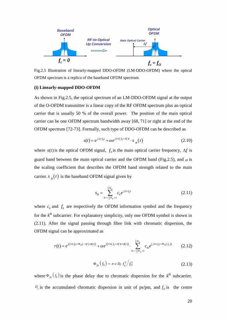
20
Main Optical Carrier
Baseband
OFDM
fc = 0fc = fO
RF-to-Optical
Up Conversion
Optical
OFDM
f
Fig.2.5 Illustration of linearly-mapped DDO-OFDM (LM-DDO-OFDM) where the optical
OFDM spectrum is a replica of the baseband OFDM spectrum.
(i) Linearly-mapped DDO-OFDM
As shown in Fig.2.5, the optical spectrum of an LM-DDO-OFDM signal at the output
of the O-OFDM transmitter is a linear copy of the RF OFDM spectrum plus an optical
carrier that is usually 50 % of the overall power. The position of the main optical
carrier can be one OFDM spectrum bandwidth away [68, 71] or right at the end of the
OFDM spectrum [72-73]. Formally, such type of DDO-OFDM can be described as
00
22( )
j f f tj f t
Bs t e e s t
(2.10)
where ( )s t is the optical OFDM signal, 0f is the main optical carrier frequency, f is
guard band between the main optical carrier and the OFDM band (Fig.2.5), and is
the scaling coefficient that describes the OFDM band strength related to the main
carrier. B
s t is the baseband OFDM signal given by
12
12
2
1
sc
k
sc
N
j f t
B k
k N
s c e
(2.11)
where kc and kf are respectively the OFDM information symbol and the frequency
for the kth
subcarrier. For explanatory simplicity, only one OFDM symbol is shown in
(2.11). After the signal passing through fibre link with chromatic dispersion, the
OFDM signal can be approximated as
12
00
12
2 22
1
( )sc
k D kD
sc
Nj f f t t j f t fj f t f t
ik
k N
r t e e c e
(2.12)
2 2k t OD k
f c D f f (2.13)
where kDf is the phase delay due to chromatic dispersion for the k
th subcarrier.
tD is the accumulated chromatic dispersion in unit of ps/pm, and Of is the centre
21
frequency of optical OFDM spectrum, and c is the speed of light. At the receiver, the
photodetector can be modelled as a square-law detector and the resultant photo-
current signal is
12
12
1 12 2
1 2 1 2
2 11 1
1 22 2
2 22
1
22 *
1 1
1 2 Resc
k D k D
sc
sc sc
k k D k D k
sc sc
Nj f t f fj ft
ik
k N
N Nj f f t f f
k k
k N k N
I t r t e c e
c c e
(2.14)
The first term is a DC component that can be easily filtered out. The second term is
the fundamental term consisting linear OFDM subcarriers that are to be retrieved. The
third term is the second-order nonlinearity term that needs to be removed.
There are several approaches to minimize the penalty due to the second-order
nonlinearity term:
(A) Offset SSB-OFDM. Sufficient guard band is allocated such that the second-term
and third-term RF spectra are non-overlapping. As such, the third term in Eq.
(2.14) can be easily removed using a RF or DSP filter, as proposed by Lowery et
al. in [68].
(B) Baseband Optical SSB-OFDM. coefficient is reduced as much as possible such
that the distortion as result of the third-term is reduced to an acceptable level.
This approach has been adopted by Djordjevic et al. [22] and Hewitt et al. [72].
(C) Subcarrier interleaving. From Eq. (2.14), it follows that if only odd subcarriers
are filled, i.e., kc is nonzero only for the odd subcarriers, the second-order
intermodulation will be at even subcarriers, which are orthogonal to the original
signal at the odd subcarrier frequencies. Subsequently, the third-term does not
produce any interference. This approach has been proposed by Peng et al. [74].
(D) Iterative distortion reduction. The basic idea is to go through a number of
iterations of estimation of the linear term, and compute the second-order term
using the estimated linear term, and removing the second-order term from the
right side of Eq. (2.14). This approach has been proposed by Peng et al. [73].
There are advantages and disadvantages among all these four approaches. For
instance, Approach B has the advantage of better spectral efficiency, but at the cost of
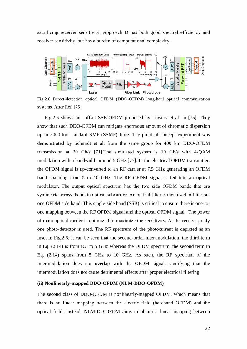
22
sacrificing receiver sensitivity. Approach D has both good spectral efficiency and
receiver sensitivity, but has a burden of computational complexity.
a.u. Modulator Drive Power [dBm] OSA Power [dBm] RX
Laser Fiber Link Photodiode
Frequency [GHz]Time [ns]
Fig.2.6 Direct-detection optical OFDM (DDO-OFDM) long-haul optical communication
systems. After Ref. [75]
Fig.2.6 shows one offset SSB-OFDM proposed by Lowery et al. in [75]. They
show that such DDO-OFDM can mitigate enormous amount of chromatic dispersion
up to 5000 km standard SMF (SSMF) fibre. The proof-of-concept experiment was
demonstrated by Schmidt et al. from the same group for 400 km DDO-OFDM
transmission at 20 Gb/s [71].The simulated system is 10 Gb/s with 4-QAM
modulation with a bandwidth around 5 GHz [75]. In the electrical OFDM transmitter,
the OFDM signal is up-converted to an RF carrier at 7.5 GHz generating an OFDM
band spanning from 5 to 10 GHz. The RF OFDM signal is fed into an optical
modulator. The output optical spectrum has the two side OFDM bands that are
symmetric across the main optical subcarrier. An optical filter is then used to filter out
one OFDM side band. This single-side band (SSB) is critical to ensure there is one-to-
one mapping between the RF OFDM signal and the optical OFDM signal. The power
of main optical carrier is optimized to maximize the sensitivity. At the receiver, only
one photo-detector is used. The RF spectrum of the photocurrent is depicted as an
inset in Fig.2.6. It can be seen that the second-order inter-modulation, the third-term
in Eq. (2.14) is from DC to 5 GHz whereas the OFDM spectrum, the second term in
Eq. (2.14) spans from 5 GHz to 10 GHz. As such, the RF spectrum of the
intermodulation does not overlap with the OFDM signal, signifying that the
intermodulation does not cause detrimental effects after proper electrical filtering.
(ii) Nonlinearly-mapped DDO-OFDM (NLM-DDO-OFDM)
The second class of DDO-OFDM is nonlinearly-mapped OFDM, which means that
there is no linear mapping between the electric field (baseband OFDM) and the
optical field. Instead, NLM-DD-OFDM aims to obtain a linear mapping between
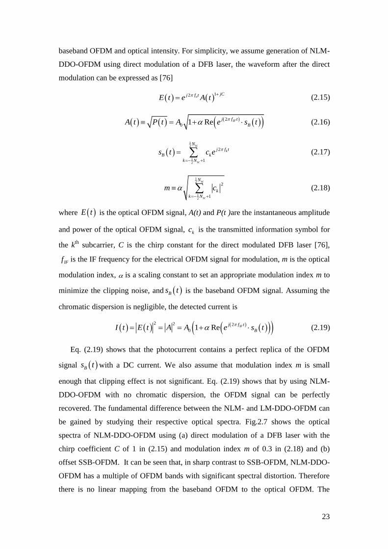
23
baseband OFDM and optical intensity. For simplicity, we assume generation of NLM-
DDO-OFDM using direct modulation of a DFB laser, the waveform after the direct
modulation can be expressed as [76]
12 o
jCj f tE t e A t
(2.15)
2
0 1 Re IFj f t
BA t P t A e s t
(2.16)
12
12
2
1
sc
k
sc
N
j f t
B k
k N
s t c e
(2.17)
12
12
2
1
sc
sc
N
k
k N
m c
(2.18)
where E t is the optical OFDM signal, A(t) and P(t )are the instantaneous amplitude
and power of the optical OFDM signal, kc is the transmitted information symbol for
the kth
subcarrier, C is the chirp constant for the direct modulated DFB laser [76],
IFf is the IF frequency for the electrical OFDM signal for modulation, m is the optical
modulation index, is a scaling constant to set an appropriate modulation index m to
minimize the clipping noise, and Bs t is the baseband OFDM signal. Assuming the
chromatic dispersion is negligible, the detected current is
2 2 2
0 1 Re IFj f t
BI t E t A A e s t
(2.19)
Eq. (2.19) shows that the photocurrent contains a perfect replica of the OFDM
signal Bs t with a DC current. We also assume that modulation index m is small
enough that clipping effect is not significant. Eq. (2.19) shows that by using NLM-
DDO-OFDM with no chromatic dispersion, the OFDM signal can be perfectly
recovered. The fundamental difference between the NLM- and LM-DDO-OFDM can
be gained by studying their respective optical spectra. Fig.2.7 shows the optical
spectra of NLM-DDO-OFDM using (a) direct modulation of a DFB laser with the
chirp coefficient C of 1 in (2.15) and modulation index m of 0.3 in (2.18) and (b)
offset SSB-OFDM. It can be seen that, in sharp contrast to SSB-OFDM, NLM-DDO-
OFDM has a multiple of OFDM bands with significant spectral distortion. Therefore
there is no linear mapping from the baseband OFDM to the optical OFDM. The
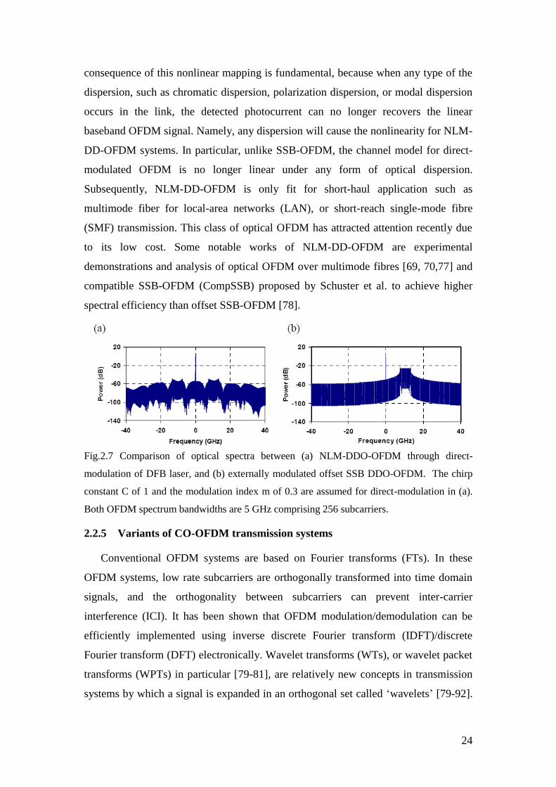
24
consequence of this nonlinear mapping is fundamental, because when any type of the
dispersion, such as chromatic dispersion, polarization dispersion, or modal dispersion
occurs in the link, the detected photocurrent can no longer recovers the linear
baseband OFDM signal. Namely, any dispersion will cause the nonlinearity for NLM-
DD-OFDM systems. In particular, unlike SSB-OFDM, the channel model for direct-
modulated OFDM is no longer linear under any form of optical dispersion.
Subsequently, NLM-DD-OFDM is only fit for short-haul application such as
multimode fiber for local-area networks (LAN), or short-reach single-mode fibre
(SMF) transmission. This class of optical OFDM has attracted attention recently due
to its low cost. Some notable works of NLM-DD-OFDM are experimental
demonstrations and analysis of optical OFDM over multimode fibres [69, 70,77] and
compatible SSB-OFDM (CompSSB) proposed by Schuster et al. to achieve higher
spectral efficiency than offset SSB-OFDM [78].
Fig.2.7 Comparison of optical spectra between (a) NLM-DDO-OFDM through direct-
modulation of DFB laser, and (b) externally modulated offset SSB DDO-OFDM. The chirp
constant C of 1 and the modulation index m of 0.3 are assumed for direct-modulation in (a).
Both OFDM spectrum bandwidths are 5 GHz comprising 256 subcarriers.
2.2.5 Variants of CO-OFDM transmission systems
Conventional OFDM systems are based on Fourier transforms (FTs). In these
OFDM systems, low rate subcarriers are orthogonally transformed into time domain
signals, and the orthogonality between subcarriers can prevent inter-carrier
interference (ICI). It has been shown that OFDM modulation/demodulation can be
efficiently implemented using inverse discrete Fourier transform (IDFT)/discrete
Fourier transform (DFT) electronically. Wavelet transforms (WTs), or wavelet packet
transforms (WPTs) in particular [79-81], are relatively new concepts in transmission
systems by which a signal is expanded in an orthogonal set called ‘wavelets’ [79-92].
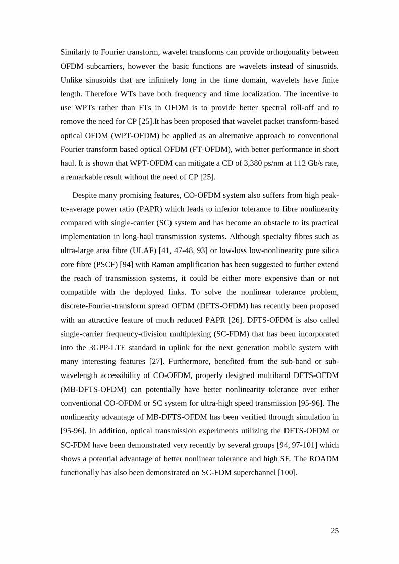
25
Similarly to Fourier transform, wavelet transforms can provide orthogonality between
OFDM subcarriers, however the basic functions are wavelets instead of sinusoids.
Unlike sinusoids that are infinitely long in the time domain, wavelets have finite
length. Therefore WTs have both frequency and time localization. The incentive to
use WPTs rather than FTs in OFDM is to provide better spectral roll-off and to
remove the need for CP [25].It has been proposed that wavelet packet transform-based
optical OFDM (WPT-OFDM) be applied as an alternative approach to conventional
Fourier transform based optical OFDM (FT-OFDM), with better performance in short
haul. It is shown that WPT-OFDM can mitigate a CD of 3,380 ps/nm at 112 Gb/s rate,
a remarkable result without the need of CP [25].
Despite many promising features, CO-OFDM system also suffers from high peak-
to-average power ratio (PAPR) which leads to inferior tolerance to fibre nonlinearity
compared with single-carrier (SC) system and has become an obstacle to its practical
implementation in long-haul transmission systems. Although specialty fibres such as
ultra-large area fibre (ULAF) [41, 47-48, 93] or low-loss low-nonlinearity pure silica
core fibre (PSCF) [94] with Raman amplification has been suggested to further extend
the reach of transmission systems, it could be either more expensive than or not
compatible with the deployed links. To solve the nonlinear tolerance problem,
discrete-Fourier-transform spread OFDM (DFTS-OFDM) has recently been proposed
with an attractive feature of much reduced PAPR [26]. DFTS-OFDM is also called
single-carrier frequency-division multiplexing (SC-FDM) that has been incorporated
into the 3GPP-LTE standard in uplink for the next generation mobile system with
many interesting features [27]. Furthermore, benefited from the sub-band or sub-
wavelength accessibility of CO-OFDM, properly designed multiband DFTS-OFDM
(MB-DFTS-OFDM) can potentially have better nonlinearity tolerance over either
conventional CO-OFDM or SC system for ultra-high speed transmission [95-96]. The
nonlinearity advantage of MB-DFTS-OFDM has been verified through simulation in
[95-96]. In addition, optical transmission experiments utilizing the DFTS-OFDM or
SC-FDM have been demonstrated very recently by several groups [94, 97-101] which
shows a potential advantage of better nonlinear tolerance and high SE. The ROADM
functionally has also been demonstrated on SC-FDM superchannel [100].
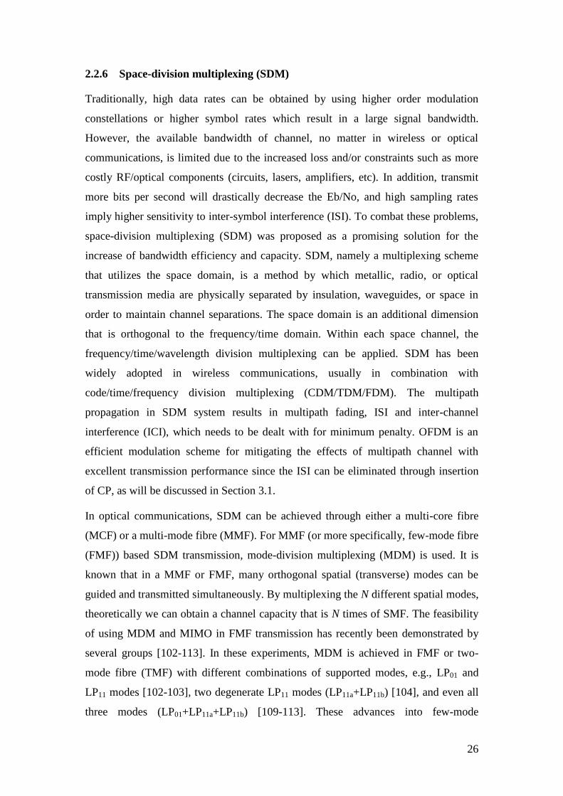
26
2.2.6 Space-division multiplexing (SDM)
Traditionally, high data rates can be obtained by using higher order modulation
constellations or higher symbol rates which result in a large signal bandwidth.
However, the available bandwidth of channel, no matter in wireless or optical
communications, is limited due to the increased loss and/or constraints such as more
costly RF/optical components (circuits, lasers, amplifiers, etc). In addition, transmit
more bits per second will drastically decrease the Eb/No, and high sampling rates
imply higher sensitivity to inter-symbol interference (ISI). To combat these problems,
space-division multiplexing (SDM) was proposed as a promising solution for the
increase of bandwidth efficiency and capacity. SDM, namely a multiplexing scheme
that utilizes the space domain, is a method by which metallic, radio, or optical
transmission media are physically separated by insulation, waveguides, or space in
order to maintain channel separations. The space domain is an additional dimension
that is orthogonal to the frequency/time domain. Within each space channel, the
frequency/time/wavelength division multiplexing can be applied. SDM has been
widely adopted in wireless communications, usually in combination with
code/time/frequency division multiplexing (CDM/TDM/FDM). The multipath
propagation in SDM system results in multipath fading, ISI and inter-channel
interference (ICI), which needs to be dealt with for minimum penalty. OFDM is an
efficient modulation scheme for mitigating the effects of multipath channel with
excellent transmission performance since the ISI can be eliminated through insertion
of CP, as will be discussed in Section 3.1.
In optical communications, SDM can be achieved through either a multi-core fibre
(MCF) or a multi-mode fibre (MMF). For MMF (or more specifically, few-mode fibre
(FMF)) based SDM transmission, mode-division multiplexing (MDM) is used. It is
known that in a MMF or FMF, many orthogonal spatial (transverse) modes can be
guided and transmitted simultaneously. By multiplexing the N different spatial modes,
theoretically we can obtain a channel capacity that is N times of SMF. The feasibility
of using MDM and MIMO in FMF transmission has recently been demonstrated by
several groups [102-113]. In these experiments, MDM is achieved in FMF or two-
mode fibre (TMF) with different combinations of supported modes, e.g., LP01 and
LP11 modes [102-103], two degenerate LP11 modes (LP11a+LP11b) [104], and even all
three modes (LP01+LP11a+LP11b) [109-113]. These advances into few-mode
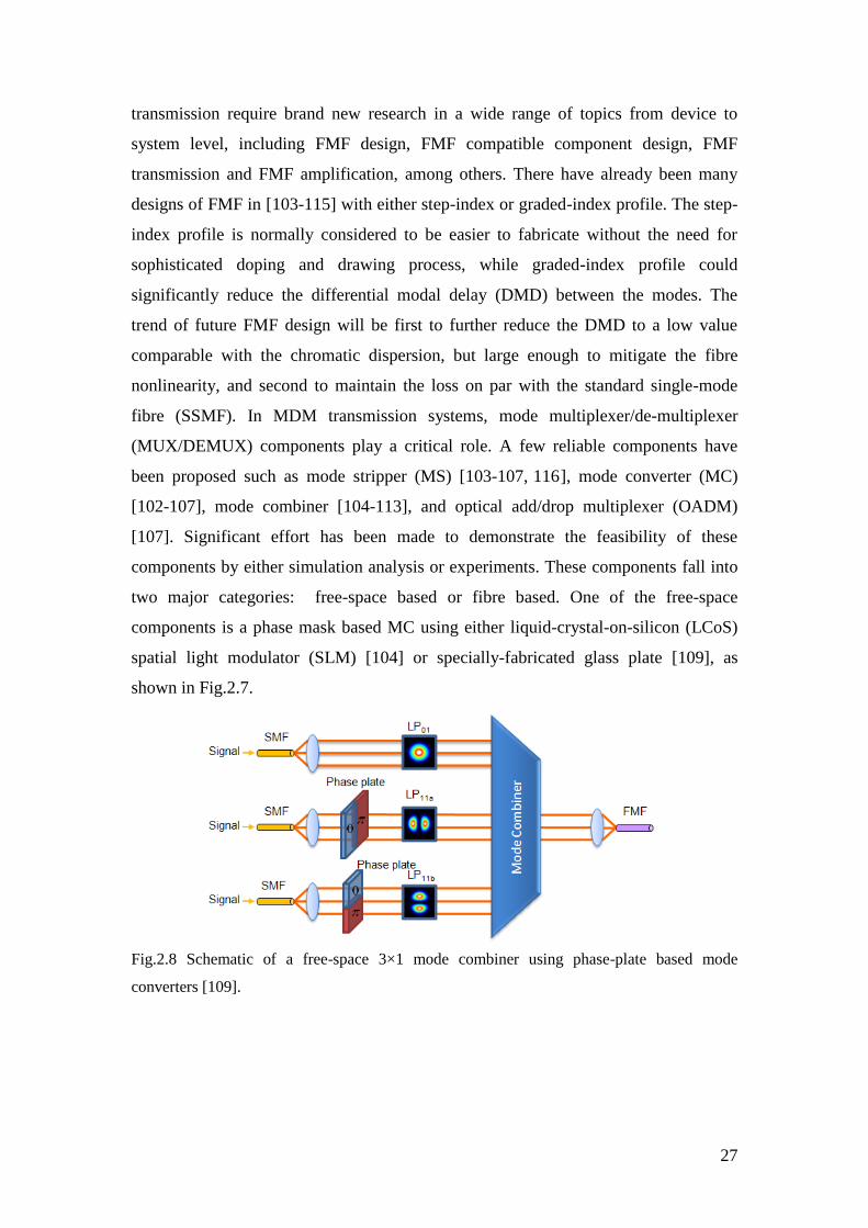
27
transmission require brand new research in a wide range of topics from device to
system level, including FMF design, FMF compatible component design, FMF
transmission and FMF amplification, among others. There have already been many
designs of FMF in [103-115] with either step-index or graded-index profile. The step-
index profile is normally considered to be easier to fabricate without the need for
sophisticated doping and drawing process, while graded-index profile could
significantly reduce the differential modal delay (DMD) between the modes. The
trend of future FMF design will be first to further reduce the DMD to a low value
comparable with the chromatic dispersion, but large enough to mitigate the fibre
nonlinearity, and second to maintain the loss on par with the standard single-mode
fibre (SSMF). In MDM transmission systems, mode multiplexer/de-multiplexer
(MUX/DEMUX) components play a critical role. A few reliable components have
been proposed such as mode stripper (MS) [103-107, 116], mode converter (MC)
[102-107], mode combiner [104-113], and optical add/drop multiplexer (OADM)
[107]. Significant effort has been made to demonstrate the feasibility of these
components by either simulation analysis or experiments. These components fall into
two major categories: free-space based or fibre based. One of the free-space
components is a phase mask based MC using either liquid-crystal-on-silicon (LCoS)
spatial light modulator (SLM) [104] or specially-fabricated glass plate [109], as
shown in Fig.2.7.
Fig.2.8 Schematic of a free-space 3×1 mode combiner using phase-plate based mode
converters [109].
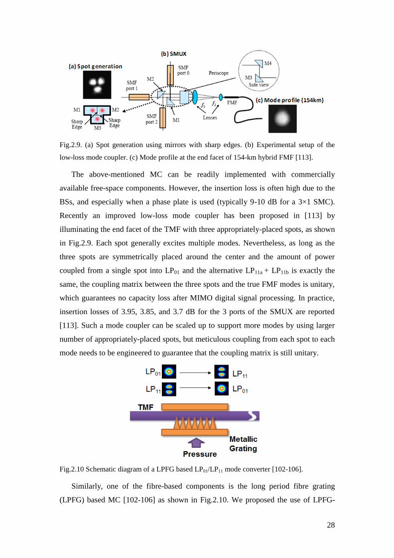
28
Fig.2.9. (a) Spot generation using mirrors with sharp edges. (b) Experimental setup of the
low-loss mode coupler. (c) Mode profile at the end facet of 154-km hybrid FMF [113].
The above-mentioned MC can be readily implemented with commercially
available free-space components. However, the insertion loss is often high due to the
BSs, and especially when a phase plate is used (typically 9-10 dB for a 3×1 SMC).
Recently an improved low-loss mode coupler has been proposed in [113] by
illuminating the end facet of the TMF with three appropriately-placed spots, as shown
in Fig.2.9. Each spot generally excites multiple modes. Nevertheless, as long as the
three spots are symmetrically placed around the center and the amount of power
coupled from a single spot into LP01 and the alternative LP11a + LP11b is exactly the
same, the coupling matrix between the three spots and the true FMF modes is unitary,
which guarantees no capacity loss after MIMO digital signal processing. In practice,
insertion losses of 3.95, 3.85, and 3.7 dB for the 3 ports of the SMUX are reported
[113]. Such a mode coupler can be scaled up to support more modes by using larger
number of appropriately-placed spots, but meticulous coupling from each spot to each
mode needs to be engineered to guarantee that the coupling matrix is still unitary.
Fig.2.10 Schematic diagram of a LPFG based LP01/LP11 mode converter [102-106].
Similarly, one of the fibre-based components is the long period fibre grating
(LPFG) based MC [102-106] as shown in Fig.2.10. We proposed the use of LPFG-

29
based MC as a practical solution for MMUX/MDEMUX in MDM transmission. Its
mechanism, fabrication and characterization will be discussed in Section 6.2.
Experimental demonstration of MDM transmission utilizing the LPFG-based MC will
be further shown in Chapter 7. The advantage of fibre based components over their
free-space counterparts is the compactness and easiness of integration.
Beside the mode MUMX/MDEMUX components, few-mode amplifier for FMF
transmission is also very important if there is significant accumulation of loss. The
loss could come from the mode MUX/DEMUX or fibre loss. The feasibility of few-
mode amplification using EDFA or Raman pump has recently been demonstrated
[117-120] with the inclusion of aforementioned MCs. FMF compatible EDFA opens a
gate to the long-haul FMF transmission [112, 117-119]. As is well known, the
nonlinear effects in silica fibre impose a hard constraint on the achievable channel
capacity. For FMF based transmission, there is strong field overlapping between
different modes thus it is important to analyse the FMF systems taking into account
potential inter-modal nonlinearity [121]. There have already been many theoretical
studies on the nonlinear propagation modelling and simulation of FMF based
transmission systems [121-122], but the experimental result is lacking. In a recent
work [123] we have shown for the first time the experimental characterization of
nonlinear parameters in a FMF. We have also proposed a method to mitigate the
nonlinear noise on subsystem level, namely the unique-word DFT-Spread OFDM
(UW-DFTS-OFDM) [95-99] which could fit well for future Terabit/s SDM
superchannel transmission.
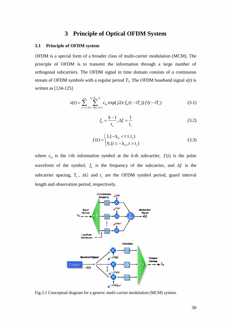
30
3 Principle of Optical OFDM System
3.1 Principle of OFDM system
OFDM is a special form of a broader class of multi-carrier modulation (MCM). The
principle of OFDM is to transmit the information through a large number of
orthogonal subcarriers. The OFDM signal in time domain consists of a continuous
stream of OFDM symbols with a regular period Ts. The OFDM baseband signal s(t) is
written as [124-125]
/2
/2 1
( ) exp( 2 ( )) ( )sck N
ki k s s
i k Nsc
s t c j f t iT f t iT
(3.1)
1 1
,k
s s
kf f
t t
(3.2)
1,( )
( )0, ( , )
G s
G s
t tf t
t t t
(3.3)
where kic is the i-th information symbol at the k-th subcarrier, ( )f t is the pulse
waveform of the symbol, kf is the frequency of the subcarrier, and f is the
subcarrier spacing, sT , G and st are the OFDM symbol period, guard interval
length and observation period, respectively.
Fig.3.1 Conceptual diagram for a generic multi-carrier modulation (MCM) system.
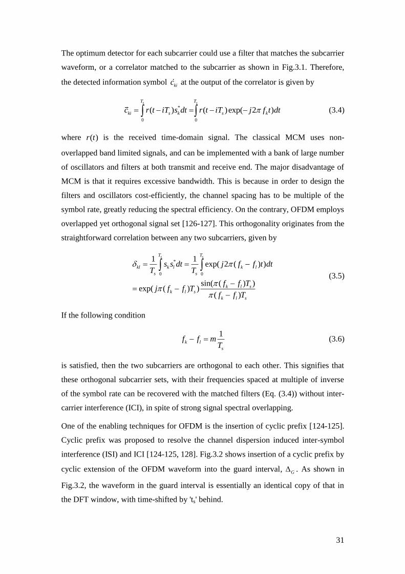
31
The optimum detector for each subcarrier could use a filter that matches the subcarrier
waveform, or a correlator matched to the subcarrier as shown in Fig.3.1. Therefore,
the detected information symbol kic at the output of the correlator is given by
*
0 0
( ) ( )exp( 2 )s sT T
ki s k s kc r t iT s dt r t iT j f t dt (3.4)
where ( )r t is the received time-domain signal. The classical MCM uses non-
overlapped band limited signals, and can be implemented with a bank of large number
of oscillators and filters at both transmit and receive end. The major disadvantage of
MCM is that it requires excessive bandwidth. This is because in order to design the
filters and oscillators cost-efficiently, the channel spacing has to be multiple of the
symbol rate, greatly reducing the spectral efficiency. On the contrary, OFDM employs
overlapped yet orthogonal signal set [126-127]. This orthogonality originates from the
straightforward correlation between any two subcarriers, given by
*
0 0
1 1exp( 2 ( ) )
sin( ( ) )exp( ( ) )
( )
s sT T
kl k l k l
s s
k l sk l s
k l s
s s dt j f f t dtT T
f f Tj f f T
f f T
(3.5)
If the following condition
1
k l
s
f f mT
(3.6)
is satisfied, then the two subcarriers are orthogonal to each other. This signifies that
these orthogonal subcarrier sets, with their frequencies spaced at multiple of inverse
of the symbol rate can be recovered with the matched filters (Eq. (3.4)) without inter-
carrier interference (ICI), in spite of strong signal spectral overlapping.
One of the enabling techniques for OFDM is the insertion of cyclic prefix [124-125].
Cyclic prefix was proposed to resolve the channel dispersion induced inter-symbol
interference (ISI) and ICI [124-125, 128]. Fig.3.2 shows insertion of a cyclic prefix by
cyclic extension of the OFDM waveform into the guard interval, G . As shown in
Fig.3.2, the waveform in the guard interval is essentially an identical copy of that in
the DFT window, with time-shifted by 'ts' behind.
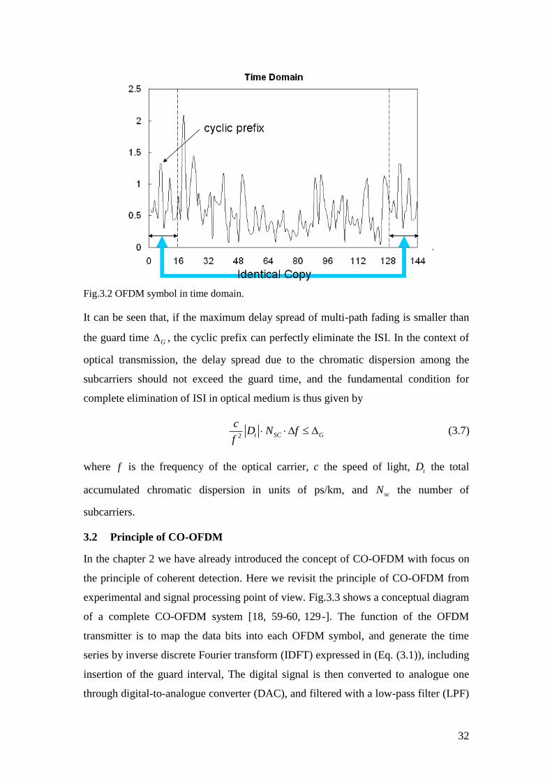
32
Fig.3.2 OFDM symbol in time domain.
It can be seen that, if the maximum delay spread of multi-path fading is smaller than
the guard time G , the cyclic prefix can perfectly eliminate the ISI. In the context of
optical transmission, the delay spread due to the chromatic dispersion among the
subcarriers should not exceed the guard time, and the fundamental condition for
complete elimination of ISI in optical medium is thus given by
2 t SC G
cD N f
f (3.7)
where f is the frequency of the optical carrier, c the speed of light, tD the total
accumulated chromatic dispersion in units of ps/km, and scN the number of
subcarriers.
3.2 Principle of CO-OFDM
In the chapter 2 we have already introduced the concept of CO-OFDM with focus on
the principle of coherent detection. Here we revisit the principle of CO-OFDM from
experimental and signal processing point of view. Fig.3.3 shows a conceptual diagram
of a complete CO-OFDM system [18, 59-60, 129-]. The function of the OFDM
transmitter is to map the data bits into each OFDM symbol, and generate the time
series by inverse discrete Fourier transform (IDFT) expressed in (Eq. (3.1)), including
insertion of the guard interval, The digital signal is then converted to analogue one
through digital-to-analogue converter (DAC), and filtered with a low-pass filter (LPF)
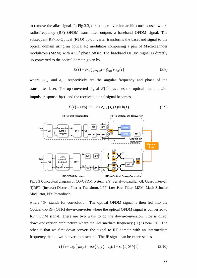
33
to remove the alias signal. In Fig.3.3, direct-up conversion architecture is used where
radio-frequency (RF) OFDM transmitter outputs a baseband OFDM signal. The
subsequent RF-To-Optical (RTO) up-converter transforms the baseband signal to the
optical domain using an optical IQ modulator comprising a pair of Mach-Zehnder
modulators (MZM) with a 90o phase offset. The baseband OFDM signal is directly
up-converted to the optical domain given by
1 1exp LD LD BE t j t s t (3.8)
where 1LD and
1LD respectively are the angular frequency and phase of the
transmitter laser. The up-converted signal E t traverses the optical medium with
impulse response ( )h t , and the received optical signal becomes
1 1exp LD LD BE t j t s t h t (3.9)
Data Subcarrier
symbol
mapper
Subcarrier
symbol
mapperS/PS/P IDFTIDFT GIGI
D/AD/A LPFLPF
……
……
D/AD/A LPFLPF
I
Q
MZMMZM
MZMMZM 900900LD1
I
LPFLPF
LPFLPF
A/DA/D
A/DA/D
DFTDFT
Data
symbol
Decision
&
Equalization
Data
symbol
Decision
&
Equalization
P/SP/S
……
……
-
-
PD1
PD2
PD3
PD4
LD2
RF-to-Optical Down-Converter
900900
Q
Data
RF-to-Optical Up-Converter
Optical
Link
Optical
Link
Re
Im
Optical I/Q
Modulator
RF OFDM Transmitter
RF OFDM Receiver Fig.3.3 Conceptual diagram of CO-OFDM system. S/P: Serial-to-parallel, GI: Guard Interval,
(I)DFT: (Inverse) Discrete Fourier Transform, LPF: Low Pass Filter, MZM: Mach-Zehnder
Modulator, PD: Photodiode.
where ' ' stands for convolution. The optical OFDM signal is then fed into the
Optical-To-RF (OTR) down-converter where the optical OFDM signal is converted to
RF OFDM signal. There are two ways to do the down-conversion. One is direct
down-conversion architecture where the intermediate frequency (IF) is near DC. The
other is that we first down-convert the signal to RF domain with an intermediate
frequency then down-convert to baseband. The IF signal can be expressed as
0 0exp , ( )off Br t j t r t r t s t h t (3.10)
34
1 2 1 2,off LD LD LD LD (3.11)
where off and are respectively the angular frequency offset and phase offset
between transmit and receive lasers. In the RF OFDM receiver, the down-converted
OFDM signal is first sampled with an analogue-to-digital converter (ADC). Then the
signal needs to go through sophisticated three levels of synchronizations before the
symbol decision can be made. The three levels of synchronizations are (i) FFT
window synchronization where OFDM symbol is properly delineated to avoid inter-
symbol-interference, (ii) frequency synchronization, namely, frequency offset off
needs to be estimated and compensated, and (iii) the subcarrier recovery, where each
subcarrier channel is estimated and compensated. Assuming successful completion of
DFT window synchronization and frequency synchronization, the RF OFDM signal
through DFT of the sampled value of Eq. (3.10) becomes
i
ki ki ki kir e h c n
(3.12)
where kir is the received information symbol, i is the OFDM symbol phase (OSP) or
common phase error (CPE), kih is the frequency domain channel transfer function, kin
is the noise. The third synchronization of subcarrier recovery involves estimation of
OSP i and the channel transfer function kih . Once they are known, an estimated
value of kic , kic is given by zero-forcing method as
*
2
ki i
ki
i
ki
ki
hc e r
h
(3.13)
kic is used for symbol decision or to recover the transmitter value kic , which is
subsequently be mapped back to the original transmitted digital bits.
The above description of CO-OFDM processing has so far leaved out the pilot-
subcarrier or training-symbol insertion where a proportion of the subcarriers or all the
subcarriers in one OFDM symbol are known values to the receiver. The purpose of
these pilot subcarrier or training symbol is to assist the above-mentioned three-level
synchronization. Another important aspect of the CO-OFDM signal processing that is
not discussed is the error-correction coding involving error-correction
encoder/decoder, and interleaver/de-interleaver.
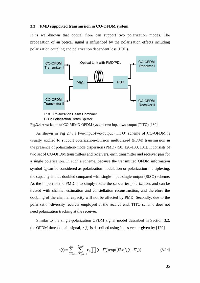
35
3.3 PMD supported transmission in CO-OFDM system
It is well-known that optical fibre can support two polarization modes. The
propagation of an optical signal is influenced by the polarization effects including
polarization coupling and polarization dependent loss (PDL).
Fig.3.4 A variation of CO-MIMO-OFDM system: two-input two-output (TITO) [130].
As shown in Fig 2.4, a two-input-two-output (TITO) scheme of CO-OFDM is
usually applied to support polarization-division multiplexed (PDM) transmission in
the presence of polarization-mode dispersion (PMD) [58, 128-130, 131]. It consists of
two set of CO-OFDM transmitters and receivers, each transmitter and receiver pair for
a single polarization. In such a scheme, because the transmitted OFDM information
symbol kic can be considered as polarization modulation or polarization multiplexing,
the capacity is thus doubled compared with single-input-single-output (SISO) scheme.
As the impact of the PMD is to simply rotate the subcarrier polarization, and can be
treated with channel estimation and constellation reconstruction, and therefore the
doubling of the channel capacity will not be affected by PMD. Secondly, due to the
polarization-diversity receiver employed at the receive end, TITO scheme does not
need polarization tracking at the receiver.
Similar to the single-polarization OFDM signal model described in Section 3.2,
the OFDM time-domain signal, )(ts is described using Jones vector given by [129]
/2
/2 1
( ) ( )exp 2 ( )sc
sc
N
ik s k s
i k N
t t iT j f t iT
s c (3.14)
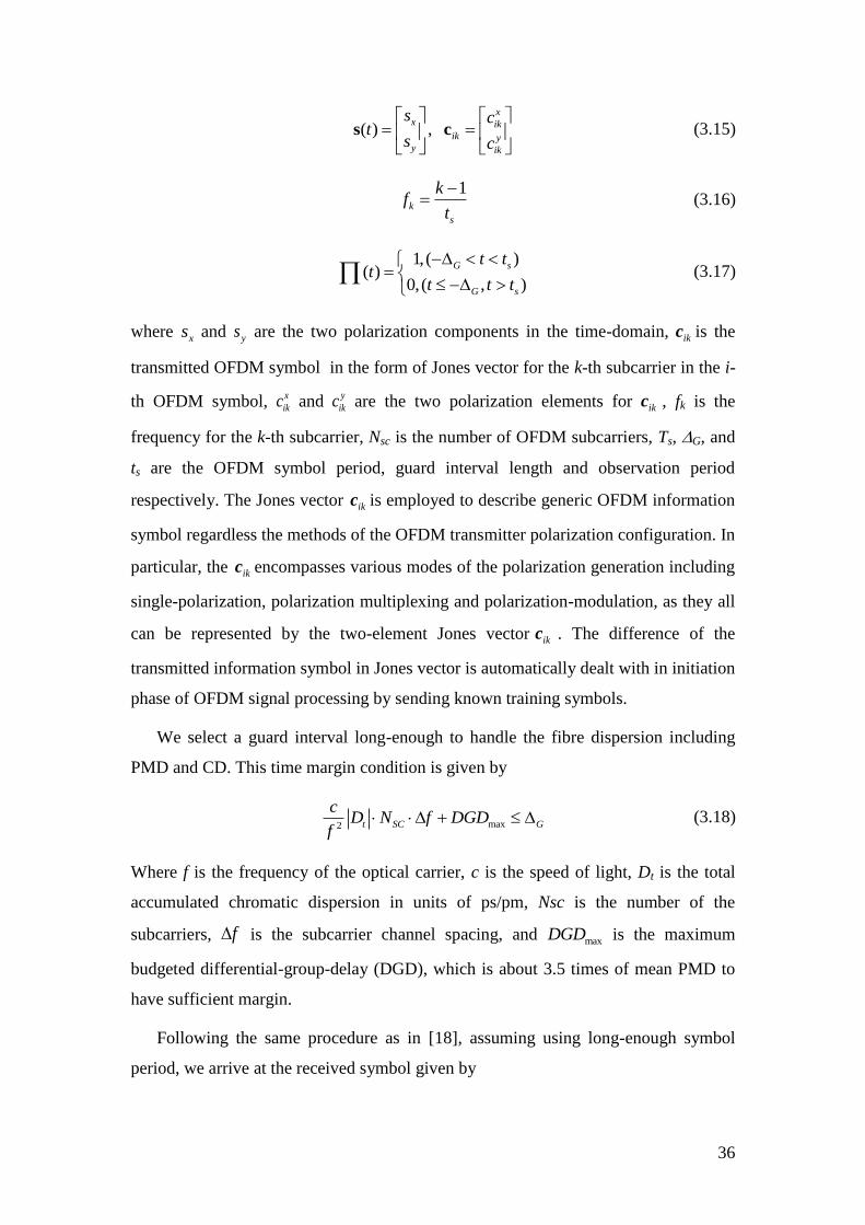
36
( ) ,x
x ik
ik yy ik
s ct
s c
s c (3.15)
1
k
s
kf
t
(3.16)
1,( )
( )0, ( , )
G s
G s
t tt
t t t
(3.17)
where xs and ys are the two polarization components in the time-domain, ikc is the
transmitted OFDM symbol in the form of Jones vector for the k-th subcarrier in the i-
th OFDM symbol, x
ikc and y
ikc are the two polarization elements for ikc , fk is the
frequency for the k-th subcarrier, Nsc is the number of OFDM subcarriers, Ts, G, and
ts are the OFDM symbol period, guard interval length and observation period
respectively. The Jones vector ikc is employed to describe generic OFDM information
symbol regardless the methods of the OFDM transmitter polarization configuration. In
particular, the ikc encompasses various modes of the polarization generation including
single-polarization, polarization multiplexing and polarization-modulation, as they all
can be represented by the two-element Jones vector ikc . The difference of the
transmitted information symbol in Jones vector is automatically dealt with in initiation
phase of OFDM signal processing by sending known training symbols.
We select a guard interval long-enough to handle the fibre dispersion including
PMD and CD. This time margin condition is given by
max2 t SC G
cD N f DGD
f (3.18)
Where f is the frequency of the optical carrier, c is the speed of light, Dt is the total
accumulated chromatic dispersion in units of ps/pm, Nsc is the number of the
subcarriers, f is the subcarrier channel spacing, and maxDGD is the maximum
budgeted differential-group-delay (DGD), which is about 3.5 times of mean PMD to
have sufficient margin.
Following the same procedure as in [18], assuming using long-enough symbol
period, we arrive at the received symbol given by
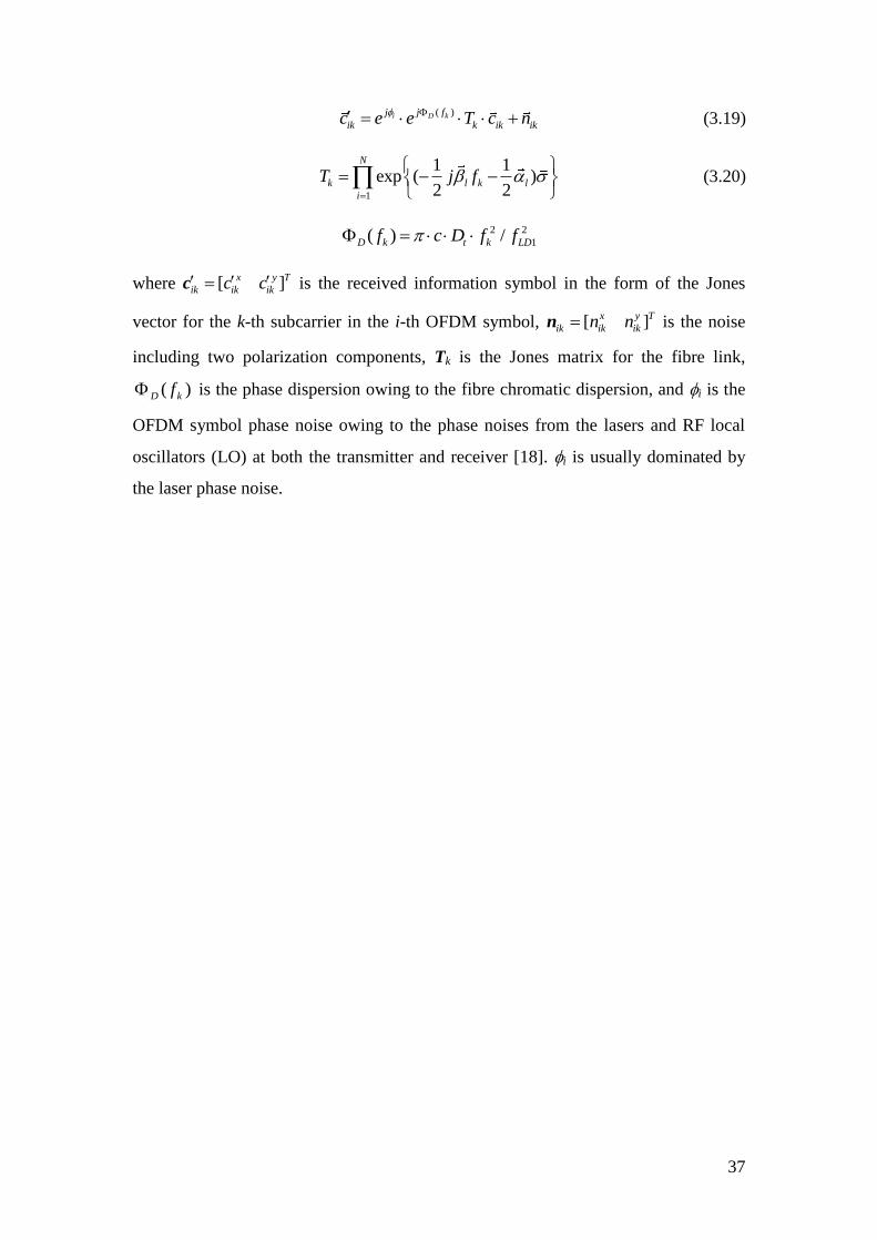
37
( )i D kj j f
ik k ik ikc e e T c n (3.19)
1
1 1exp ( )
2 2
N
k l k l
i
T j f
(3.20)
2 2
1( ) /D k t k LDf c D f f
where Ty
ik
x
ikik cc ][ c is the received information symbol in the form of the Jones
vector for the k-th subcarrier in the i-th OFDM symbol, Ty
ik
x
ikik nn ][n is the noise
including two polarization components, Tk is the Jones matrix for the fibre link,
)( kD f is the phase dispersion owing to the fibre chromatic dispersion, and i is the
OFDM symbol phase noise owing to the phase noises from the lasers and RF local
oscillators (LO) at both the transmitter and receiver [18]. i is usually dominated by
the laser phase noise.
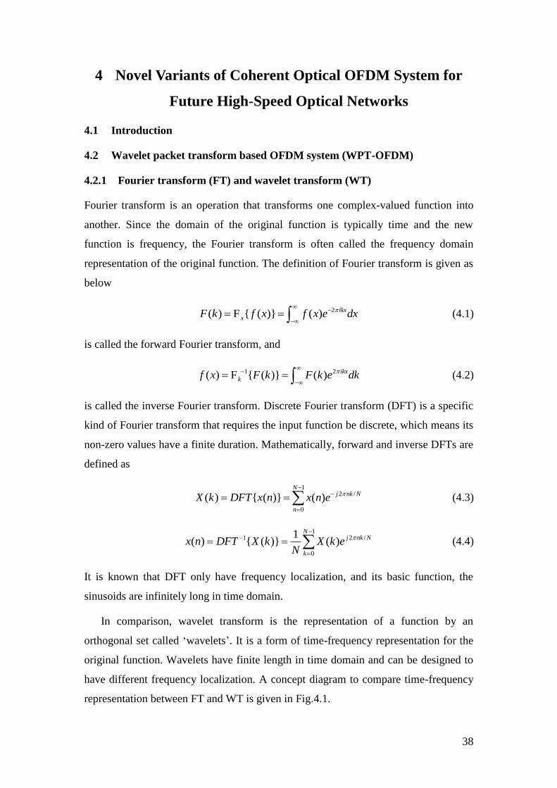
38
4 Novel Variants of Coherent Optical OFDM System for
Future High-Speed Optical Networks
4.1 Introduction
4.2 Wavelet packet transform based OFDM system (WPT-OFDM)
4.2.1 Fourier transform (FT) and wavelet transform (WT)
Fourier transform is an operation that transforms one complex-valued function into
another. Since the domain of the original function is typically time and the new
function is frequency, the Fourier transform is often called the frequency domain
representation of the original function. The definition of Fourier transform is given as
below
2( ) { ( )} ( ) ikx
xF k f x f x e dx
F (4.1)
is called the forward Fourier transform, and
1 2( ) { ( )} ( ) ikx
kf x F k F k e dk
F (4.2)
is called the inverse Fourier transform. Discrete Fourier transform (DFT) is a specific
kind of Fourier transform that requires the input function be discrete, which means its
non-zero values have a finite duration. Mathematically, forward and inverse DFTs are
defined as
1
2 /
0
( ) { ( )} ( )N
j nk N
n
X k DFT x n x n e
(4.3)
1
1 2 /
0
1( ) { ( )} ( )
Nj nk N
k
x n DFT X k X k eN
(4.4)
It is known that DFT only have frequency localization, and its basic function, the
sinusoids are infinitely long in time domain.
In comparison, wavelet transform is the representation of a function by an
orthogonal set called ‘wavelets’. It is a form of time-frequency representation for the
original function. Wavelets have finite length in time domain and can be designed to
have different frequency localization. A concept diagram to compare time-frequency
representation between FT and WT is given in Fig.4.1.
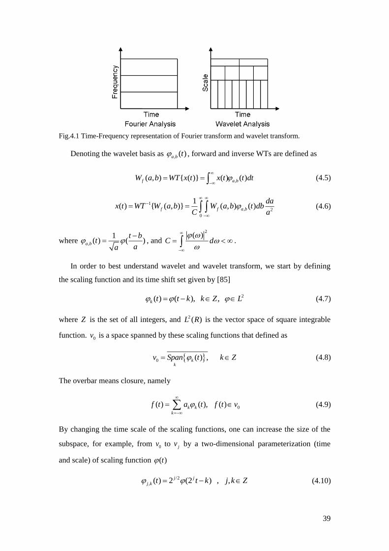
39
Fig.4.1 Time-Frequency representation of Fourier transform and wavelet transform.
Denoting the wavelet basis as , ( )a b t , forward and inverse WTs are defined as
,( , ) { ( )} ( ) ( )f a bW a b WT x t x t t dt
(4.5)
1
, 2
0
1( ) { ( , )} ( , ) ( )f f a b
dax t WT W a b W a b t db
C a
(4.6)
where ,
1( ) ( )a b
t bt
aa
, and
2( )
C d
.
In order to best understand wavelet and wavelet transform, we start by defining
the scaling function and its time shift set given by [85]
2( ) ( ), ,k t t k k Z L (4.7)
where Z is the set of all integers, and 2 ( )L R is the vector space of square integrable
function. 0v is a space spanned by these scaling functions that defined as
0 ( ) ,kk
v Span t k Z (4.8)
The overbar means closure, namely
0( ) ( ), ( )k k
k
f t a t f t v
(4.9)
By changing the time scale of the scaling functions, one can increase the size of the
subspace, for example, from 0v to jv by a two-dimensional parameterization (time
and scale) of scaling function ( )t
/2
, ( ) 2 (2 ) , ,j j
j k t t k j k Z (4.10)
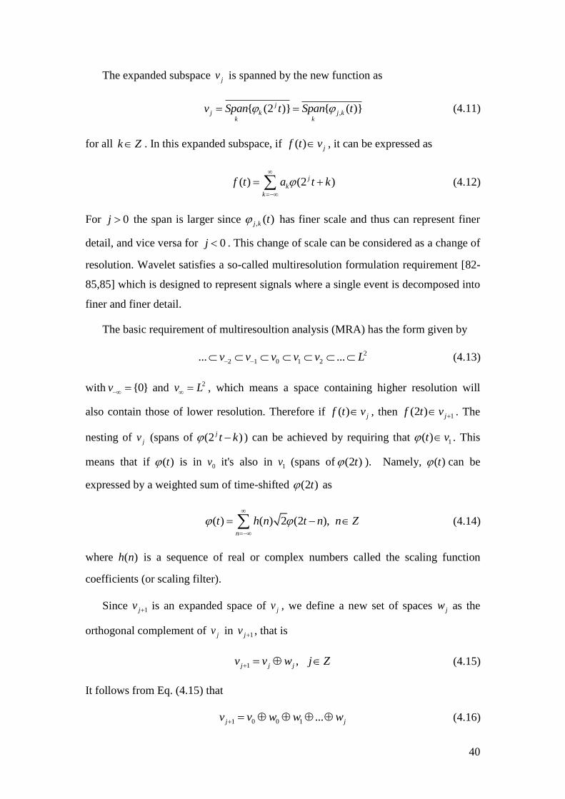
40
The expanded subspace jv is spanned by the new function as
,{ (2 )} { ( )}j
j k j kk k
v Span t Span t (4.11)
for all k Z . In this expanded subspace, if ( ) jf t v , it can be expressed as
( ) (2 )j
k
k
f t a t k
(4.12)
For 0j the span is larger since , ( )j k t has finer scale and thus can represent finer
detail, and vice versa for 0j . This change of scale can be considered as a change of
resolution. Wavelet satisfies a so-called multiresolution formulation requirement [82-
85,85] which is designed to represent signals where a single event is decomposed into
finer and finer detail.
The basic requirement of multiresoultion analysis (MRA) has the form given by
2
2 1 0 1 2... ...v v v v v L (4.13)
with {0}v and 2v L , which means a space containing higher resolution will
also contain those of lower resolution. Therefore if ( ) jf t v , then 1(2 ) jf t v . The
nesting of jv (spans of (2 )j t k ) can be achieved by requiring that 1( )t v . This
means that if ( )t is in 0v it's also in 1v (spans of (2 )t ). Namely, ( )t can be
expressed by a weighted sum of time-shifted (2 )t as
( ) ( ) 2 (2 ),n
t h n t n n Z
(4.14)
where ( )h n is a sequence of real or complex numbers called the scaling function
coefficients (or scaling filter).
Since 1jv is an expanded space of jv , we define a new set of spaces jw as the
orthogonal complement of jv in 1jv , that is
1 ,j j jv v w j Z (4.15)
It follows from Eq. (4.15) that
1 0 0 1 ...j jv v w w w (4.16)
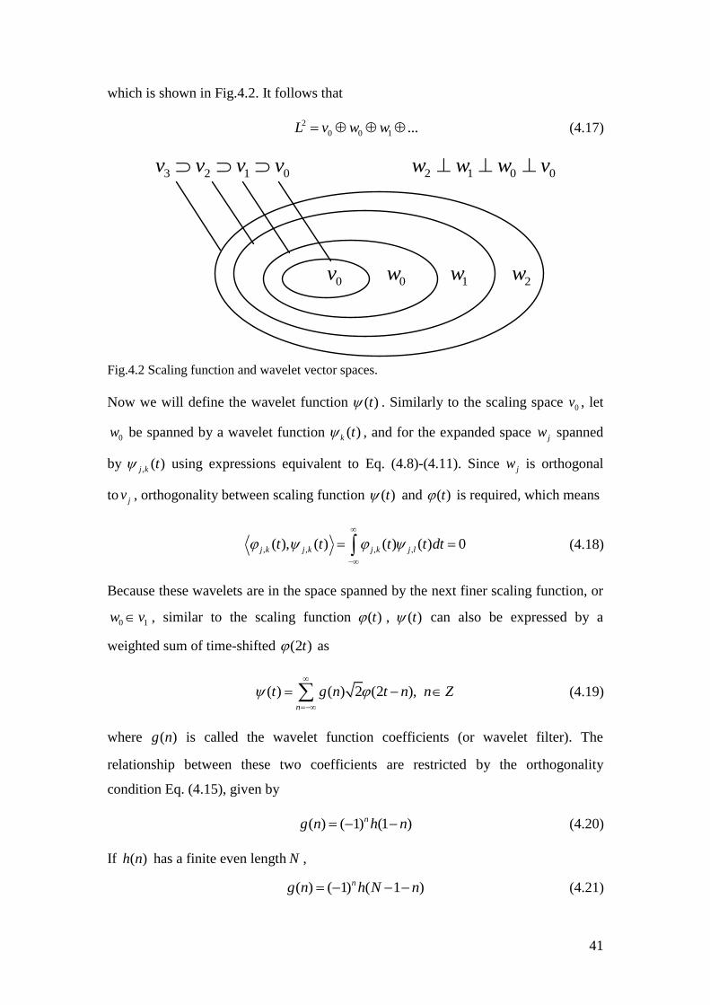
41
which is shown in Fig.4.2. It follows that
2
0 0 1 ...L v w w (4.17)
3 2 1 0v v v v 2 1 0 0w w w v
0 0 1 2v w w w
Fig.4.2 Scaling function and wavelet vector spaces.
Now we will define the wavelet function ( )t . Similarly to the scaling space 0v , let
0w be spanned by a wavelet function ( )k t , and for the expanded space jw spanned
by , ( )j k t using expressions equivalent to Eq. (4.8)-(4.11). Since jw is orthogonal
to jv , orthogonality between scaling function ( )t and ( )t is required, which means
, , , ,( ), ( ) ( ) ( ) 0j k j k j k j lt t t t dt
(4.18)
Because these wavelets are in the space spanned by the next finer scaling function, or
0 1w v , similar to the scaling function ( )t , ( )t can also be expressed by a
weighted sum of time-shifted (2 )t as
( ) ( ) 2 (2 ),n
t g n t n n Z
(4.19)
where ( )g n is called the wavelet function coefficients (or wavelet filter). The
relationship between these two coefficients are restricted by the orthogonality
condition Eq. (4.15), given by
( ) ( 1) (1 )ng n h n (4.20)
If ( )h n has a finite even length N ,
( ) ( 1) ( 1 )ng n h N n (4.21)
42
In addition, for the wavelet coefficients ( )g n , an orthonormal perfect reconstruction
(PR) requirement usually applies. PR means that in the absence of encoding,
quantization and transmission errors, the reconstructed signal can be perfectly
reassembled at the receiver, which is critical for transmission system. The
orthonormality condition and the perfect reconstruction condition of the orthonormal
two bands PR filter are [82]
1Tg g (4.22)
and
( ) ( 2 ) ( )n
g n g n k k
(4.23)
where g in Eq. (4.22) is the vector form of ( )g n .
We now use Haar wavelet to explain the wavelet and scaling coefficients. Haar
wavelet function ( )t is
1 0 1/ 2,
( ) 1 1/ 2 1,
0 .
t
t t
otherwise
(4.24)
and its scaling function is
1 0 1,
( )0 .
tt
otherwise
(4.25)
The filter coefficients of Haar wavelet can be obtained by applying Eqs. (4.14) and
(4.19) given by
1 1
( ) ( 1, 1) , ( ) (1, 1)2 2
h n g n (4.26)
Now we have defined scaling and wavelet function as well as scaling and wavelet
coefficients. From the wavelet theory we know that for any arbitrary signal we can
expand it into a sum of scaling and wavelet functions, and this process is called
wavelet transform (WT). Similarly to the Fourier transform, wavelet transform also
has a discrete analogue called discrete wavelet transform (DWT). The discrete
wavelet expansion of any signal 2( ) ( )f t L R is given by
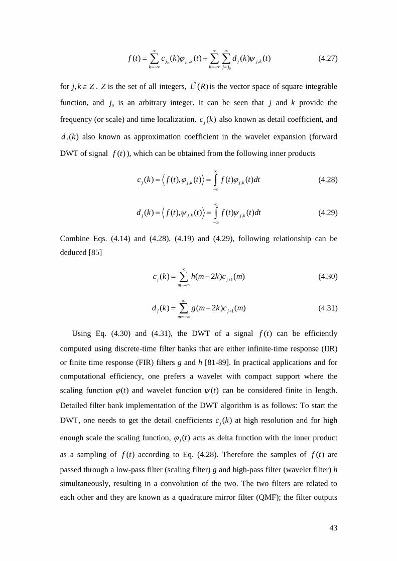
43
0 0
0
, ,( ) ( ) ( ) ( ) ( )j j k j j k
k k j j
f t c k t d k t
(4.27)
for ,j k Z . Z is the set of all integers, 2 ( )L R is the vector space of square integrable
function, and 0j is an arbitrary integer. It can be seen that j and k provide the
frequency (or scale) and time localization. ( )jc k also known as detail coefficient, and
( )jd k also known as approximation coefficient in the wavelet expansion (forward
DWT of signal ( )f t ), which can be obtained from the following inner products
, ,( ) ( ), ( ) ( ) ( )j j k j kc k f t t f t t dt
(4.28)
, ,( ) ( ), ( ) ( ) ( )j j k j kd k f t t f t t dt
(4.29)
Combine Eqs. (4.14) and (4.28), (4.19) and (4.29), following relationship can be
deduced [85]
1( ) ( 2 ) ( )j j
m
c k h m k c m
(4.30)
1( ) ( 2 ) ( )j j
m
d k g m k c m
(4.31)
Using Eq. (4.30) and (4.31), the DWT of a signal ( )f t can be efficiently
computed using discrete-time filter banks that are either infinite-time response (IIR)
or finite time response (FIR) filters g and h [81-89]. In practical applications and for
computational efficiency, one prefers a wavelet with compact support where the
scaling function ( )t and wavelet function ( )t can be considered finite in length.
Detailed filter bank implementation of the DWT algorithm is as follows: To start the
DWT, one needs to get the detail coefficients ( )jc k at high resolution and for high
enough scale the scaling function, ( ) j t acts as delta function with the inner product
as a sampling of ( )f t according to Eq. (4.28). Therefore the samples of ( )f t are
passed through a low-pass filter (scaling filter) g and high-pass filter (wavelet filter) h
simultaneously, resulting in a convolution of the two. The two filters are related to
each other and they are known as a quadrature mirror filter (QMF); the filter outputs
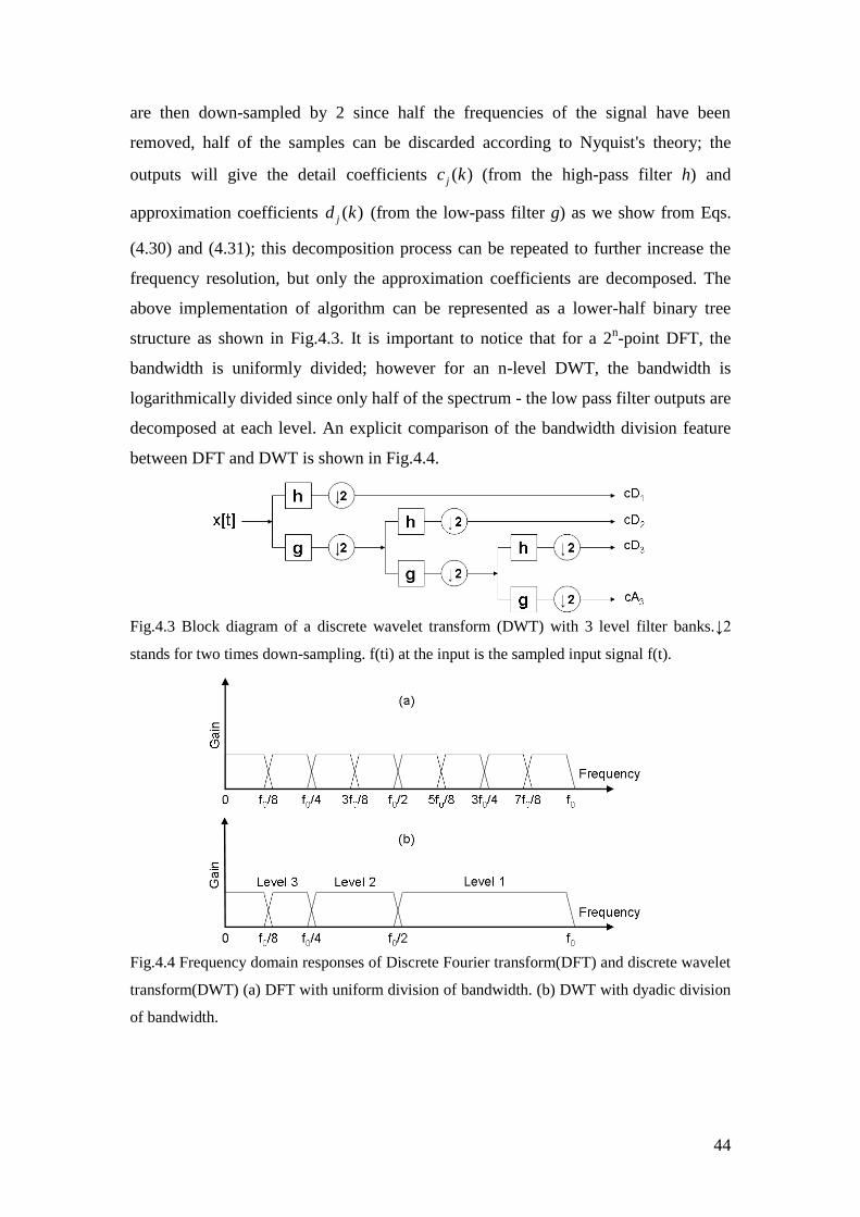
44
are then down-sampled by 2 since half the frequencies of the signal have been
removed, half of the samples can be discarded according to Nyquist's theory; the
outputs will give the detail coefficients ( )jc k (from the high-pass filter h) and
approximation coefficients ( )jd k (from the low-pass filter g) as we show from Eqs.
(4.30) and (4.31); this decomposition process can be repeated to further increase the
frequency resolution, but only the approximation coefficients are decomposed. The
above implementation of algorithm can be represented as a lower-half binary tree
structure as shown in Fig.4.3. It is important to notice that for a 2n-point DFT, the
bandwidth is uniformly divided; however for an n-level DWT, the bandwidth is
logarithmically divided since only half of the spectrum - the low pass filter outputs are
decomposed at each level. An explicit comparison of the bandwidth division feature
between DFT and DWT is shown in Fig.4.4.
Fig.4.3 Block diagram of a discrete wavelet transform (DWT) with 3 level filter banks.↓2
stands for two times down-sampling. f(ti) at the input is the sampled input signal f(t).
Fig.4.4 Frequency domain responses of Discrete Fourier transform(DFT) and discrete wavelet
transform(DWT) (a) DFT with uniform division of bandwidth. (b) DWT with dyadic division
of bandwidth.
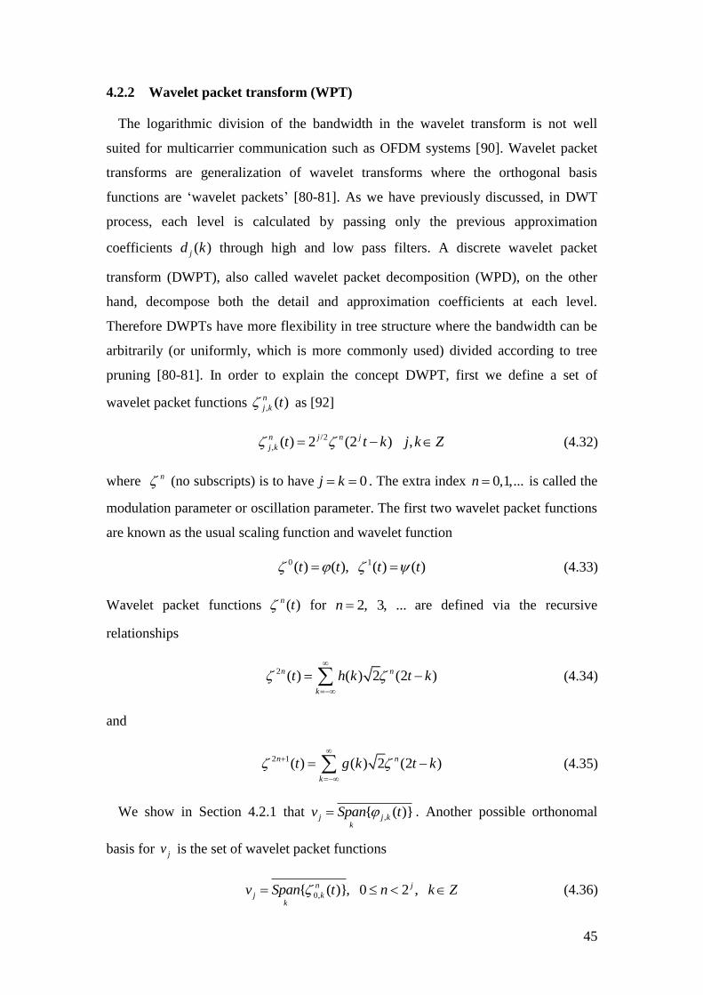
45
4.2.2 Wavelet packet transform (WPT)
The logarithmic division of the bandwidth in the wavelet transform is not well
suited for multicarrier communication such as OFDM systems [90]. Wavelet packet
transforms are generalization of wavelet transforms where the orthogonal basis
functions are ‘wavelet packets’ [80-81]. As we have previously discussed, in DWT
process, each level is calculated by passing only the previous approximation
coefficients ( )jd k through high and low pass filters. A discrete wavelet packet
transform (DWPT), also called wavelet packet decomposition (WPD), on the other
hand, decompose both the detail and approximation coefficients at each level.
Therefore DWPTs have more flexibility in tree structure where the bandwidth can be
arbitrarily (or uniformly, which is more commonly used) divided according to tree
pruning [80-81]. In order to explain the concept DWPT, first we define a set of
wavelet packet functions , ( )n
j k t as [92]
/2
, ( ) 2 (2 ) ,n j n j
j k t t k j k Z (4.32)
where n (no subscripts) is to have 0j k . The extra index 0,1,...n is called the
modulation parameter or oscillation parameter. The first two wavelet packet functions
are known as the usual scaling function and wavelet function
0 1( ) ( ), ( ) ( )t t t t (4.33)
Wavelet packet functions ( ) n t for 2, 3, ...n are defined via the recursive
relationships
2 ( ) ( ) 2 (2 )n n
k
t h k t k
(4.34)
and
2 1( ) ( ) 2 (2 )n n
k
t g k t k
(4.35)
We show in Section 4.2.1 that ,{ ( )}j j kk
v Span t . Another possible orthonomal
basis for jv is the set of wavelet packet functions
0,{ ( )}, 0 2 ,n j
j kk
v Span t n k Z (4.36)
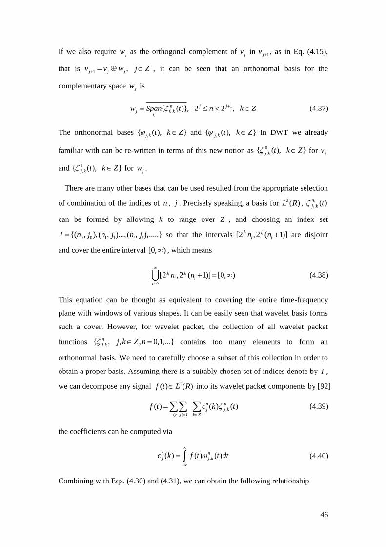
46
If we also require jw as the orthogonal complement of jv in 1jv , as in Eq. (4.15),
that is 1 ,j j jv v w j Z , it can be seen that an orthonomal basis for the
complementary space jw is
1
0,{ ( )}, 2 2 ,n j j
j kk
w Span t n k Z (4.37)
The orthonormal bases ,{ ( ), }j k t k Z and ,{ ( ), }j k t k Z in DWT we already
familiar with can be re-written in terms of this new notion as 0
,{ ( ), } j k t k Z for jv
and 1
,{ ( ), } j k t k Z for jw .
There are many other bases that can be used resulted from the appropriate selection
of combination of the indices of n , j . Precisely speaking, a basis for 2 ( )L R , , ( ) i
i
n
j k t
can be formed by allowing k to range over Z , and choosing an index set
0 0 1 1{( , ),( , )..., ( , ),.....} i iI n j n j n j so that the intervals [2 ,2 ( 1)]i ij j
i in n are disjoint
and cover the entire interval [0, ) , which means
0
[2 ,2 ( 1)] [0, )i ij j
i i
i
n n
(4.38)
This equation can be thought as equivalent to covering the entire time-frequency
plane with windows of various shapes. It can be easily seen that wavelet basis forms
such a cover. However, for wavelet packet, the collection of all wavelet packet
functions ,{ , , , 0,1,...} n
j k j k Z n contains too many elements to form an
orthonormal basis. We need to carefully choose a subset of this collection in order to
obtain a proper basis. Assuming there is a suitably chosen set of indices denote by I ,
we can decompose any signal 2( ) ( )f t L R into its wavelet packet components by [92]
,
( , )
( ) ( ) ( )n n
j j k
n j I k Z
f t c k t
(4.39)
the coefficients can be computed via
,( ) ( ) ( )n n
j j kc k f t t dt
(4.40)
Combining with Eqs. (4.30) and (4.31), we can obtain the following relationship
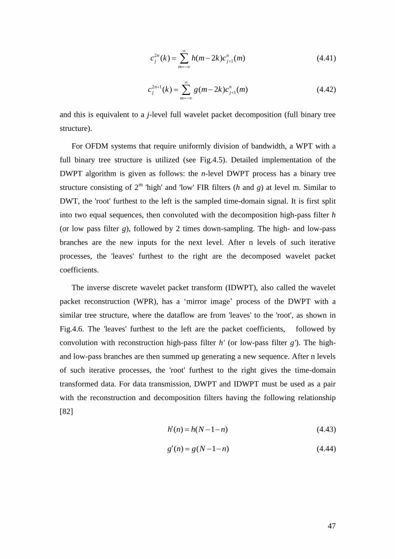
47
2
1( ) ( 2 ) ( )n n
j j
m
c k h m k c m
(4.41)
2 1
1( ) ( 2 ) ( )n n
j j
m
c k g m k c m
(4.42)
and this is equivalent to a j-level full wavelet packet decomposition (full binary tree
structure).
For OFDM systems that require uniformly division of bandwidth, a WPT with a
full binary tree structure is utilized (see Fig.4.5). Detailed implementation of the
DWPT algorithm is given as follows: the n-level DWPT process has a binary tree
structure consisting of 2m
'high' and 'low' FIR filters (h and g) at level m. Similar to
DWT, the 'root' furthest to the left is the sampled time-domain signal. It is first split
into two equal sequences, then convoluted with the decomposition high-pass filter h
(or low pass filter g), followed by 2 times down-sampling. The high- and low-pass
branches are the new inputs for the next level. After n levels of such iterative
processes, the 'leaves' furthest to the right are the decomposed wavelet packet
coefficients.
The inverse discrete wavelet packet transform (IDWPT), also called the wavelet
packet reconstruction (WPR), has a ‘mirror image’ process of the DWPT with a
similar tree structure, where the dataflow are from 'leaves' to the 'root', as shown in
Fig.4.6. The 'leaves' furthest to the left are the packet coefficients, followed by
convolution with reconstruction high-pass filter h' (or low-pass filter g'). The high-
and low-pass branches are then summed up generating a new sequence. After n levels
of such iterative processes, the 'root' furthest to the right gives the time-domain
transformed data. For data transmission, DWPT and IDWPT must be used as a pair
with the reconstruction and decomposition filters having the following relationship
[82]
( ) ( 1 )h n h N n (4.43)
( ) ( 1 )g n g N n (4.44)
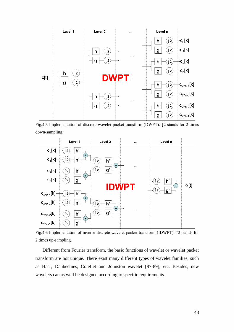
48
Fig.4.5 Implementation of discrete wavelet packet transform (DWPT). ↓2 stands for 2 times
down-sampling.
Fig.4.6 Implementation of inverse discrete wavelet packet transform (IDWPT). ↑2 stands for
2 times up-sampling.
Different from Fourier transform, the basic functions of wavelet or wavelet packet
transform are not unique. There exist many different types of wavelet families, such
as Haar, Daubechies, Coieflet and Johnston wavelet [87-89], etc. Besides, new
wavelets can as well be designed according to specific requirements.
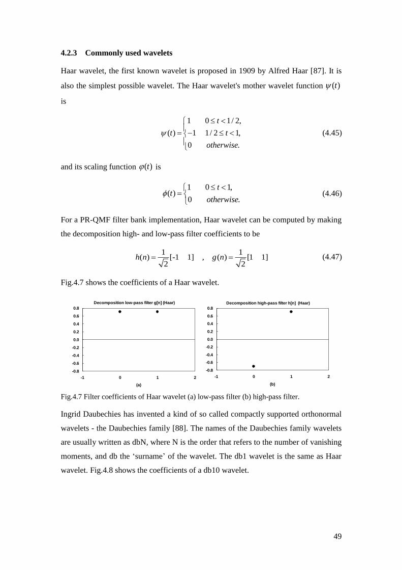
49
4.2.3 Commonly used wavelets
Haar wavelet, the first known wavelet is proposed in 1909 by Alfred Haar [87]. It is
also the simplest possible wavelet. The Haar wavelet's mother wavelet function ( )t
is
1 0 1/ 2,
( ) 1 1/ 2 1,
0 .
t
t t
otherwise
(4.45)
and its scaling function ( )t is
1 0 1,
( )0 .
tt
otherwise
(4.46)
For a PR-QMF filter bank implementation, Haar wavelet can be computed by making
the decomposition high- and low-pass filter coefficients to be
1 1
( ) [-1 1] , ( ) [1 1]2 2
h n g n (4.47)
Fig.4.7 shows the coefficients of a Haar wavelet.
Decomposition low-pass filter g[n] (Haar)
-0.8
-0.6
-0.4
-0.2
0.0
0.2
0.4
0.6
0.8
-1 0 1 2
(a)
Decomposition high-pass filter h[n] (Haar)
-0.8
-0.6
-0.4
-0.2
0.0
0.2
0.4
0.6
0.8
-1 0 1 2
(b)
Decomposition low-pass filter g[n] (Haar)
-0.8
-0.6
-0.4
-0.2
0.0
0.2
0.4
0.6
0.8
-1 0 1 2
(a)
Decomposition high-pass filter h[n] (Haar)
-0.8
-0.6
-0.4
-0.2
0.0
0.2
0.4
0.6
0.8
-1 0 1 2
(b)
Fig.4.7 Filter coefficients of Haar wavelet (a) low-pass filter (b) high-pass filter.
Ingrid Daubechies has invented a kind of so called compactly supported orthonormal
wavelets - the Daubechies family [88]. The names of the Daubechies family wavelets
are usually written as dbN, where N is the order that refers to the number of vanishing
moments, and db the ‘surname’ of the wavelet. The db1 wavelet is the same as Haar
wavelet. Fig.4.8 shows the coefficients of a db10 wavelet.
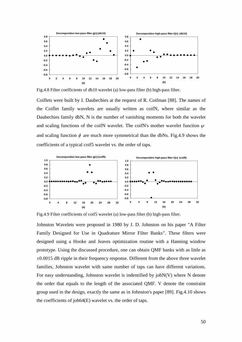
50
Decomposition low-pass filter g[n] (db10)
-0.8
-0.6
-0.4
-0.2
0.0
0.2
0.4
0.6
0.8
0 2 4 6 8 10 12 14 16 18 20
(a)
Decomposition high-pass filter h[n] (db10)
-0.8
-0.6
-0.4
-0.2
0.0
0.2
0.4
0.6
0.8
0 2 4 6 8 10 12 14 16 18 20
(b)
Decomposition low-pass filter g[n] (db10)
-0.8
-0.6
-0.4
-0.2
0.0
0.2
0.4
0.6
0.8
0 2 4 6 8 10 12 14 16 18 20
(a)
Decomposition high-pass filter h[n] (db10)
-0.8
-0.6
-0.4
-0.2
0.0
0.2
0.4
0.6
0.8
0 2 4 6 8 10 12 14 16 18 20
(b)
Fig.4.8 Filter coefficients of db10 wavelet (a) low-pass filter (b) high-pass filter.
Coiflets were built by I. Daubechies at the request of R. Coifman [88]. The names of
the Coiflet family wavelets are usually written as coifN, where similar as the
Daubechies family dbN, N is the number of vanishing moments for both the wavelet
and scaling functions of the coifN wavelet. The coifN's mother wavelet function
and scaling function are much more symmetrical than the dbNs. Fig.4.9 shows the
coefficients of a typical coif5 wavelet vs. the order of taps.
Decomposition low-pass filter g[n] (coif5)
-0.8
-0.6
-0.4
-0.2
0.0
0.2
0.4
0.6
0.8
1.0
0 4 8 12 16 20 24 28 32
(a)
Decomposition high-pass filter h[n] (coif5)
-0.8
-0.6
-0.4
-0.2
0.0
0.2
0.4
0.6
0.8
1.0
0 4 8 12 16 20 24 28 32
(b)
Decomposition low-pass filter g[n] (coif5)
-0.8
-0.6
-0.4
-0.2
0.0
0.2
0.4
0.6
0.8
1.0
0 4 8 12 16 20 24 28 32
(a)
Decomposition high-pass filter h[n] (coif5)
-0.8
-0.6
-0.4
-0.2
0.0
0.2
0.4
0.6
0.8
1.0
0 4 8 12 16 20 24 28 32
(b)
Fig.4.9 Filter coefficients of coif5 wavelet (a) low-pass filter (b) high-pass filter.
Johnston Wavelets were proposed in 1980 by J. D. Johnston on his paper "A Filter
Family Designed for Use in Quadrature Mirror Filter Banks". These filters were
designed using a Hooke and Jeaves optimization routine with a Hanning window
prototype. Using the discussed procedure, one can obtain QMF banks with as little as
±0.0015 dB ripple in their frequency response. Different from the above three wavelet
families, Johnston wavelet with same number of taps can have different variations.
For easy understanding, Johnston wavelet is indentified by johN(V) where N denote
the order that equals to the length of the associated QMF. V denote the constraint
group used in the design, exactly the same as in Johnston's paper [89]. Fig.4.10 shows
the coefficients of joh64(E) wavelet vs. the order of taps.
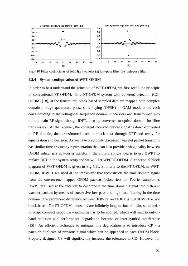
51
Decomposition low-pass filter g[n] (joh64(E))
-0.8
-0.6
-0.4
-0.2
0.0
0.2
0.4
0.6
0.8
0 8 16 24 32 40 48 56 64
(a)
Decomposition high-pass filter h[n] (joh64(E))
-0.8
-0.6
-0.4
-0.2
0.0
0.2
0.4
0.6
0.8
0 8 16 24 32 40 48 56 64
(b)
Fig.4.10 Filter coefficients of joh64(E) wavelet (a) low-pass filter (b) high-pass filter.
4.2.4 System configuration of WPT-OFDM
In order to best understand the principle of WPT-OFDM, we first recall the principle
of conventional FT-OFDM. In a FT-OFDM system with coherent detection (CO-
OFDM) [18], at the transmitter, block based sampled data are mapped onto complex
domain through quadrature phase shift keying (QPSK) or QAM modulation, each
corresponding to the orthogonal frequency domain subcarriers and transformed into
time domain RF signal though IDFT, then up-converted to optical domain for fibre
transmission. At the receiver, the coherent received optical signal is down-converted
to RF domain, then transformed back to block data through DFT and ready for
equalization and decision. As we have previously discussed, wavelet packet transform
has similar time-frequency representation that can also provide orthogonality between
OFDM subcarriers as Fourier transform, therefore a simple idea is to use DWPT to
replace DFT in the system setup and we will get WP(F)T-OFDM. A conceptual block
diagram of WPT-OFDM is given in Fig.4.11. Similarly to the FT-OFDM, in WPT-
OFDM, IDWPT are used at the transmitter that reconstructs the time domain signal
from the one-on-one mapped OFDM packets (subcarriers for Fourier transform).
DWPT are used at the receiver to decompose the time domain signal into different
wavelet packets by means of successive low-pass and high-pass filtering in the time
domain. The prominent difference between IDWPT and IDFT is that IDWPT is not
block based. For FT-OFDM, sinusoids are infinitely long in time domain, so in order
to adapt compact support a windowing has to be applied, which will lead to out-of-
band radiation and performance degradation because of inter-symbol interference
(ISI). An efficient technique to mitigate this degradation is to introduce CP - a
partition duplicate of previous signal which can be appended to each OFDM block.
Properly designed CP will significantly increase the tolerance to CD. However for
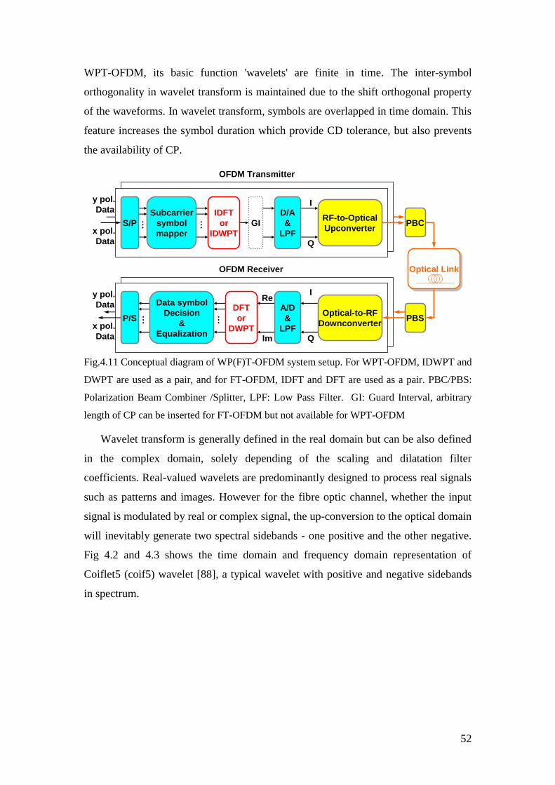
52
WPT-OFDM, its basic function 'wavelets' are finite in time. The inter-symbol
orthogonality in wavelet transform is maintained due to the shift orthogonal property
of the waveforms. In wavelet transform, symbols are overlapped in time domain. This
feature increases the symbol duration which provide CD tolerance, but also prevents
the availability of CP.
x pol.
Data
I
Q
OFDM Transmitter
Optical LinkOptical Link
…
… …
Re
Im
x pol.
Data
…
IDFT
or
IDWPT
Subcarrier
symbol
mapper
S/P
D/A
&
LPF
GIRF-to-Optical
Upconverter
DFT
or
DWPT
Data symbol
Decision
&
Equalization
P/S
OFDM Receiver
y pol.
Data
y pol.
Data
PBC
PBS
I
Q
A/D
&
LPF
Optical-to-RF
Downconverter
Fig.4.11 Conceptual diagram of WP(F)T-OFDM system setup. For WPT-OFDM, IDWPT and
DWPT are used as a pair, and for FT-OFDM, IDFT and DFT are used as a pair. PBC/PBS:
Polarization Beam Combiner /Splitter, LPF: Low Pass Filter. GI: Guard Interval, arbitrary
length of CP can be inserted for FT-OFDM but not available for WPT-OFDM
Wavelet transform is generally defined in the real domain but can be also defined
in the complex domain, solely depending of the scaling and dilatation filter
coefficients. Real-valued wavelets are predominantly designed to process real signals
such as patterns and images. However for the fibre optic channel, whether the input
signal is modulated by real or complex signal, the up-conversion to the optical domain
will inevitably generate two spectral sidebands - one positive and the other negative.
Fig 4.2 and 4.3 shows the time domain and frequency domain representation of
Coiflet5 (coif5) wavelet [88], a typical wavelet with positive and negative sidebands
in spectrum.
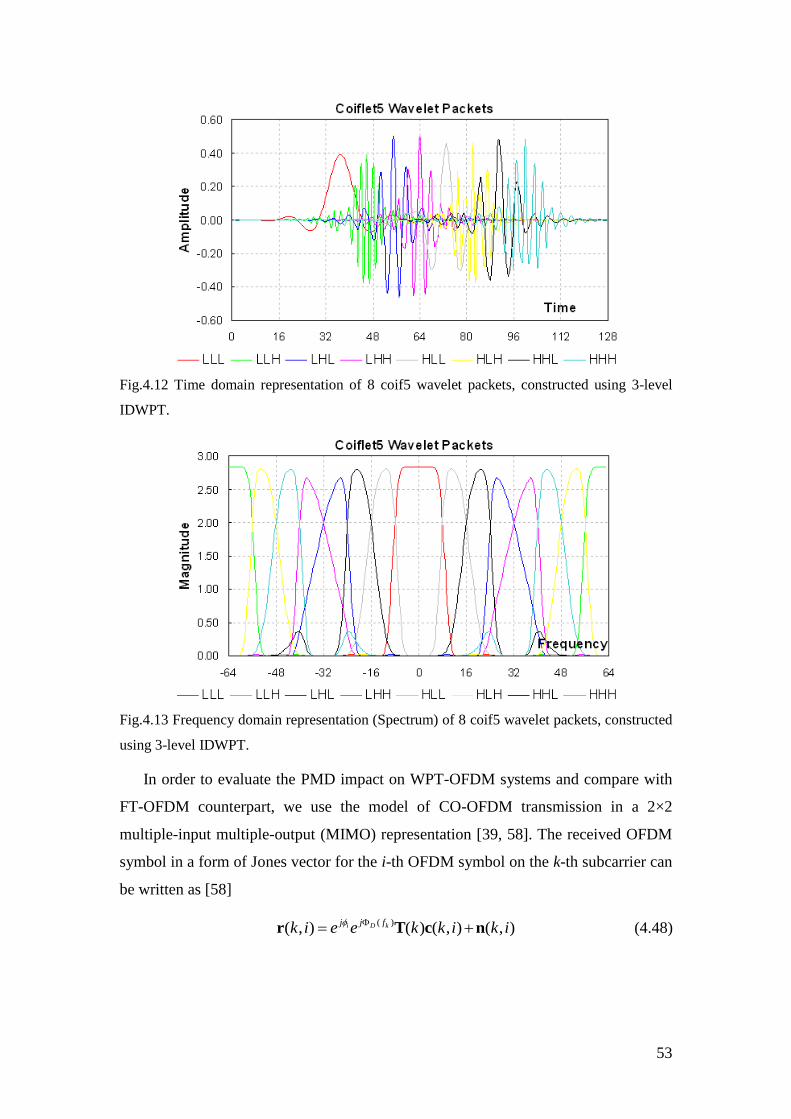
53
Fig.4.12 Time domain representation of 8 coif5 wavelet packets, constructed using 3-level
IDWPT.
Fig.4.13 Frequency domain representation (Spectrum) of 8 coif5 wavelet packets, constructed
using 3-level IDWPT.
In order to evaluate the PMD impact on WPT-OFDM systems and compare with
FT-OFDM counterpart, we use the model of CO-OFDM transmission in a 2×2
multiple-input multiple-output (MIMO) representation [39, 58]. The received OFDM
symbol in a form of Jones vector for the i-th OFDM symbol on the k-th subcarrier can
be written as [58]
( )
( , ) ( ) ( , ) ( , )i D kj j fk i e e k k i k i
r T c n (4.48)
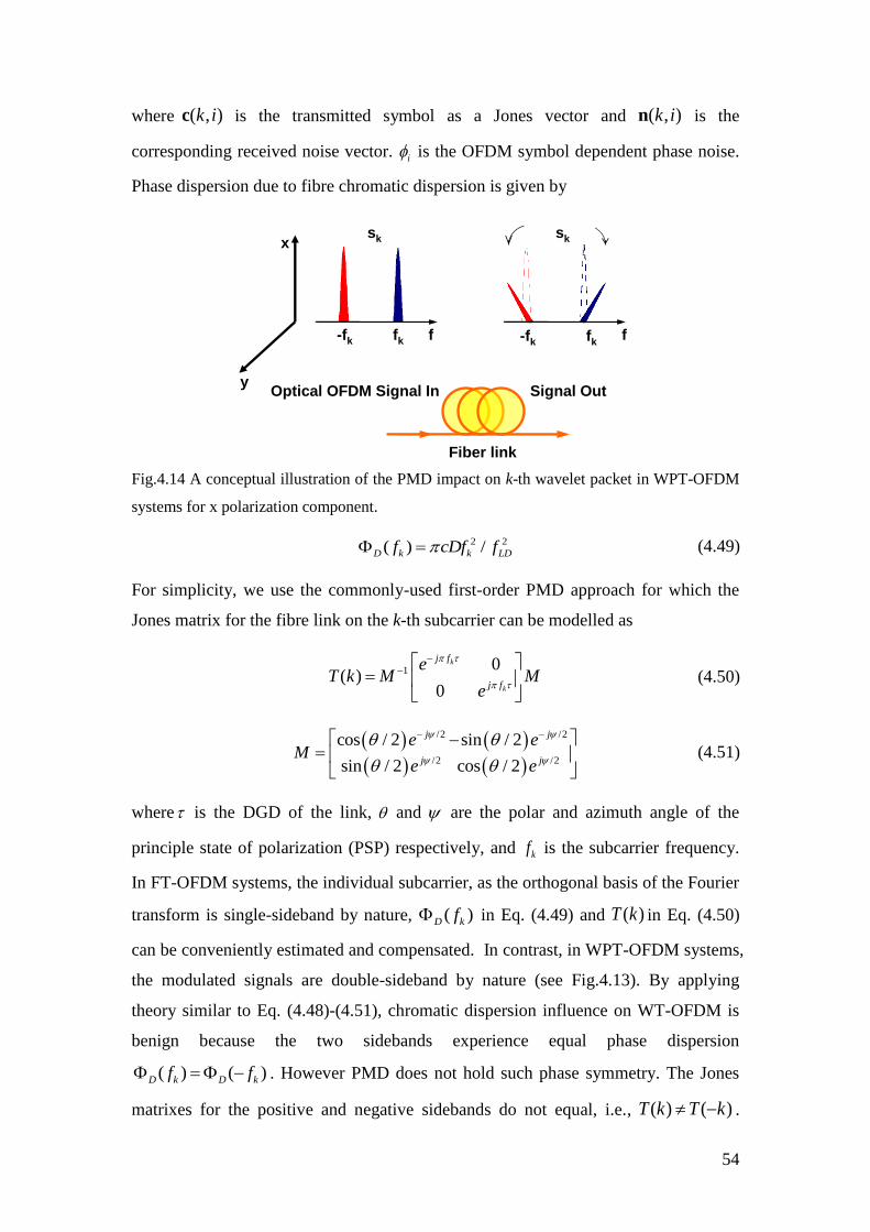
54
where ( , )k ic is the transmitted symbol as a Jones vector and ( , )k in is the
corresponding received noise vector. i is the OFDM symbol dependent phase noise.
Phase dispersion due to fibre chromatic dispersion is given by
Optical OFDM Signal In
-fk fk
x
y
Fiber link
Signal Out
sk
f
si
f-fk fk
sk
Fig.4.14 A conceptual illustration of the PMD impact on k-th wavelet packet in WPT-OFDM
systems for x polarization component.
2 2( ) /D k k LDf cDf f (4.49)
For simplicity, we use the commonly-used first-order PMD approach for which the
Jones matrix for the fibre link on the k-th subcarrier can be modelled as
1 0
( )0
k
k
j f
j f
eT k M M
e
(4.50)
/2 /2
/2 /2
cos / 2 sin / 2
sin / 2 cos / 2
j j
j j
e eM
e e
(4.51)
where is the DGD of the link, and are the polar and azimuth angle of the
principle state of polarization (PSP) respectively, and kf is the subcarrier frequency.
In FT-OFDM systems, the individual subcarrier, as the orthogonal basis of the Fourier
transform is single-sideband by nature, ( )D kf in Eq. (4.49) and ( )T k in Eq. (4.50)
can be conveniently estimated and compensated. In contrast, in WPT-OFDM systems,
the modulated signals are double-sideband by nature (see Fig.4.13). By applying
theory similar to Eq. (4.48)-(4.51), chromatic dispersion influence on WT-OFDM is
benign because the two sidebands experience equal phase dispersion
( ) ( )D k D kf f . However PMD does not hold such phase symmetry. The Jones
matrixes for the positive and negative sidebands do not equal, i.e., ( ) ( )T k T k .
55
Upon reception where the two sidebands need to be recombined and projected onto
real wavelet basis, the two sidebands experience two different dispersions, and the
addition of the two does not reproduce the real-wavelet basis, resulting in violation of
the orthogonality and therefore inter-packet-interference. This is illustrated in Fig.4.14
where the conceptual figure of PMD impact on OFDM subcarriers in one polarization
launch is shown. We conclude that WPT-OFDM will be more susceptible to PMD
than conventional FT-OFDM.
A similar one-tap equalizer [39, 58, 132-134] is utilized to equalize both CD and
PMD impact in WPT-OFDM. The channel matrix H is estimated by sending OFDM
symbols using alternative polarization launch. Mathematically, the transmitter
information symbol of the two polarizations and fibre response in the forms of Jones
vector are given by
1 11 12
2 21 22
,c h h
c Hc h h
(4.52)
The received symbol is given by
1
2
cc H c
c
(4.53)
Using odd training symbols, the associated channel estimation can be expressed as
1 11 12 11 1 11
2 21 22 21 2 1
/
/0
c h h h c cc
c h h h c c
(4.54)
And using even symbols,
1 11 12 12 1 2
22 21 22 22 2 2
/0
/
c h h h c c
cc h h h c c
(4.55)
4.2.5 Simulation and results
We have carried out numerical simulation to compare the transmission performance
of dual-polarization WPT-OFDM systems with FT-OFDM systems. The simulation
parameters are shown in Table 4.1: Dual-polarization OFDM data rate at 112 Gb/s,
the number of subcarriers varying from 64 to 256. The number of symbols in FT-
OFDM is 256 and for WPT-OFDM we maintain the same total length as in FT-
OFDM. We have three choices of oversampling, no oversampling, oversampled by
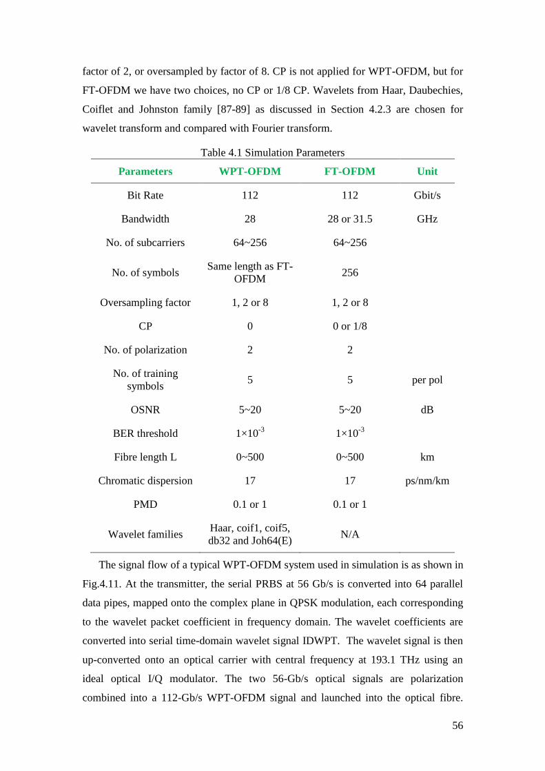
56
factor of 2, or oversampled by factor of 8. CP is not applied for WPT-OFDM, but for
FT-OFDM we have two choices, no CP or 1/8 CP. Wavelets from Haar, Daubechies,
Coiflet and Johnston family [87-89] as discussed in Section 4.2.3 are chosen for
wavelet transform and compared with Fourier transform.
Table 4.1 Simulation Parameters
Parameters WPT-OFDM FT-OFDM Unit
Bit Rate 112 112 Gbit/s
Bandwidth 28 28 or 31.5 GHz
No. of subcarriers 64~256 64~256
No. of symbols Same length as FT-
OFDM 256
Oversampling factor 1, 2 or 8 1, 2 or 8
CP 0 0 or 1/8
No. of polarization 2 2
No. of training
symbols 5 5 per pol
OSNR 5~20 5~20 dB
BER threshold 1×10⁻³
1×10⁻³
Fibre length L 0~500 0~500 km
Chromatic dispersion 17 17 ps/nm/km
PMD 0.1 or 1 0.1 or 1
Wavelet families Haar, coif1, coif5,
db32 and Joh64(E) N/A
The signal flow of a typical WPT-OFDM system used in simulation is as shown in
Fig.4.11. At the transmitter, the serial PRBS at 56 Gb/s is converted into 64 parallel
data pipes, mapped onto the complex plane in QPSK modulation, each corresponding
to the wavelet packet coefficient in frequency domain. The wavelet coefficients are
converted into serial time-domain wavelet signal IDWPT. The wavelet signal is then
up-converted onto an optical carrier with central frequency at 193.1 THz using an
ideal optical I/Q modulator. The two 56-Gb/s optical signals are polarization
combined into a 112-Gb/s WPT-OFDM signal and launched into the optical fibre.
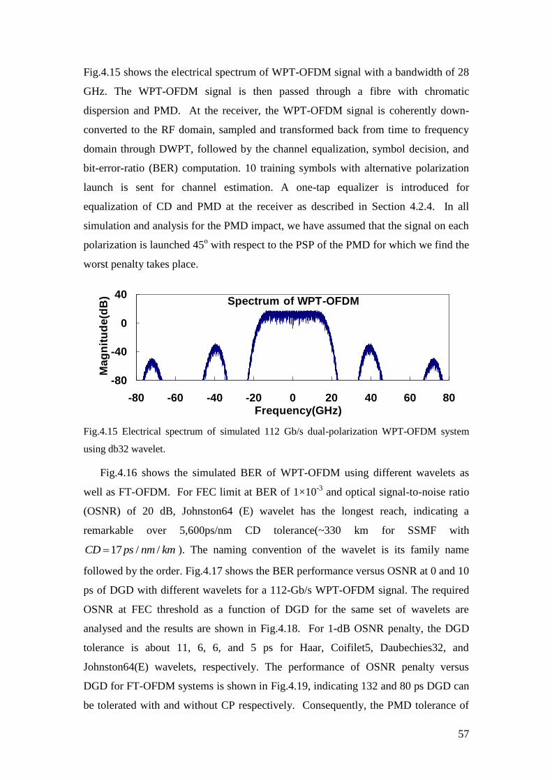
57
Fig.4.15 shows the electrical spectrum of WPT-OFDM signal with a bandwidth of 28
GHz. The WPT-OFDM signal is then passed through a fibre with chromatic
dispersion and PMD. At the receiver, the WPT-OFDM signal is coherently down-
converted to the RF domain, sampled and transformed back from time to frequency
domain through DWPT, followed by the channel equalization, symbol decision, and
bit-error-ratio (BER) computation. 10 training symbols with alternative polarization
launch is sent for channel estimation. A one-tap equalizer is introduced for
equalization of CD and PMD at the receiver as described in Section 4.2.4. In all
simulation and analysis for the PMD impact, we have assumed that the signal on each
polarization is launched 45o with respect to the PSP of the PMD for which we find the
worst penalty takes place.
Spectrum of WPT-OFDM
-80
-40
0
40
-80 -60 -40 -20 0 20 40 60 80Frequency(GHz)
Mag
nit
ud
e(d
B)
Fig.4.15 Electrical spectrum of simulated 112 Gb/s dual-polarization WPT-OFDM system
using db32 wavelet.
Fig.4.16 shows the simulated BER of WPT-OFDM using different wavelets as
well as FT-OFDM. For FEC limit at BER of 1×10⁻³
and optical signal-to-noise ratio
(OSNR) of 20 dB, Johnston64 (E) wavelet has the longest reach, indicating a
remarkable over 5,600ps/nm CD tolerance(~330 km for SSMF with
17 / /CD ps nm km ). The naming convention of the wavelet is its family name
followed by the order. Fig.4.17 shows the BER performance versus OSNR at 0 and 10
ps of DGD with different wavelets for a 112-Gb/s WPT-OFDM signal. The required
OSNR at FEC threshold as a function of DGD for the same set of wavelets are
analysed and the results are shown in Fig.4.18. For 1-dB OSNR penalty, the DGD
tolerance is about 11, 6, 6, and 5 ps for Haar, Coifilet5, Daubechies32, and
Johnston64(E) wavelets, respectively. The performance of OSNR penalty versus
DGD for FT-OFDM systems is shown in Fig.4.19, indicating 132 and 80 ps DGD can
be tolerated with and without CP respectively. Consequently, the PMD tolerance of
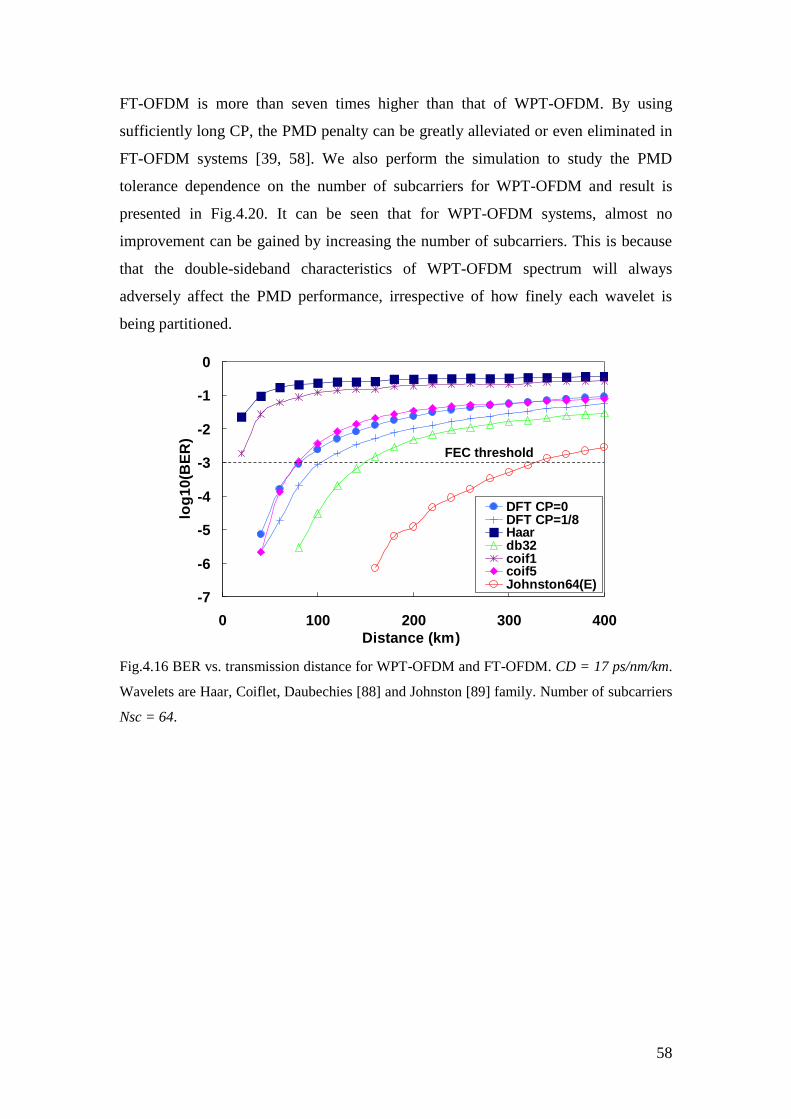
58
FT-OFDM is more than seven times higher than that of WPT-OFDM. By using
sufficiently long CP, the PMD penalty can be greatly alleviated or even eliminated in
FT-OFDM systems [39, 58]. We also perform the simulation to study the PMD
tolerance dependence on the number of subcarriers for WPT-OFDM and result is
presented in Fig.4.20. It can be seen that for WPT-OFDM systems, almost no
improvement can be gained by increasing the number of subcarriers. This is because
that the double-sideband characteristics of WPT-OFDM spectrum will always
adversely affect the PMD performance, irrespective of how finely each wavelet is
being partitioned.
-7
-6
-5
-4
-3
-2
-1
0
0 100 200 300 400
Distance (km)
log
10
(BE
R)
DFT CP=0DFT CP=1/8Haardb32coif1coif5Johnston64(E)
FEC threshold
Fig.4.16 BER vs. transmission distance for WPT-OFDM and FT-OFDM. CD = 17 ps/nm/km.
Wavelets are Haar, Coiflet, Daubechies [88] and Johnston [89] family. Number of subcarriers
Nsc = 64.

59
Wavelet DGD(ps)
-6
-5
-4
-3
-2
-1
10 12 14 16 18 20OSNR (dB)
log
10
(BE
R)
Haar 0Haar 10coif5 0coif5 10db32 0db32 10Johnston64(E) 0Johnston64(E) 10
Fig.4.17 BER vs. OSNR for WPT-OFDM without DGD (0ps) and with DGD (10ps). Nsc =
64.
14
16
18
20
22
24
26
28
30
0 1 2 3 4 5 6 7 8 9 10DGD(ps)
Req
uir
ed
OS
NR
(dB
)
Haarcoif5
db32Johnston64(E)
Fig.4.18 Required OSNR at BER=1×10
-3 vs. DGD for WPT-OFDM. Nsc = 64.
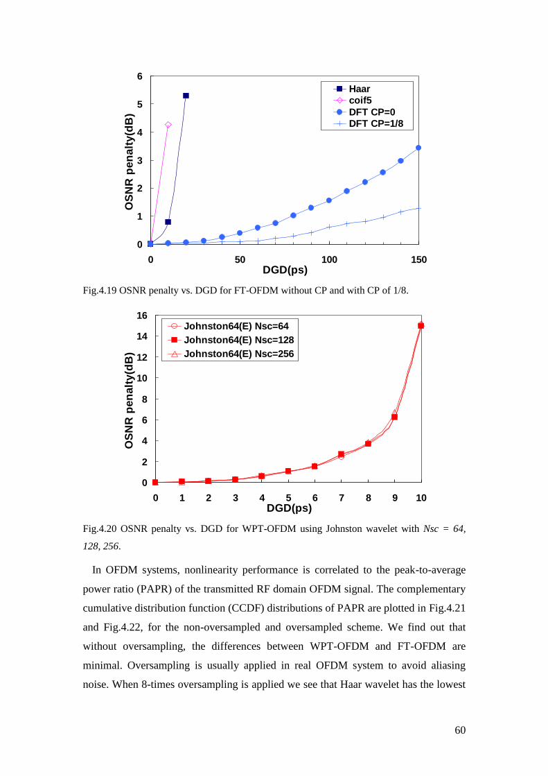
60
0
1
2
3
4
5
6
0 50 100 150DGD(ps)
OS
NR
pen
alt
y(d
B)
Haarcoif5
DFT CP=0DFT CP=1/8
Fig.4.19 OSNR penalty vs. DGD for FT-OFDM without CP and with CP of 1/8.
0
2
4
6
8
10
12
14
16
0 1 2 3 4 5 6 7 8 9 10DGD(ps)
OS
NR
pe
na
lty
(dB
)
Johnston64(E) Nsc=64
Johnston64(E) Nsc=128
Johnston64(E) Nsc=256
Fig.4.20 OSNR penalty vs. DGD for WPT-OFDM using Johnston wavelet with Nsc = 64,
128, 256.
In OFDM systems, nonlinearity performance is correlated to the peak-to-average
power ratio (PAPR) of the transmitted RF domain OFDM signal. The complementary
cumulative distribution function (CCDF) distributions of PAPR are plotted in Fig.4.21
and Fig.4.22, for the non-oversampled and oversampled scheme. We find out that
without oversampling, the differences between WPT-OFDM and FT-OFDM are
minimal. Oversampling is usually applied in real OFDM system to avoid aliasing
noise. When 8-times oversampling is applied we see that Haar wavelet has the lowest
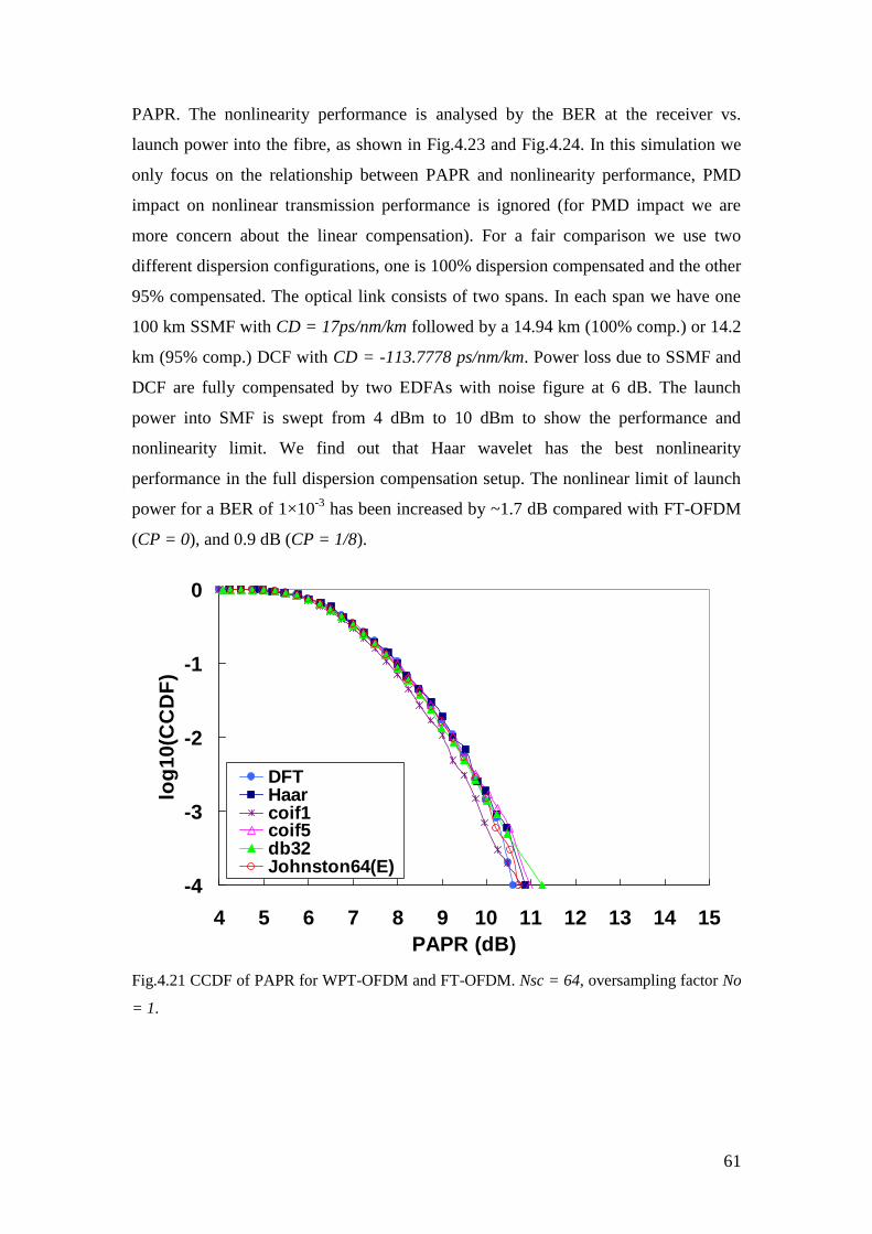
61
PAPR. The nonlinearity performance is analysed by the BER at the receiver vs.
launch power into the fibre, as shown in Fig.4.23 and Fig.4.24. In this simulation we
only focus on the relationship between PAPR and nonlinearity performance, PMD
impact on nonlinear transmission performance is ignored (for PMD impact we are
more concern about the linear compensation). For a fair comparison we use two
different dispersion configurations, one is 100% dispersion compensated and the other
95% compensated. The optical link consists of two spans. In each span we have one
100 km SSMF with CD = 17ps/nm/km followed by a 14.94 km (100% comp.) or 14.2
km (95% comp.) DCF with CD = -113.7778 ps/nm/km. Power loss due to SSMF and
DCF are fully compensated by two EDFAs with noise figure at 6 dB. The launch
power into SMF is swept from 4 dBm to 10 dBm to show the performance and
nonlinearity limit. We find out that Haar wavelet has the best nonlinearity
performance in the full dispersion compensation setup. The nonlinear limit of launch
power for a BER of 1×10⁻³
has been increased by ~1.7 dB compared with FT-OFDM
(CP = 0), and 0.9 dB (CP = 1/8).
-4
-3
-2
-1
0
4 5 6 7 8 9 10 11 12 13 14 15
PAPR (dB)
log
10
(CC
DF
)
DFTHaarcoif1coif5db32Johnston64(E)
Fig.4.21 CCDF of PAPR for WPT-OFDM and FT-OFDM. Nsc = 64, oversampling factor No
= 1.
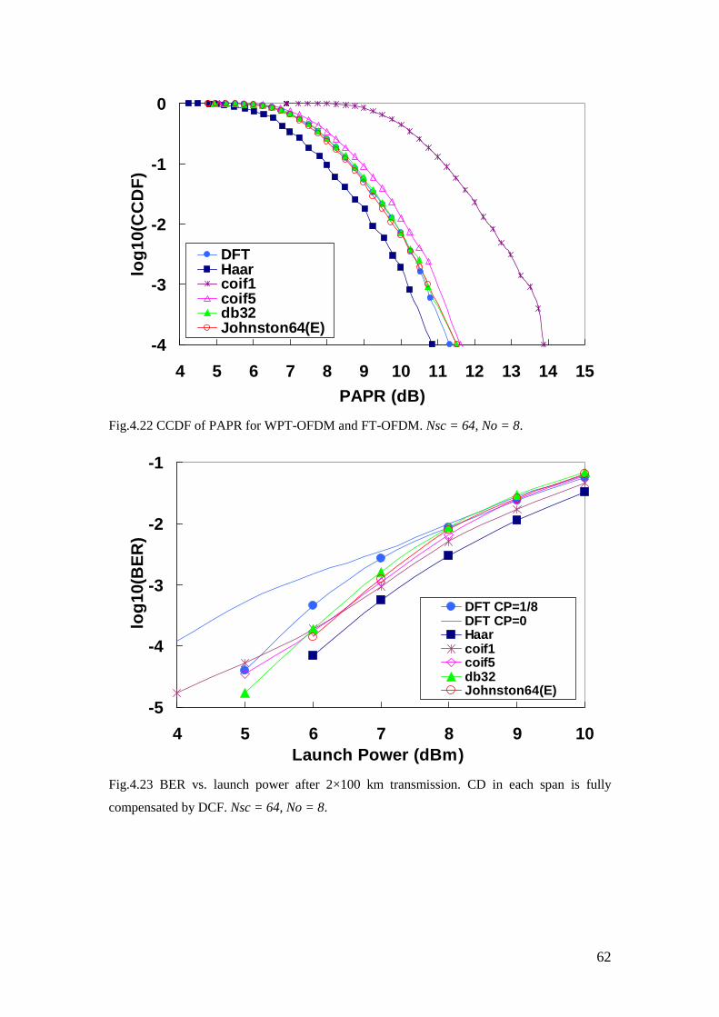
62
-4
-3
-2
-1
0
4 5 6 7 8 9 10 11 12 13 14 15
PAPR (dB)
log
10
(CC
DF
)
DFTHaarcoif1coif5db32Johnston64(E)
Fig.4.22 CCDF of PAPR for WPT-OFDM and FT-OFDM. Nsc = 64, No = 8.
-5
-4
-3
-2
-1
4 5 6 7 8 9 10
Launch Power (dBm)
log
10
(BE
R)
DFT CP=1/8DFT CP=0Haarcoif1coif5db32Johnston64(E)
Fig.4.23 BER vs. launch power after 2×100 km transmission. CD in each span is fully
compensated by DCF. Nsc = 64, No = 8.
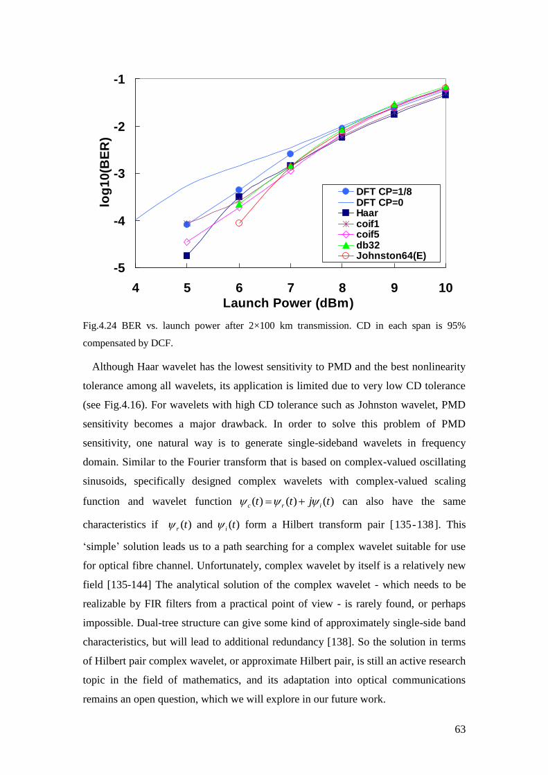
63
-5
-4
-3
-2
-1
4 5 6 7 8 9 10
Launch Power (dBm)
log
10
(BE
R)
DFT CP=1/8DFT CP=0Haarcoif1coif5db32Johnston64(E)
Fig.4.24 BER vs. launch power after 2×100 km transmission. CD in each span is 95%
compensated by DCF.
Although Haar wavelet has the lowest sensitivity to PMD and the best nonlinearity
tolerance among all wavelets, its application is limited due to very low CD tolerance
(see Fig.4.16). For wavelets with high CD tolerance such as Johnston wavelet, PMD
sensitivity becomes a major drawback. In order to solve this problem of PMD
sensitivity, one natural way is to generate single-sideband wavelets in frequency
domain. Similar to the Fourier transform that is based on complex-valued oscillating
sinusoids, specifically designed complex wavelets with complex-valued scaling
function and wavelet function ( ) ( ) ( )c r it t j t can also have the same
characteristics if ( )r t and ( ) i t form a Hilbert transform pair [135-138]. This
‘simple’ solution leads us to a path searching for a complex wavelet suitable for use
for optical fibre channel. Unfortunately, complex wavelet by itself is a relatively new
field [135-144] The analytical solution of the complex wavelet - which needs to be
realizable by FIR filters from a practical point of view - is rarely found, or perhaps
impossible. Dual-tree structure can give some kind of approximately single-side band
characteristics, but will lead to additional redundancy [138]. So the solution in terms
of Hilbert pair complex wavelet, or approximate Hilbert pair, is still an active research
topic in the field of mathematics, and its adaptation into optical communications
remains an open question, which we will explore in our future work.
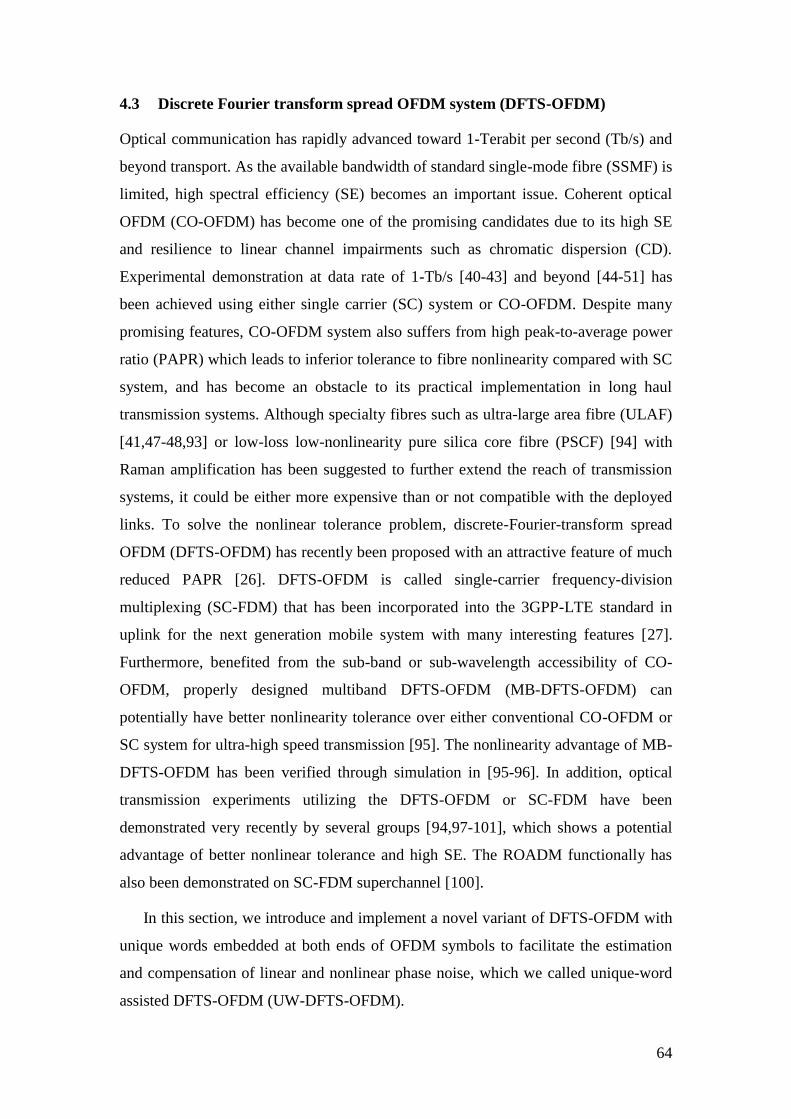
64
4.3 Discrete Fourier transform spread OFDM system (DFTS-OFDM)
Optical communication has rapidly advanced toward 1-Terabit per second (Tb/s) and
beyond transport. As the available bandwidth of standard single-mode fibre (SSMF) is
limited, high spectral efficiency (SE) becomes an important issue. Coherent optical
OFDM (CO-OFDM) has become one of the promising candidates due to its high SE
and resilience to linear channel impairments such as chromatic dispersion (CD).
Experimental demonstration at data rate of 1-Tb/s [40-43] and beyond [44-51] has
been achieved using either single carrier (SC) system or CO-OFDM. Despite many
promising features, CO-OFDM system also suffers from high peak-to-average power
ratio (PAPR) which leads to inferior tolerance to fibre nonlinearity compared with SC
system, and has become an obstacle to its practical implementation in long haul
transmission systems. Although specialty fibres such as ultra-large area fibre (ULAF)
[41,47-48,93] or low-loss low-nonlinearity pure silica core fibre (PSCF) [94] with
Raman amplification has been suggested to further extend the reach of transmission
systems, it could be either more expensive than or not compatible with the deployed
links. To solve the nonlinear tolerance problem, discrete-Fourier-transform spread
OFDM (DFTS-OFDM) has recently been proposed with an attractive feature of much
reduced PAPR [26]. DFTS-OFDM is called single-carrier frequency-division
multiplexing (SC-FDM) that has been incorporated into the 3GPP-LTE standard in
uplink for the next generation mobile system with many interesting features [27].
Furthermore, benefited from the sub-band or sub-wavelength accessibility of CO-
OFDM, properly designed multiband DFTS-OFDM (MB-DFTS-OFDM) can
potentially have better nonlinearity tolerance over either conventional CO-OFDM or
SC system for ultra-high speed transmission [95]. The nonlinearity advantage of MB-
DFTS-OFDM has been verified through simulation in [95-96]. In addition, optical
transmission experiments utilizing the DFTS-OFDM or SC-FDM have been
demonstrated very recently by several groups [94,97-101], which shows a potential
advantage of better nonlinear tolerance and high SE. The ROADM functionally has
also been demonstrated on SC-FDM superchannel [100].
In this section, we introduce and implement a novel variant of DFTS-OFDM with
unique words embedded at both ends of OFDM symbols to facilitate the estimation
and compensation of linear and nonlinear phase noise, which we called unique-word
assisted DFTS-OFDM (UW-DFTS-OFDM).
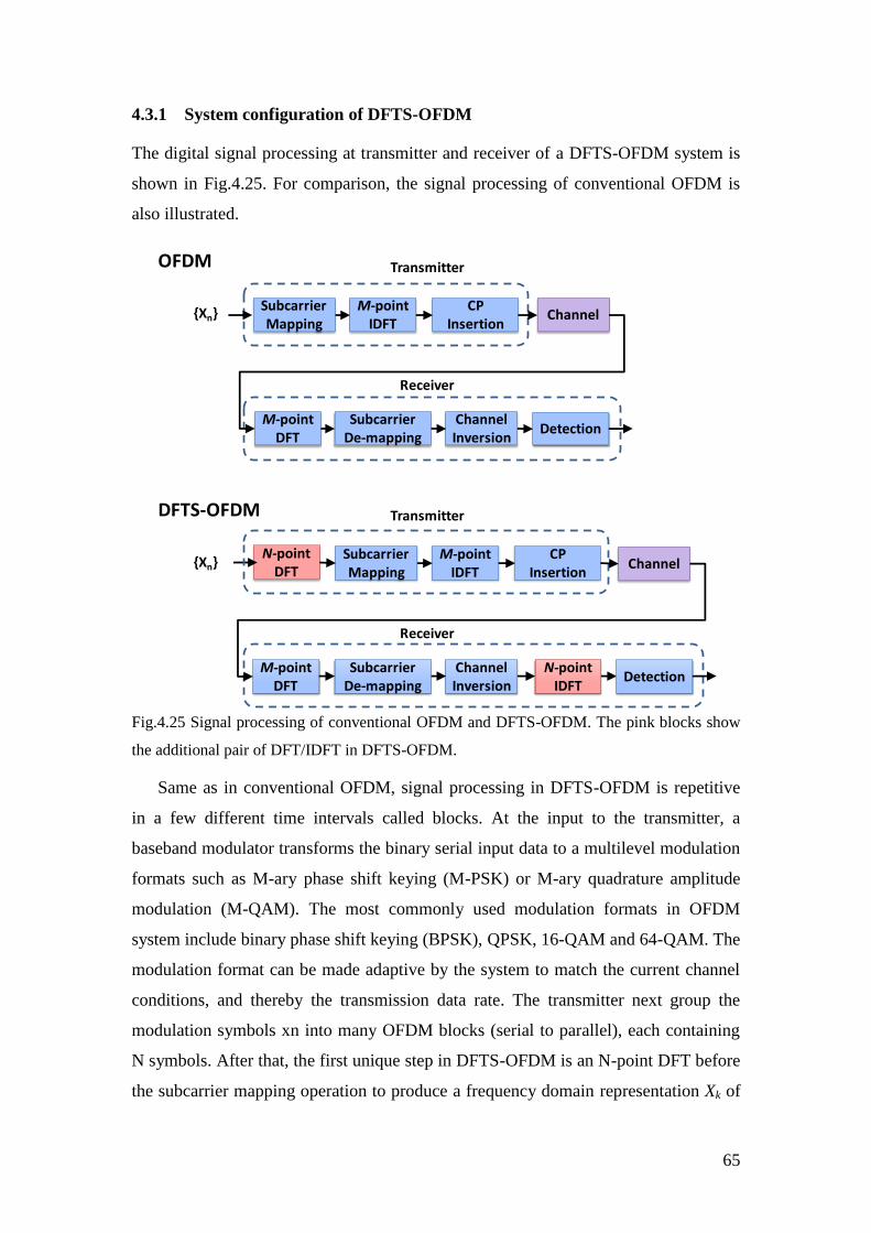
65
4.3.1 System configuration of DFTS-OFDM
The digital signal processing at transmitter and receiver of a DFTS-OFDM system is
shown in Fig.4.25. For comparison, the signal processing of conventional OFDM is
also illustrated.
M-pointIDFT
CPInsertion
Channel
M-pointDFT
Channel Inversion
Detection
OFDM
DFTS-OFDM
M-pointDFT
Channel Inversion
N-pointDFT
N-pointIDFT
Transmitter
Receiver
Transmitter
Receiver
SubcarrierMapping
SubcarrierDe-mapping
M-pointIDFT
CPInsertion
ChannelSubcarrierMapping
DetectionSubcarrier
De-mapping
{Xn}
{Xn}
Fig.4.25 Signal processing of conventional OFDM and DFTS-OFDM. The pink blocks show
the additional pair of DFT/IDFT in DFTS-OFDM.
Same as in conventional OFDM, signal processing in DFTS-OFDM is repetitive
in a few different time intervals called blocks. At the input to the transmitter, a
baseband modulator transforms the binary serial input data to a multilevel modulation
formats such as M-ary phase shift keying (M-PSK) or M-ary quadrature amplitude
modulation (M-QAM). The most commonly used modulation formats in OFDM
system include binary phase shift keying (BPSK), QPSK, 16-QAM and 64-QAM. The
modulation format can be made adaptive by the system to match the current channel
conditions, and thereby the transmission data rate. The transmitter next group the
modulation symbols xn into many OFDM blocks (serial to parallel), each containing
N symbols. After that, the first unique step in DFTS-OFDM is an N-point DFT before
the subcarrier mapping operation to produce a frequency domain representation Xk of
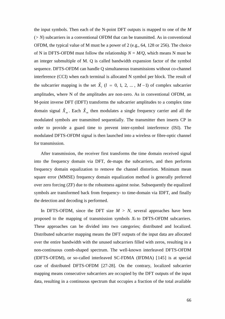
66
the input symbols. Then each of the N-point DFT outputs is mapped to one of the M
(> N) subcarriers in a conventional OFDM that can be transmitted. As in conventional
OFDM, the typical value of M must be a power of 2 (e.g., 64, 128 or 256). The choice
of N in DFTS-OFDM must follow the relationship N = M/Q, which means N must be
an integer submultiple of M. Q is called bandwidth expansion factor of the symbol
sequence. DFTS-OFDM can handle Q simultaneous transmissions without co-channel
interference (CCI) when each terminal is allocated N symbol per block. The result of
the subcarrier mapping is the set ( 0, 1, 2, ... , 1)lX l M of complex subcarrier
amplitudes, where N of the amplitudes are non-zero. As in conventional OFDM, an
M-point inverse DFT (IDFT) transforms the subcarrier amplitudes to a complex time
domain signal mX . Each mX then modulates a single frequency carrier and all the
modulated symbols are transmitted sequentially. The transmitter then inserts CP in
order to provide a guard time to prevent inter-symbol interference (ISI). The
modulated DFTS-OFDM signal is then launched into a wireless or fibre-optic channel
for transmission.
After transmission, the receiver first transforms the time domain received signal
into the frequency domain via DFT, de-maps the subcarriers, and then performs
frequency domain equalization to remove the channel distortion. Minimum mean
square error (MMSE) frequency domain equalization method is generally preferred
over zero forcing (ZF) due to the robustness against noise. Subsequently the equalized
symbols are transformed back from frequency- to time-domain via IDFT, and finally
the detection and decoding is performed.
In DFTS-OFDM, since the DFT size M > N, several approaches have been
proposed to the mapping of transmission symbols Xk to DFTS-OFDM subcarriers.
These approaches can be divided into two categories; distributed and localized.
Distributed subcarrier mapping means the DFT outputs of the input data are allocated
over the entire bandwidth with the unused subcarriers filled with zeros, resulting in a
non-continuous comb-shaped spectrum. The well-known interleaved DFTS-OFDM
(IDFTS-OFDM), or so-called interleaved SC-FDMA (IFDMA) [145] is at special
case of distributed DFTS-OFDM [27-28]. On the contrary, localized subcarrier
mapping means consecutive subcarriers are occupied by the DFT outputs of the input
data, resulting in a continuous spectrum that occupies a fraction of the total available

67
bandwidth. For IDFTS-OFDM, time symbols are simply a repetition of the original
input symbols with a systematic phase rotation applied to each symbol in the time
domain [145]. Therefore, the PAPR of IDFTS-OFDM signal is the same as in the case
of a conventional single carrier signal. In the case of localized DFTS-OFDM
(LDFTS-OFDM), or so-called localized SC-FDMA (LFDMA), the time signal has
exact copies of input time symbols in N sample positions. The other M-N time
samples are weighted sums of all the symbols in the input block [146]. As we can see
from Fig.4.25, the first and obvious difference between conventional OFDM and
DFTS-OFDM is the additional pair of N-point DFT/IDFT (pink blocks in Fig.4.25) in
the DFTS-OFDM, with DFT in the transmitter and IDFT in the receiver. The second
fundamental difference between DFTS-OFDM and conventional OFDM is in the
receiver equalization and detection processes [28]. In conventional OFDM, since the
data symbol is carried by individual subcarriers, channel equalization, channel
inversion and data detection is performed individually on each subcarrier [16].
Channel coding or power/rate adaptation is required for OFDM to protect individual
subcarriers if there are nulls in the channel spectrum, which would severely degrade
the system performance since there is essentially no way to recover the data affected
by the null. In the case of DFTS-OFDM, channel equalization and inversion is done
similarly in the frequency domain but data detection is performed after the frequency
domain equalized data is reverted back to time domain by IDFT [28]. Hence, it is
more robust to spectral nulls compared to conventional OFDM since the noise is
averaged out over the entire bandwidth. Additional advantages of DFTS-OFDM are
the less sensitivity to carrier frequency offset (CFO) and less nonlinear distortion due
to the much reduced PAPR [26], whilst conventional OFDM suffers due to the
multicarrier nature of OFDM [147].
4.3.2 Principle of unique word DFTS-OFDM (UW-DFTS-OFDM)
Unique-word (UW) was first proposed for single carrier frequency domain
equalization (SC-FDE) systems and has been extensively studied in wireless
communications [145-150]. The data pattern structure of UW-DFTS-OFDM for two
polarizations is illustrated in Fig.4.26. The unique-words (UWs), normally comprising
of a Zadoff-Chu (ZC) sequence [151] and an optional guard interval (GI) are inserted
periodically at the both ends of payload. The Zadoff-Chu sequence is generated with
the following equation
68
2
1
(0 1)ZC
ZC
un nj
N
ZC
u ZCun
jN
ZC
e if N is oddx n n N
e if N is even
(4.56)
where ( )ux n is the Zadoff-Chu sequence, Nzc is sequence length, u is an integer
relatively prime of Nzc. A similar OFDM symbol structure can be drawn for the
second polarization by using different UWs. The reason to use two UWs within one
OFDM symbol is compatibility with polarization diversity where the first and second
UWs are orthogonal to each other when combining the two OFDM symbols for two
polarizations in a Jones vector form. The two UWs for the two polarizations (see
Fig.4.26), 1
1
x
y
UW
UW
and 2
2
x
y
UW
UW
are given by
*
1 2
*1 2 ( )
x x
y y
UW UW UW cshift UW
UW UW cshift UW UW
(4.57)
where cshift(.) denotes a circular shift of the sequence by half of the sequence length
and '*' denotes complex conjugate. The circular shift ensures that UWs for two
polarizations, e.g., 1xUW and 1yUW are uncorrelated so long as the channel length is
shorter than half of the unique word length. The short UWs in each OFDM symbol
can be used for multiple purposes: timing synchronization, channel estimation, and
phase estimation, etc. Phase estimation has been applied in our experimental
demonstration and will be discussed in Section 4.3.4.
CP UWx1 Payload UWx2
CP UWy1 Payload UWy2y pol. ...
x pol. ...
...
...
128pt 128pt 3840pt 128pt
4224pt (one OFDM symbol)
Fig.4.26 Structure of UW-DFTS-OFDM data symbol. UW: Unique Word; CP: Cyclic Prefix.
The nonlinear advantage of multi-band DFTS-OFDM has been theoretically
analysed in [95]. In multi-band DFTS-OFDM systems, each subband is essentially
filled with a digitally-generated single-carrier signal [95-96]. It has been numerically
studied that DFTS-OFDM signal processes lower PAPR compare with conventional
OFDM signal. For instance, the PAPR value of 7.5 dB occupies the probability higher
than 99.9%, and this PAPR is 3.2 dB lower than the value in conventional OFDM
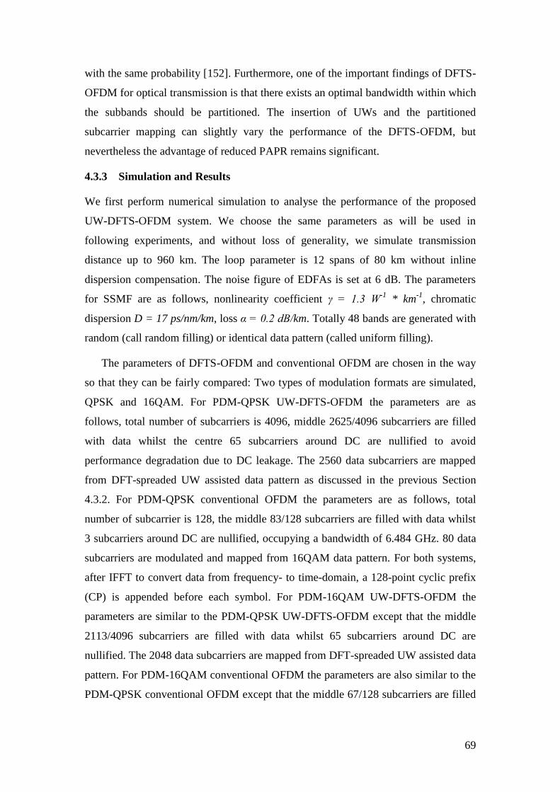
69
with the same probability [152]. Furthermore, one of the important findings of DFTS-
OFDM for optical transmission is that there exists an optimal bandwidth within which
the subbands should be partitioned. The insertion of UWs and the partitioned
subcarrier mapping can slightly vary the performance of the DFTS-OFDM, but
nevertheless the advantage of reduced PAPR remains significant.
4.3.3 Simulation and Results
We first perform numerical simulation to analyse the performance of the proposed
UW-DFTS-OFDM system. We choose the same parameters as will be used in
following experiments, and without loss of generality, we simulate transmission
distance up to 960 km. The loop parameter is 12 spans of 80 km without inline
dispersion compensation. The noise figure of EDFAs is set at 6 dB. The parameters
for SSMF are as follows, nonlinearity coefficient γ = 1.3 W-1
* km-1
, chromatic
dispersion D = 17 ps/nm/km, loss α = 0.2 dB/km. Totally 48 bands are generated with
random (call random filling) or identical data pattern (called uniform filling).
The parameters of DFTS-OFDM and conventional OFDM are chosen in the way
so that they can be fairly compared: Two types of modulation formats are simulated,
QPSK and 16QAM. For PDM-QPSK UW-DFTS-OFDM the parameters are as
follows, total number of subcarriers is 4096, middle 2625/4096 subcarriers are filled
with data whilst the centre 65 subcarriers around DC are nullified to avoid
performance degradation due to DC leakage. The 2560 data subcarriers are mapped
from DFT-spreaded UW assisted data pattern as discussed in the previous Section
4.3.2. For PDM-QPSK conventional OFDM the parameters are as follows, total
number of subcarrier is 128, the middle 83/128 subcarriers are filled with data whilst
3 subcarriers around DC are nullified, occupying a bandwidth of 6.484 GHz. 80 data
subcarriers are modulated and mapped from 16QAM data pattern. For both systems,
after IFFT to convert data from frequency- to time-domain, a 128-point cyclic prefix
(CP) is appended before each symbol. For PDM-16QAM UW-DFTS-OFDM the
parameters are similar to the PDM-QPSK UW-DFTS-OFDM except that the middle
2113/4096 subcarriers are filled with data whilst 65 subcarriers around DC are
nullified. The 2048 data subcarriers are mapped from DFT-spreaded UW assisted data
pattern. For PDM-16QAM conventional OFDM the parameters are also similar to the
PDM-QPSK conventional OFDM except that the middle 67/128 subcarriers are filled
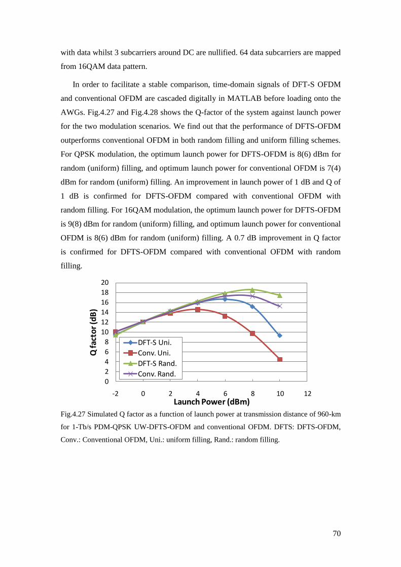
70
with data whilst 3 subcarriers around DC are nullified. 64 data subcarriers are mapped
from 16QAM data pattern.
In order to facilitate a stable comparison, time-domain signals of DFT-S OFDM
and conventional OFDM are cascaded digitally in MATLAB before loading onto the
AWGs. Fig.4.27 and Fig.4.28 shows the Q-factor of the system against launch power
for the two modulation scenarios. We find out that the performance of DFTS-OFDM
outperforms conventional OFDM in both random filling and uniform filling schemes.
For QPSK modulation, the optimum launch power for DFTS-OFDM is 8(6) dBm for
random (uniform) filling, and optimum launch power for conventional OFDM is 7(4)
dBm for random (uniform) filling. An improvement in launch power of 1 dB and Q of
1 dB is confirmed for DFTS-OFDM compared with conventional OFDM with
random filling. For 16QAM modulation, the optimum launch power for DFTS-OFDM
is 9(8) dBm for random (uniform) filling, and optimum launch power for conventional
OFDM is 8(6) dBm for random (uniform) filling. A 0.7 dB improvement in Q factor
is confirmed for DFTS-OFDM compared with conventional OFDM with random
filling.
0
2
4
6
8
10
12
14
16
18
20
-2 0 2 4 6 8 10 12
Q fa
cto
r (d
B)
Launch Power (dBm)
DFT-S Uni.
Conv. Uni.
DFT-S Rand.
Conv. Rand.
Fig.4.27 Simulated Q factor as a function of launch power at transmission distance of 960-km
for 1-Tb/s PDM-QPSK UW-DFTS-OFDM and conventional OFDM. DFTS: DFTS-OFDM,
Conv.: Conventional OFDM, Uni.: uniform filling, Rand.: random filling.
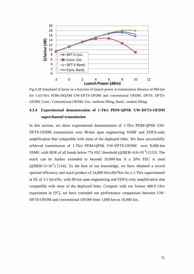
71
0
2
4
6
8
10
12
14
16
18
20
-2 0 2 4 6 8 10 12
Q fa
cto
r (d
B)
Luanch Power (dBm)
DFT-S Uni.
Conv. Uni.
DFT-S Rand.
Conv. Rand.
Fig.4.28 Simulated Q factor as a function of launch power at transmission distance of 960-km
for 1.63-Tb/s PDM-16QAM UW-DFTS-OFDM and conventional OFDM. DFTS: DFTS-
OFDM, Conv.: Conventional OFDM, Uni.: uniform filling, Rand.: random filling.
4.3.4 Experimental demonstration of 1-Tb/s PDM-QPSK UW-DFTS-OFDM
superchannel transmission
In this section, we show experimental demonstration of 1-Tb/s PDM-QPSK UW-
DFTS-OFDM transmission over 80-km span engineering SSMF and EDFA-only
amplification that compatible with most of the deployed links. We have successfully
achieved transmission of 1-Tb/s PDM-QPSK UW-DFTS-OFDM over 8,000-km
SSMF, with BER of all bands below 7% FEC threshold (@BER=4.6×10⁻³
) [153]. The
reach can be further extended to beyond 10,000-km if a 20% FEC is used
(@BER=2×10⁻²
) [154]. To the best of our knowledge, we have obtained a record
spectral efficiency and reach product of 24,800 bit/s/Hz*km for a 1-Tb/s superchannel
at SE of 3.1 bit/s/Hz, with 80-km span engineering and EDFA-only amplification that
compatible with most of the deployed links. Compare with our former 440.8 Gb/s
experiment in [97], we have extended our performance comparison between UW-
DFTS-OFDM and conventional OFDM from 1,000 km to 10,000 km.
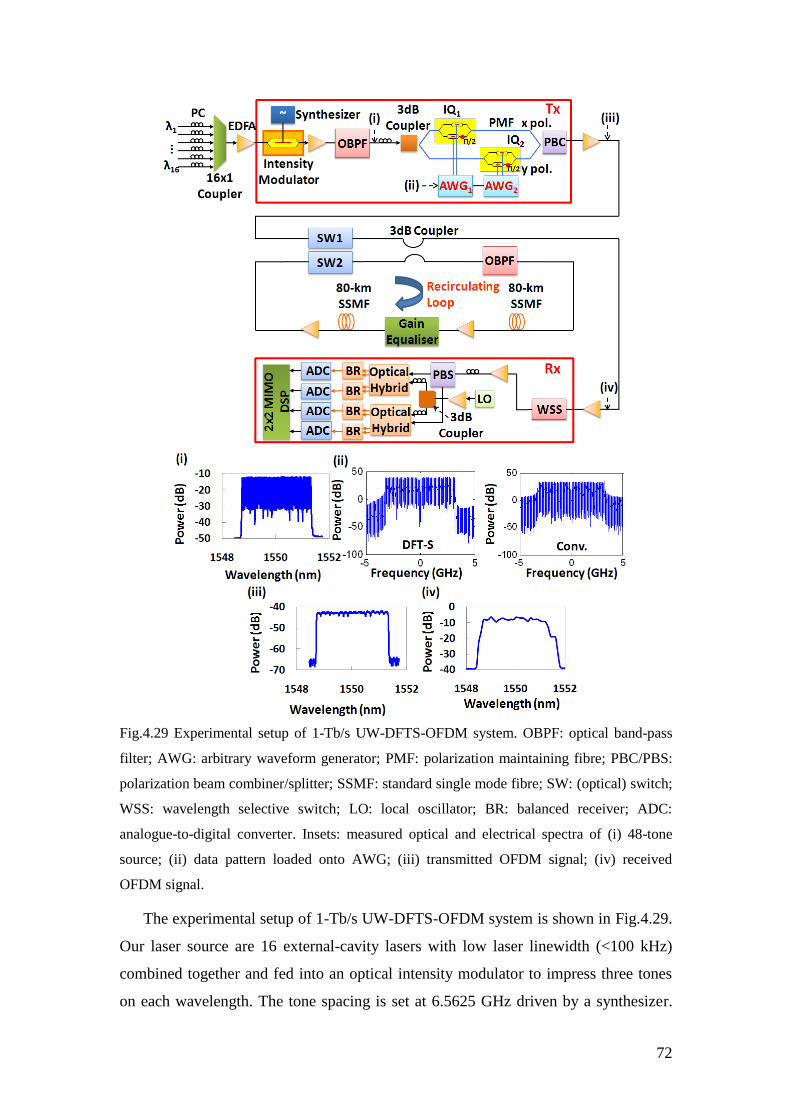
72
Fig.4.29 Experimental setup of 1-Tb/s UW-DFTS-OFDM system. OBPF: optical band-pass
filter; AWG: arbitrary waveform generator; PMF: polarization maintaining fibre; PBC/PBS:
polarization beam combiner/splitter; SSMF: standard single mode fibre; SW: (optical) switch;
WSS: wavelength selective switch; LO: local oscillator; BR: balanced receiver; ADC:
analogue-to-digital converter. Insets: measured optical and electrical spectra of (i) 48-tone
source; (ii) data pattern loaded onto AWG; (iii) transmitted OFDM signal; (iv) received
OFDM signal.
The experimental setup of 1-Tb/s UW-DFTS-OFDM system is shown in Fig.4.29.
Our laser source are 16 external-cavity lasers with low laser linewidth (<100 kHz)
combined together and fed into an optical intensity modulator to impress three tones
on each wavelength. The tone spacing is set at 6.5625 GHz driven by a synthesizer.
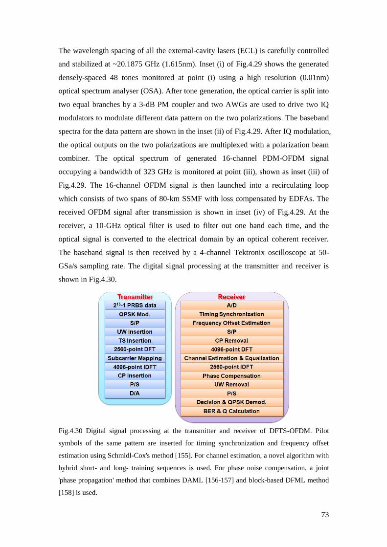
73
The wavelength spacing of all the external-cavity lasers (ECL) is carefully controlled
and stabilized at ~20.1875 GHz (1.615nm). Inset (i) of Fig.4.29 shows the generated
densely-spaced 48 tones monitored at point (i) using a high resolution (0.01nm)
optical spectrum analyser (OSA). After tone generation, the optical carrier is split into
two equal branches by a 3-dB PM coupler and two AWGs are used to drive two IQ
modulators to modulate different data pattern on the two polarizations. The baseband
spectra for the data pattern are shown in the inset (ii) of Fig.4.29. After IQ modulation,
the optical outputs on the two polarizations are multiplexed with a polarization beam
combiner. The optical spectrum of generated 16-channel PDM-OFDM signal
occupying a bandwidth of 323 GHz is monitored at point (iii), shown as inset (iii) of
Fig.4.29. The 16-channel OFDM signal is then launched into a recirculating loop
which consists of two spans of 80-km SSMF with loss compensated by EDFAs. The
received OFDM signal after transmission is shown in inset (iv) of Fig.4.29. At the
receiver, a 10-GHz optical filter is used to filter out one band each time, and the
optical signal is converted to the electrical domain by an optical coherent receiver.
The baseband signal is then received by a 4-channel Tektronix oscilloscope at 50-
GSa/s sampling rate. The digital signal processing at the transmitter and receiver is
shown in Fig.4.30.
Fig.4.30 Digital signal processing at the transmitter and receiver of DFTS-OFDM. Pilot
symbols of the same pattern are inserted for timing synchronization and frequency offset
estimation using Schmidl-Cox's method [155]. For channel estimation, a novel algorithm with
hybrid short- and long- training sequences is used. For phase noise compensation, a joint
'phase propagation' method that combines DAML [156-157] and block-based DFML method
[158] is used.
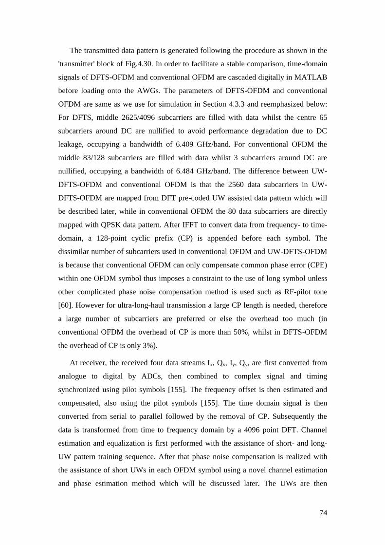
74
The transmitted data pattern is generated following the procedure as shown in the
'transmitter' block of Fig.4.30. In order to facilitate a stable comparison, time-domain
signals of DFTS-OFDM and conventional OFDM are cascaded digitally in MATLAB
before loading onto the AWGs. The parameters of DFTS-OFDM and conventional
OFDM are same as we use for simulation in Section 4.3.3 and reemphasized below:
For DFTS, middle 2625/4096 subcarriers are filled with data whilst the centre 65
subcarriers around DC are nullified to avoid performance degradation due to DC
leakage, occupying a bandwidth of 6.409 GHz/band. For conventional OFDM the
middle 83/128 subcarriers are filled with data whilst 3 subcarriers around DC are
nullified, occupying a bandwidth of 6.484 GHz/band. The difference between UW-
DFTS-OFDM and conventional OFDM is that the 2560 data subcarriers in UW-
DFTS-OFDM are mapped from DFT pre-coded UW assisted data pattern which will
be described later, while in conventional OFDM the 80 data subcarriers are directly
mapped with QPSK data pattern. After IFFT to convert data from frequency- to time-
domain, a 128-point cyclic prefix (CP) is appended before each symbol. The
dissimilar number of subcarriers used in conventional OFDM and UW-DFTS-OFDM
is because that conventional OFDM can only compensate common phase error (CPE)
within one OFDM symbol thus imposes a constraint to the use of long symbol unless
other complicated phase noise compensation method is used such as RF-pilot tone
[60]. However for ultra-long-haul transmission a large CP length is needed, therefore
a large number of subcarriers are preferred or else the overhead too much (in
conventional OFDM the overhead of CP is more than 50%, whilst in DFTS-OFDM
the overhead of CP is only 3%).
At receiver, the received four data streams Ix, Qx, Iy, Qy, are first converted from
analogue to digital by ADCs, then combined to complex signal and timing
synchronized using pilot symbols [155]. The frequency offset is then estimated and
compensated, also using the pilot symbols [155]. The time domain signal is then
converted from serial to parallel followed by the removal of CP. Subsequently the
data is transformed from time to frequency domain by a 4096 point DFT. Channel
estimation and equalization is first performed with the assistance of short- and long-
UW pattern training sequence. After that phase noise compensation is realized with
the assistance of short UWs in each OFDM symbol using a novel channel estimation
and phase estimation method which will be discussed later. The UWs are then
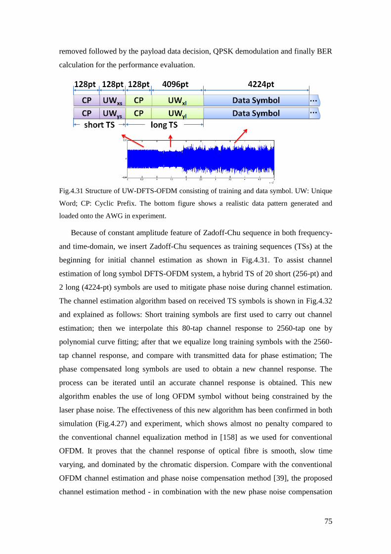
75
removed followed by the payload data decision, QPSK demodulation and finally BER
calculation for the performance evaluation.
Fig.4.31 Structure of UW-DFTS-OFDM consisting of training and data symbol. UW: Unique
Word; CP: Cyclic Prefix. The bottom figure shows a realistic data pattern generated and
loaded onto the AWG in experiment.
Because of constant amplitude feature of Zadoff-Chu sequence in both frequency-
and time-domain, we insert Zadoff-Chu sequences as training sequences (TSs) at the
beginning for initial channel estimation as shown in Fig.4.31. To assist channel
estimation of long symbol DFTS-OFDM system, a hybrid TS of 20 short (256-pt) and
2 long (4224-pt) symbols are used to mitigate phase noise during channel estimation.
The channel estimation algorithm based on received TS symbols is shown in Fig.4.32
and explained as follows: Short training symbols are first used to carry out channel
estimation; then we interpolate this 80-tap channel response to 2560-tap one by
polynomial curve fitting; after that we equalize long training symbols with the 2560-
tap channel response, and compare with transmitted data for phase estimation; The
phase compensated long symbols are used to obtain a new channel response. The
process can be iterated until an accurate channel response is obtained. This new
algorithm enables the use of long OFDM symbol without being constrained by the
laser phase noise. The effectiveness of this new algorithm has been confirmed in both
simulation (Fig.4.27) and experiment, which shows almost no penalty compared to
the conventional channel equalization method in [158] as we used for conventional
OFDM. It proves that the channel response of optical fibre is smooth, slow time
varying, and dominated by the chromatic dispersion. Compare with the conventional
OFDM channel estimation and phase noise compensation method [39], the proposed
channel estimation method - in combination with the new phase noise compensation
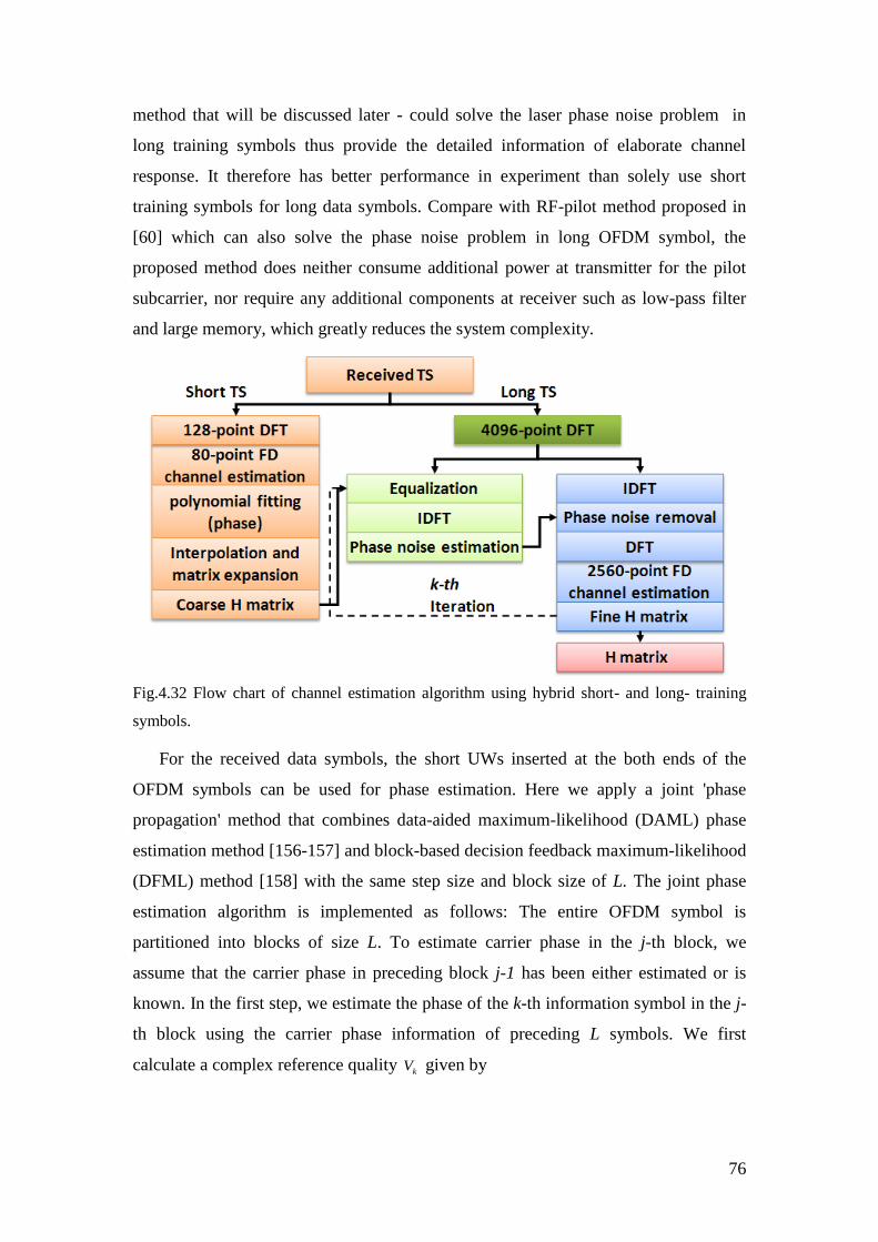
76
method that will be discussed later - could solve the laser phase noise problem in
long training symbols thus provide the detailed information of elaborate channel
response. It therefore has better performance in experiment than solely use short
training symbols for long data symbols. Compare with RF-pilot method proposed in
[60] which can also solve the phase noise problem in long OFDM symbol, the
proposed method does neither consume additional power at transmitter for the pilot
subcarrier, nor require any additional components at receiver such as low-pass filter
and large memory, which greatly reduces the system complexity.
Fig.4.32 Flow chart of channel estimation algorithm using hybrid short- and long- training
symbols.
For the received data symbols, the short UWs inserted at the both ends of the
OFDM symbols can be used for phase estimation. Here we apply a joint 'phase
propagation' method that combines data-aided maximum-likelihood (DAML) phase
estimation method [156-157] and block-based decision feedback maximum-likelihood
(DFML) method [158] with the same step size and block size of L. The joint phase
estimation algorithm is implemented as follows: The entire OFDM symbol is
partitioned into blocks of size L. To estimate carrier phase in the j-th block, we
assume that the carrier phase in preceding block j-1 has been either estimated or is
known. In the first step, we estimate the phase of the k-th information symbol in the j-
th block using the carrier phase information of preceding L symbols. We first
calculate a complex reference quality kV given by
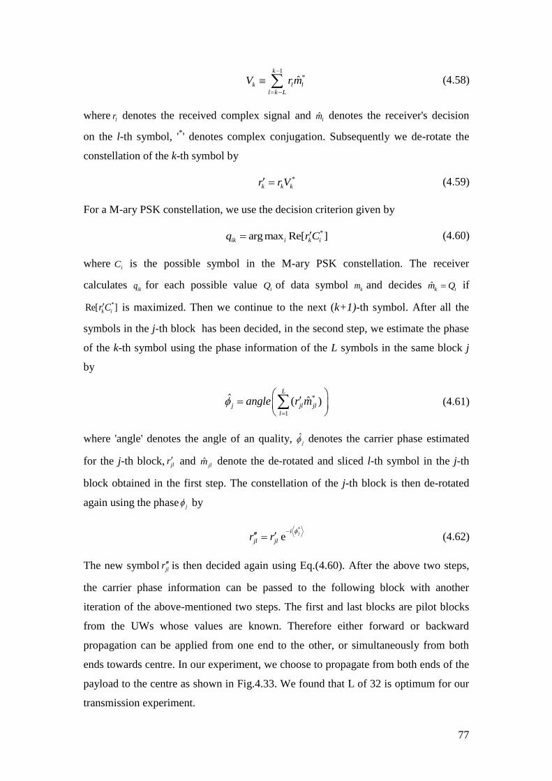
77
1
*ˆk
k l l
l k L
V r m
(4.58)
wherelr denotes the received complex signal and ˆ
lm denotes the receiver's decision
on the l-th symbol, '*' denotes complex conjugation. Subsequently we de-rotate the
constellation of the k-th symbol by
*
k k kr r V (4.59)
For a M-ary PSK constellation, we use the decision criterion given by
*arg max Re[ ]ik i k iq r C (4.60)
whereiC is the possible symbol in the M-ary PSK constellation. The receiver
calculates ikq for each possible value
iQ of data symbol km and decides ˆ
k im Q if
*Re[ ]k ir C is maximized. Then we continue to the next (k+1)-th symbol. After all the
symbols in the j-th block has been decided, in the second step, we estimate the phase
of the k-th symbol using the phase information of the L symbols in the same block j
by
*
1
ˆ ˆ( )L
j jl jl
l
angle r m
(4.61)
where 'angle' denotes the angle of an quality, ˆj denotes the carrier phase estimated
for the j-th block, jlr and ˆjlm denote the de-rotated and sliced l-th symbol in the j-th
block obtained in the first step. The constellation of the j-th block is then de-rotated
again using the phase j by
*
eji
jl jlr r
(4.62)
The new symbol jlr is then decided again using Eq.(4.60). After the above two steps,
the carrier phase information can be passed to the following block with another
iteration of the above-mentioned two steps. The first and last blocks are pilot blocks
from the UWs whose values are known. Therefore either forward or backward
propagation can be applied from one end to the other, or simultaneously from both
ends towards centre. In our experiment, we choose to propagate from both ends of the
payload to the centre as shown in Fig.4.33. We found that L of 32 is optimum for our
transmission experiment.
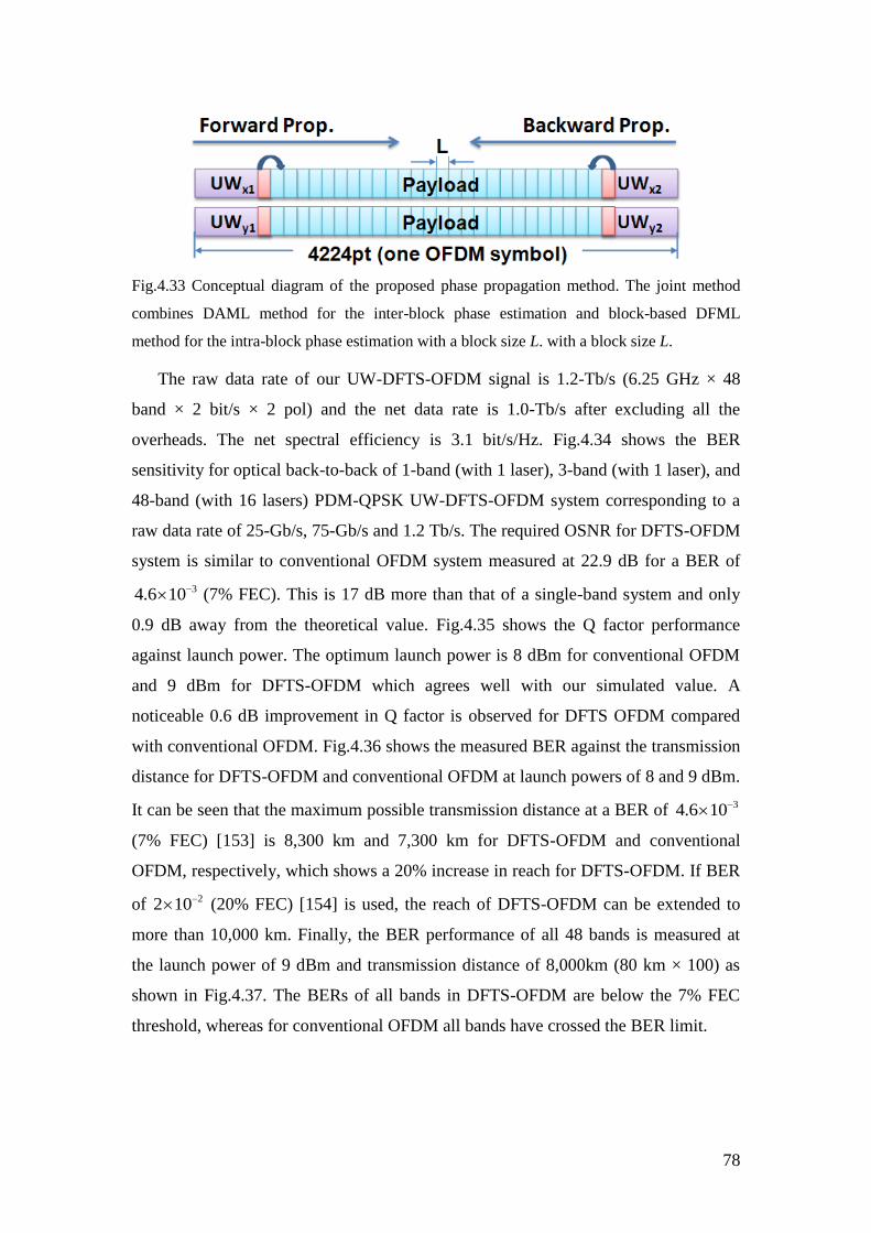
78
Fig.4.33 Conceptual diagram of the proposed phase propagation method. The joint method
combines DAML method for the inter-block phase estimation and block-based DFML
method for the intra-block phase estimation with a block size L. with a block size L.
The raw data rate of our UW-DFTS-OFDM signal is 1.2-Tb/s (6.25 GHz × 48
band × 2 bit/s × 2 pol) and the net data rate is 1.0-Tb/s after excluding all the
overheads. The net spectral efficiency is 3.1 bit/s/Hz. Fig.4.34 shows the BER
sensitivity for optical back-to-back of 1-band (with 1 laser), 3-band (with 1 laser), and
48-band (with 16 lasers) PDM-QPSK UW-DFTS-OFDM system corresponding to a
raw data rate of 25-Gb/s, 75-Gb/s and 1.2 Tb/s. The required OSNR for DFTS-OFDM
system is similar to conventional OFDM system measured at 22.9 dB for a BER of
34.6 10 (7% FEC). This is 17 dB more than that of a single-band system and only
0.9 dB away from the theoretical value. Fig.4.35 shows the Q factor performance
against launch power. The optimum launch power is 8 dBm for conventional OFDM
and 9 dBm for DFTS-OFDM which agrees well with our simulated value. A
noticeable 0.6 dB improvement in Q factor is observed for DFTS OFDM compared
with conventional OFDM. Fig.4.36 shows the measured BER against the transmission
distance for DFTS-OFDM and conventional OFDM at launch powers of 8 and 9 dBm.
It can be seen that the maximum possible transmission distance at a BER of 34.6 10
(7% FEC) [153] is 8,300 km and 7,300 km for DFTS-OFDM and conventional
OFDM, respectively, which shows a 20% increase in reach for DFTS-OFDM. If BER
of 22 10 (20% FEC) [154] is used, the reach of DFTS-OFDM can be extended to
more than 10,000 km. Finally, the BER performance of all 48 bands is measured at
the launch power of 9 dBm and transmission distance of 8,000km (80 km × 100) as
shown in Fig.4.37. The BERs of all bands in DFTS-OFDM are below the 7% FEC
threshold, whereas for conventional OFDM all bands have crossed the BER limit.
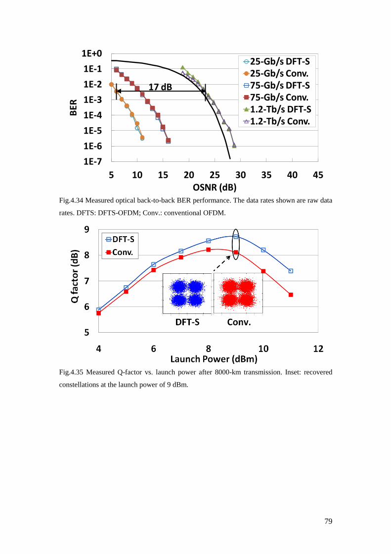
79
1E-7
1E-6
1E-5
1E-4
1E-3
1E-2
1E-1
1E+0
5 10 15 20 25 30 35 40 45
BER
OSNR (dB)
25-Gb/s DFT-S25-Gb/s Conv.75-Gb/s DFT-S75-Gb/s Conv.1.2-Tb/s DFT-S1.2-Tb/s Conv.
17 dB
Fig.4.34 Measured optical back-to-back BER performance. The data rates shown are raw data
rates. DFTS: DFTS-OFDM; Conv.: conventional OFDM.
Fig.4.35 Measured Q-factor vs. launch power after 8000-km transmission. Inset: recovered
constellations at the launch power of 9 dBm.
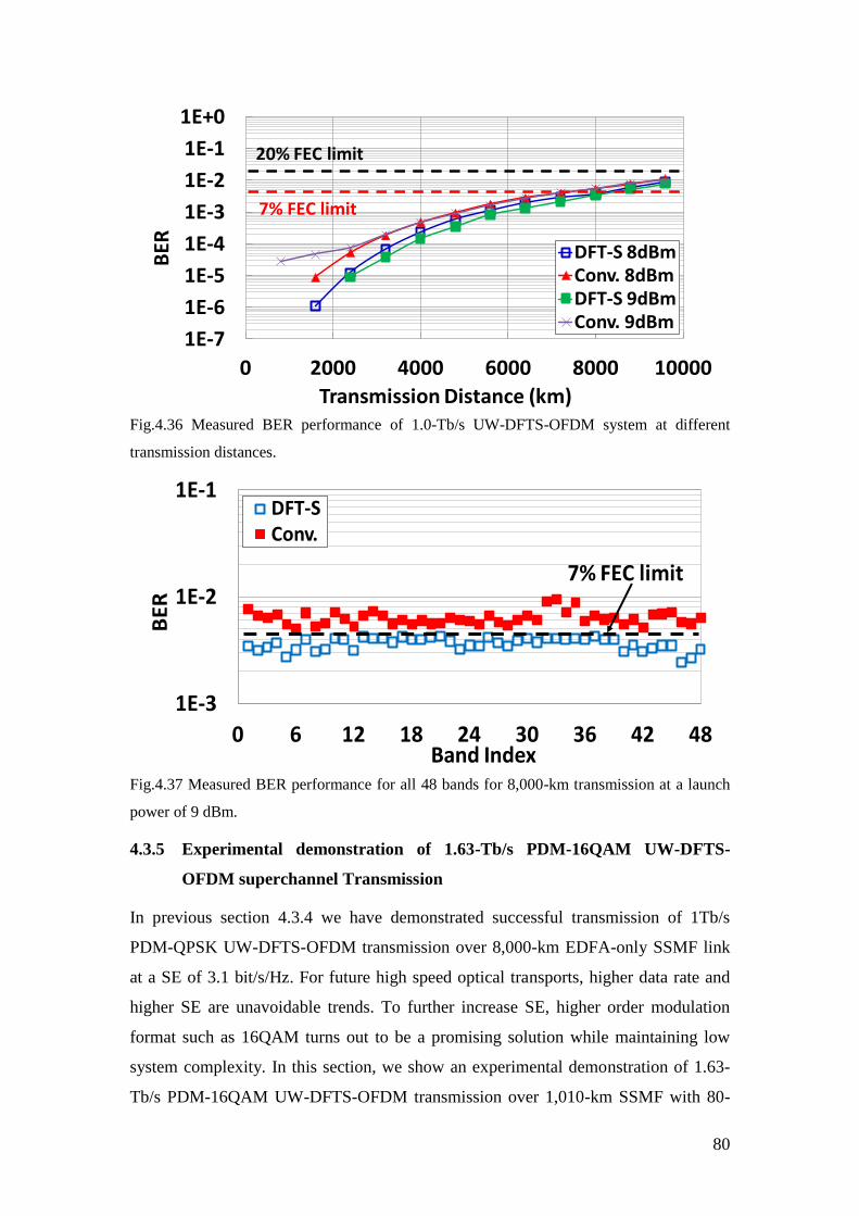
80
1E-7
1E-6
1E-5
1E-4
1E-3
1E-2
1E-1
1E+0
0 2000 4000 6000 8000 10000
BER
Transmission Distance (km)
DFT-S 8dBmConv. 8dBmDFT-S 9dBmConv. 9dBm
7% FEC limit
20% FEC limit
Fig.4.36 Measured BER performance of 1.0-Tb/s UW-DFTS-OFDM system at different
transmission distances.
1E-3
1E-2
1E-1
0 6 12 18 24 30 36 42 48
BE
R
Band Index
DFT-SConv.
7% FEC limit
Fig.4.37 Measured BER performance for all 48 bands for 8,000-km transmission at a launch
power of 9 dBm.
4.3.5 Experimental demonstration of 1.63-Tb/s PDM-16QAM UW-DFTS-
OFDM superchannel Transmission
In previous section 4.3.4 we have demonstrated successful transmission of 1Tb/s
PDM-QPSK UW-DFTS-OFDM transmission over 8,000-km EDFA-only SSMF link
at a SE of 3.1 bit/s/Hz. For future high speed optical transports, higher data rate and
higher SE are unavoidable trends. To further increase SE, higher order modulation
format such as 16QAM turns out to be a promising solution while maintaining low
system complexity. In this section, we show an experimental demonstration of 1.63-
Tb/s PDM-16QAM UW-DFTS-OFDM transmission over 1,010-km SSMF with 80-
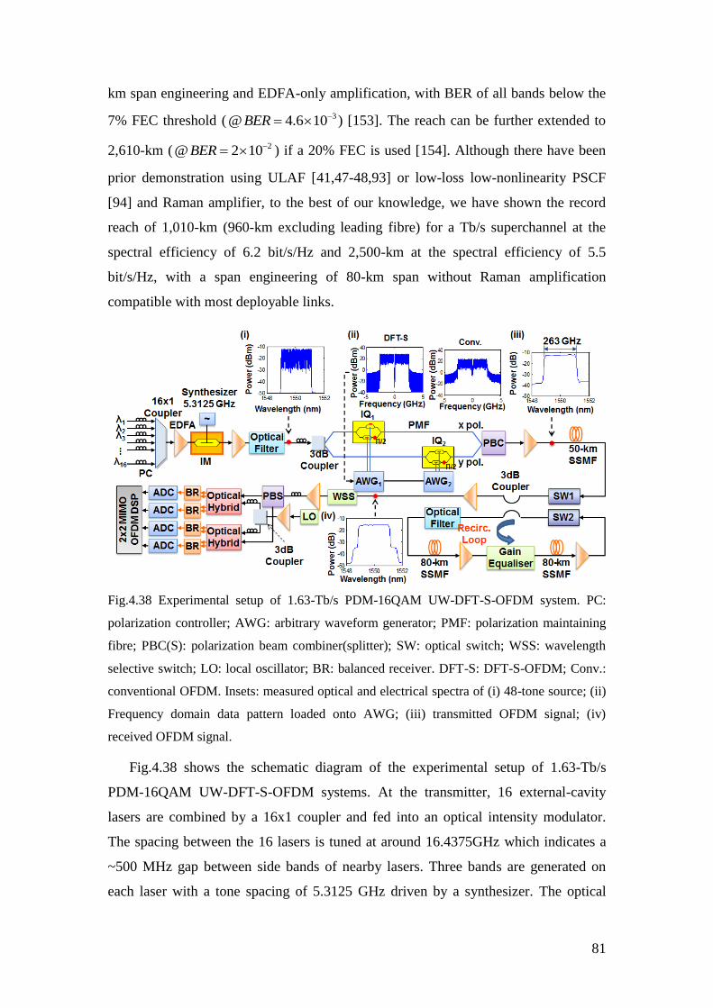
81
km span engineering and EDFA-only amplification, with BER of all bands below the
7% FEC threshold ( 3@ 4.6 10BER ) [153]. The reach can be further extended to
2,610-km ( 2@ 2 10BER ) if a 20% FEC is used [154]. Although there have been
prior demonstration using ULAF [41,47-48,93] or low-loss low-nonlinearity PSCF
[94] and Raman amplifier, to the best of our knowledge, we have shown the record
reach of 1,010-km (960-km excluding leading fibre) for a Tb/s superchannel at the
spectral efficiency of 6.2 bit/s/Hz and 2,500-km at the spectral efficiency of 5.5
bit/s/Hz, with a span engineering of 80-km span without Raman amplification
compatible with most deployable links.
Fig.4.38 Experimental setup of 1.63-Tb/s PDM-16QAM UW-DFT-S-OFDM system. PC:
polarization controller; AWG: arbitrary waveform generator; PMF: polarization maintaining
fibre; PBC(S): polarization beam combiner(splitter); SW: optical switch; WSS: wavelength
selective switch; LO: local oscillator; BR: balanced receiver. DFT-S: DFT-S-OFDM; Conv.:
conventional OFDM. Insets: measured optical and electrical spectra of (i) 48-tone source; (ii)
Frequency domain data pattern loaded onto AWG; (iii) transmitted OFDM signal; (iv)
received OFDM signal.
Fig.4.38 shows the schematic diagram of the experimental setup of 1.63-Tb/s
PDM-16QAM UW-DFT-S-OFDM systems. At the transmitter, 16 external-cavity
lasers are combined by a 16x1 coupler and fed into an optical intensity modulator.
The spacing between the 16 lasers is tuned at around 16.4375GHz which indicates a
~500 MHz gap between side bands of nearby lasers. Three bands are generated on
each laser with a tone spacing of 5.3125 GHz driven by a synthesizer. The optical
82
spectrum of generated densely-spaced 48 bands is monitored by a high-resolution
OSA shown as the inset (i) of Fig.4.38. After tone generation, the optical carrier is
split into two equal branches. Two synchronized AWGs are used to drive two IQ
modulators with independent data patterns, which enable the UWs in both TS and
data.
The parameters of DFTS OFDM and conventional OFDM are same as used for
simulation in Section 4.3.3 and reemphasized as below: total number of subcarriers is
4096, out of which the middle 2113/4096 subcarriers are filled with data whilst 65
subcarriers around DC are nullified to avoid degradation due to DC leakage,
occupying a bandwidth of 5.159 GHz/band. The 2048 data subcarriers are mapped
from DFT-spreaded UW assisted data pattern. Similar as we did in PDM-QPSK UW-
DFTS-OFDM, a hybrid training sequence of 20 short (144-pt) and 2 long (4112-pt)
symbols is also used to mitigate phase noise during channel estimation. For
conventional OFDM, total number of subcarrier is 128, out of which the middle
67/128 subcarriers are filled with data whilst 3 subcarriers around DC are nullified,
occupying a bandwidth of 5.234GHz/band. The 64 data subcarriers are also
modulated and mapped with 16QAM data pattern. In order to facilitate a stable
comparison, time-domain signals of DFT-S OFDM and conventional OFDM are
cascaded digitally in MATLAB before loading onto the AWGs. The baseband spectra
for the data pattern are shown in the inset (ii) of Fig.4.38.
After IQ modulation, the optical outputs on the two polarizations are multiplexed
by a polarization beam combiner. The optical spectrum of a 16-channel PDM-OFDM
signal occupying a bandwidth of 263 GHz is monitored and shown as inset (iii) of
Fig.4.38. The 16-channel OFDM signal first passes through a 50-km SSMF fibre with
low optical power (2 dBm) to de-correlate the signals in all bands, and is then
launched into a recirculation loop which consists of two spans of 80-km SSMF loss-
compensated by EDFAs. At the receiver, a 10-GHz optical filter is used to filter out
one band each time, and the optical signal is converted to the electrical domain by an
optical coherent receiver. The baseband signal is then received by a 4-channel
Tektronix oscilloscope at 50GSa/s sampling rate. The timing synchronization and
frequency offset is done using UWs. After serial-to-parallel conversion and CP
removal, the time-domain signal is transformed into the frequency domain using a
4096-pt DFT. With the knowledge of estimated channel matrix H, the data symbol
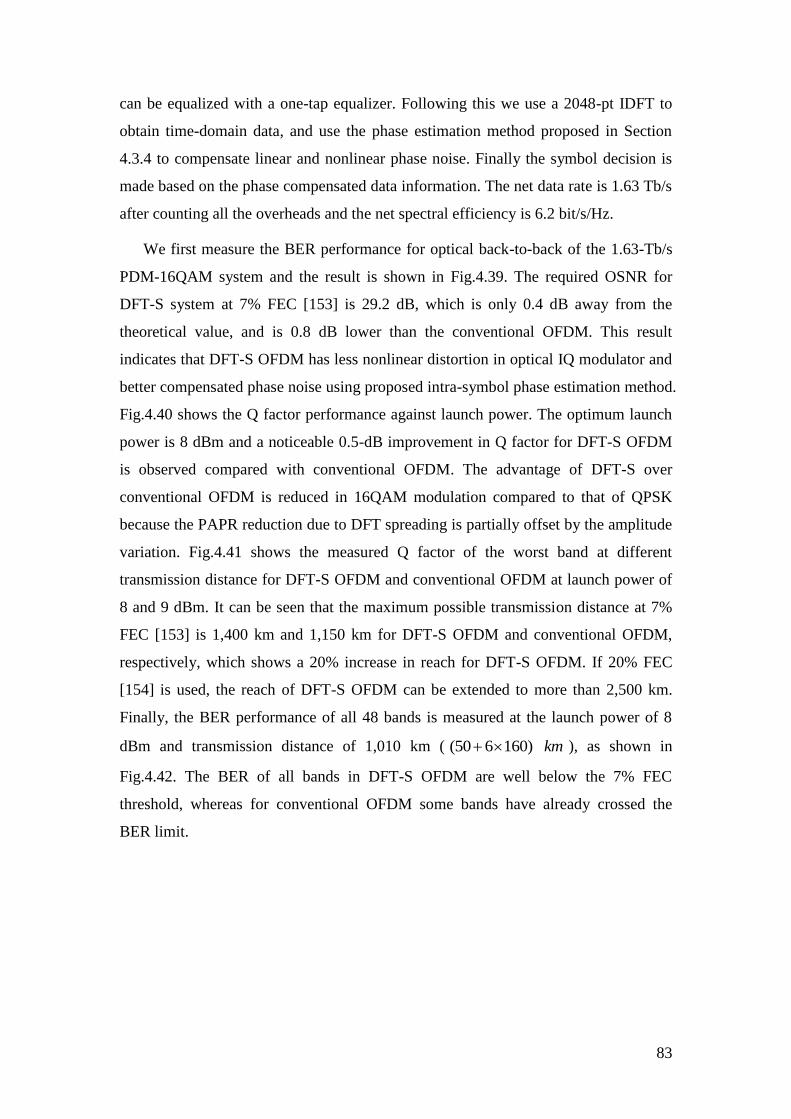
83
can be equalized with a one-tap equalizer. Following this we use a 2048-pt IDFT to
obtain time-domain data, and use the phase estimation method proposed in Section
4.3.4 to compensate linear and nonlinear phase noise. Finally the symbol decision is
made based on the phase compensated data information. The net data rate is 1.63 Tb/s
after counting all the overheads and the net spectral efficiency is 6.2 bit/s/Hz.
We first measure the BER performance for optical back-to-back of the 1.63-Tb/s
PDM-16QAM system and the result is shown in Fig.4.39. The required OSNR for
DFT-S system at 7% FEC [153] is 29.2 dB, which is only 0.4 dB away from the
theoretical value, and is 0.8 dB lower than the conventional OFDM. This result
indicates that DFT-S OFDM has less nonlinear distortion in optical IQ modulator and
better compensated phase noise using proposed intra-symbol phase estimation method.
Fig.4.40 shows the Q factor performance against launch power. The optimum launch
power is 8 dBm and a noticeable 0.5-dB improvement in Q factor for DFT-S OFDM
is observed compared with conventional OFDM. The advantage of DFT-S over
conventional OFDM is reduced in 16QAM modulation compared to that of QPSK
because the PAPR reduction due to DFT spreading is partially offset by the amplitude
variation. Fig.4.41 shows the measured Q factor of the worst band at different
transmission distance for DFT-S OFDM and conventional OFDM at launch power of
8 and 9 dBm. It can be seen that the maximum possible transmission distance at 7%
FEC [153] is 1,400 km and 1,150 km for DFT-S OFDM and conventional OFDM,
respectively, which shows a 20% increase in reach for DFT-S OFDM. If 20% FEC
[154] is used, the reach of DFT-S OFDM can be extended to more than 2,500 km.
Finally, the BER performance of all 48 bands is measured at the launch power of 8
dBm and transmission distance of 1,010 km ( (50 6 160) km ), as shown in
Fig.4.42. The BER of all bands in DFT-S OFDM are well below the 7% FEC
threshold, whereas for conventional OFDM some bands have already crossed the
BER limit.
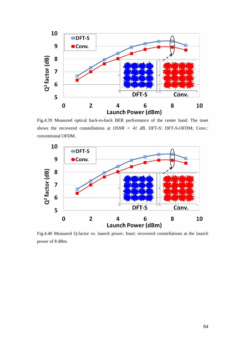
84
Fig.4.39 Measured optical back-to-back BER performance of the center band. The inset
shows the recovered constellations at OSNR = 41 dB. DFT-S: DFT-S-OFDM; Conv.:
conventional OFDM.
Fig.4.40 Measured Q-factor vs. launch power. Inset: recovered constellations at the launch
power of 8 dBm.
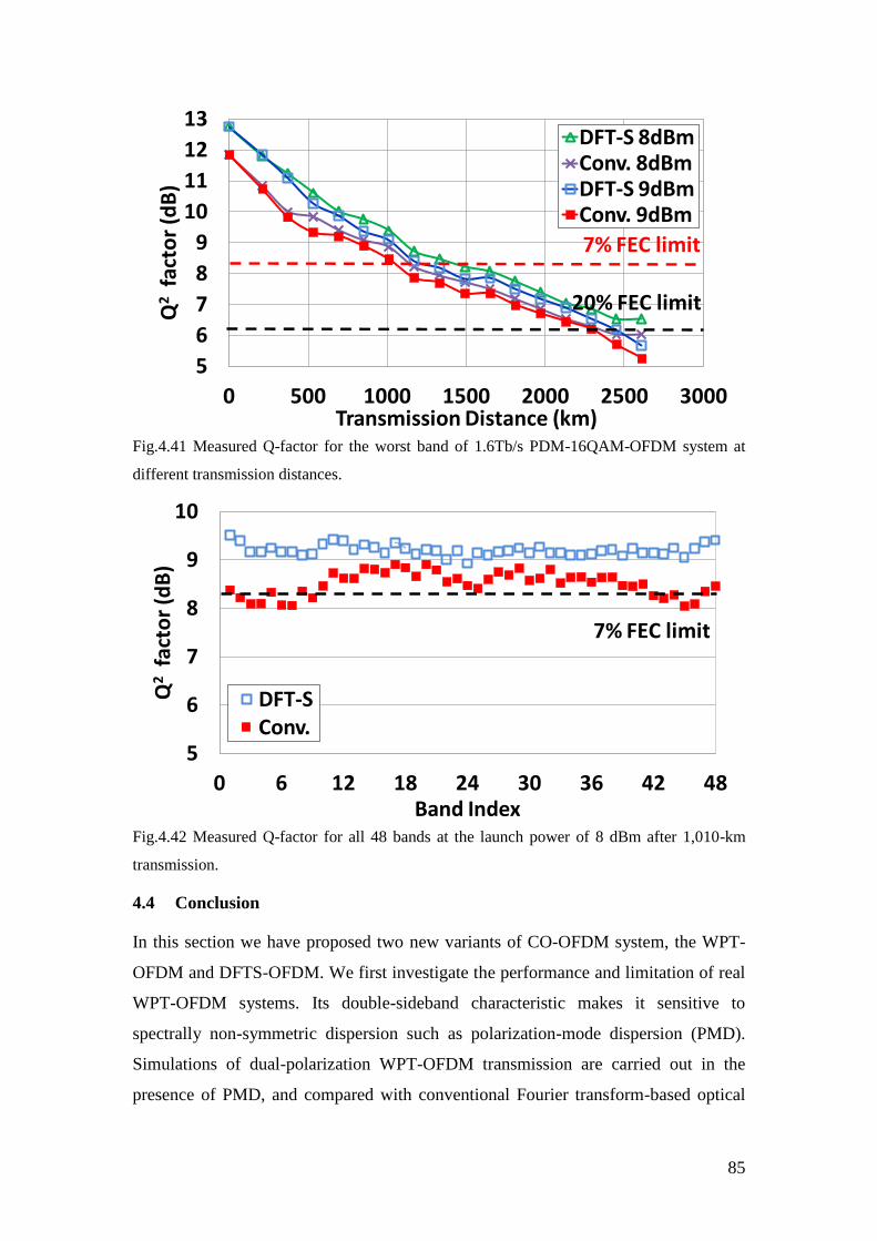
85
5
6
7
8
9
10
11
12
13
0 500 1000 1500 2000 2500 3000
Q2
fact
or
(dB
)
Transmission Distance (km)
DFT-S 8dBmConv. 8dBmDFT-S 9dBmConv. 9dBm
20% FEC limit
7% FEC limit
Fig.4.41 Measured Q-factor for the worst band of 1.6Tb/s PDM-16QAM-OFDM system at
different transmission distances.
5
6
7
8
9
10
0 6 12 18 24 30 36 42 48
Q2
fact
or
(dB
)
Band Index
DFT-SConv.
7% FEC limit
Fig.4.42 Measured Q-factor for all 48 bands at the launch power of 8 dBm after 1,010-km
transmission.
4.4 Conclusion
In this section we have proposed two new variants of CO-OFDM system, the WPT-
OFDM and DFTS-OFDM. We first investigate the performance and limitation of real
WPT-OFDM systems. Its double-sideband characteristic makes it sensitive to
spectrally non-symmetric dispersion such as polarization-mode dispersion (PMD).
Simulations of dual-polarization WPT-OFDM transmission are carried out in the
presence of PMD, and compared with conventional Fourier transform-based optical
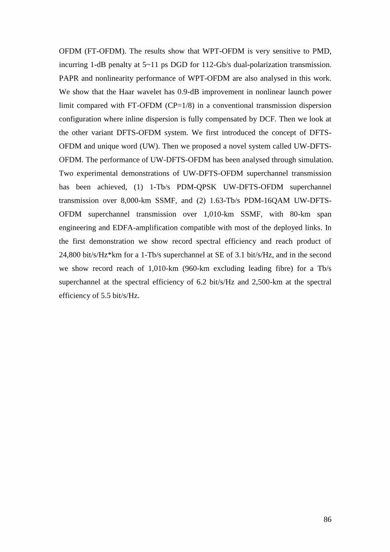
86
OFDM (FT-OFDM). The results show that WPT-OFDM is very sensitive to PMD,
incurring 1-dB penalty at 5~11 ps DGD for 112-Gb/s dual-polarization transmission.
PAPR and nonlinearity performance of WPT-OFDM are also analysed in this work.
We show that the Haar wavelet has 0.9-dB improvement in nonlinear launch power
limit compared with FT-OFDM (CP=1/8) in a conventional transmission dispersion
configuration where inline dispersion is fully compensated by DCF. Then we look at
the other variant DFTS-OFDM system. We first introduced the concept of DFTS-
OFDM and unique word (UW). Then we proposed a novel system called UW-DFTS-
OFDM. The performance of UW-DFTS-OFDM has been analysed through simulation.
Two experimental demonstrations of UW-DFTS-OFDM superchannel transmission
has been achieved, (1) 1-Tb/s PDM-QPSK UW-DFTS-OFDM superchannel
transmission over 8,000-km SSMF, and (2) 1.63-Tb/s PDM-16QAM UW-DFTS-
OFDM superchannel transmission over 1,010-km SSMF, with 80-km span
engineering and EDFA-amplification compatible with most of the deployed links. In
the first demonstration we show record spectral efficiency and reach product of
24,800 bit/s/Hz*km for a 1-Tb/s superchannel at SE of 3.1 bit/s/Hz, and in the second
we show record reach of 1,010-km (960-km excluding leading fibre) for a Tb/s
superchannel at the spectral efficiency of 6.2 bit/s/Hz and 2,500-km at the spectral
efficiency of 5.5 bit/s/Hz.
87
5 Few-Mode and Two-Mode Fibre
The highest reported single optical fibre data transmission speed has reached over
100-Tb/s [14-15]. However, there is a need to continue enhancing the total data
transmission capacity while keeping the signals within the available optical spectrum
of the conventional Erbium doped fibre amplifier (EDFA), which translates into the
requirement for increased spectral efficiency (SE, expressed in b/s/Hz). Although
Shannon's theory predicts SE to increase with higher received SNR as a result of
increased transmission power, fibre nonlinearity imposes a hard constraint on the
channel capacity [24]. It is foreseen that the saturation of the fibre capacity for on the
SSMFs that we use today is fast coming. Information theory reveals that by adding
another degree of freedom, namely the spatial mode, the fibre capacity of MMF or
FMF can be increased. Therefore it is of great interest to know whether the few-mode
fibre (FMF) such as two-mode fibre (TMF) can offer capacity beyond that of SSMF
in a cost effective manner. In this chapter, we show the design of a practical TMF. We
first review fundamentals of optical fibre and fibre modes. Then we discuss the
parameters and process to fabricate a practical FMF for future space division
multiplexing (SDM) based high speed optical networks. At last we show
characterization of our custom-designed TMF.
5.1 Overview of optical fibres
As was elucidated in Section 1.1.1, an optical fibre normally consists of a core
surrounded by a cladding layer whose refractive index n2 is slightly lower than the
core index n1. If the refractive index of the core n1 is uniform in the core region, it is
called step-index fibre. In contrast, if the refractive index of the core n1 decreases
gradually from centre to core boundary [159-161] it is called a graded-index fibre.
There are two important parameters that characterize an optical fibre: the relative
core-cladding index difference
1 2
1
n n
n
(5.1)
and the normalized frequency (also called V-number) parameter defined as
2 2
0 1 1V k a n n (5.2)
88
where 0 2 /k is the wavenumber, is the wavelength of light, and a is the
radius of core The V number determines how many modes can be supported by the
fibre. The fibre modes denoted here refer to transverse modes and will be discussed in
Section 5.2. It is shown that a step-index fibre supports a single mode if V < 2.405 [76,
-163], which is also called the single mode condition. Optical fibres that support a
single mode are called single-mode fibres (SMF), and can be easily fabricated by
satisfying the single mode condition. On the contrary, optical fibres that support many
modes are called multimode fibres (MMF). The main difference between SMF and
MMF is the core size. The core diameter is typically < 10 μm for SMF, e.g., Corning®
SMF28e®
fibre [164] (a typical SMF and ITU-T G.652.D [165] compliant) the core
diameter is 8.2 μm. For MMF, The recommended core diameter is typically 50 or
62.5 μm, e.g., Corning® ClearCurve
® fibre (a typical MMF and ITU-T G.651.1 [166]
compliant) the core diameter is 50 μm, and Corning® InfiniCor
® fibre has a core
diameter of 62.5 μm. The value of the cladding radius b is less critical as long as it is
large enough to confine the fibre modes, however, a standard value of 62.5b m is
recommended for both SMF and MMF in standards ITU-T G.651 and G.652.
Although there are other types of fibre such as plastic optical fibre which uses
plastic, the commonly used low-loss telecommunication fibre is silica fibre whose
basic material (substrate) is pure silica glass synthesized by fused silica (SiO2). The
core and cladding can be doped during the fabrication process to achieve higher or
lower refractive index than fused silica (≈ 1.44402@1550 nm). Dopants such as GeO2
and P2O5 can increase the refractive index of fused silica, therefore very suitable for
core, whilst dopants such as boron and fluorine can decrease the refractive index of
fused silica, therefore very suitable for cladding. The widely used core-cladding fibre
type can be divided into three categories, (1) doped core with undoped cladding, (2)
undoped core with doped cladding, and (3) doped core with doped cladding. The first
two types are predominant in modern fibre-optic communications, e.g., commercial
available Corning® SMF28e
® fibre has a GeO2 doped core with pure silica cladding.
The second type is usually referred as pure-silica core fibre (PSCF) [94, 167-169],
which has a pure-silica core and fluorine doped cladding. Other dopants are also used
for specific applications, e.g., in fibre amplifiers and lasers the core is codoped with
rare-earth ions such as ErCl3 and Nd2O3.
89
There are typically two stages for the fabrication of optical fibres [170]. The first
stage is to make a cylindrical fibre preform, normally using a vapour-deposition
method such as vapour axial deposition (VAD), outside vapour deposition (OVD),
advanced plasma vapour deposition (APVD),modified chemical vapour deposition
(MCVD), furnace chemical vapour deposition (FCVD) and plasma activated chemical
vapour deposition (PCVD). The latter three methods are very similar. A typical
preform is 1-m long with 2-cm diameter. The second stage is to draw the preform into
a fibre using a precision-feed mechanism and fed into a furnace. The ratio of core-
cladding dimension is preserved during the drawing process. Sophisticated technology
is involved in both stages to guarantee the uniformity of the core size, index profile,
core-clad concentricity, and cladding circularity [170-172].
5.2 Fundamentals of fibre modes
In an optical fibre, the supported fibre modes can be divided into two categories -
guided and unguided modes. Optical fibre can support finite number of guided modes
which are well-confined in the core with low loss. For guided modes, the spatial
distribution ( , )E r must be a solution of the wave equation [162]
2
2 2
20n
c
E E (5.3)
where is the frequency. E is the Fourier transform of the electric field E , i.e.,
1
( , ) ( , )exp( )2
r t r i t d
E E (5.4)
Also they must satisfy appropriate boundary conditions. Optical fibre can also support
a continuum of unguided radiation modes, which usually lead to power leakage (high
loss). Consider the cylindrical symmetry of fibres, Eq. (5.3) can be rewritten with
cylindrical coordinates , and z as
2 2 2
2 2
02 2 2 2
1 10n k
z
E E E EE (5.5)
where 0
2k
c
is the wavenumber. The wave equation for ( , )r E can be written
in a general form as
( , ) ( ) ( )exp( )exp( )z r A F im i z E (5.6)
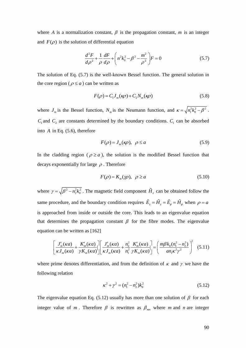
90
where A is a normalization constant, is the propagation constant, m is an integer
and ( )F is the solution of differential equation
2 2
2 2 2
02 2
10
d F dF mn k F
d d
(5.7)
The solution of Eq. (5.7) is the well-known Bessel function. The general solution in
the core region ( a ) can be written as
1 2( ) ( ) ( )m mF C J C N (5.8)
where mJ is the Bessel function, mN is the Neumann function, and 2 2 2
1 0n k .
1C and 2C are constants determined by the boundary conditions. 1C can be absorbed
into A in Eq. (5.6), therefore
( ) ( ),mF J a (5.9)
In the cladding region ( a ), the solution is the modified Bessel function that
decays exponentially for large . Therefore
( ) ( ),mF K a (5.10)
where 2 2 2
2 0n k . The magnetic field component zH can be obtained follow the
same procedure, and the boundary condition requires z zE H E H when a
is approached from inside or outside the core. This leads to an eigenvalue equation
that determines the propagation constant for the fibre modes. The eigenvalue
equation can be written as [162]
22 22
0 1 22
2 2 2
1 1
( ) ( ) ( ) ( ) ( )
( ) ( ) ( ) ( )
m m m m
m m m m
J a K a J a K a m k n nn
J a K a J a n K a an
(5.11)
where prime denotes differentiation, and from the definition of and we have the
following relation
2 2 2 2 2
1 2 0( )n n k (5.12)
The eigenvalue equation Eq. (5.12) usually has more than one solution of for each
integer value of m . Therefore is rewritten as mn where m and n are integer
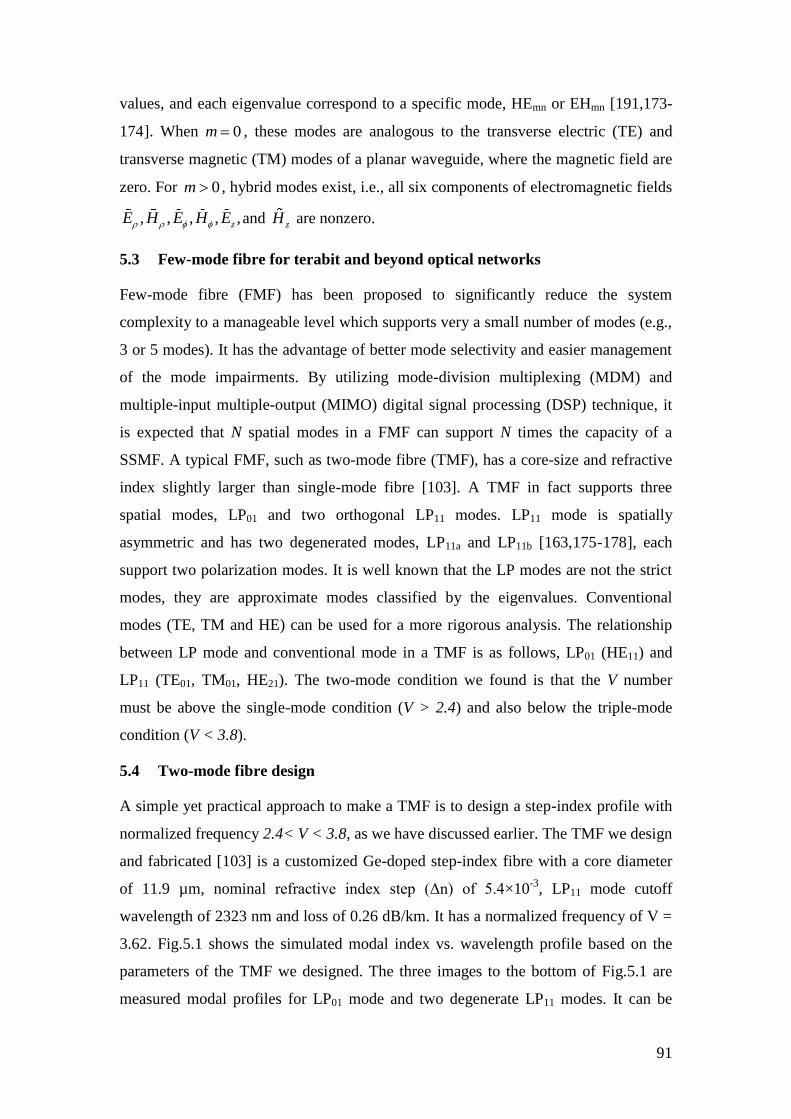
91
values, and each eigenvalue correspond to a specific mode, HEmn or EHmn [191,173-
174]. When 0m , these modes are analogous to the transverse electric (TE) and
transverse magnetic (TM) modes of a planar waveguide, where the magnetic field are
zero. For 0m , hybrid modes exist, i.e., all six components of electromagnetic fields
, , , , ,zE H E H E and zH are nonzero.
5.3 Few-mode fibre for terabit and beyond optical networks
Few-mode fibre (FMF) has been proposed to significantly reduce the system
complexity to a manageable level which supports very a small number of modes (e.g.,
3 or 5 modes). It has the advantage of better mode selectivity and easier management
of the mode impairments. By utilizing mode-division multiplexing (MDM) and
multiple-input multiple-output (MIMO) digital signal processing (DSP) technique, it
is expected that N spatial modes in a FMF can support N times the capacity of a
SSMF. A typical FMF, such as two-mode fibre (TMF), has a core-size and refractive
index slightly larger than single-mode fibre [103]. A TMF in fact supports three
spatial modes, LP01 and two orthogonal LP11 modes. LP11 mode is spatially
asymmetric and has two degenerated modes, LP11a and LP11b [163,175-178], each
support two polarization modes. It is well known that the LP modes are not the strict
modes, they are approximate modes classified by the eigenvalues. Conventional
modes (TE, TM and HE) can be used for a more rigorous analysis. The relationship
between LP mode and conventional mode in a TMF is as follows, LP01 (HE11) and
LP11 (TE01, TM01, HE21). The two-mode condition we found is that the V number
must be above the single-mode condition (V > 2.4) and also below the triple-mode
condition (V < 3.8).
5.4 Two-mode fibre design
A simple yet practical approach to make a TMF is to design a step-index profile with
normalized frequency 2.4< V < 3.8, as we have discussed earlier. The TMF we design
and fabricated [103] is a customized Ge-doped step-index fibre with a core diameter
of 11.9 µm, nominal refractive index step (Δn) of 5.4×10⁻³
, LP11 mode cutoff
wavelength of 2323 nm and loss of 0.26 dB/km. It has a normalized frequency of V =
3.62. Fig.5.1 shows the simulated modal index vs. wavelength profile based on the
parameters of the TMF we designed. The three images to the bottom of Fig.5.1 are
measured modal profiles for LP01 mode and two degenerate LP11 modes. It can be
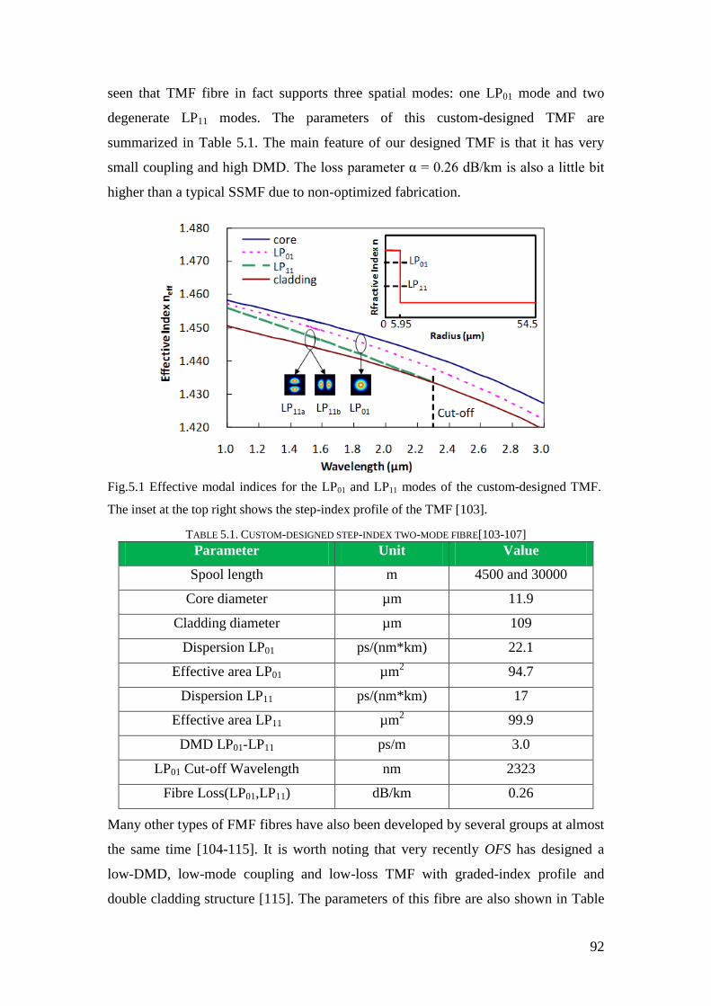
92
seen that TMF fibre in fact supports three spatial modes: one LP01 mode and two
degenerate LP11 modes. The parameters of this custom-designed TMF are
summarized in Table 5.1. The main feature of our designed TMF is that it has very
small coupling and high DMD. The loss parameter α = 0.26 dB/km is also a little bit
higher than a typical SSMF due to non-optimized fabrication.
Fig.5.1 Effective modal indices for the LP01 and LP11 modes of the custom-designed TMF.
The inset at the top right shows the step-index profile of the TMF [103].
TABLE 5.1. CUSTOM-DESIGNED STEP-INDEX TWO-MODE FIBRE[103-107]
Parameter Unit Value
Spool length m 4500 and 30000
Core diameter µm 11.9
Cladding diameter µm 109
Dispersion LP01 ps/(nm*km) 22.1
Effective area LP01 µm2
94.7
Dispersion LP11 ps/(nm*km) 17
Effective area LP11 µm2
99.9
DMD LP01-LP11 ps/m 3.0
LP01 Cut-off Wavelength nm 2323
Fibre Loss(LP01,LP11) dB/km 0.26
Many other types of FMF fibres have also been developed by several groups at almost
the same time [104-115]. It is worth noting that very recently OFS has designed a
low-DMD, low-mode coupling and low-loss TMF with graded-index profile and
double cladding structure [115]. The parameters of this fibre are also shown in Table
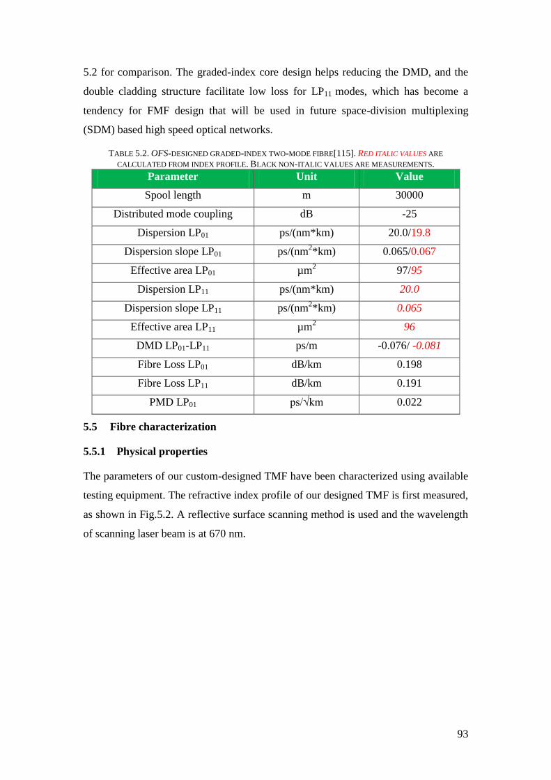
93
5.2 for comparison. The graded-index core design helps reducing the DMD, and the
double cladding structure facilitate low loss for LP11 modes, which has become a
tendency for FMF design that will be used in future space-division multiplexing
(SDM) based high speed optical networks.
TABLE 5.2. OFS-DESIGNED GRADED-INDEX TWO-MODE FIBRE[115]. RED ITALIC VALUES ARE
CALCULATED FROM INDEX PROFILE. BLACK NON-ITALIC VALUES ARE MEASUREMENTS.
Parameter Unit Value
Spool length m 30000
Distributed mode coupling dB -25
Dispersion LP01 ps/(nm*km) 20.0/19.8
Dispersion slope LP01 ps/(nm2*km) 0.065/0.067
Effective area LP01 µm2
97/95
Dispersion LP11 ps/(nm*km) 20.0
Dispersion slope LP11 ps/(nm2*km) 0.065
Effective area LP11 µm2
96
DMD LP01-LP11 ps/m -0.076/ -0.081
Fibre Loss LP01 dB/km 0.198
Fibre Loss LP11 dB/km 0.191
PMD LP01 ps/√km 0.022
5.5 Fibre characterization
5.5.1 Physical properties
The parameters of our custom-designed TMF have been characterized using available
testing equipment. The refractive index profile of our designed TMF is first measured,
as shown in Fig.5.2. A reflective surface scanning method is used and the wavelength
of scanning laser beam is at 670 nm.
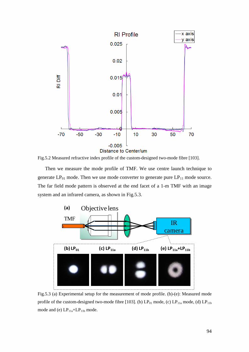
94
Fig.5.2 Measured refractive index profile of the custom-designed two-mode fibre [103].
Then we measure the mode profile of TMF. We use centre launch technique to
generate LP01 mode. Then we use mode converter to generate pure LP11 mode source.
The far field mode pattern is observed at the end facet of a 1-m TMF with an image
system and an infrared camera, as shown in Fig.5.3.
CCD
camera
TMFIR
camera
Objective lens
(b) LP01 (c) LP11a (d) LP11b (e) LP11a+LP11b
(a)
Fig.5.3 (a) Experimental setup for the measurement of mode profile. (b)-(e): Measured mode
profile of the custom-designed two-mode fibre [103]. (b) LP01 mode, (c) LP11a mode, (d) LP11b
mode and (e) LP11a+LP11b mode.
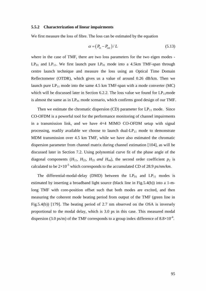
95
5.5.2 Characterization of linear impairments
We first measure the loss of fibre. The loss can be estimated by the equation
/in outP P L (5.13)
where in the case of TMF, there are two loss parameters for the two eigen modes -
LP01 and LP11. We first launch pure LP01 mode into a 4.5km TMF-span through
centre launch technique and measure the loss using an Optical Time Domain
Reflectometer (OTDR), which gives us a value of around 0.26 dB/km. Then we
launch pure LP11 mode into the same 4.5 km TMF-span with a mode converter (MC)
which will be discussed later in Section 6.2.2. The loss value we found for LP11mode
is almost the same as in LP01 mode scenario, which confirms good design of our TMF.
Then we estimate the chromatic dispersion (CD) parameter for LP11 mode. Since
CO-OFDM is a powerful tool for the performance monitoring of channel impairments
in a transmission link, and we have 4×4 MIMO CO-OFDM setup with signal
processing, readily available we choose to launch dual-LP11 mode to demonstrate
MDM transmission over 4.5 km TMF, while we have also estimated the chromatic
dispersion parameter from channel matrix during channel estimation [104], as will be
discussed later in Section 7.2. Using polynomial curve fit of the phase angle of the
diagonal components (H11, H22, H33 and H44), the second order coefficient p2 is
calculated to be 2×10⁻⁵
which corresponds to the accumulated CD of 28.9 ps/nm/km.
The differential-modal-delay (DMD) between the LP01 and LP11 modes is
estimated by inserting a broadband light source (black line in Fig.5.4(b)) into a 1-m-
long TMF with core-position offset such that both modes are excited, and then
measuring the coherent mode beating period from output of the TMF (green line in
Fig.5.4(b)) [179]. The beating period of 2.7 nm observed on the OSA is inversely
proportional to the modal delay, which is 3.0 ps in this case. This measured modal
dispersion (3.0 ps/m) of the TMF corresponds to a group index difference of 8.8×10⁻⁴
.
96
OSAASE
sourceOffset Butt
couplingOffset Splicing
TMFSMF SMF
In-line Polarizer
(a)
Before TMF
After TMF2.7nm
Wavelength (nm)
Before TMF
After TMF2.7nm
Wavelength (nm)
(b)
Fig.5.4 (a) Experimental setup for the measurement of DMD between LP01 and LP11 modes
through coherent beating. (b) Optical spectrum before (black line) and after (green line) a 1-
m-long TMF fibre measured with an OSA. The spectral power before TMF was scaled to be
in the same region as after TMF and does not reflect the real power level.
In addition, we have also estimated the mode beat length of our TMF. The
LP01/LP11 mode beat length is given by [176-178]
0 1 2 / BL (5.14)
The value of BL is first theoretically calculated using the refractive index profile of
our TMF and the result is 526 µm. Then we fabricate metal gratings which different
pitch size from 500~520 µm to make mode converters as will be discussed in Section
6.2.2. Maximum extinction ratio(ER) can be achieved when the grating pitch exactly
matches the beat length LB, which can be used as an indication of the real LB value. It
is found that LB is in the range of 510~520 µm at the wavelength of 1.55 µm. The
corresponding effective modal index difference effn is 2.98×10
-3, which agrees with
the calculation in Fig.5.1.

97
5.6 Conclusion
In this chapter, we show the design of the most basic but critical element in a space-
division multiplexing (SDM) system – few-mode fibre. First we have reviewed the
history and fundamentals of optical fibre and fibre modes. Then we show the
parameters of our custom-designed TMF. Finally the characterization of TMF is given
including physical properties and linear parameters. Our designed TMF has been used
in several proof-of-principle mode-division multiplexing (MDM) experiments
(Chapter 7), which shows the successful design and good quality.
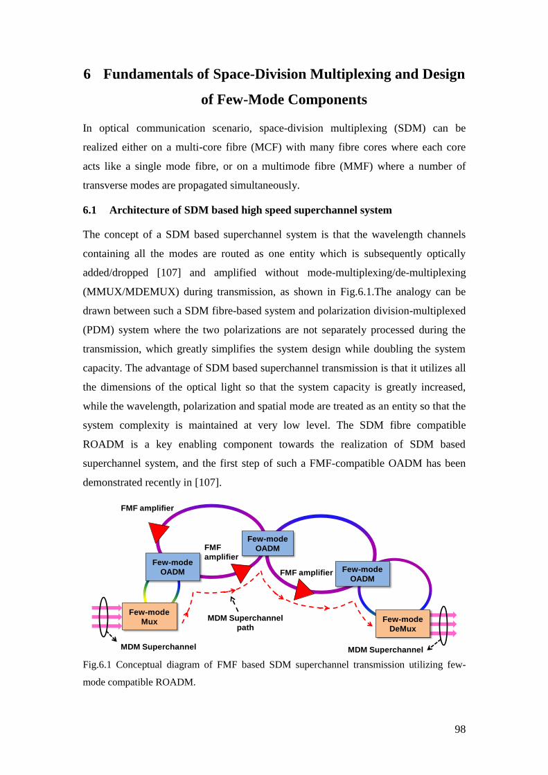
98
6 Fundamentals of Space-Division Multiplexing and Design
of Few-Mode Components
In optical communication scenario, space-division multiplexing (SDM) can be
realized either on a multi-core fibre (MCF) with many fibre cores where each core
acts like a single mode fibre, or on a multimode fibre (MMF) where a number of
transverse modes are propagated simultaneously.
6.1 Architecture of SDM based high speed superchannel system
The concept of a SDM based superchannel system is that the wavelength channels
containing all the modes are routed as one entity which is subsequently optically
added/dropped [107] and amplified without mode-multiplexing/de-multiplexing
(MMUX/MDEMUX) during transmission, as shown in Fig.6.1.The analogy can be
drawn between such a SDM fibre-based system and polarization division-multiplexed
(PDM) system where the two polarizations are not separately processed during the
transmission, which greatly simplifies the system design while doubling the system
capacity. The advantage of SDM based superchannel transmission is that it utilizes all
the dimensions of the optical light so that the system capacity is greatly increased,
while the wavelength, polarization and spatial mode are treated as an entity so that the
system complexity is maintained at very low level. The SDM fibre compatible
ROADM is a key enabling component towards the realization of SDM based
superchannel system, and the first step of such a FMF-compatible OADM has been
demonstrated recently in [107].
Few-mode
OADM
Few-mode
OADM
Few-mode
DeMux
Few-mode
OADM
Few-mode
Mux
FMF
amplifier
FMF amplifier
FMF amplifier
MDM Superchannel MDM Superchannel
MDM Superchannel
path
Fig.6.1 Conceptual diagram of FMF based SDM superchannel transmission utilizing few-
mode compatible ROADM.
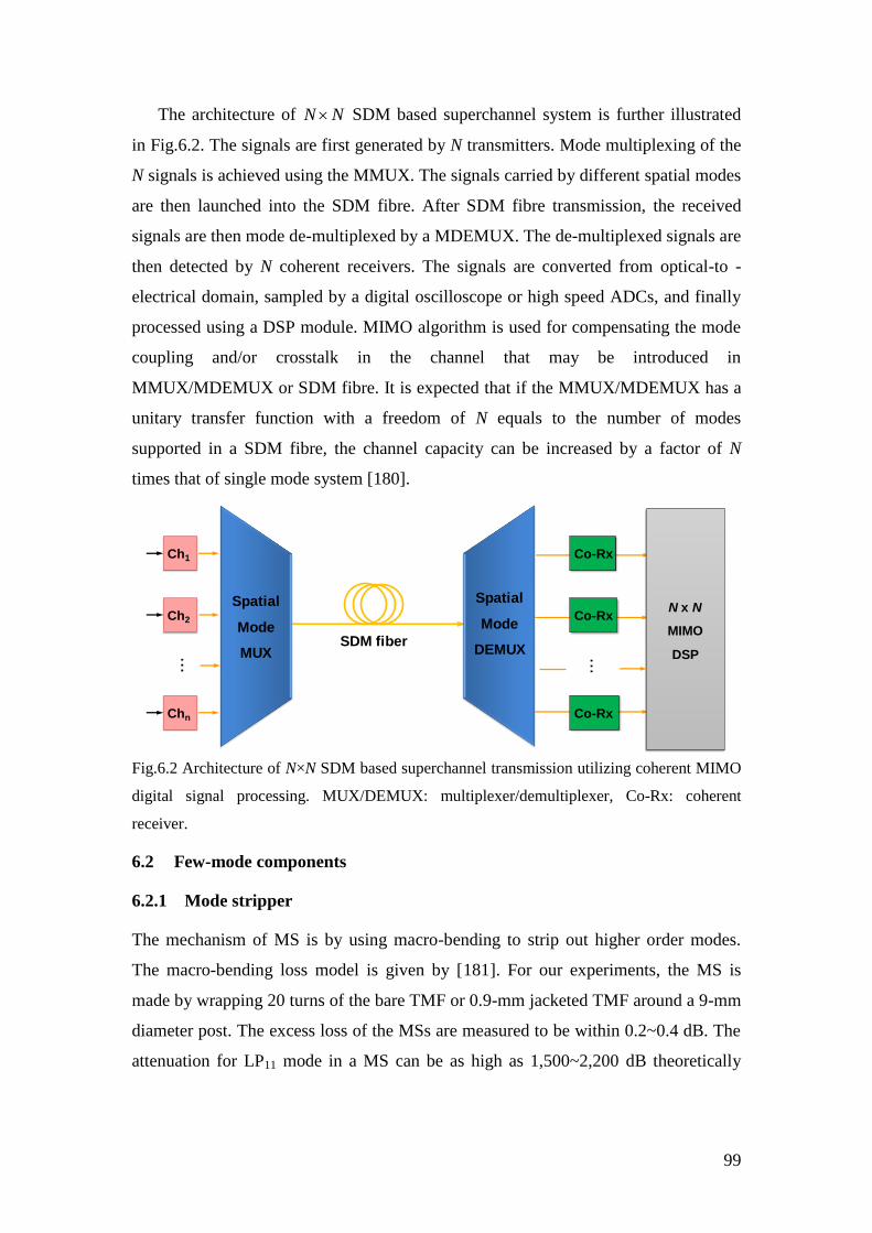
99
The architecture of N N SDM based superchannel system is further illustrated
in Fig.6.2. The signals are first generated by N transmitters. Mode multiplexing of the
N signals is achieved using the MMUX. The signals carried by different spatial modes
are then launched into the SDM fibre. After SDM fibre transmission, the received
signals are then mode de-multiplexed by a MDEMUX. The de-multiplexed signals are
then detected by N coherent receivers. The signals are converted from optical-to -
electrical domain, sampled by a digital oscilloscope or high speed ADCs, and finally
processed using a DSP module. MIMO algorithm is used for compensating the mode
coupling and/or crosstalk in the channel that may be introduced in
MMUX/MDEMUX or SDM fibre. It is expected that if the MMUX/MDEMUX has a
unitary transfer function with a freedom of N equals to the number of modes
supported in a SDM fibre, the channel capacity can be increased by a factor of N
times that of single mode system [180].
Ch1
Ch2
Chn
Co-Rx
Co-Rx
Co-Rx
N x N
MIMO
DSPSDM fiber
Spatial
Mode
MUX
Spatial
Mode
DEMUX...
...
Fig.6.2 Architecture of N×N SDM based superchannel transmission utilizing coherent MIMO
digital signal processing. MUX/DEMUX: multiplexer/demultiplexer, Co-Rx: coherent
receiver.
6.2 Few-mode components
6.2.1 Mode stripper
The mechanism of MS is by using macro-bending to strip out higher order modes.
The macro-bending loss model is given by [181]. For our experiments, the MS is
made by wrapping 20 turns of the bare TMF or 0.9-mm jacketed TMF around a 9-mm
diameter post. The excess loss of the MSs are measured to be within 0.2~0.4 dB. The
attenuation for LP11 mode in a MS can be as high as 1,500~2,200 dB theoretically
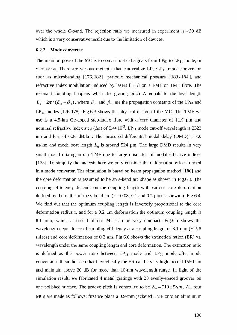
100
over the whole C-band. The rejection ratio we measured in experiment is ≥30 dB
which is a very conservative result due to the limitation of devices.
6.2.2 Mode converter
The main purpose of the MC is to convert optical signals from LP01 to LP11 mode, or
vice versa. There are various methods that can realize LP01/LP11 mode conversion
such as microbending [176, 182 ], periodic mechanical pressure [ 183 - 184 ], and
refractive index modulation induced by lasers [185] on a FMF or TMF fibre. The
resonant coupling happens when the grating pitch Λ equals to the beat length
01 112 / ( )BL , where 01 and 11 are the propagation constants of the LP01 and
LP11 modes [176-178]. Fig.6.3 shows the physical design of the MC. The TMF we
use is a 4.5-km Ge-doped step-index fibre with a core diameter of 11.9 µm and
nominal refractive index step (Δn) of 5.4×10⁻³
, LP11 mode cut-off wavelength is 2323
nm and loss of 0.26 dB/km. The measured differential-modal delay (DMD) is 3.0
ns/km and mode beat length BL is around 524 µm. The large DMD results in very
small modal mixing in our TMF due to large mismatch of modal effective indices
[178]. To simplify the analysis here we only consider the deformation effect formed
in a mode converter. The simulation is based on beam propagation method [186] and
the core deformation is assumed to be an s-bend arc shape as shown in Fig.6.3. The
coupling efficiency depends on the coupling length with various core deformation
defined by the radius of the s-bend arc (r = 0.08, 0.1 and 0.2 μm) is shown in Fig.6.4.
We find out that the optimum coupling length is inversely proportional to the core
deformation radius r, and for a 0.2 μm deformation the optimum coupling length is
8.1 mm, which assures that our MC can be very compact. Fig.6.5 shows the
wavelength dependence of coupling efficiency at a coupling length of 8.1 mm (~15.5
ridges) and core deformation of 0.2 μm. Fig.6.6 shows the extinction ration (ER) vs.
wavelength under the same coupling length and core deformation. The extinction ratio
is defined as the power ratio between LP11 mode and LP01 mode after mode
conversion. It can be seen that theoretically the ER can be very high around 1550 nm
and maintain above 20 dB for more than 10-nm wavelength range. In light of the
simulation result, we fabricated 4 metal gratings with 20 evenly-spaced grooves on
one polished surface. The groove pitch is controlled to be 0 510 5 m . All four
MCs are made as follows: first we place a 0.9-mm jacketed TMF onto an aluminium
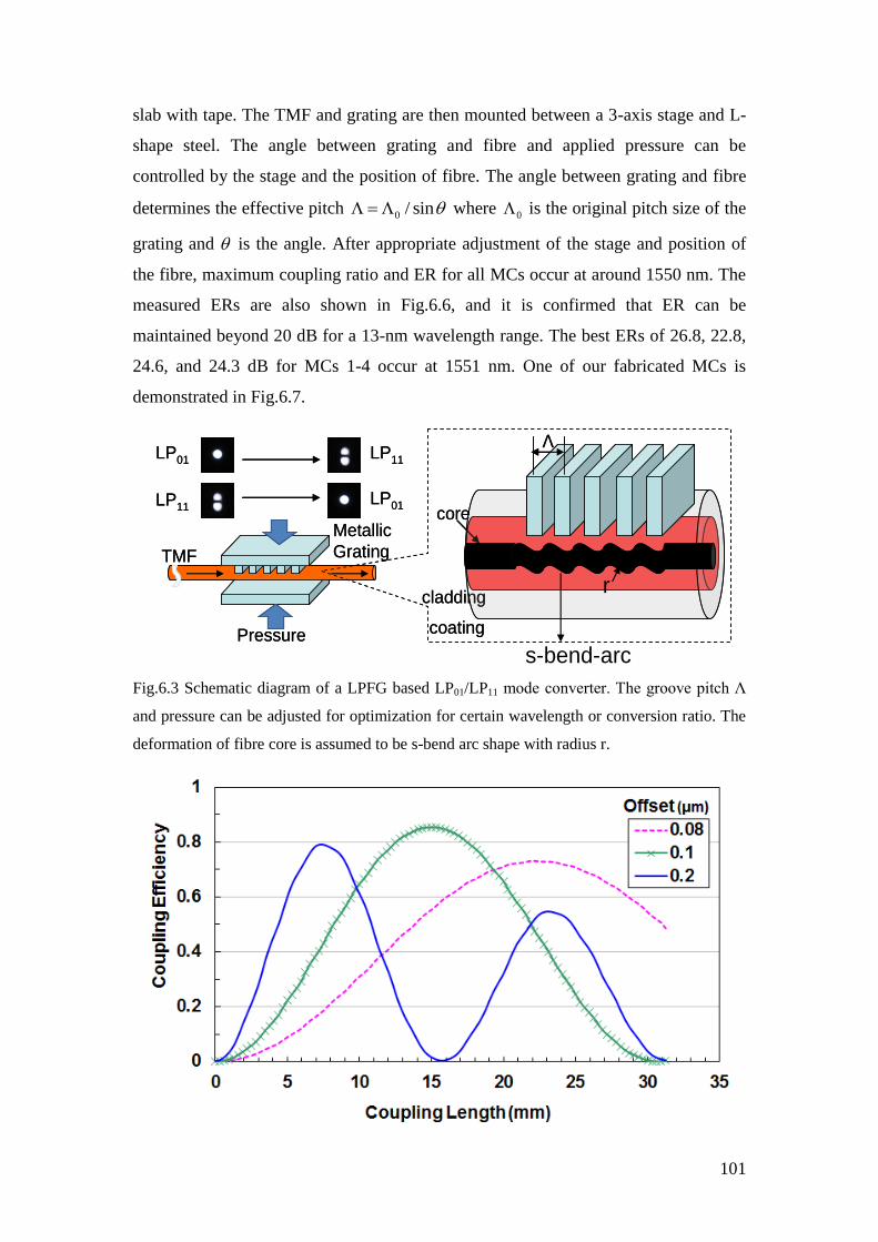
101
slab with tape. The TMF and grating are then mounted between a 3-axis stage and L-
shape steel. The angle between grating and fibre and applied pressure can be
controlled by the stage and the position of fibre. The angle between grating and fibre
determines the effective pitch 0 / sin where
0 is the original pitch size of the
grating and is the angle. After appropriate adjustment of the stage and position of
the fibre, maximum coupling ratio and ER for all MCs occur at around 1550 nm. The
measured ERs are also shown in Fig.6.6, and it is confirmed that ER can be
maintained beyond 20 dB for a 13-nm wavelength range. The best ERs of 26.8, 22.8,
24.6, and 24.3 dB for MCs 1-4 occur at 1551 nm. One of our fabricated MCs is
demonstrated in Fig.6.7.
TMF
LP01
LP11
LP11
LP01
Pressure
Metallic
Grating
core
cladding
coating
Λ
TMF
LP01
LP11
LP11
LP01
Pressure
Metallic
Grating
core
cladding
coating
Λ
s-bend-arc
r
Fig.6.3 Schematic diagram of a LPFG based LP01/LP11 mode converter. The groove pitch Λ
and pressure can be adjusted for optimization for certain wavelength or conversion ratio. The
deformation of fibre core is assumed to be s-bend arc shape with radius r.
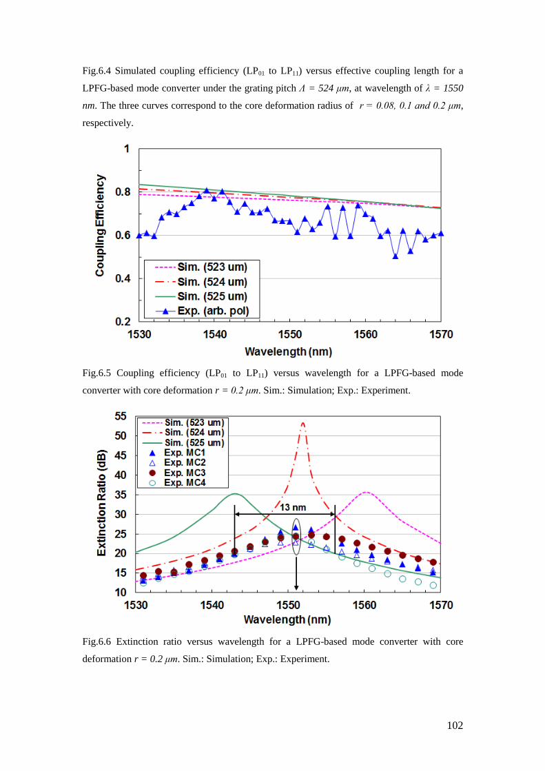
102
Fig.6.4 Simulated coupling efficiency (LP01 to LP11) versus effective coupling length for a
LPFG-based mode converter under the grating pitch Λ = 524 μm, at wavelength of λ = 1550
nm. The three curves correspond to the core deformation radius of r = 0.08, 0.1 and 0.2 μm,
respectively.
Fig.6.5 Coupling efficiency (LP01 to LP11) versus wavelength for a LPFG-based mode
converter with core deformation r = 0.2 μm. Sim.: Simulation; Exp.: Experiment.
Fig.6.6 Extinction ratio versus wavelength for a LPFG-based mode converter with core
deformation r = 0.2 μm. Sim.: Simulation; Exp.: Experiment.
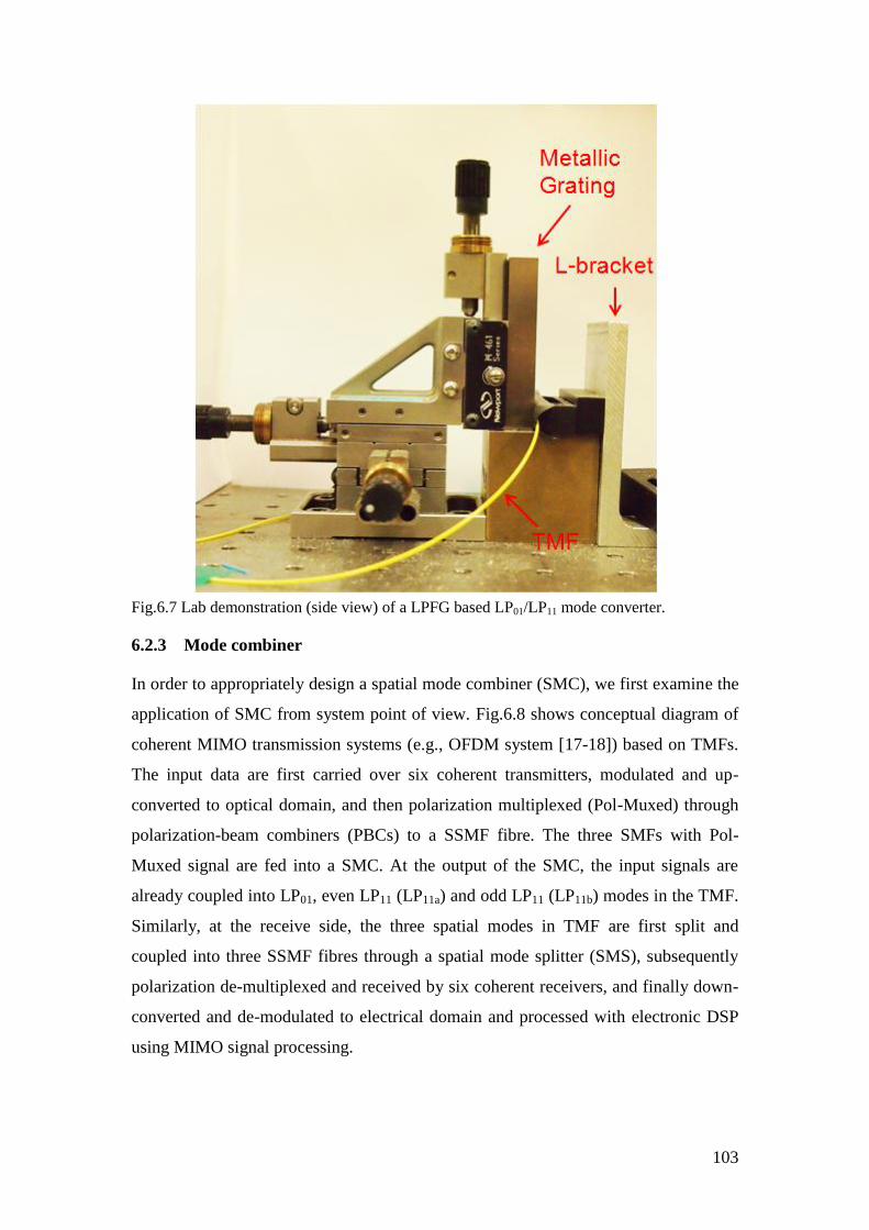
103
Fig.6.7 Lab demonstration (side view) of a LPFG based LP01/LP11 mode converter.
6.2.3 Mode combiner
In order to appropriately design a spatial mode combiner (SMC), we first examine the
application of SMC from system point of view. Fig.6.8 shows conceptual diagram of
coherent MIMO transmission systems (e.g., OFDM system [17-18]) based on TMFs.
The input data are first carried over six coherent transmitters, modulated and up-
converted to optical domain, and then polarization multiplexed (Pol-Muxed) through
polarization-beam combiners (PBCs) to a SSMF fibre. The three SMFs with Pol-
Muxed signal are fed into a SMC. At the output of the SMC, the input signals are
already coupled into LP01, even LP11 (LP11a) and odd LP11 (LP11b) modes in the TMF.
Similarly, at the receive side, the three spatial modes in TMF are first split and
coupled into three SSMF fibres through a spatial mode splitter (SMS), subsequently
polarization de-multiplexed and received by six coherent receivers, and finally down-
converted and de-modulated to electrical domain and processed with electronic DSP
using MIMO signal processing.
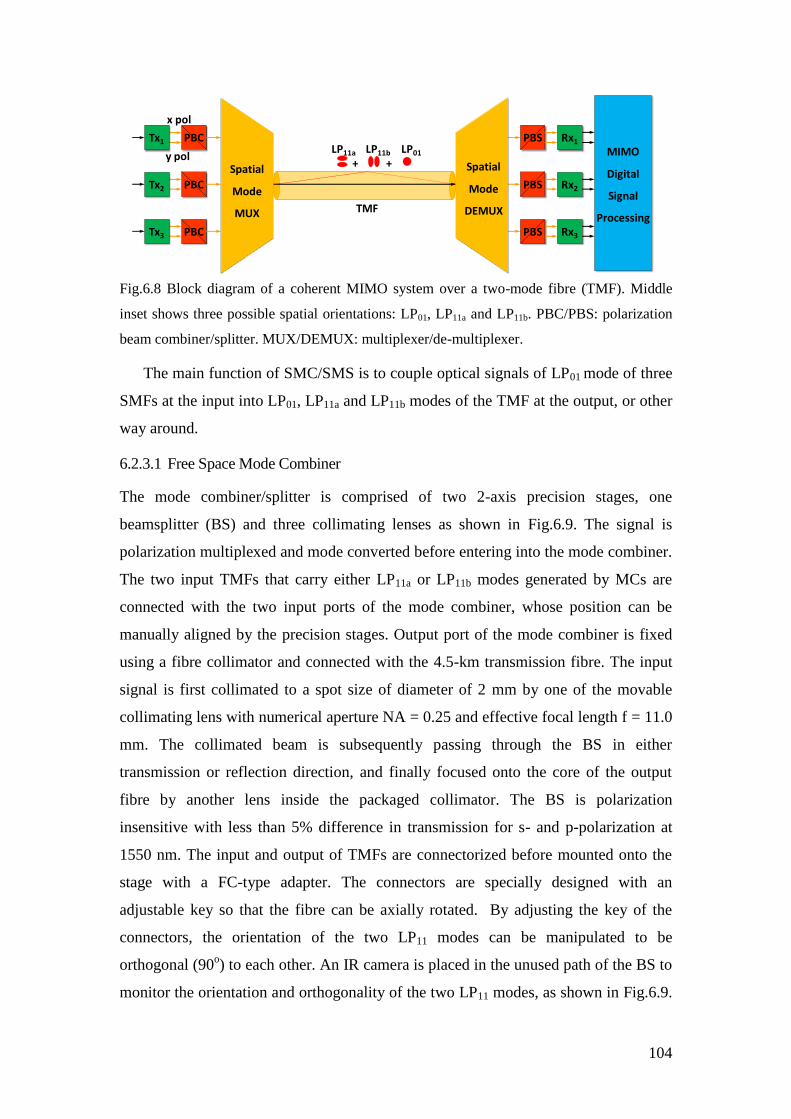
104
+ +MIMO
Digital
Signal
Processing
PBCTx1
PBCTx2
PBCTx3
TMF
x pol
y polLP01LP11bLP11a
PBS Rx1
PBS Rx2
PBS Rx3
Spatial
Mode
MUX
Spatial
Mode
DEMUX
Fig.6.8 Block diagram of a coherent MIMO system over a two-mode fibre (TMF). Middle
inset shows three possible spatial orientations: LP01, LP11a and LP11b. PBC/PBS: polarization
beam combiner/splitter. MUX/DEMUX: multiplexer/de-multiplexer.
The main function of SMC/SMS is to couple optical signals of LP01 mode of three
SMFs at the input into LP01, LP11a and LP11b modes of the TMF at the output, or other
way around.
6.2.3.1 Free Space Mode Combiner
The mode combiner/splitter is comprised of two 2-axis precision stages, one
beamsplitter (BS) and three collimating lenses as shown in Fig.6.9. The signal is
polarization multiplexed and mode converted before entering into the mode combiner.
The two input TMFs that carry either LP11a or LP11b modes generated by MCs are
connected with the two input ports of the mode combiner, whose position can be
manually aligned by the precision stages. Output port of the mode combiner is fixed
using a fibre collimator and connected with the 4.5-km transmission fibre. The input
signal is first collimated to a spot size of diameter of 2 mm by one of the movable
collimating lens with numerical aperture NA = 0.25 and effective focal length f = 11.0
mm. The collimated beam is subsequently passing through the BS in either
transmission or reflection direction, and finally focused onto the core of the output
fibre by another lens inside the packaged collimator. The BS is polarization
insensitive with less than 5% difference in transmission for s- and p-polarization at
1550 nm. The input and output of TMFs are connectorized before mounted onto the
stage with a FC-type adapter. The connectors are specially designed with an
adjustable key so that the fibre can be axially rotated. By adjusting the key of the
connectors, the orientation of the two LP11 modes can be manipulated to be
orthogonal (90o) to each other. An IR camera is placed in the unused path of the BS to
monitor the orientation and orthogonality of the two LP11 modes, as shown in Fig.6.9.
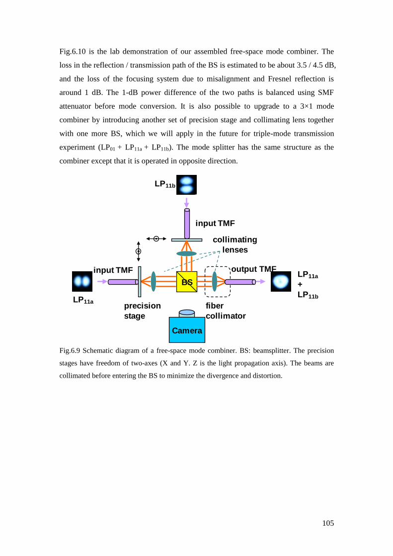
105
Fig.6.10 is the lab demonstration of our assembled free-space mode combiner. The
loss in the reflection / transmission path of the BS is estimated to be about 3.5 / 4.5 dB,
and the loss of the focusing system due to misalignment and Fresnel reflection is
around 1 dB. The 1-dB power difference of the two paths is balanced using SMF
attenuator before mode conversion. It is also possible to upgrade to a 3×1 mode
combiner by introducing another set of precision stage and collimating lens together
with one more BS, which we will apply in the future for triple-mode transmission
experiment (LP01 + LP11a + LP11b). The mode splitter has the same structure as the
combiner except that it is operated in opposite direction.
BS
precision
stage
fiber
collimator
collimating
lenses
LP11b
LP11a
LP11a
+
LP11b
output TMF
input TMF
input TMF
Camera
Fig.6.9 Schematic diagram of a free-space mode combiner. BS: beamsplitter. The precision
stages have freedom of two-axes (X and Y. Z is the light propagation axis). The beams are
collimated before entering the BS to minimize the divergence and distortion.
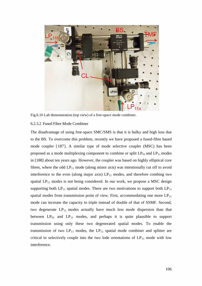
106
Fig.6.10 Lab demonstration (top view) of a free-space mode combiner.
6.2.3.2 Fused Fibre Mode Combiner
The disadvantage of using free-space SMC/SMS is that it is bulky and high loss due
to the BS. To overcome this problem, recently we have proposed a fused-fibre based
mode coupler [187]. A similar type of mode selective coupler (MSC) has been
proposed as a mode multiplexing component to combine or split LP01 and LP11 modes
in [188] about ten years ago. However, the coupler was based on highly elliptical core
fibres, where the odd LP11 mode (along minor axis) was intentionally cut off to avoid
interference to the even (along major axis) LP11 modes, and therefore combing two
spatial LP11 modes is not being considered. In our work, we propose a MSC design
supporting both LP11 spatial modes. There are two motivations to support both LP11
spatial modes from transmission point of view. First, accommodating one more LP11
mode can increase the capacity to triple instead of double of that of SSMF. Second,
two degenerate LP11 modes actually have much less mode dispersion than that
between LP01 and LP11 modes, and perhaps it is quite plausible to support
transmission using only these two degenerated spatial modes. To enable the
transmission of two LP11 modes, the LP11 spatial mode combiner and splitter are
critical to selectively couple into the two lode orientations of LP11 mode with low
interference.
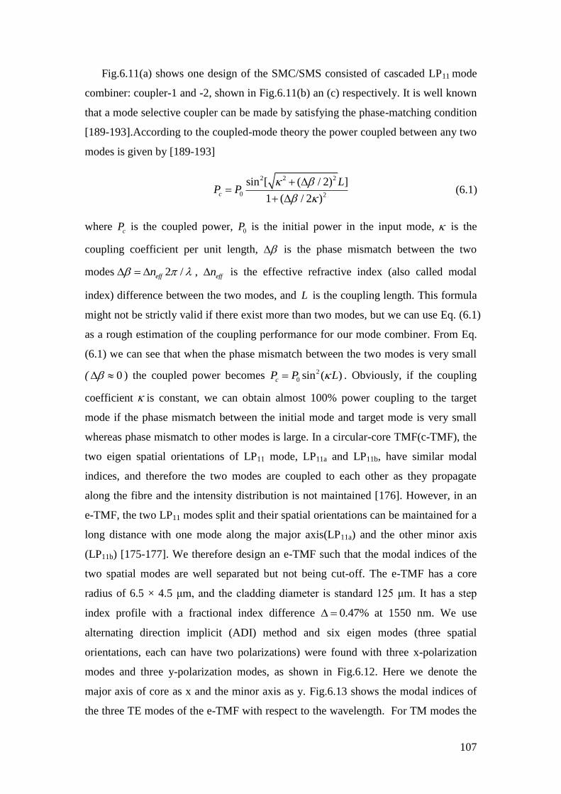
107
Fig.6.11(a) shows one design of the SMC/SMS consisted of cascaded LP11 mode
combiner: coupler-1 and -2, shown in Fig.6.11(b) an (c) respectively. It is well known
that a mode selective coupler can be made by satisfying the phase-matching condition
[189-193].According to the coupled-mode theory the power coupled between any two
modes is given by [189-193]
2 2 2
0 2
sin [ ( / 2) ]
1 ( / 2 )c
LP P
(6.1)
where cP is the coupled power, 0P is the initial power in the input mode, is the
coupling coefficient per unit length, is the phase mismatch between the two
modes 2 /effn , effn is the effective refractive index (also called modal
index) difference between the two modes, and L is the coupling length. This formula
might not be strictly valid if there exist more than two modes, but we can use Eq. (6.1)
as a rough estimation of the coupling performance for our mode combiner. From Eq.
(6.1) we can see that when the phase mismatch between the two modes is very small
( 0 ) the coupled power becomes 2
0 sin ( )cP P L . Obviously, if the coupling
coefficient is constant, we can obtain almost 100% power coupling to the target
mode if the phase mismatch between the initial mode and target mode is very small
whereas phase mismatch to other modes is large. In a circular-core TMF(c-TMF), the
two eigen spatial orientations of LP11 mode, LP11a and LP11b, have similar modal
indices, and therefore the two modes are coupled to each other as they propagate
along the fibre and the intensity distribution is not maintained [176]. However, in an
e-TMF, the two LP11 modes split and their spatial orientations can be maintained for a
long distance with one mode along the major axis(LP11a) and the other minor axis
(LP11b) [175-177]. We therefore design an e-TMF such that the modal indices of the
two spatial modes are well separated but not being cut-off. The e-TMF has a core
radius of 6.5 × 4.5 μm, and the cladding diameter is standard 125 μm. It has a step
index profile with a fractional index difference 0.47% at 1550 nm. We use
alternating direction implicit (ADI) method and six eigen modes (three spatial
orientations, each can have two polarizations) were found with three x-polarization
modes and three y-polarization modes, as shown in Fig.6.12. Here we denote the
major axis of core as x and the minor axis as y. Fig.6.13 shows the modal indices of
the three TE modes of the e-TMF with respect to the wavelength. For TM modes the
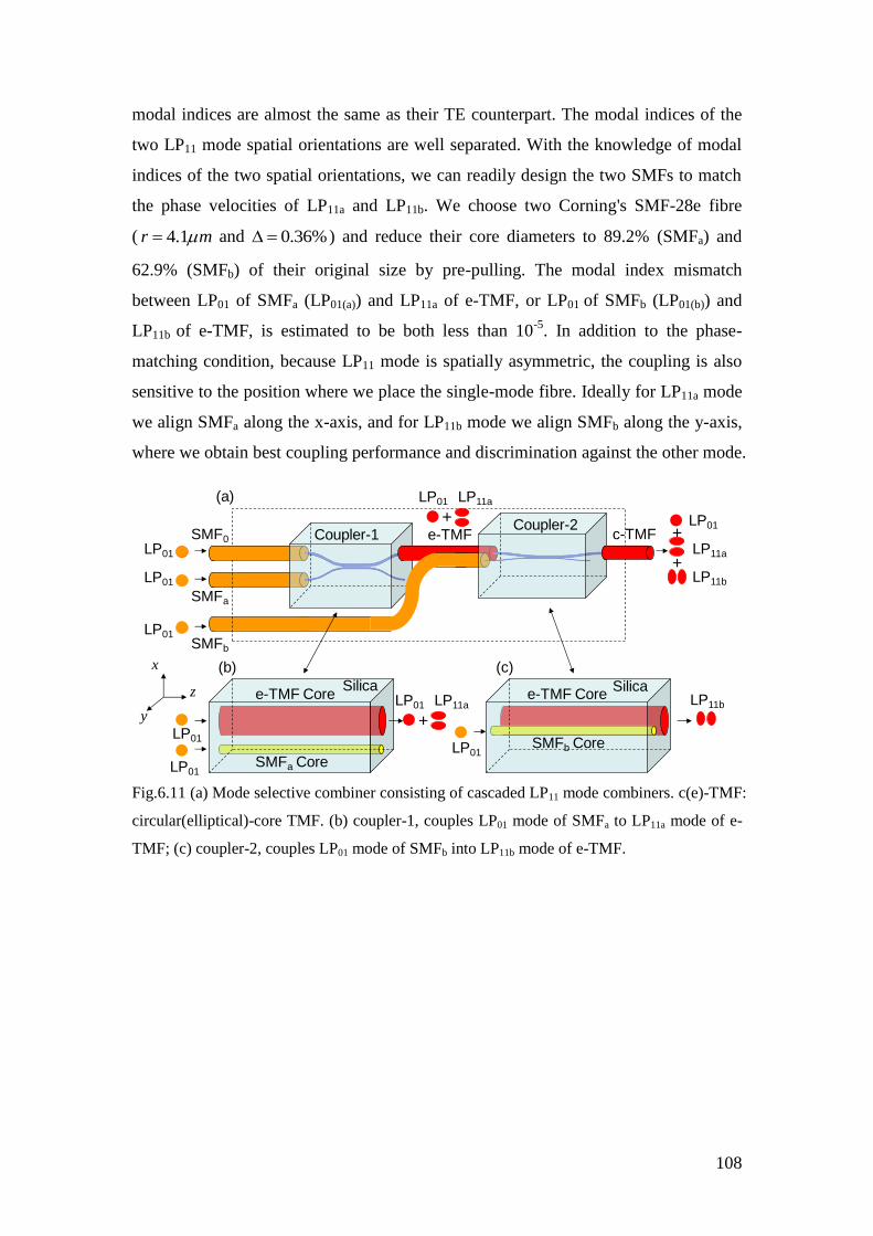
108
modal indices are almost the same as their TE counterpart. The modal indices of the
two LP11 mode spatial orientations are well separated. With the knowledge of modal
indices of the two spatial orientations, we can readily design the two SMFs to match
the phase velocities of LP11a and LP11b. We choose two Corning's SMF-28e fibre
( 4.1r m and 0.36% ) and reduce their core diameters to 89.2% (SMFa) and
62.9% (SMFb) of their original size by pre-pulling. The modal index mismatch
between LP01 of SMFa (LP01(a)) and LP11a of e-TMF, or LP01 of SMFb (LP01(b)) and
LP11b of e-TMF, is estimated to be both less than 10-5
. In addition to the phase-
matching condition, because LP11 mode is spatially asymmetric, the coupling is also
sensitive to the position where we place the single-mode fibre. Ideally for LP11a mode
we align SMFa along the x-axis, and for LP11b mode we align SMFb along the y-axis,
where we obtain best coupling performance and discrimination against the other mode.
SMFb
SMFa
SMF0 e-TMF c-TMF +
+
(c)
e-TMF Core
SMFa Core
SMFb Core
e-TMF Core
x
y
z SilicaSilica
(b)
(a)
LP01
LP01
LP01
LP01
LP01
LP01
LP11a
LP11b
LP11bLP11a
LP01
LP01
+
Coupler-1
LP11aLP01
+Coupler-2
Fig.6.11 (a) Mode selective combiner consisting of cascaded LP11 mode combiners. c(e)-TMF:
circular(elliptical)-core TMF. (b) coupler-1, couples LP01 mode of SMFa to LP11a mode of e-
TMF; (c) coupler-2, couples LP01 mode of SMFb into LP11b mode of e-TMF.
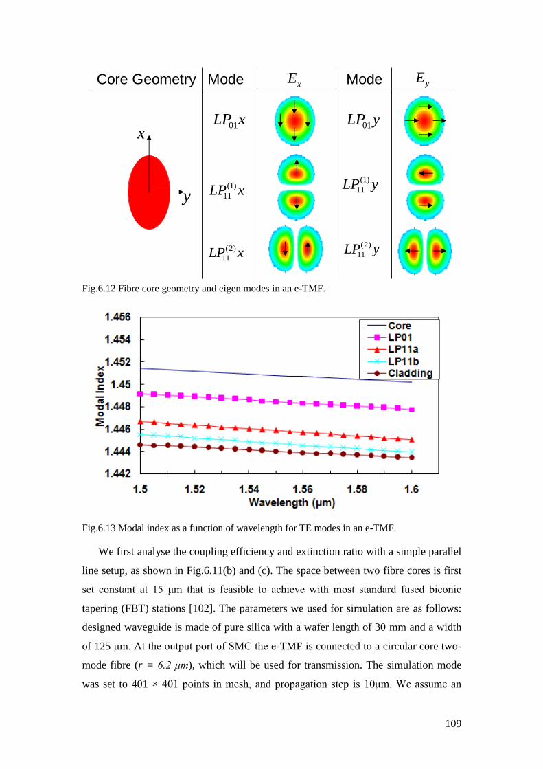
109
01LP x
(2)
11LP x
(1)
11LP x
xE yEMode
01LP y
(2)
11LP y
(1)
11LP y
ModeCore Geometry
x
y
Fig.6.12 Fibre core geometry and eigen modes in an e-TMF.
Fig.6.13 Modal index as a function of wavelength for TE modes in an e-TMF.
We first analyse the coupling efficiency and extinction ratio with a simple parallel
line setup, as shown in Fig.6.11(b) and (c). The space between two fibre cores is first
set constant at 15 μm that is feasible to achieve with most standard fused biconic
tapering (FBT) stations [102]. The parameters we used for simulation are as follows:
designed waveguide is made of pure silica with a wafer length of 30 mm and a width
of 125 μm. At the output port of SMC the e-TMF is connected to a circular core two-
mode fibre (r = 6.2 μm), which will be used for transmission. The simulation mode
was set to 401 × 401 points in mesh, and propagation step is 10μm. We assume an
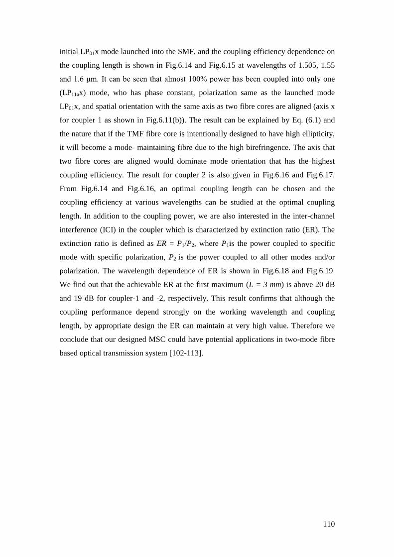
110
initial LP01x mode launched into the SMF, and the coupling efficiency dependence on
the coupling length is shown in Fig.6.14 and Fig.6.15 at wavelengths of 1.505, 1.55
and 1.6 μm. It can be seen that almost 100% power has been coupled into only one
(LP11ax) mode, who has phase constant, polarization same as the launched mode
LP01x, and spatial orientation with the same axis as two fibre cores are aligned (axis x
for coupler 1 as shown in Fig.6.11(b)). The result can be explained by Eq. (6.1) and
the nature that if the TMF fibre core is intentionally designed to have high ellipticity,
it will become a mode- maintaining fibre due to the high birefringence. The axis that
two fibre cores are aligned would dominate mode orientation that has the highest
coupling efficiency. The result for coupler 2 is also given in Fig.6.16 and Fig.6.17.
From Fig.6.14 and Fig.6.16, an optimal coupling length can be chosen and the
coupling efficiency at various wavelengths can be studied at the optimal coupling
length. In addition to the coupling power, we are also interested in the inter-channel
interference (ICI) in the coupler which is characterized by extinction ratio (ER). The
extinction ratio is defined as ER = P1/P2, where P1is the power coupled to specific
mode with specific polarization, P2 is the power coupled to all other modes and/or
polarization. The wavelength dependence of ER is shown in Fig.6.18 and Fig.6.19.
We find out that the achievable ER at the first maximum (L = 3 mm) is above 20 dB
and 19 dB for coupler-1 and -2, respectively. This result confirms that although the
coupling performance depend strongly on the working wavelength and coupling
length, by appropriate design the ER can maintain at very high value. Therefore we
conclude that our designed MSC could have potential applications in two-mode fibre
based optical transmission system [102-113].
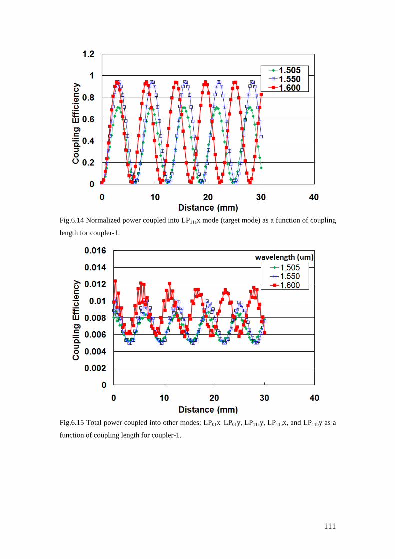
111
Fig.6.14 Normalized power coupled into LP11ax mode (target mode) as a function of coupling
length for coupler-1.
Fig.6.15 Total power coupled into other modes: LP01x, LP01y, LP11ay, LP11bx, and LP11by as a
function of coupling length for coupler-1.
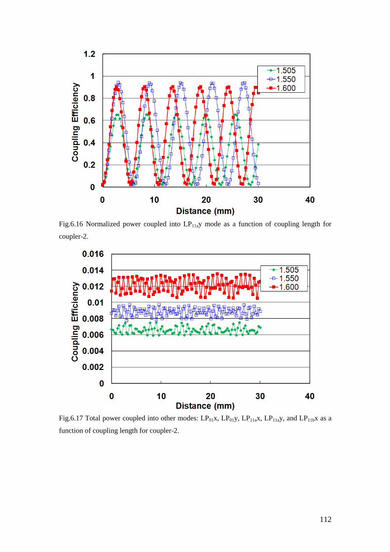
112
Fig.6.16 Normalized power coupled into LP11ay mode as a function of coupling length for
coupler-2.
Fig.6.17 Total power coupled into other modes: LP01x, LP01y, LP11ax, LP11ay, and LP11bx as a
function of coupling length for coupler-2.
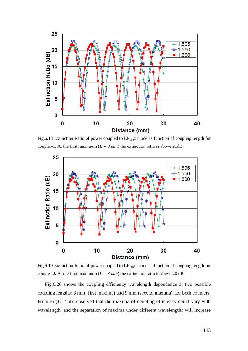
113
Fig.6.18 Extinction Ratio of power coupled to LP11ax mode as function of coupling length for
coupler-1. At the first maximum (L = 3 mm) the extinction ratio is above 21dB.
Fig.6.19 Extinction Ratio of power coupled to LP11bx mode as function of coupling length for
coupler-2. At the first maximum (L = 3 mm) the extinction ratio is above 20 dB.
Fig.6.20 shows the coupling efficiency wavelength dependence at two possible
coupling lengths: 3 mm (first maxima) and 9 mm (second maxima), for both couplers.
From Fig.6.14 it's observed that the maxima of coupling efficiency could vary with
wavelength, and the separation of maxima under different wavelengths will increase
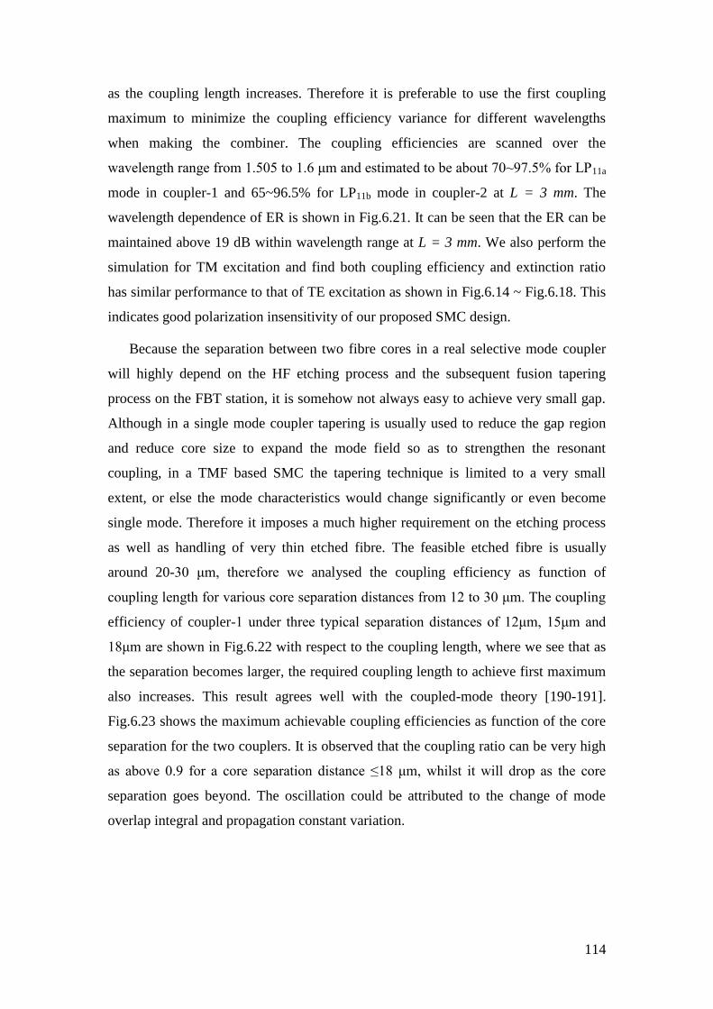
114
as the coupling length increases. Therefore it is preferable to use the first coupling
maximum to minimize the coupling efficiency variance for different wavelengths
when making the combiner. The coupling efficiencies are scanned over the
wavelength range from 1.505 to 1.6 μm and estimated to be about 70~97.5% for LP11a
mode in coupler-1 and 65~96.5% for LP11b mode in coupler-2 at L = 3 mm. The
wavelength dependence of ER is shown in Fig.6.21. It can be seen that the ER can be
maintained above 19 dB within wavelength range at L = 3 mm. We also perform the
simulation for TM excitation and find both coupling efficiency and extinction ratio
has similar performance to that of TE excitation as shown in Fig.6.14 ~ Fig.6.18. This
indicates good polarization insensitivity of our proposed SMC design.
Because the separation between two fibre cores in a real selective mode coupler
will highly depend on the HF etching process and the subsequent fusion tapering
process on the FBT station, it is somehow not always easy to achieve very small gap.
Although in a single mode coupler tapering is usually used to reduce the gap region
and reduce core size to expand the mode field so as to strengthen the resonant
coupling, in a TMF based SMC the tapering technique is limited to a very small
extent, or else the mode characteristics would change significantly or even become
single mode. Therefore it imposes a much higher requirement on the etching process
as well as handling of very thin etched fibre. The feasible etched fibre is usually
around 20-30 μm, therefore we analysed the coupling efficiency as function of
coupling length for various core separation distances from 12 to 30 μm. The coupling
efficiency of coupler-1 under three typical separation distances of 12μm, 15μm and
18μm are shown in Fig.6.22 with respect to the coupling length, where we see that as
the separation becomes larger, the required coupling length to achieve first maximum
also increases. This result agrees well with the coupled-mode theory [190-191].
Fig.6.23 shows the maximum achievable coupling efficiencies as function of the core
separation for the two couplers. It is observed that the coupling ratio can be very high
as above 0.9 for a core separation distance ≤18 μm, whilst it will drop as the core
separation goes beyond. The oscillation could be attributed to the change of mode
overlap integral and propagation constant variation.
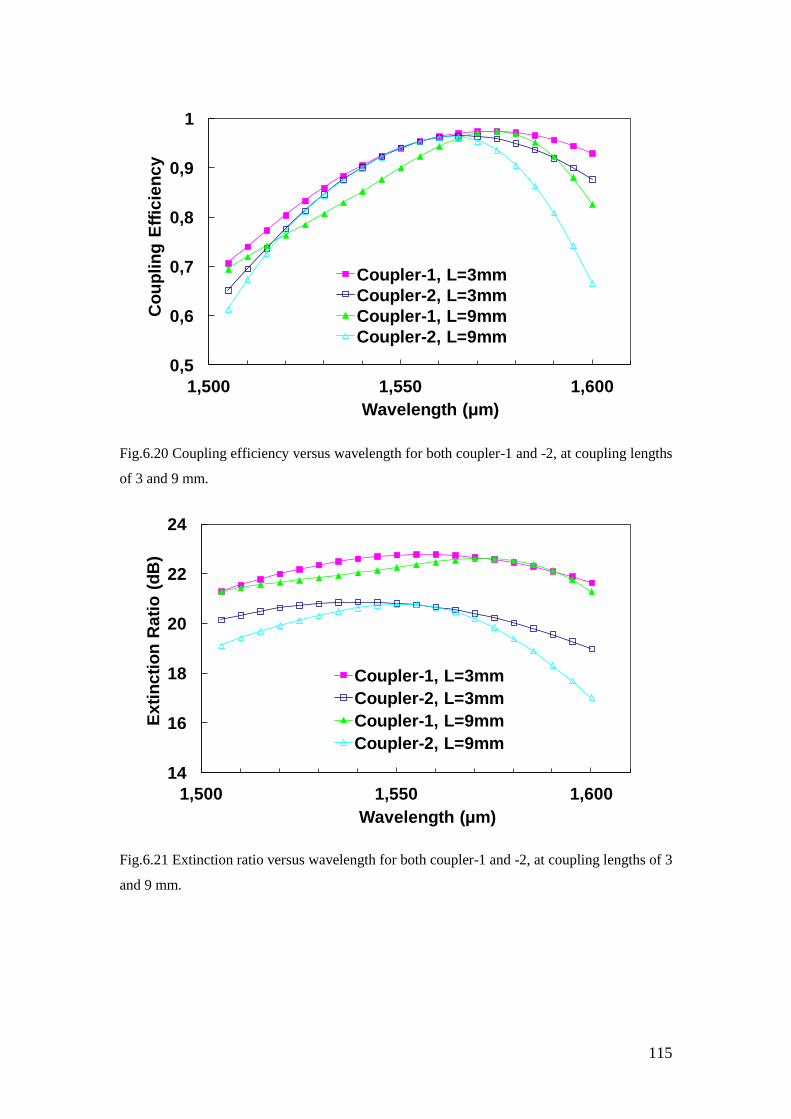
115
0,5
0,6
0,7
0,8
0,9
1
1,500 1,550 1,600
Co
up
lin
g E
ffic
ien
cy
Wavelength (μm)
Coupler-1, L=3mm
Coupler-2, L=3mm
Coupler-1, L=9mm
Coupler-2, L=9mm
Fig.6.20 Coupling efficiency versus wavelength for both coupler-1 and -2, at coupling lengths
of 3 and 9 mm.
14
16
18
20
22
24
1,500 1,550 1,600
Ex
tin
cti
on
Ra
tio
(d
B)
Wavelength (μm)
Coupler-1, L=3mm
Coupler-2, L=3mm
Coupler-1, L=9mm
Coupler-2, L=9mm
Fig.6.21 Extinction ratio versus wavelength for both coupler-1 and -2, at coupling lengths of 3
and 9 mm.
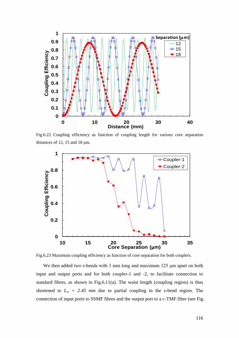
116
0
0.1
0.2
0.3
0.4
0.5
0.6
0.7
0.8
0.9
1
0 10 20 30 40
Co
up
lin
g E
ffic
ien
cy
Distance (mm)
12
15
18
Separation (m)
Fig.6.22 Coupling efficiency as function of coupling length for various core separation
distances of 12, 15 and 18 μm.
0
0.2
0.4
0.6
0.8
1
10 15 20 25 30 35
Co
up
lin
g E
ffic
ien
cy
Core Separation (μm)
Coupler-1
Coupler-2
Fig.6.23 Maximum coupling efficiency as function of core separation for both couplers.
We then added two s-bends with 3 mm long and maximum 125 μm apart on both
input and output ports and for both coupler-1 and -2, to facilitate connection to
standard fibres, as shown in Fig.6.11(a). The waist length (coupling region) is thus
shortened to Lw = 2.45 mm due to partial coupling in the s-bend region. The
connection of input ports to SSMF fibres and the output port to a c-TMF fibre (see Fig.
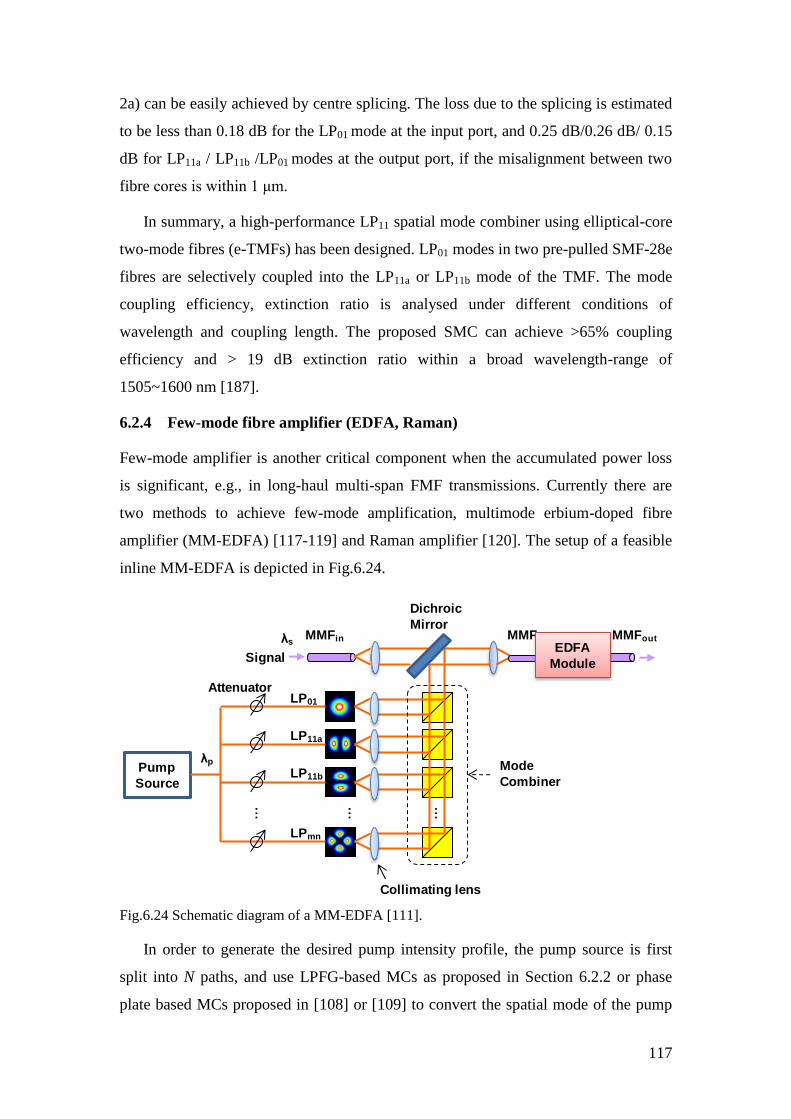
117
2a) can be easily achieved by centre splicing. The loss due to the splicing is estimated
to be less than 0.18 dB for the LP01 mode at the input port, and 0.25 dB/0.26 dB/ 0.15
dB for LP11a / LP11b /LP01 modes at the output port, if the misalignment between two
fibre cores is within 1 μm.
In summary, a high-performance LP11 spatial mode combiner using elliptical-core
two-mode fibres (e-TMFs) has been designed. LP01 modes in two pre-pulled SMF-28e
fibres are selectively coupled into the LP11a or LP11b mode of the TMF. The mode
coupling efficiency, extinction ratio is analysed under different conditions of
wavelength and coupling length. The proposed SMC can achieve >65% coupling
efficiency and > 19 dB extinction ratio within a broad wavelength-range of
1505~1600 nm [187].
6.2.4 Few-mode fibre amplifier (EDFA, Raman)
Few-mode amplifier is another critical component when the accumulated power loss
is significant, e.g., in long-haul multi-span FMF transmissions. Currently there are
two methods to achieve few-mode amplification, multimode erbium-doped fibre
amplifier (MM-EDFA) [117-119] and Raman amplifier [120]. The setup of a feasible
inline MM-EDFA is depicted in Fig.6.24.
MMFMMFin
Dichroic
Mirror
Mode
Combiner
……
LP01
LP11a
LP11b
LPmn
EDFA
Module
MMFout
Signal
Pump
Source
λp
λs
Attenuator
…
Collimating lens
Fig.6.24 Schematic diagram of a MM-EDFA [111].
In order to generate the desired pump intensity profile, the pump source is first
split into N paths, and use LPFG-based MCs as proposed in Section 6.2.2 or phase
plate based MCs proposed in [108] or [109] to convert the spatial mode of the pump
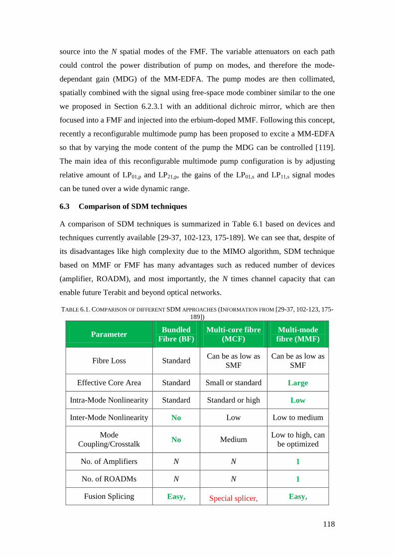
118
source into the N spatial modes of the FMF. The variable attenuators on each path
could control the power distribution of pump on modes, and therefore the mode-
dependant gain (MDG) of the MM-EDFA. The pump modes are then collimated,
spatially combined with the signal using free-space mode combiner similar to the one
we proposed in Section 6.2.3.1 with an additional dichroic mirror, which are then
focused into a FMF and injected into the erbium-doped MMF. Following this concept,
recently a reconfigurable multimode pump has been proposed to excite a MM-EDFA
so that by varying the mode content of the pump the MDG can be controlled [119].
The main idea of this reconfigurable multimode pump configuration is by adjusting
relative amount of LP01,p and LP21,p, the gains of the LP01,s and LP11,s signal modes
can be tuned over a wide dynamic range.
6.3 Comparison of SDM techniques
A comparison of SDM techniques is summarized in Table 6.1 based on devices and
techniques currently available [29-37, 102-123, 175-189]. We can see that, despite of
its disadvantages like high complexity due to the MIMO algorithm, SDM technique
based on MMF or FMF has many advantages such as reduced number of devices
(amplifier, ROADM), and most importantly, the N times channel capacity that can
enable future Terabit and beyond optical networks.
TABLE 6.1. COMPARISON OF DIFFERENT SDM APPROACHES (INFORMATION FROM [29-37, 102-123, 175-
189])
Parameter Bundled
Fibre (BF)
Multi-core fibre
(MCF)
Multi-mode
fibre (MMF)
Fibre Loss Standard Can be as low as
SMF
Can be as low as
SMF
Effective Core Area Standard Small or standard Large
Intra-Mode Nonlinearity Standard Standard or high Low
Inter-Mode Nonlinearity No Low Low to medium
Mode
Coupling/Crosstalk No Medium
Low to high, can
be optimized
No. of Amplifiers N N 1
No. of ROADMs N N 1
Fusion Splicing Easy, Special splicer, Easy,
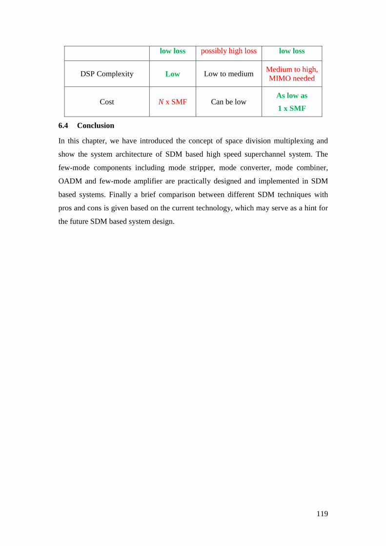
119
low loss possibly high loss low loss
DSP Complexity Low Low to medium Medium to high,
MIMO needed
Cost N x SMF Can be low As low as
1 x SMF
6.4 Conclusion
In this chapter, we have introduced the concept of space division multiplexing and
show the system architecture of SDM based high speed superchannel system. The
few-mode components including mode stripper, mode converter, mode combiner,
OADM and few-mode amplifier are practically designed and implemented in SDM
based systems. Finally a brief comparison between different SDM techniques with
pros and cons is given based on the current technology, which may serve as a hint for
the future SDM based system design.
120
7 Transmission of Mode-Division-Multiplexed CO-OFDM
(MDM-CO-OFDM) Signal over Two-Mode Fibre
7.1 Transmission of LP01/LP11 mode MDM-CO-OFDM signal over two-mode
fibre
In this experiment we have successfully achieved LP01/LP11 dual-mode transmission
over 4.5-km TMF [103], using the MSs and MCs as proposed in Section 6.2.1and
6.2.2.
7.1.1 System setup
The transmission experiment setup is as shown in Fig.7.1. Four transmitters are
emulated by polarization and mode multiplexing as follows: first, the transmitted
signal is generated off-line with MATLAB program. The total number of OFDM
subcarriers is 64, and cyclic prefix (CP) is set to be 1/8 of the observation window.
The middle 40 subcarriers out of 64 are filled with data mapped from 215
-1 PRBS.
500 OFDM symbols are sent for evaluation, out of which 20 symbols with alternative
polarization launch are used for channel estimation. The digital time-domain signal is
formed after IFFT operation. The real and imaginary components of the time-domain
signal are uploaded onto a Tektronix Arbitrary Waveform Generator (AWG). We
generate three optical tones spaced at 6.563GHz by feeding an external cavity laser at
1549.3 nm to two cascaded intensity modulators driven by RF tones at 6.563 GHz.
The baseband OFDM signal from AWG is impressed to the three optical tones by a
nested Mach-Zehnder modulator. The tone spacing is chosen to be an exact multiple
of the OFDM subcarrier spacing to ensure inter-band orthogonality. The orthogonally
multiplexed 3-band OFDM signal is then divided and recombined on orthogonal
polarizations with one symbol delay to emulate polarization multiplexing. The OFDM
symbol length is 7.2 ns. The raw data rate is 150 Gb/s and net data rate after deducting
all the overheads is 107 Gb/s for both modes and all 3 bands. The overheads include
7% forward error correction (FEC), 4% training symbol (TS), 12.5% CP and 5
discarded subcarriers around DC. The signal at a power of 5.5 dBm is then coupled
into the fibre with mode coupler MC1 to emulate the mode coupler. After a
transmission of 4.5-km TMF fibre, the mode delay is 13.5 ns. Since OFDM symbol is
7.2 ns, which is nearly half of the modal delay, the two modes are completely de-
correlated at the reception, validating the reception for two independent modes from
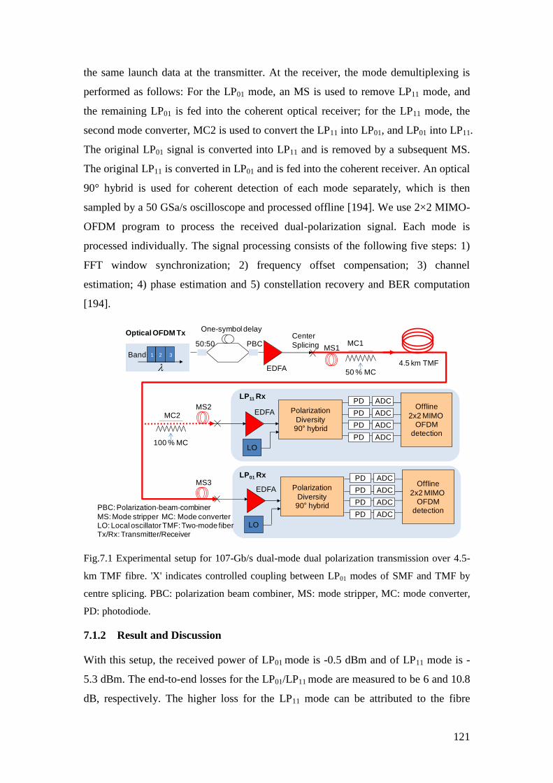
121
the same launch data at the transmitter. At the receiver, the mode demultiplexing is
performed as follows: For the LP01 mode, an MS is used to remove LP11 mode, and
the remaining LP01 is fed into the coherent optical receiver; for the LP11 mode, the
second mode converter, MC2 is used to convert the LP11 into LP01, and LP01 into LP11.
The original LP01 signal is converted into LP11 and is removed by a subsequent MS.
The original LP11 is converted in LP01 and is fed into the coherent receiver. An optical
90° hybrid is used for coherent detection of each mode separately, which is then
sampled by a 50 GSa/s oscilloscope and processed offline [194]. We use 2×2 MIMO-
OFDM program to process the received dual-polarization signal. Each mode is
processed individually. The signal processing consists of the following five steps: 1)
FFT window synchronization; 2) frequency offset compensation; 3) channel
estimation; 4) phase estimation and 5) constellation recovery and BER computation
[194].
PD
PD
PD
PD
Polarization
Diversity90 hybrid
LO
EDFA
ADC
ADC
ADC
ADC
Offline
2x2 MIMO OFDM
detection
PD
PD
PD
PD
Polarization
Diversity90 hybrid
LO
EDFA
ADC
ADC
ADC
ADC
Offline
2x2 MIMO OFDM
detection
4.5 km TMF
Center
Splicing
EDFA
One-symbol delay
50:50 PBC
50 % MC
100 % MC
MC1MS1
MC2MS2
MS3
LP11 Rx
Band: 1 2 3
Optical OFDM Tx
PBC: Polarization-beam-combiner
MS: Mode stripper MC: Mode converterLO: Local oscillator TMF: Two-mode fiberTx/Rx: Transmitter/Receiver
LP01 Rx
Fig.7.1 Experimental setup for 107-Gb/s dual-mode dual polarization transmission over 4.5-
km TMF fibre. 'X' indicates controlled coupling between LP01 modes of SMF and TMF by
centre splicing. PBC: polarization beam combiner, MS: mode stripper, MC: mode converter,
PD: photodiode.
7.1.2 Result and Discussion
With this setup, the received power of LP01 mode is -0.5 dBm and of LP11 mode is -
5.3 dBm. The end-to-end losses for the LP01/LP11 mode are measured to be 6 and 10.8
dB, respectively. The higher loss for the LP11 mode can be attributed to the fibre
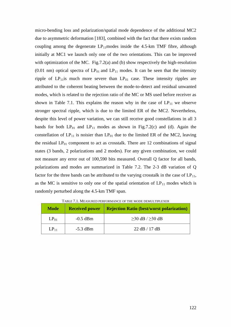
122
micro-bending loss and polarization/spatial mode dependence of the additional MC2
due to asymmetric deformation [183], combined with the fact that there exists random
coupling among the degenerate LP11modes inside the 4.5-km TMF fibre, although
initially at MC1 we launch only one of the two orientations. This can be improved
with optimization of the MC. Fig.7.2(a) and (b) show respectively the high-resolution
(0.01 nm) optical spectra of LP01 and LP11 modes. It can be seen that the intensity
ripple of LP11is much more severe than LP01 case. These intensity ripples are
attributed to the coherent beating between the mode-to-detect and residual unwanted
modes, which is related to the rejection ratio of the MC or MS used before receiver as
shown in Table 7.1. This explains the reason why in the case of LP11 we observe
stronger spectral ripple, which is due to the limited ER of the MC2. Nevertheless,
despite this level of power variation, we can still receive good constellations in all 3
bands for both LP01 and LP11 modes as shown in Fig.7.2(c) and (d). Again the
constellation of LP11 is noisier than LP01 due to the limited ER of the MC2, leaving
the residual LP01 component to act as crosstalk. There are 12 combinations of signal
states (3 bands, 2 polarizations and 2 modes). For any given combination, we could
not measure any error out of 100,590 bits measured. Overall Q factor for all bands,
polarizations and modes are summarized in Table 7.2. The 2-3 dB variation of Q
factor for the three bands can be attributed to the varying crosstalk in the case of LP11,
as the MC is sensitive to only one of the spatial orientation of LP11 modes which is
randomly perturbed along the 4.5-km TMF span.
TABLE 7.1. MEASURED PERFORMANCE OF THE MODE DEMULTIPLEXER
Mode Received power Rejection Ratio (best/worst polarization)
LP01 -0.5 dBm ≥30 dB / ≥30 dB
LP11 -5.3 dBm 22 dB / 17 dB
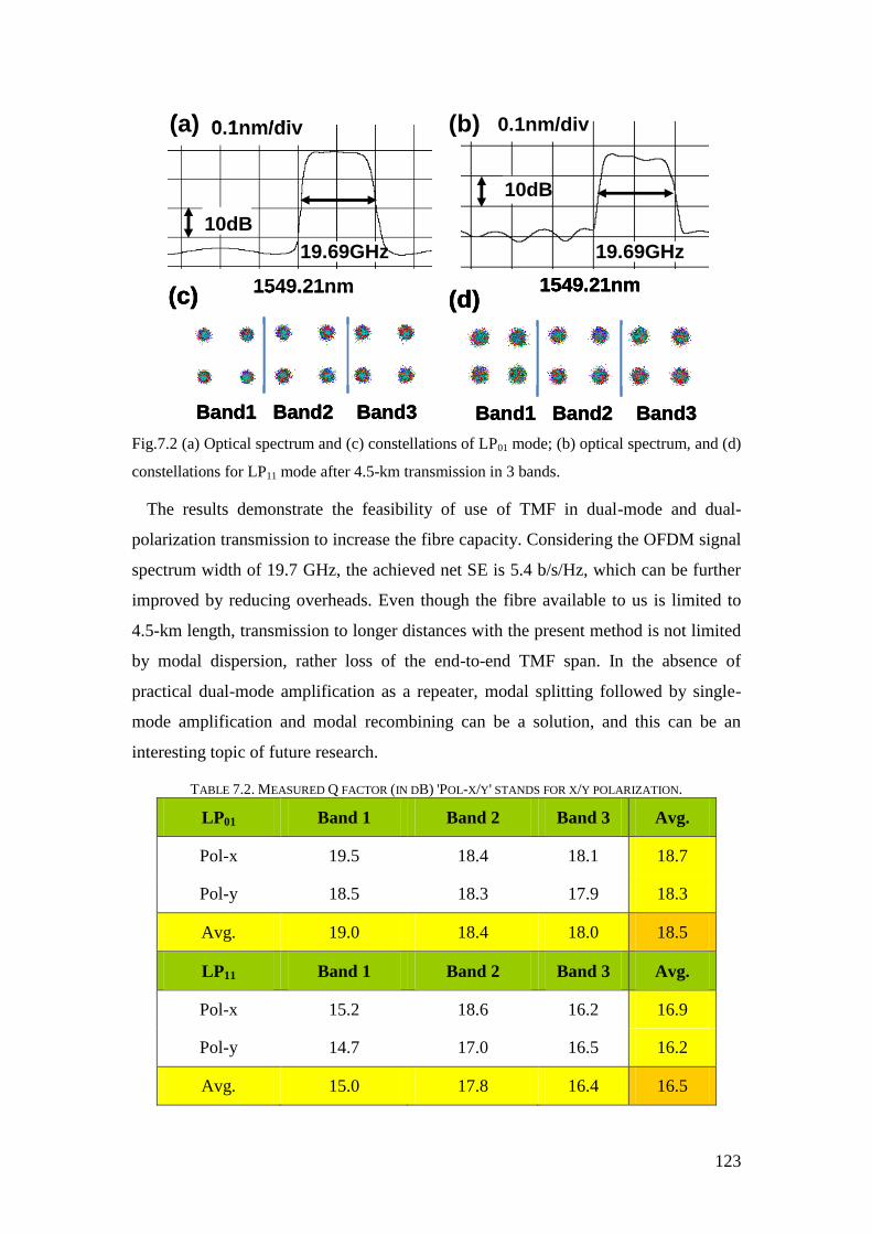
123
(a)
1549.21nm
0.1nm/div
19.69GHz
10dB
1549.21nm
(b) 0.1nm/div
19.69GHz
10dB
Band1 Band2 Band3
(c)
Band1 Band2 Band3
(d)
(a)
1549.21nm
0.1nm/div
19.69GHz
10dB
(a)
1549.21nm
0.1nm/div
19.69GHz
10dB
1549.21nm
(b) 0.1nm/div
19.69GHz
10dB
1549.21nm
(b) 0.1nm/div
19.69GHz
10dB
Band1 Band2 Band3
(c)
Band1 Band2 Band3
(c)
Band1 Band2 Band3
(d)
Band1 Band2 Band3
(d)
Fig.7.2 (a) Optical spectrum and (c) constellations of LP01 mode; (b) optical spectrum, and (d)
constellations for LP11 mode after 4.5-km transmission in 3 bands.
The results demonstrate the feasibility of use of TMF in dual-mode and dual-
polarization transmission to increase the fibre capacity. Considering the OFDM signal
spectrum width of 19.7 GHz, the achieved net SE is 5.4 b/s/Hz, which can be further
improved by reducing overheads. Even though the fibre available to us is limited to
4.5-km length, transmission to longer distances with the present method is not limited
by modal dispersion, rather loss of the end-to-end TMF span. In the absence of
practical dual-mode amplification as a repeater, modal splitting followed by single-
mode amplification and modal recombining can be a solution, and this can be an
interesting topic of future research.
TABLE 7.2. MEASURED Q FACTOR (IN DB) 'POL-X/Y' STANDS FOR X/Y POLARIZATION.
LP01 Band 1 Band 2 Band 3 Avg.
Pol-x 19.5 18.4 18.1 18.7
Pol-y 18.5 18.3 17.9 18.3
Avg. 19.0 18.4 18.0 18.5
LP11 Band 1 Band 2 Band 3 Avg.
Pol-x 15.2 18.6 16.2 16.9
Pol-y 14.7 17.0 16.5 16.2
Avg. 15.0 17.8 16.4 16.5
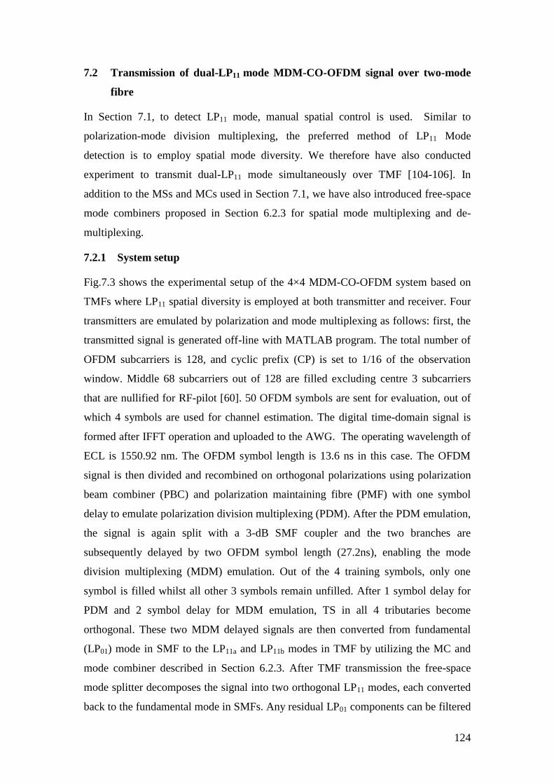
124
7.2 Transmission of dual-LP11 mode MDM-CO-OFDM signal over two-mode
fibre
In Section 7.1, to detect LP11 mode, manual spatial control is used. Similar to
polarization-mode division multiplexing, the preferred method of LP11 Mode
detection is to employ spatial mode diversity. We therefore have also conducted
experiment to transmit dual-LP11 mode simultaneously over TMF [104-106]. In
addition to the MSs and MCs used in Section 7.1, we have also introduced free-space
mode combiners proposed in Section 6.2.3 for spatial mode multiplexing and de-
multiplexing.
7.2.1 System setup
Fig.7.3 shows the experimental setup of the 4×4 MDM-CO-OFDM system based on
TMFs where LP11 spatial diversity is employed at both transmitter and receiver. Four
transmitters are emulated by polarization and mode multiplexing as follows: first, the
transmitted signal is generated off-line with MATLAB program. The total number of
OFDM subcarriers is 128, and cyclic prefix (CP) is set to 1/16 of the observation
window. Middle 68 subcarriers out of 128 are filled excluding centre 3 subcarriers
that are nullified for RF-pilot [60]. 50 OFDM symbols are sent for evaluation, out of
which 4 symbols are used for channel estimation. The digital time-domain signal is
formed after IFFT operation and uploaded to the AWG. The operating wavelength of
ECL is 1550.92 nm. The OFDM symbol length is 13.6 ns in this case. The OFDM
signal is then divided and recombined on orthogonal polarizations using polarization
beam combiner (PBC) and polarization maintaining fibre (PMF) with one symbol
delay to emulate polarization division multiplexing (PDM). After the PDM emulation,
the signal is again split with a 3-dB SMF coupler and the two branches are
subsequently delayed by two OFDM symbol length (27.2ns), enabling the mode
division multiplexing (MDM) emulation. Out of the 4 training symbols, only one
symbol is filled whilst all other 3 symbols remain unfilled. After 1 symbol delay for
PDM and 2 symbol delay for MDM emulation, TS in all 4 tributaries become
orthogonal. These two MDM delayed signals are then converted from fundamental
(LP01) mode in SMF to the LP11a and LP11b modes in TMF by utilizing the MC and
mode combiner described in Section 6.2.3. After TMF transmission the free-space
mode splitter decomposes the signal into two orthogonal LP11 modes, each converted
back to the fundamental mode in SMFs. Any residual LP01 components can be filtered
125
by mode converting to LP11 and then stripped off with the subsequent MSs. In this
experiment the MSs are realized by tightly winding the 0.9-mm jacketed TMF fibre
over 8-mm posts of about 10 rounds. After this, the two PDM tributaries are further
split to orthogonal polarizations by PBS and mixed with 4 LO branches using 3-dB
couplers into 4 photodetectors (PDs) with trans-impedance amplifiers. At receiver, we
choose heterodyne coherent detection so that only 4 PDs and one digital oscilloscope
with 4 channels of ADC are sufficient to realize the 4×4 MIMO reception.
Free-Space
Mode Splitter
1 symbol
delay
2 symbol
delay
PCs
WSSWSS
WSSWSS
LOLO
TMF
4x4 M
IMO
DS
P
4x4 M
IMO
DS
P
1550.9nm
ECL
laser
ECL
laser
MS1
MS2
BSBS
BS
3dB3dB
3dB3dB
3dB3dB
3dB3dB
1550.9nm
6dB6dB
PDPD
PDPD
PDPD
PDPD
ADCADC
ADCADC
ADCADC
ADCADC
MS3
MS4
MC1
MC2
MC3
MC4
3dB3dB
Free-Space
Mode Combiner
PBCPBCPBCPBC
Single Mode Fiber
Two Mode Fiber
Splicing Point and
Monitor Node
Single Mode Fiber
Two Mode Fiber
Splicing Point and
Monitor Node
PBSPBS
PBSPBS
EDFA
EDFA
EDFA
EDFA
AWGAWG
IQ Modulator
PM Fiber
Π/2
A
B
D
C
Fig.7.3 Experimental setup of a coherent 4×4-MIMO system over a two-mode fibre (TMF).
PBC/PBS: polarization beam combiner /splitter. MC: mode converter, MS: mode stripper.
WSS: wavelength selective switch, emulated by a Finisar waveshaper.
7.2.2 Result and Discussion
The optical power in the system is monitored at four nodes (A-D) as depicted in
Fig.7.3. The end-to-end loss is estimated for all the possible TX/RX port
combinations, as shown in Table 7.3. The relatively high power loss in our system is
mainly attributed to the loss of the beamsplitter (3.5-4.5 dB), misalignment/return loss
(~1 dB) and mode converter (1.4~2.4 dB). Nevertheless, the received power is well
above the sensitivity of PDs. Because of the relatively low differential mode delay
(DMD) between the two LP11 modes, the modal coupling happens even for a short
TMF fibre of 4.5 km due to random perturbation. The 4×4 MDM-CO-OFDM could
evaluate the channel matrix in the presence of polarization as well as mode coupling.
One of the estimated 4×4 channel matrices for the two LP11 modes after 4.5-km TMF
transmission is illustrated in Fig.7.4. A smooth channel response for a narrow
bandwidth is confirmed which shows slow frequency selectivity. Using polynomial
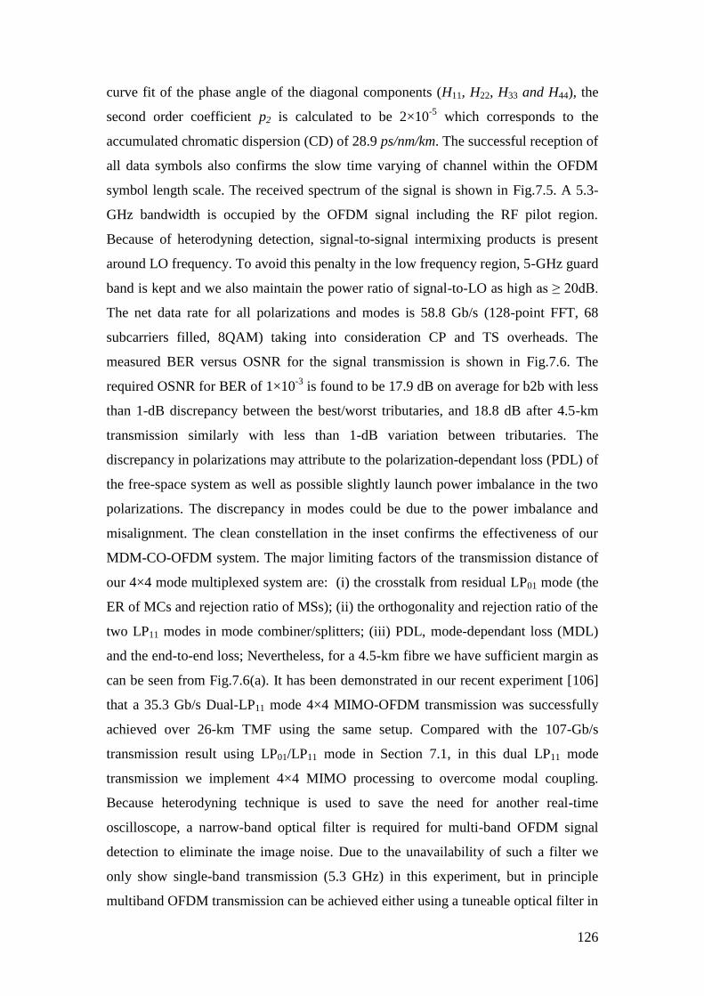
126
curve fit of the phase angle of the diagonal components (H11, H22, H33 and H44), the
second order coefficient p2 is calculated to be 2×10⁻⁵
which corresponds to the
accumulated chromatic dispersion (CD) of 28.9 ps/nm/km. The successful reception of
all data symbols also confirms the slow time varying of channel within the OFDM
symbol length scale. The received spectrum of the signal is shown in Fig.7.5. A 5.3-
GHz bandwidth is occupied by the OFDM signal including the RF pilot region.
Because of heterodyning detection, signal-to-signal intermixing products is present
around LO frequency. To avoid this penalty in the low frequency region, 5-GHz guard
band is kept and we also maintain the power ratio of signal-to-LO as high as ≥ 20dB.
The net data rate for all polarizations and modes is 58.8 Gb/s (128-point FFT, 68
subcarriers filled, 8QAM) taking into consideration CP and TS overheads. The
measured BER versus OSNR for the signal transmission is shown in Fig.7.6. The
required OSNR for BER of 1×10⁻³
is found to be 17.9 dB on average for b2b with less
than 1-dB discrepancy between the best/worst tributaries, and 18.8 dB after 4.5-km
transmission similarly with less than 1-dB variation between tributaries. The
discrepancy in polarizations may attribute to the polarization-dependant loss (PDL) of
the free-space system as well as possible slightly launch power imbalance in the two
polarizations. The discrepancy in modes could be due to the power imbalance and
misalignment. The clean constellation in the inset confirms the effectiveness of our
MDM-CO-OFDM system. The major limiting factors of the transmission distance of
our 4×4 mode multiplexed system are: (i) the crosstalk from residual LP01 mode (the
ER of MCs and rejection ratio of MSs); (ii) the orthogonality and rejection ratio of the
two LP11 modes in mode combiner/splitters; (iii) PDL, mode-dependant loss (MDL)
and the end-to-end loss; Nevertheless, for a 4.5-km fibre we have sufficient margin as
can be seen from Fig.7.6(a). It has been demonstrated in our recent experiment [106]
that a 35.3 Gb/s Dual-LP11 mode 4×4 MIMO-OFDM transmission was successfully
achieved over 26-km TMF using the same setup. Compared with the 107-Gb/s
transmission result using LP01/LP11 mode in Section 7.1, in this dual LP11 mode
transmission we implement 4×4 MIMO processing to overcome modal coupling.
Because heterodyning technique is used to save the need for another real-time
oscilloscope, a narrow-band optical filter is required for multi-band OFDM signal
detection to eliminate the image noise. Due to the unavailability of such a filter we
only show single-band transmission (5.3 GHz) in this experiment, but in principle
multiband OFDM transmission can be achieved either using a tuneable optical filter in
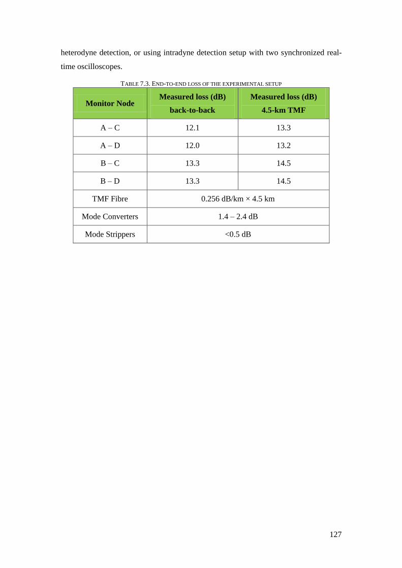
127
heterodyne detection, or using intradyne detection setup with two synchronized real-
time oscilloscopes.
TABLE 7.3. END-TO-END LOSS OF THE EXPERIMENTAL SETUP
Monitor Node Measured loss (dB)
back-to-back
Measured loss (dB)
4.5-km TMF
A – C 12.1 13.3
A – D 12.0 13.2
B – C 13.3 14.5
B – D 13.3 14.5
TMF Fibre 0.256 dB/km × 4.5 km
Mode Converters 1.4 – 2.4 dB
Mode Strippers <0.5 dB
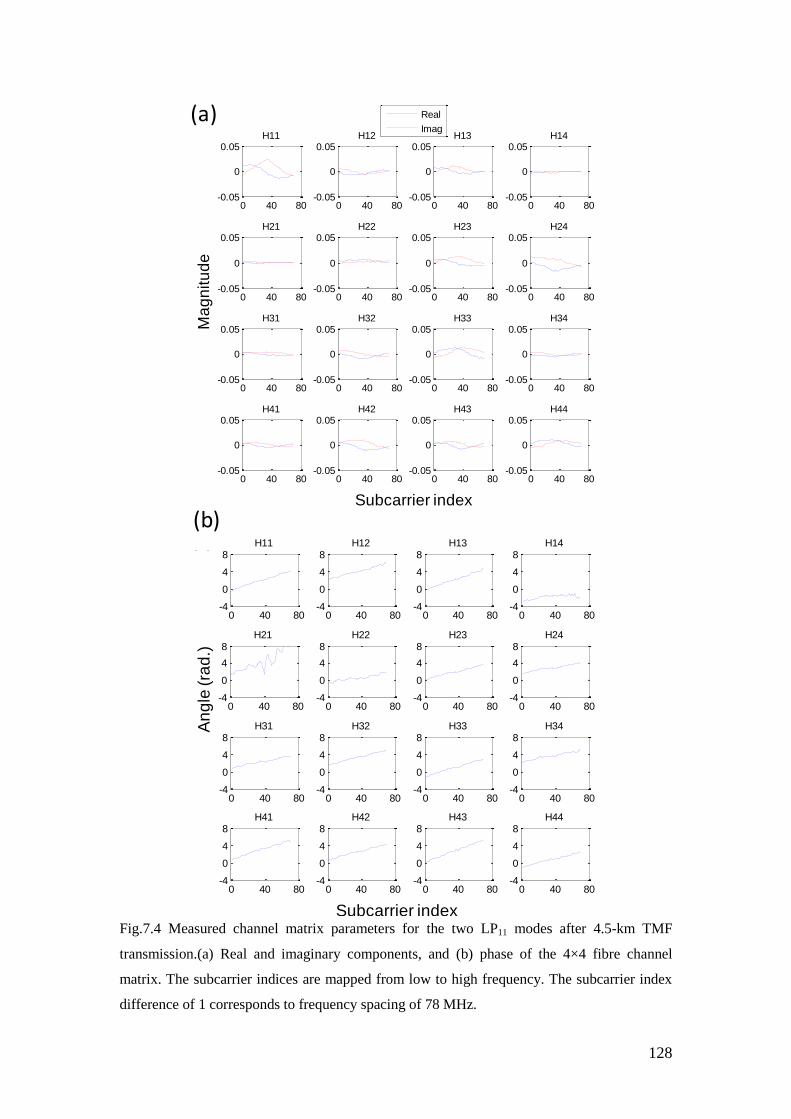
128
0 40 80-0.05
0
0.05H11
0 40 80-0.05
0
0.05H12
0 40 80-0.05
0
0.05H13
0 40 80-0.05
0
0.05H14
0 40 80-0.05
0
0.05H21
0 40 80-0.05
0
0.05H22
0 40 80-0.05
0
0.05H23
0 40 80-0.05
0
0.05H24
0 40 80-0.05
0
0.05H31
0 40 80-0.05
0
0.05H32
0 40 80-0.05
0
0.05H33
0 40 80-0.05
0
0.05H34
0 40 80-0.05
0
0.05H41
0 40 80-0.05
0
0.05H42
0 40 80-0.05
0
0.05H43
0 40 80-0.05
0
0.05H44
Real
Imag
Subcarrier index
Ma
gn
itu
de
(a)(a)
0 40 80-4
0
4
8H11
0 40 80-4
0
4
8H12
0 40 80-4
0
4
8H13
0 40 80-4
0
4
8H14
0 40 80-4
0
4
8H21
0 40 80-4
0
4
8H22
0 40 80-4
0
4
8H23
0 40 80-4
0
4
8H24
0 40 80-4
0
4
8H31
0 40 80-4
0
4
8H32
0 40 80-4
0
4
8H33
0 40 80-4
0
4
8H34
0 40 80-4
0
4
8H41
0 40 80-4
0
4
8H42
0 40 80-4
0
4
8H43
0 40 80-4
0
4
8H44
An
gle
(ra
d.)
(b)
Subcarrier index
(b)
Fig.7.4 Measured channel matrix parameters for the two LP11 modes after 4.5-km TMF
transmission.(a) Real and imaginary components, and (b) phase of the 4×4 fibre channel
matrix. The subcarrier indices are mapped from low to high frequency. The subcarrier index
difference of 1 corresponds to frequency spacing of 78 MHz.
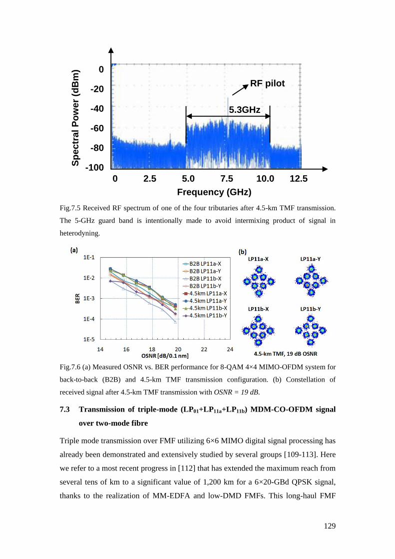
129
0 2.5 5.0 7.5 10.0 12.5
Frequency (GHz)
RF pilot
5.3GHz
0
-20
-40
-60
-80
-100Sp
ectr
al P
ow
er
(dB
m)
Fig.7.5 Received RF spectrum of one of the four tributaries after 4.5-km TMF transmission.
The 5-GHz guard band is intentionally made to avoid intermixing product of signal in
heterodyning.
Fig.7.6 (a) Measured OSNR vs. BER performance for 8-QAM 4×4 MIMO-OFDM system for
back-to-back (B2B) and 4.5-km TMF transmission configuration. (b) Constellation of
received signal after 4.5-km TMF transmission with OSNR = 19 dB.
7.3 Transmission of triple-mode (LP01+LP11a+LP11b) MDM-CO-OFDM signal
over two-mode fibre
Triple mode transmission over FMF utilizing 6×6 MIMO digital signal processing has
already been demonstrated and extensively studied by several groups [109-113]. Here
we refer to a most recent progress in [112] that has extended the maximum reach from
several tens of km to a significant value of 1,200 km for a 6×20-GBd QPSK signal,
thanks to the realization of MM-EDFA and low-DMD FMFs. This long-haul FMF
130
transmission is emulated by a triple-recirculating loop consists of three parallel routes
and switches, while a pair of spatial mode multiplexer (MMUX) and mode de-
multiplexer (MDEMUX) based on phase plates [108-110] are used before and after
the FMF span, enabling the loop control with single mode components. The longest
reach of up to 1,200 km is achieved at -3 dBm for 20% FEC limit (BER= 1×10⁻²
).
Due to the limited LP01/LP11 modal ER of our free-space mode combiner, however,
we did not achieve reasonable result for 6×6 MDM-CO-OFDM transmission of our
custom-designed TMF fibre, which we will investigate in the future. The
improvement can be made through either the optimization of our free-space mode
combiner setup, or the development of novel fused fibre mode coupler with high
modal ER [187-188].
7.4 Conclusion
In this chapter, we have shown our up-to-date proof-of-concept lab demonstrations of
transmission of MDM-CO-OFDM signal over TMF. Three different transmission
schemes are presented and discussed,
1) Transmission of LP01/LP11 mode MDM-CO-OFDM signal over 4.5-km two-
mode fibre.
2) Transmission of dual-LP11 mode MDM-CO-OFDM signal over 4.5-km two-mode
fibre using 8QAM modulation.
3) Transmission of triple (LP01+LP11a+LP11b) mode MDM-CO-OFDM signal over
two-mode fibre.
The system setup, key components, system parameters, enabling technique and signal
processing have been revealed.
131
8 Conclusions
8.1 Summary of this work
In this thesis, we have elucidated the overall system architecture and critical
components and sub-system modules for SDM transmission based on two-mode fibre
and presented the up-to-date experimental demonstration of MDM superchannel
transmission.
8.1.1 Novel variants of CO-OFDM system
We review the basic concept and principle of conventional Optical OFDM system.
We introduce two new variants of the Optical OFDM system called WPT-OFDM and
DFTS-OFDM. The system architecture, implementation and performance are
discussed.
8.1.2 Few-mode fibre and components for SDM
We focus on the most basic but important element for the SDM transmission system –
FMF fibre. The fundamentals of optical fibre and fibre modes are studied. We also
show how to design and fabricate a practical two-mode fibre. Furthermore, we have
conducted an experiment to characterize the physical property of our custom-designed
TMF fibre. After that we investigate the fundamentals of SDM especially the MDM
based on MMF or FMF. We show that despite of its disadvantage of high complexity
due to the MIMO algorithm, SDM technique based on MMF or FMF has many
advantages such as reduced number of devices (amplifier, ROADM), and most
importantly, N folds increase in channel capacity that facilitates future Terabit and
beyond optical networks. Finally, we show a few practical few-mode components
which are very critical for few-mode transmission such as mode stripper, mode
converter, mode combiner, optical add/drop multiplexer and few-mode amplifiers.
8.1.3 Transmission of MDM-CO-OFDM over Two-mode fibre
With few-mode components and subsystem modules available, the proof-of-concept
MDM transmission of CO-OFDM signal over FMF can be realised. We show three
experimental demonstrations of MDM transmission over TMF fibre: (1) transmission
of LP01/LP11 mode MDM-CO-OFDM signal, (2) transmission of dual-LP11 mode
MDM-CO-OFDM signal, and (3) transmission of triple-mode (LP01+LP11a+LP11b)
MDM-CO-OFDM signal over TMF fibre. We present a nonlinear propagation model
132
for the SDM transmission based on FMF fibre. The information spectral efficiency
and channel capacity of FMF based SDM system is derived, and a potential
improvement in the nonlinearity performance through constant linear mode coupling
is identified.
8.2 Future work and perspectives
It is expected that with the maturity of MDM and CO-OFDM superchannel technique,
a high data rate of 100 Gb/s and beyond can be achieved with doubled or even tripled
spectral efficiency over existing SMF systems. We identify the following critical
enabling components and modules for FMF transmission: low-loss and low-DMD
FMF [114], low-loss, high ER and all-fibre based mode MUX/DEMUX [102-113],
FMF compatible components (coupler [102,113,187], filter, switch, and ROADM
[107]), reliable parameter characterization(DMD, MDL, mode extinction/rejection
ratio, nonlinearity) devices, etc, which requires great effort to develop in the future.
There are also many other research directions: on the device level in terms of design
of low-loss few-mode components, design of few-mode amplifier with even less
mode dependence and flatter gain profile; on the system level in terms of multi-
dimensional coding, reduction of complexity in DSP algorithm, novel algorithm for
crosstalk and impairment mitigation, rigorous modelling of MDM transmission
system.
133
Bibliography
[1] A. G. Bell, "On the production and reproduction of sound by light," Am. J.
Sci., vol. 20, pp. 305–324 (1880).
[2] J. L. Baird, British Patent 285,738, (1928).
[3] C. W. Hansell, U. S. Patent 1,751,584, (1930).
[4] H. Lamm, "Biegsame optische gerate," Z. Instrumenten., vol. 50, pp. 579
(1930).
[5] A. C. S. van Heel, "A new method of transporting optical images without
aberrations," Nature, vol. 173, pp. 39 (1954).
[6] H. H. Hopkins and N. S. Kapany, "A flexible fiberscope using static
scanning," Nature, vol. 173, pp. 39–41 (1954).
[7] B. O’Brian, U. S. Patent 2,825,260 (1958).
[8] B. I. Hirschowitz, U. S. Patent 3,010,357 (1961).
[9] K. C. Kao and G. A. Hockham, "Dielectric-fiber surface waveguides for
optical frequencies," IEE Proc., vol. 113, pp. 1151 (1966).
[10] W. G. French, J. B. MacChesney, P. B. O’Connor, and G. W. Tasker, "Optical
Waveguides with Very Low Losses," Bell Syst. Tech. J., vol. 53, pp. 951
(1974).
[11] T. Miya, Y. Terunuma, T. Hosaka, and T. Miyashita, "Ultimate low-loss
single-mode fiber at 1.55 µm," Electron. Lett., vol. 15, no. 4, pp. 106–108
(1979).
[12] J. Hecht, City of Light, Oxford University Press, New York, USA, 1999.
[13] X. Zhu, and J.M. Kahn, "Free-space optical communication through
atmospheric turbulence channels," Communications, IEEE Transactions on,
vol. 50, no. 8, pp. 1293– 1300 (2002).
[14] D. Qian, M. Huang, E. Ip, Y. Huang, Y. Shao, J. Hu, and T. Wang, "101.7-
Tb/s (370×294-Gb/s) PDM-128QAM OFDM Transmission over 3×55-km
SSMF using Pilot-based Phase Noise Mitigation," in Optical Fiber
Communication Conference (OFC), 2011, paper PDPB5.
134
[15] A. Sano, T. Kobayashi, S. Yamanaka, A. Matsuura, H. Kawakami, Y.
Miyamoto, K. Ishihara, and H. Masuda,"102.3-Tb/s (224 x 548-Gb/s) C- and
Extended L-band All-Raman Transmission over 240 km Using PDM-64QAM
Single Carrier FDM with Digital Pilot Tone," in Optical Fiber Communication
Conference (OFC), 2012, paper PDP5C.3.
[16] S. Hara and R. Prasad, Multicarrier Techniques for 4G Mobile
Communications, Artech House, Boston, 2003.
[17] A. J. Lowery, L. Du, and J. Armstrong, "Orthogonal frequency division
multiplexing for adaptive dispersion compensation in long haul WDM
systems," in Optical Fiber Communication Conference (OFC), 2006, paper
PDP39.
[18] W. Shieh and C. Athaudage, "Coherent optical orthogonal frequency division
multiplexing," Electron. Lett., vol. 42, pp. 587–588 (2006).
[19] J. M. Tang, P. M. Lane, and K. A. Shore, “Transmission performance of
adaptively modulated optical OFDM signals in multimode fiber links,” IEEE
Photon. Technol. Lett., vol. 18, pp. 205–207 (2006).
[20] J. M. Tang, J.M., P.M. Lane, K. A. Shore, “30 Gb/s transmission over 40 km
directly modulated DFB laser-based SMF links without optical amplification
and dispersion compensation for VSR and metro applications,” in Optical
Fiber Communication Conference (OFC), 2006, paper JThB8.
[21] A. J. Lowery and J. Armstrong, "10 Gb/s multimode fiber link using power-
efficient orthogonal frequency-division multiplexing," Opt. Express, vol. 13,
pp. 10003-10009 (2005).
[22] I. B. Djordjevic and B. Vasic, "Orthogonal frequency division multiplexing for
high-speed optical transmission," Opt. Express, vol. 14, pp. 3767–3775 (2006).
[23] J. Armstrong, "OFDM for Optical Communications," J. Lightwave Technol.,
vol. 27, pp. 189–204 (2009).
[24] P. P. Mitra and J. B. Stark, "Nonlinear limits to the information capacity of
optical fiber communications," Nature, vol. 411, pp. 1027–1030 (2001).
135
[25] Ö. Bulakci, M. Schuster, C. Bunge, B. Spinnler, and N. Hanik, "Wavelet
transform based optical OFDM," in Optical Fiber Communication Conference
(OFC), 2009, paper OTUO6.
[26] 3rd Generation Partnership Project (3GPP). http://www.3gpp.org/LTE.
[27] K. Fazel and S. Kaiser, Multi-Carrier and Spread Spectrum Systems: From
OFDM and MC-CDMA to LTE and WiMAX, Second Edition, John Wiley &
Sons Ltd., Chichester, UK (2008).
[28] H. G. Myung, J. Lim, D. and J. Goodman, "Single carrier FDMA for uplink
wireless transmission," Vehicular Technology Magazine, IEEE, vol. 1, no. 3,
pp. 30–38 (2006).
[29] T. Hayashi, T. Taru, O. Shimakawa, T. Sasaki, and E. Sasaoka, "Ultra-Low-
Crosstalk Multi-Core Fiber Feasible to Ultra-Long-Haul Transmission," in
Optical Fiber Communication Conference (OFC), 2011, paper PDPC2.
[30] J. Sakaguchi, Y. Awaji, N. Wada, A. Kanno, T. Kawanishi, T. Hayashi, T.
Taru, T. Kobayashi, and M. Watanabe, "109-Tb/s (7×97×172-Gb/s
SDM/WDM/PDM) QPSK transmission through 16.8-km homogeneous multi-
core fiber," in Optical Fiber Communication Conference (OFC), 2011, paper
PDPB6.
[31] J. Sakaguchi, B.J. Puttnam, W. Klaus, Y. Awaji, N. Wada, A. Kanno, T.
Kawanishi, K. Imamura, H. Inaba, K. Mukasa, R. Sugizaki, T. Kobayashi, M.
Watanabe, "19-core fiber transmission of 19x100x172-Gb/s SDM-WDM-
PDM-QPSK signals at 305Tb/s," in Optical Fiber Communication Conference
(OFC), 2012, paper PDP5C.1.
[32] R. Ryf, R. Essiambre, A. Gnauch, S. Randel, M.A. Mestre, C. Schmidl, P.
Winzer, R. Delbue, P. Pupalaikis, A. Sureka, T. Hayashi, T. Taru, and T.
Sasaki, "Space-division Multiplexed Transmission over 4200 km 3-Core
mircrosctructured Fiber," in Optical Fiber Communication Conference (OFC),
2012, paper PDP5C.2.
[33] B. Zhu, T. Taunay, M. Fishteyn, X. Liu, S. Chandrasekhar, M. Yan, J. Fini, E.
Monberg, and F. Dimarcello, "Space-, Wavelength-, Polarization-Division
136
Multiplexed Transmission of 56-Tb/s over a 76.8-km Seven-Core Fiber," in
Optical Fiber Communication Conference (OFC), 2011, paper PDPB7.
[34] B. Zhu, T.F. Taunay, M. Fishteyn, X. Liu, S. Chandrasekhar, M. F. Yan, J. M.
Fini, E. M. Monberg, and F. V. Dimarcello, "112-Tb/s Space-division
multiplexed DWDM transmission with 14-b/s/Hz aggregate spectral efficiency
over a 76.8-km seven-core fiber," Opt. Express, vol. 19, pp. 16665–16671
(2011).
[35] S. Berdagué and P. Facq, "Mode division multiplexing in optical fibers," Appl.
Opt., vol. 21, pp. 1950–1955 (1982).
[36] H. R. Stuart, "Dispersive Multiplexing in Multimode Optical Fiber," Science,
vol. 289, pp. 281–283 (2000).
[37] B. C. Thomsen, "MIMO enabled 40 Gb/s transmission using mode division
multiplexing in multimode fiber," in Optical Fiber Communication
Conference (OFC), 2010, OThM6.
[38] B. Franz, D. Suikat, R. Dischler, F. Buchali, and H. Buelow, "High speed
OFDM data transmission over 5 km GI-multimode fiber using spatial
multiplexing with 2x4 MIMO processing," in European Conference and
Exhibition On Optical Communication (ECOC), 2010, paper Tu3.C.4.
[39] W. Shieh, H. Bao, and Y. Tang, "Coherent optical OFDM: theory and design,"
Opt. Express, vol. 16, pp. 841–859 (2008).
[40] Y. Ma, Q. Yang, Y. Tang, S. Chen, and W. Shieh, "1-Tb/s single-channel
coherent optical OFDM transmission over 600-km SSMF fiber with
subwavelength bandwidth access," Opt. Express, vol. 17, pp. 9421–9427
(2009).
[41] E. Yamada, A. Sano, and H. Masuda, "1Tb/s (111Gb/s/ch × 10ch) no-guard-
interval CO-OFDM transmission over 2100 km DSF," in Opto-Electronics and
Communications Conference, 2008 and the 2008 Australian Conference on
Optical Fiber Technology. OECC/ACOFT 2008. Joint conference of the,
paper PDP6.
[42] S. Chandrasekhar, X. Liu, B. Zhu, and D. W. Peckham, "Transmission of a
1.2-Tb/s 24-carrier no-guard-interval coherent OFDM superchannel over
137
7200-km of ultra-large-area fiber," in 35th European Conference on Optical
Communication (ECOC), 2009, vol. 2009-Supplement, no., pp.1–2, (2009).
[43] A. H. Gnauck, P. Winzer, C. Doerr, and L. Buhl, "10 x 112-Gb/s PDM 16-
QAM Transmission over 630 km of Fiber with 6.2-b/s/Hz Spectral
Efficiency," in Optical Fiber Communication Conference (OFC), 2009, paper
PDPB8.
[44] J. Yu, X. Zhou, M. F. Huang, Y. Shao, D. Qian, T.Wang, M. Cvijetic, P.
Magill, L. Nelson, M. Birk, S. Ten, H. B. Matthew, and S. K. Mishra, "17 Tb/s
(161x 114 Gb/s) PolMux-RZ-8PSK transmission over 662 km of ultra-low
loss fiber using C-band EDFA amplification and digital coherent detection," in
34th European Conference on Optical Communication (ECOC), 2008, paper
Th.3.E.2.
[45] A. Sano, H. Masuda, T. Kobayashi, M. Fujiwara, K. Horikoshi, E. Yoshida, Y.
Miyamoto, M. Matsui, M. Mizoguchi, H. Yamazaki, Y. Sakamaki, and H.
Ishii, "69.1-Tb/s (432 x 171-Gb/s) C- and Extended L-Band Transmission over
240 Km Using PDM-16-QAM Modulation and Digital Coherent Detection,"
in Optical Fiber Communication Conference (OFC), 2010, paper PDPB7.
[46] A. H. Gnauck, P. J. Winzer, S. Chandrasekhar, X. Liu, B. Zhu, and D. W.
Peckham, "10 x 224-Gb/s WDM transmission of 28-Gbaud PDM 16-QAM on
a 50-GHz grid over 1,200 km of fiber," in Optical Fiber Communication
Conference (OFC), 2012, paper PDPB8.
[47] X. Zhou, J. Yu, M. F. Huang, Y. Shao, T. Wang, L. Nelson, P. D. Magill, M.
Birk, P. I. Borel, D. W. Peckham, and R. Lingle, "64-Tb/s (640x 107-Gb/s)
PDM-36QAM transmission over 320 km using both pre- and post-
transmission digital equalization," in Optical Fiber Communication
Conference (OFC), 2010, paper PDPB9.
[48] Y.-K. Huang, E. Ip, M.-F. Huang, B. Zhu, P. N. Ji, Y. Shao, D. W. Peckham,
R. Lingle, Y. Aono, T. Tajima, and T. Wang, "10x456-Gb/s DP-16QAM
transmission over 8 x 100 km of ULAF using coherent detection with a 30-
GHz analog-to-digital converter,” in 15th OptoElectronics and
Communications Conference (OECC), Sapporo, Japan, Jul. 2010, paper PD3.
138
[49] M. S. Alfiad, M. Kuschnerov, S. L. Jansen, T. Wuth, D. van den Borne, and H.
de Waardt, "11 x 224-Gb/s POLMUX-RZ-16QAM transmission over 670 km
of SSMF with 50-GHz channel spacing," IEEE Photon. Technol. Lett., vol. 22,
no. 15, pp. 1150–1152 (2010).
[50] J.-X. Cai, Y. Cai, Y. Sun, C.R. Davidson, D.G. Foursa, A. Lucero, O. Sinkin,
W. Patterson, A. Pilipetskii, G. Mohs, and N.S. Bergano, "112x112 Gb/s
transmission over 9,360 km with channel spacing set to the baud rate (360%
spectral efficiency)," in 36th European Conference and Exposition on Optical
Communication (ECOC), 2010, paper PD2.1.
[51] M. Nölle, J. Hilt, L. Molle, M. Seimetz, and R. Freund, "8x224 Gbit/s PDM
16QAM WDM transmission with real-time signal processing at the
transmitter," in 36th European Conference and Exposition on Optical
Communication (ECOC), 2010, paper We.8.C.4.
[52] H. Ishio, J. Minowa and K. Nosu, "Review and status of wavelength-division-
multiplexing technology and its application," J. Lightwave Technol., vol. 2, no.
4, pp. 448-463 (1984).
[53] N. K. Cheung, K. Nosu and G. Winzer, Eds., "Special issue on dense
wavelength division multiplexing techniques for high capacity and multiple
access communication systems," IEEE J. Select. Areas Commun., vol. 8, no. 6,
pp. 945–1214 (1990).
[54] C. A. Brackett, "Dense Wavelength division multiplexing networks:
Principles and applications," IEEE J. Select. Areas Commun., vol. 8, no. 6, pp.
948–964 (1990).
[55] ITU-T Recommendation G.694.2, "WDM applications: CWDM wavelength
grid," (2003).
[56] A. D. Ellis and F. C. G. Gunning, “Spectral density enhancement using
coherent WDM,” IEEE Photon. Technol. Lett. 17, 504–506 (2005).
[57] T. Ohara, H. Takara, I. Shake, K. Mori, K. Sato, S. Kawanishi, S. Mino, T.
Yamada, M. Ishii, I. Ogawa, T. Kitoh, K. Magari, M. Okamoto, R. V. Roussev,
J. R. kurz, K. R. Parameswaran, and M. M. Fejer, "160-Gb/s OTDM
Transmission Using Integrated All-Optical MUX-DEMUX With All-Channel
139
Modulation and Demultiplexing," Photonics Technology Letters, IEEE, vol.
16, no. 2, pp. 650–652 (2004).
[58] W. Shieh, X. Yi, Y. Ma, and Y. Tang, "Theoretical and experimental study on
PMD-supported transmission using polarization diversity in coherent optical
OFDM systems," Optics Express, vol. 15, pp. 9936–9947 (2007).
[59] W. Shieh, X. Yi, and Y. Tang, "Transmission experiment of multi-gigabit
coherent optical OFDM systems over 1000 km SSMF fiber," Electron. Lett.,
vol. 43, 183–185 (2007).
[60] S. L. Jansen, I. Morita, N. Takeda, and H. Tanaka, "20-Gb/s OFDM
transmission over 4,160-km SSMF enabled by RF-Pilot tone phase noise
compensation," in Optical Fiber Communication Conference (OFC), 2007,
paper PDP15.
[61] Y. Tang, W. Shieh, X. Yi and R. Evans, "Optimum design for RF-to-optical
up-converter in coherent optical OFDM systems," IEEE Photon. Technol.
Lett., vol. 19, pp. 483–485 (2007).
[62] D. S. Ly-Gagnon, S. Tsukarnoto, K. Katoh, and K. Kikuchi, "Coherent
detection of optical quadrature phase-shift keying signals with carrier phase
estimation," J. Lightwave Technol., vol. 24, pp. 12–21, 2006.
[63] S. J. Savory, G. Gavioli, R. I. Killey, and P. Bayvel, "Electronic compensation
of chromatic dispersion using a digital coherent receiver," Optics Express, vol.
15, 2120–2126 (2007).
[64] S.B. Cohn and N.P. Weinhouse, "An automatic microwave phase
measurement system," Microwave Journal, vol. 7, pp. 49–56 (1964).
[65] C. A. Hoer and K.C. Roe, "Using an arbitrary six-port junction to measure
complex voltage ratios", IEEE Trans. on MTT, vol MTT-23, pp. 978–984
(1975).
[66] Y. Tang, W. Chen, W. Shieh, "Study of nonlinearity and dynamic range of
coherent optical OFDM receivers," in Optical Fiber Communication
Conference (OFC), 2008, paper JWA65.
[67] Q. Pan and R. J. Green, "Bit-error-rate performance of lightwave hybrid
AM/OFDM systems with comparison with AM/QAM systems in the presence
140
of clipping impulse noise," IEEE Photon. Technol. Lett., vol. 8, 278–280
(1996).
[68] A. J. Lowery and J. Armstrong, "Orthogonal-frequency-division multiplexing
for dispersion compensation of long-haul optical systems," Optics Express, vol.
14, no. 6, pp. 2079–2084 (2006).
[69] J. M. Tang and K. A. Shore, "Maximizing the transmission performance of
adaptively modulated optical OFDM signals in multimode-fiber links by
optimizing analog-to-digital converters," J. Lightwave Technol., vol. 25, pp.
787–798 (2007).
[70] X. Q. Jin, J. M. Tang, P. S. Spencer, and K. A. Shore, "Optimization of
adaptively modulated optical OFDM modems for multimode fiber-based local
area networks," J. Opt. Networking, vol. 7, pp. 198–214, (2008).
[71] B. J. C. Schmidt, A. J. Lowery and J. Armstrong, "Experimental
demonstrations of 20 Gbit/s direct-detection optical OFDM and 12 Gbit/s with
a colorless transmitter," in Optical Fiber Communication Conference (OFC),
2007, paper PDP18.
[72] D. F. Hewitt, "Orthogonal frequency division multiplexing using baseband
optical single sideband for simpler adaptive dispersion compensation," in
Optical Fiber Communication Conference (OFC), 2007, paper OME7.
[73] W. R. Peng, X. Wu, V.R. Arbab, B. Shamee, J. Y. Yang, L. C. Christen, K. M.
Feng, A. E. Willner, and S. Chi, "Experimental demonstration of 340 km
SSMF transmission using a virtual single sideband OFDM signal that employs
carrier suppressed and iterative detection techniques," in Optical Fiber
Communication Conference (OFC), 2008, paper OMU1.
[74] W. R. Peng; X. Wu, V. R. Arbab, B. Shamee, L. C. Christen, J. Y. Yang; K. M.
Feng, A. E. Willner, and S. Chi, "Experimental demonstration of a coherently
modulated and directly detected optical OFDM system using an RF-Tone
insertion," in Optical Fiber Communication Conference (OFC), 2008, paper
OMU2.
141
[75] A. J. Lowery, L. B. Du, and J. Armstrong, "Performance of optical OFDM in
ultralong-haul WDM lightwave systems," J. Lightwave Technol., vol. 25, pp.
131–138 (2007).
[76] G. P. Agrawal, Fiber-Optic Communication Systems, Fourth Edition, John
Wiley & Sons, Inc., Hoboken, NJ, USA (2010).
[77] N. E. Jolley, H. Kee, P. Pickard, J. Tang, and K. Cordina, "Generation and
propagation of a 1550 nm 10 Gbit/s optical orthogonal frequency division
multiplexed signal over 1000m of multimode fibre using a directly modulated
DFB," in Optical Fiber Communication Conference (OFC), 2005, paper OFP3.
[78] M. Schuster, S. Randel, C. A. Bunge, S. C. J. Lee, F. Breyer, B. Spinnler, and
K. Petermann, "Spectrally efficient compatible single-sideband modulation for
OFDM transmission with direct detection," IEEE Photon. Technol. Lett., vol.
20, 670-672 (2008).
[79] A. Cohen and I. Daubechies, "On the Instability of Arbitrary Biorthogonal
Wavelet Packets," SIAM J. Math. Anal., pp. 1340-1354 (1993).
[80] R. Coifman and Y. Meyer, "Orthonormal Wave Packet Bases," Technical
Report, Dept. of Math., Yale Univ., (1990).
[81] R. Coifman, Y. Meyer, S. Quake and M. V. Wickerhauser, “Signal processing
and compression with wavelet packets”, NATO ASI Series C Mathematical
and Physical Sciences, vol. 442, pp. 363, (1994).
[82] S. G. Mallat, "Theory for Multiresolution Signal Decomposition: The Wavelet
Representation", IEEE transactions on pattern analysis and machine
intelligence. vol. II, no. 7, pp. 674–693 (1989).
[83] A. N. Akansu and R. A. Haddad, “Multiresolution signal decomposition:
transforms, subbands, and wavelets,” Second Edition, New Jersey Institute of
Technology, Newark, NJ, USA (2001).
[84] G. Strang and T. Nguyen, “Wavelets and filter banks,” Wellesley-Cambridge
Press, Wellesley MA, USA (1996).
[85] C. S. Burrus, R. A. Gopinath and H. Guo, “Introduction to Wavelets and
Wavelet Transforms,” Prentice Hall, New Jersey, USA (1998).
142
[86] Y. Meyer, “Wavelets-algorithms and applications”, Society for Industrial and
Applied Mathematics Translation (1993).
[87] A. Haar, “Zur theorie der orthogonalen funktionensysteme”, Mathematische
Annalen vol. 69, pp. 331–371 (1910).
[88] I. Daubechies, Ten Lectures on Wavelets, SIAM Publications, Philadelphia,
(1992).
[89] J. D. Johnston, “A filter family designed for use in quadrature mirror filter
banks”, in Proc. of the ICASSP’80 Conf., pp. 291-294 (1980).
[90] N. Erdol, F. Bao, and Z. Chen, “Wavelet modulation: a prototype for digital
communication systems,” in IEEE Southcon Conference, pp. 168-171 (1995).
[91] I. W. Selesnick, R. G. Baraniuk, and N. G. Kingsbury, “The dual-tree wavelet
transform,” IEEE Signal Processing Magazine, vol. 22, pp. 123-151 (2005).
[92] R. Todd Ogden, “Essential Wavelets for Statistical Applications and Data
Analysis”, Birkhauser Boston, 1997.
[93] X. Liu, S. Chandrasekhar, B. Zhu, P. Winzer, A. Gnauck, and D. Peckham,
"Transmission of a 448-Gb/s Reduced-Guard-Interval CO-OFDM Signal with
a 60-GHz Optical Bandwidth over 2000 Km of ULAF and Five 80-GHz-Grid
ROADMs," in Optical Fiber Communication Conference (OFC), 2010, paper
PDPC2.
[94] T. Kobayashi, A. Sano, A. Matsuura, M. Yoshida, T. Sakano, H. Kubota, Y.
Miyamoto, K. Ishihara, M. Mizoguchi, and M. Nagatani, "45.2Tb/s C-band
WDM transmission over 240km using 538Gb/s PDM-64QAM single carrier
FDM signal with digital pilot tone," in 37th European Conference and
Exposition on Optical Communication (ECOC), 2011, paper Th.13.C6.
[95] W. Shieh and Y. Tang, "Ultrahigh-Speed Signal Transmission Over Nonlinear
and Dispersive Fiber Optic Channel: The Multicarrier Advantage," Photonics
Journal, IEEE , vol. 2, no. 3, pp. 276–283 (2010).
[96] Y. Tang, W. Shieh, and B.S. Krongold, "DFT-Spread OFDM for Fiber
Nonlinearity Mitigation," IEEE Photon. Technol. Lett., vol. 22, no. 16,
pp.1250–1252 (2010).
143
[97] X. Chen, A. Li, G. Gao, and W. Shieh, "Experimental Demonstration of
Improved Fiber Nonlinearity Tolerance for Unique-word DFT-Spread OFDM
Systems," Opt. Express, vol. 19, pp. 26198–26207 (2011).
[98] A. Li, X. Chen, G. Gao and W. Shieh, "Transmission of 1-Tb/s unique-word
DFT-spread OFDM superchannel over 8,000-km SSMF", Proc. SPIE 8309, pp.
830929 (2011).
[99] A. Li, X. Chen, G. Gao, W. Shieh, and B. Krongold, "Transmission of 1.63-
Tb/s PDM-16QAM Unique-word DFT-Spread OFDM Signal over 1,010-km
SSMF," in Optical Fiber Communication Conference (OFC), 2012, paper
OW4C.1.
[100] J. Li, C. Zhao, L. Zhu, F. Zhang, Y. He, and Z. Chen, "Experimental
demonstration of ROADM functionality on an optical SCFDM superchannel,"
IEEE Photon. Technol. Lett., vol. 24, no. 3, pp. 215–217 (2012).
[101] K. Ishihara, T. Kobayashi, R. Kudo, Y.Takatori, A. Sano, and Y. Miyamoto,
"Frequency-domain equalization for coherent optical single-carrier
transmission systems," IEICE Trans. Commun., vol. E92-B, no. 12, (2009).
[102] N. Hanzawa, K. Saitoh, T. Sakamoto, T. Matsui, S. Tomita, and M. Koshiba,
"Demonstration of mode-division multiplexing transmission over 10 km two-
mode fiber with mode coupler," in Optical Fiber Communication Conference
(OFC), 2011, paper OWA4.
[103] A. Li, A. Al Amin, X. Chen, and W. Shieh, "Reception of Mode and
Polarization Multiplexed 107-Gb/s CO-OFDM Signal over a Two-Mode
Fiber," in Optical Fiber Communication Conference (OFC), 2012, paper
PDPB8.
[104] A. Li, A. A. Amin, X. Chen, and W. Shieh, "Transmission of 107-Gb/s mode
and polarization multiplexed CO-OFDM signal over a two-mode fiber," Opt.
Express, vol. 19, pp. 8808–8814 (2011).
[105] A. Li, A. A. Amin, X. Chen, S. Chen, G. Gao, and W. Shieh, "Reception of
Dual-Spatial-Mode CO-OFDM Signal Over a Two-Mode Fiber," J. Lightwave
Technol., vol. 30, pp. 634–640 (2012).
144
[106] A. A. Amin, A. Li, S. Chen, X. Chen, G. Gao, and W. Shieh, "Dual-LP11
mode 4x4 MIMO-OFDM transmission over a two-mode fiber," Opt. Express,
vol. 19, pp. 16672–16679 (2011).
[107] X. Chen, A. Li, J. Ye, A. Al Amin, and W. Shieh, "Reception of Dual-LP11-
Mode CO-OFDM Signals through Few-mode Compatible Optical Add/Drop
Multiplexer," in Optical Fiber Communication Conference (OFC), 2012, paper
PDP5B.4.
[108] M. Salsi, C. Koebele, D. Sperti, P. Tran, P. Brindel, H. Mardoyan, S. Bigo, A.
Boutin, F. Verluise, P. Sillard, M. Bigot-Astruc, L. Provost, F. Cerou, and G.
Charlet, "Transmission at 2x100Gb/s, over Two Modes of 40km-long
Prototype Few-Mode Fiber, using LCOS based Mode Multiplexer and
Demultiplexer," in Optical Fiber Communication Conference (OFC), 2011,
paper PDPB9.
[109] R. Ryf, S. Randel, A. H. Gnauck, C. Bolle, R. Essiambre, P. Winzer, D. W.
Peckham, A. McCurdy, and R. Lingle, "Space-division multiplexing over 10
km of three-mode fiber using coherent 6 × 6 MIMO processing," in Optical
Fiber Communication Conference (OFC), 2011, paper PDPB10.
[110] R. Ryf, S. Randel, A. Gnauck, C. Bolle, A. Sierra, S. Mumtaz, M.
Esmaeelpour, E. Burrows, R. Essiambre, P. Winzer, D. Peckham, A. McCurdy,
and R. Lingle, "Mode-Division Multiplexing Over 96 km of Few-Mode Fiber
Using Coherent 6 × 6 MIMO Processing," J. Lightwave Technol., vol. 30, pp.
521–531 (2012).
[111] N. K. Fontaine, C. R. Doerr, M.A. Mestre, R. Ryf, P. Winzer, L. Buhl, Y. Sun,
X. Jiang, and R. Lingle, "Space-division multiplexing and all-optical MIMO
demultiplexing using a photonic integrated circuit," in Optical Fiber
Communication Conference (OFC), 2012, paper PDP5B.1.
[112] S. Randel, R. Ryf, A. Gnauck, M.A. Mestre, C. Schmidt, R. Essiambre, P.
Winzer, R. Delbue, P. Pupalaikis, A. Sureka, Y. Sun, X. Jiang, and R. Lingle,
"Mode-multiplexed 6x20-GBd QPSK Transmission over 1200-km DGD-
Compensated Few-Mode Fiber," in Optical Fiber Communication Conference
(OFC), 2012, paper PDP5C.5.
145
[113] R. Ryf, M.A. Mestre, A. Gnauck, S. Randel, C. Schmidt, R. Essiambre, P.
Winzer, R. Delbue, P. Pupalaikis, A. Sureka, Y. Sun, X. Liang, D. Peckham,
A.H. McCurdy, and R. Lingle, "Low-Loss Mode Coupler for Mode-
Multiplexed transmission in Few-Mode Fiber," in Optical Fiber
Communication Conference (OFC), 2012, paper PDP5B.5.
[114] P. Sillard, M. Astruc, D. Boivin, H. Maerten, and L. Provost, "Few-Mode
Fiber for Uncoupled Mode-Division Multiplexing Transmissions," in 37th
European Conference and Exposition on Optical Communication (ECOC),
2011, paper Tu.5.LeCervin.7.
[115] L. Gruner-Nielsen, Y. Sun, J. W. Nicholson, D. Jakobsen, R. Lingle, and B.
Palsdottir, "Few Mode Transmission Fiber with low DGD, low Mode
Coupling and low Loss," in Optical Fiber Communication Conference (OFC),
2012, paper PDP5A.1.
[116] B. Y. Kim, J. N. Blake, H. E. Engan, and H. J. Shaw, "All-fiber acousto-optic
frequency shifter," Opt. Lett., vol. 11, pp. 389–391 (1986).
[117] Y. Yung, S. Alam, Z. Li, A. Dhar, D. Giles, I. Giles, J. Sahu, L. Grüner-
Nielsen, F. Poletti, and D. Richardson, "First demonstration of multimode
amplifier for spatial division multiplexed transmission systems," in 37th
European Conference and Exposition on Optical Communication (ECOC),
2011, paper Th.13.K.4.
[118] E. Ip, N. Bai, Y. Huang, E. Mateo, F. Yaman, S. Bickham, H. Tam, C. Lu, M.
Li, S. Ten, A. P. T. Lau, V. Tse, G. Peng, C. Montero, X. Prieto, and G. Li,
"88x3x112-Gb/s WDM Transmission over 50-km of Three-Mode Fiber with
Inline Multimode Fiber Amplifier," in 37th European Conference and
Exposition on Optical Communication (ECOC), 2011, paper Th.13.C.2.
[119] N. Bai, E. Ip, T. Wang, and G. Li, "Multimode fiber amplifier with tunable
modal gain using a reconfigurable multimode pump," Opt. Express, vol. 19, pp.
16601–16611 (2011).
[120] R. Ryf, A. Sierra, R. Essiambre, S. Randel, A. Gnauck, C. A. Bolle, M.
Esmaeelpour, P. J. Winzer, R. Delbue, P. Pupalaikis, A. Sureka, D. Peckham,
A. McCurdy, and R. Lingle, "Mode-Equalized Distributed Raman
146
Amplification in 137-km Few-Mode Fiber," in 37th European Conference and
Exposition on Optical Communication (ECOC), 2011, paper Th.13.K.5.
[121] C. Koebele, M. Salsi, G. Charlet, and S. Bigo, "Nonlinear Effects in Mode-
Division-Multiplexed Transmission Over Few-Mode Optical Fiber," IEEE
Photon. Technol. Lett., vol. 23, no. 18, pp. 1316–1318 (2011).
[122] F. Ferreira, S. Jansen, P. Monteiro, and H. Silva, "Nonlinear Semi-Analytical
Model for Simulation of Few-Mode Fiber Transmission," IEEE Photon.
Technol. Lett., vol. 24, no. 4, pp. 240–242 (2012).
[123] X. Chen, A. Li, G. Gao, A. A. Amin, and W. Shieh, "Characterization of Fiber
Nonlinearity and Analysis of Its Impact on Link Capacity Limit of Two-Mode
Fibers," Photonics Journal, IEEE, vol. 4, no. 2, pp. 455–460 (2012).
[124] R. Nee and R. Prasad. OFDM for Wireless Multimedia Communications (1st
ed.). Artech House, Inc., Norwood, MA, USA, 2000.
[125] S. Hara and R. Prasad, Multicarrier Techniques for 4G Mobile
Communications, Artech House, Inc., Norwood, MA, USA, 2003.
[126] R. W. Chang, "Synthesis of band-limited orthogonal signals for multichannel
data transmission," Bell Sys. Tech. J., vol. 45, pp. 1775-1796 (1966).
[127] B. R. Saltzberg, "Performance of an efficient parallel data transmission
system," IEEE Trans. Commun., vol. 15, pp. 805-813 (1967).
[128] W. Shieh and I. Djordjevic, Orthogonal Frequency Division Multiplexing for
Optical Communications, Academic Press, 2009.
[129] W. Shieh, H. Bao, and Y. Tang, "Coherent optical OFDM: theory and design,"
Opt. Express, vol. 16, pp. 841–859 (2008).
[130] W. Shieh, X. Yi, Y. Ma, and Q. Yang, "Coherent optical OFDM: has its time
come? [Invited]," J. Opt. Netw., vol. 7, pp. 234–255 (2008).
[131] W. Shieh, "PMD-supported coherent optical OFDM systems," IEEE Photon.
Technol. Lett. vol. 19, pp. 134–136 (2007).
[132] Q. Yang, Y. Tang, Y. Ma, and W. Shieh, "Experimental Demonstration and
Numerical Simulation of 107-Gb/s High Spectral Efficiency Coherent Optical
OFDM," J. Lightwave Technol., vol. 27, pp. 168–176 (2009).
147
[133] S. L. Jansen, I. Morita, T. C. W. Schenk, N. Takeda, and H. Tanaka,
"Coherent Optical 25.8-Gb/s OFDM Transmission Over 4160-km SSMF," J.
Lightwave Technol., vol. 26, pp. 6–15 (2008).
[134] N. Kaneda, Q. Yang, X. Liu, S. Chandrasekhar, W. Shieh, and Y.-K. Chen,
"Real-Time 2.5 GS/s Coherent Optical Receiver for 53.3-Gb/s Sub-Banded
OFDM," J. Lightwave Technol. vol. 28, pp. 494-501 (2010).
[135] I. W. Selesnick, "Hilbert transform pairs of wavelet bases," Signal Processing
Letters, IEEE, vol. 8, no. 6, pp. 170–173, (2001).
[136] I. W. Selesnick, "The design of approximate Hilbert transform pairs of wavelet
bases ," Signal Processing, IEEE Transactions on, vol. 50, no. 5, pp.1144–
1152, (2002).
[137] I. W. Selesnick, "The double-density dual-tree DWT," Signal Processing,
IEEE Transactions on, vol. 52, no. 5, pp. 1304–1314 (2004).
[138] I. W. Selesnick, R. G. Baraniuk, and N. G. Kingsbury, "The dual-tree wavelet
transform," Signal Processing Magazine, IEEE, vol. 22, no. 6, pp. 123–151
(2005).
[139] N. Kingsbury, "Complex Wavelets for Shift Invariant Analysis and Filtering
of Signals, Applied and Computational Harmonic Analysis," vol. 10, no. 3, pp.
234–253, (2001).
[140] N. G. Kingsbury, The dual-tree complex wavelet transform: A new technique
for shift invariance and directional filters, in Proc. 8th IEEE DSP Workshop,
Bryce Canyon, August 1998.
[141] N. G. Kingsbury, "The dual-tree complex wavelet transform: A new efficient
tool for image restoration and enhancement," in Proc. EUSIPCO 98, Rhodes,
September 1998.
[142] N. G. Kingsbury, "Shift invariant properties of the dual-tree complex wavelet
transform," in Proc. ICASSP 99, Phoenix, AZ, paper SPTM 3.6, March 16-19,
1999.
[143] N. G. Kingsbury "Image processing with complex wavelets," Philos. Trans.
Roy. Soc. London Ser. A, vol. 357, pp. 2543–2560, (1999).
148
[144] N. G. Kingsbury, "A dual-tree complex wavelet transform with improved
orthogonality and symmetry properties," Image Processing, 2000. Proceedings.
2000 International Conference on, vol. 2, pp. 375–378 (2000).
[145] U. Sorger, I. De Broeck, and M. Schnell, “Interleaved FDMA - A New
Spread- Spectrum Multiple-Access Scheme,” Proc. IEEE ICC ‘98, Atlanta,
GA, pp. 1013-1017, June 1998.
[146] H. G. Myung, J. Lim, and D.J. Goodman, “Peak-to-Average Power Ratio of
Single Carrier FDMA Signals with Pulse Shaping,” The 17th Annual IEEE
International Symposium on Personal, Indoor and Mobile Radio
Communications (PIMRC ‘06), Helsinki, Finland, Sep. 2006.
[147] D. Falconer, S.L. Ariyavisitakul, A. Benyamin-Seeyar, and B. Eidson,
"Frequency domain equalization for single-carrier broadband wireless
systems," Communications Magazine, IEEE, vol. 40, no. 4, pp. 58–66 (2002).
[148] H. Witschnig, T. Mayer, A. Springer, A. Koppler, L. Maurer, M. Huemer, and
R. Weigel, "A different look on cyclic prefix for SC/FDE," Personal, Indoor
and Mobile Radio Communications, 2002. The 13th IEEE International
Symposium on, vol. 2, no., pp. 824–828 (2002).
[149] M. Huemer, H. Witschnig, and J. Hausner, "Unique word based phase tracking
algorithms for SC/FDE-systems," Global Telecommunications Conference,
2003. GLOBECOM '03. IEEE, vol. 1, no., pp. 70–74 ( 2003).
[150] J. Coon, M. Sandell, M. Beach, and J. McGeehan, "Channel and noise
variance estimation and tracking algorithms for unique-word based single-
carrier systems," Wireless Communications, IEEE Transactions on, vol. 5, no.
6, pp. 1488–1496 (2006).
[151] D. Chu, "Polyphase codes with good periodic correlation properties
(Corresp.)," Information Theory, IEEE Transactions on, vol. 18, no. 4, pp.
531- 532 (1972).
[152] H. G. Myung, J. Lim, and D. J. Goodman, "Peak-to-Average Power Ratio of
Single Carrier FDMA Signals with Pulse Shaping", The 17th Annual IEEE
International Symposium on Personal, Indoor and Mobile Radio
Communications (PIMRC ’06), Helsinki, Finland (2006).
149
[153] F. Chang, K. Onohara, and T. Mizuochi, "Forward error correction for 100 G
transport networks," Communications Magazine, IEEE, vol. 48, no. 3, pp.
S48–S55 (2010).
[154] T. Mizuochi, Y. Miyata, K. Kubo, T. Sugihara, K. Onohara, and H. Yoshida,"
Progress in Soft-Decision FEC," in OFC/NFOEC 2011, paper NWC2, (2011).
[155] T. M. Schmidl and D. C. Cox, "Robust frequency and timing synchronization
for OFDM," IEEE Trans. Commun., vol. 45, pp. 1613–1621 (1997).
[156] S. Zhang, P. Y. Kam, C. Yu, and J. Chen, "Decision-aided carrier phase
estimation for coherent optical communications," J. Lightwave Technol., vol.
28, no. 11, pp. 1597–1607 (2010).
[157] S. Zhang, P. Y. Kam, J. Chen, and C. Yu, "Decision-aided maximum
likelihood detection in coherent optical phase-shift-keying system," Opt.
Express, vol. 17, pp. 703–715 (2009).
[158] W. Shieh, "Maximum-likelihood phase and channel estimation for coherent
optical OFDM," IEEE Photon. Technol. Lett., vol. 20, pp. 605–607 (2008).
[159] D. Marcuse, Light Transmission Optics, Van Nostrand Reinhold, New York,
USA (1982).
[160] A. W. Snyder and J. D. Love, Optical Waveguide Theory, Chapman and Hall,
London, UK (1983).
[161] M. J. Adams, An Introduction to Optical Waveguides, Wiley & Sons, Inc.,
New York, USA, Chap. 7 (1981).
[162] G. P. Agrawal, Nonlinear Fiber Optics, Third Edition, Academic Press, San
Diego, CA, USA (2001).
[163] K. Okamoto, Fundamentals of Optical Waveguides, Second Edition,
Academic Press, San Diego, CA, USA (2000).
[164] http://www.corning.com/opticalfiber/products/SMF-28e+_fiber.aspx
[165] ITU-T Recommendation G.652, "Transmission Media Characteristics:
Characteristics of a Single-Mode Optical Fiber Cable," (2005).
150
[166] ITU-T Recommendation G.651, Transmission Media Characteristics:
Characteristics of a 50/125 M Multimode Graded Index Optical Fiber Cable,"
(1993).
[167] K. S. Kim, R. H. Stolen, W. A. Reed, and K. W. Quoi, "Measurement of the
nonlinear index of silica-core and dispersion-shifted fibers," Opt. Lett., vol. 19,
no. 257–259 (1994).
[168] H. Yokota, G. Tanaka, M. Watanabe, Y. Ishiguro, I. Yoshida, T. Kakii, S. Itoh,
Y. Asano, and S. Tanaka, "Transmission characteristics and reliability of pure-
silica-core single-mode fibers," J. Lightwave Technol., vol. 4, no. 8, pp. 1144–
1150 (1986).
[169] K. Nagayama, M. Kakui, M. Matsui, I. Saitoh, and Y. Chigusa, "Ultra-low-
loss (0.1484 dB/km) pure silica core fiber and extension of transmission
distance," Electronics Letters, vol. 38, no. 20, pp. 1168–1169 (2002).
[170] T. Li (ed.), Optical Fiber Communications: Fiber Fabrication, vol. 1,
Academic Press, San Diego, USA (1985).
[171] U. C. Paek, "High-speed high-strength fiber drawing," J. Lightwave Technol.,
vol. LT-4, pp. 1048–1060 (1986).
[172] B. J. Ainslie, "A review of the fabrication and properties of erbium doped
fibers for optical amplifiers," J. Lightwave Technol., vol. 9, pp. 220–227
(1991).
[173] A. W. Snyder and J. D. Love, Optical Waveguide Theory, Chapman and Hall,
London, UK, Chaps. 12–15 (1983).
[174] J. A. Buck, Fundamentals of Optical Fibers, Wiley, New York, USA, Chap. 3
(1995).
[175] B. Y. Kim, J. N. Blake, S. Y. Huang, and H. J. Shaw, "Use of highly elliptical
core fibers for two-mode fiber devices," Opt. Lett. vol. 12, pp. 729–731 (1987).
[176] S. Y. Huang, J. N. Blake, and B. Y. Kim, "Perturbation effects on mode
propagation in highly elliptical core two-mode fibers," J. Lightwave Technol.,
vol. 8, no. 1, pp. 23–33 (1990).
151
[177] J. N. Blake, B. Y. Kim, and H. J. Shaw, "Fiber-optic modal coupler using
periodic microbending," Opt. Lett., vol. 11, pp. 177–179 (1986).
[178] J. N. Blake, S. Y. Huang, B. Y. Kim, and H. J. Shaw, "Strain effects on highly
elliptical core two-mode fibers," Opt. Lett., vol. 12, pp. 732–734 (1987).
[179] F. Yaman, N. Bai, Y. Huang, M. Huang, B. Zhu, T. Wang, and G. Li, "10 x
112Gb/s PDM-QPSK transmission over 5032 km in few-mode fibers," Opt.
Express, vol. 18, pp. 21342–21349 (2010).
[180] T. Morioka, Y. Awaji, R. Ryf, P. Winzer, D. Richardson, and F. Poletti,
"Enhancing optical communications with brand new fibers," Communications
Magazine, IEEE, vol. 50, no. 2, pp. s31–s42 (2012).
[181] J. Sakai and T. Kimura, “Bending loss of propagation modes in arbitrary-index
profile optical fibers,” Appl. Opt., vol. 17, pp. 1499–1506 (1978).
[182] I. K. Hwang, S. H. Yun, and B. Y. Kim, "Long-period fiber gratings based on
periodic microbends," Opt. Lett., vol. 24, pp. 1263–1265 (1999).
[183] R. C. Youngquist, J. L. Brooks, and H. J. Shaw, "Two-mode fiber modal
coupler," Opt. Lett., vol. 9, pp. 177–179 (1984).
[184] S. Savin, M. J. F. Digonnet, G. S. Kino, and H. J. Shaw, "Tunable
mechanically induced long-period fiber gratings," Opt. Lett., vol. 25, pp. 710–
712 (2000).
[185] D. D. Davis, T.K. Gaylord, E. N. Glytsis, S. G. Kosinski, S.C. Mettler, and
A.M. Vengsarkar, "Long-period fiber grating fabrication with focused CO2
laser pulses," Electronics Letters, vol. 34, pp. 302–303 (1998).
[186] J. Van Roey, J. van der Donk, and P. Lagasse, "Beam-propagation method:
analysis and assessment," J. Opt. Soc. Am., vol. 71, pp. 803–810 (1981).
[187] A. Li, A. A. Amin and W. Shieh, "Design of a broadband LP11 spatial mode
combiner," Proc. SPIE 8309, 83091B (2011).
[188] K. Y. Song, I. K. Hwang, S. H. Yun, and B. Y. Kim, "High performance
fused-type mode-selective coupler using elliptical core two-mode fiber at 1550
nm," Photonics Technology Letters, IEEE , vol. 14, no. 4, pp.501–503 (2002).
152
[189] W. V. Sorin, B. Y. Kim, and H. J. Shaw, "Highly selective evanescent modal
filter for two-mode optical fibers," Opt. Lett. vol. 11, pp. 581–583 (1986).
[190] A. Yariv, "Coupled-mode theory for guided-wave optics," IEEE J. Quantum
Electron, vol. 9, pp. 919–933 (1973).
[191] D. Marcuse, Theory of dielectric optical waveguides, Academic Press, Inc.,
New York, USA (1974).
[192] H. Haus, W. Huang, S. Kawakami, N. Whitaker, "Coupled-mode theory of
optical waveguides," J. Lightwave Technol., vol. 5, no. 1, pp. 16–23 (1987).
[193] W.-P. Huang, "Coupled-mode theory for optical waveguides: an overview," J.
Opt. Soc. Am. A, vol. 11, pp. 963-983 (1994).
[194] Y. Ma, Q. Yang, Y. Tang, S. Chen, and W. Shieh, "1-Tb/s Single-Channel
Coherent Optical OFDM Transmission with Orthogonal-Band Multiplexing
and Subwavelength Bandwidth Access," J. Lightwave Technol., vol. 28, pp.
308-315, (2010).
153
Appendix A
Acronyms
ADC Analogue-to-Digital Converter
ADI Alternating Direction Implicit
AMO-OFDM Adaptively Modulated Optical OFDM
AON All Optical Network
APVD Advanced Plasma Vapour Deposition
ASE Amplified Spontaneous Emission
AWG Arbitrary Waveform Generator
BER Bit Error Ratio
BF Bundled Fibre
BPSK Binary Phase Shift Keying
BR Balanced Receiver
BS Beam Splitter
BW Bandwidth
CCDF Complementary Cumulative Distribution Function
CCI Co-Channel Interference
CD Chromatic Dispersion
CDM Code Division Multiplexing
CFO Carrier Frequency Offset
CMT Coupled Mode Theory
CompSSB Compatible Single Side Band
CO-OFDM Coherent Optical OFDM
CP Cyclic Prefix
CPE Common Phase Error
CSI Channel State information
CWDM Coarse Wavelength Division Multiplexing
DAC Digital to Analogue Converter
DAML Decision Aided Maximum Likelihood
154
DC Direct Current
DCD Differential Chromatic Dispersion
DDO-OFDM Direct Detection Optical OFDM
DEMUX De-multiplexer
DFB Distributed Feedback
DFML Decision Feedback Maximum Likelihood
DFT Discrete Fourier Transform
DFTS Discrete Fourier Transform Spread
DGD Differential Group Delay
DMD Differential Modal Delay
DS-OFDM Densely Spaced OFDM
DSP Digital Signal Processing
DWDM Dense Wavelength Division Multiplexing
DWPT Discrete Wavelet packet Transform
DWT Discrete Wavelet Transform
EA Effective Area
ECL External-Cavity Laser
EDFA Erbium-Doped Fibre Amplifier
ER Extinction Ratio
ETDM Electrical Time Division Multiplexing
FBT Fused Biconic Tapering
FCVD Furnace Chemical Vapour Deposition
FDE Frequency Domain Equalization
FDM Frequency Division Multiplexing
FEC Forward Error Correction
FMF Few-Mode Fibre
FT Fourier Transform
FT-OFDM Fourier Transform based OFDM
FFT Fast Fourier Transform
FIR Finite Impulse Response
155
FSO Free-Space Optical communication
FWM Four-Wave Mixing
GI Guard Interval
ICI Inter-Carrier Interference
IDFT Inverse Discrete Fourier Transform
IDFTS-OFDM Interleaved Discrete Fourier Transform Spread OFDM
IDWPT Inverse Discrete Wavelet Packet Transform
IDWT Inverse Discrete Wavelet Transform
IF Intermediate Frequency
IFDMA Interleaved Frequency Division Multiple Access
IFFT Inverse Fast Fourier Transform
IIR Infinite Impulse Response
ISI Inter-Symbol Interference
LAN Local Area Network
LCoS Liquid Crystal on Silicon
LDFTS-OFDM Localized Discrete Fourier Transform Spread OFDM
LFDMA Localized Frequency Division Multiple Access
LM-DDO-OFDM Linearly Mapped DDO-OFDM
LO Local Oscillator
LPF Low Pass Filter
LP Linear Polarized
LPFG Long Period Fibre Grating
MAN Metropolitan Area Network
MB-DFTS-OFDM Multi-Band DFTS-OFDM
MC Mode Converter
MCF Multi-Core Fibre
MCM Multi-Carrier Modulation
MCVD Modified Chemical Vapour Deposition
MDG Mode Dependant Gain
MDL Mode Dependant Loss
156
MDM Mode Division Multiplexing
MDM-CO-OFDM Mode Division Multiplexed Coherent Optical OFDM
MEMS Micro-Electro-Mechanical Systems
MIMO Multiple Input Multiple Output
MM-EDFA Multimode Erbium-Doped Fibre Amplifier
MMF Multimode Fibre
MM-NLSE Multimode Nonlinear Schrödinger Equation
MMSE Minimum Mean Square Error
M-PSK M-ary Phase Shift Keying
M-QAM M-ary Quadrature Amplitude Modulation
MRA Multiresolution Analysis
MS Mode Stripper
MSC Mode Selective Coupler
MDEMUX Mode Demultiplexer
MMUX Mode Multiplexer
MUX Multiplexer
MZM Mach-Zehnder Modulator
NF Noise Figure
NLSE Nonlinear Schrödinger Equation
NLM-DDO-OFDM Nonlinearly Mapped DDO-OFDM
OADM Optical Add/Drop Multiplexer
OFDM Orthogonal Frequency Division Multiplexing
O-OFDM Optical OFDM
OSA Optical Spectrum Analyser
OSNR Optical Signal to Noise Ratio
OSP OFDM Symbol Phase
OTDM Optical Time Division Multiplexing
OTR Optical To RF
OVD Outside Vapour Deposition
PAPR Peak to Average Power Ratio
157
PBC Polarization Beam Combiner
PCVD Plasma activated Chemical Vapour Deposition
PD Photodiode
PDL Polarization Dependant Loss
PDM Polarization Division Multiplexing
PLC Planar Lightwave Circuit
PMD Polarization Mode Dispersion
PMF Polarization Maintaining Fibre
PPLN Periodically Poled Lithium Niobate
PR Perfect Reconstruction
PSCF Pure Silica Core Fibre
PSK Phase Shift Keying
PSP Principle State of Polarization
QAM Quadrature Amplitude Modulation
QMF Quadrature Mirror Filter
QPSK Quadrature Phase Shift Keying
RF Radio Frequency
RIN Relative Intensity Noise
ROADM Reconfigurable Optical Add/Drop Multiplexer
RTO RF To Optical
SC Single Carrier
SC-FDE Single Carrier Frequency Domain Equalization
SC-FDM Single Carrier Frequency Division Multiplexing
SCM Single-Carrier Modulation
SDH Synchronous Digital Hierarchy
SDM Space Division Multiplexing
SE Spectral Efficiency
SISO Single Input Single Output
SLM Spatial Light Modulator
SMC Spatial Mode Combiner
158
SMF Single Mode Fibre
SMS Spatial Mode Splitter
SNR Signal to Noise Ratio
SSB Single Side Band
SSB-OFDM Single Side Band OFDM
SSFM Split Step Fourier Method
SSMF Standard Single Mode Fibre
SW Switch
TDM Time Division Multiplexing
TE Transverse Electric
TM Transverse Magnetic
TITO Two Input Two Output
TMF Two Mode Fibre
TS Training Sequence
ULAF Ultra Large Area Fibre
UW Unique Word
UW-DFTS-OFDM Unique Word DFTS-OFDM
VAD Vapour Axial Deposition
WDM Wavelength Division Multiplexing
WPD Wavelet Packet Decomposition
WPR Wavelet Packet Reconstruction
WPT Wavelet Packet Transform
WPT-OFDM Wavelet Packet Transform based OFDM
WT Wavelet Transform
WSS Wavelength Selective Switch
ZF Zero Forcing

Minerva Access is the Institutional Repository of The University of Melbourne
Author/s:
Li, An
Title:
Investigation of advanced modulation and multiplexing schemes for high-capacity optical
transmission
Date:
2012
Citation:
Li, A. (2012). Investigation of advanced modulation and multiplexing schemes for high-
capacity optical transmission. PhD thesis, Dept. of Electrical and Electronic Engineering, The
University of Melbourne.
Persistent Link:
http://hdl.handle.net/11343/37761
File Description:
Thesis
Terms and Conditions:
Terms and Conditions: Copyright in works deposited in Minerva Access is retained by the
copyright owner. The work may not be altered without permission from the copyright owner.
Readers may only download, print and save electronic copies of whole works for their own
personal non-commercial use. Any use that exceeds these limits requires permission from
the copyright owner. Attribution is essential when quoting or paraphrasing from these works.