Investigation and Comparison Between Radiation and Phase

Investig

ation

and

Co

mp

arison

Betw

een R

adiatio

n an

d Ph

ase Cen

ter for C

ano

nical A

nten

nas

Department of Electrical and Information Technology, Faculty of Engineering, LTH, Lund University, June 2014.

Investigation and Comparison Between Radiation and Phase Center for Canonical Antennas

Casimir Ehrenborg

http://www.eit.lth.se

Ca

simir Eh

ren

bo

rg

Master’s Thesis

“output” — 2014/6/18 — 14:52 — page 1 — #1

Investigation and Comparison Between Radiationand Phase Center for Canonical Antennas

Casimir [email protected]

Ericsson ABLindholmspiren 11417 56 Göteborg

Advisor: Gerhard Kristensson, Jonas Fridén

June 18, 2014

“output” — 2014/6/18 — 14:52 — page 2 — #2

Printed in SwedenE-huset, Lund, 2014

“output” — 2014/6/18 — 14:52 — page i — #3

Abstract

The phase center is defined as the point on an antenna from which the far fieldradiation seems to originate. Phase center calculations are often uncertain andvague, and very little concrete information is available on the subject. Recently,a replacement parameter called the radiation center was introduced in [5]. Theradiation center is more rigorously defined than the phase center and possessesadditional qualities, such as uniqueness, no need for user input, etc. This thesisevaluates the validity of the radiation center as a replacement for the phase centerand also compares it with Muehldorf’s analytically calculated phase center [17].The far-field is simulated in CST and evaluated in Matlab, using Ericsson AntennaModel Library (eamlib) to calculate the radiation center. Phase center calculationsare carried out in CST and the Muehldorf phase center is evaluated numericallyin Matlab.

The radiation center minimizes the phase well, achieving the same smoothnessas the phase center. The radiation center varies according to the predicted be-haviour of the phase center for most antennas. For the spiral antenna the radiationcenter does not adhere to the predicted behaviour of the phase center. For someantennas, specifically those that have wide or narrow beam widths in a certaindirection, the radiation center seems to mainly be influenced by the phase func-tion in the plane with wider radiation pattern. This strengthens the theoreticalargument in [5] that the radiation center minimizes the phase according to far-fieldamplitude. The radiation center produces results within the bounds of the antennastructure for all antennas presented in this thesis. In contrast the phase centerdoes not, specifically for the Yagi-Uda antenna and the Leaky Lens antenna [18].The phase function in the main radiation lobe is regarded explicitly for some of thesimulated antennas. The radiation center does not seem to minimize the phase forthese antennas any better or worse than the phase center. These results suggestthat the radiation center is a good candidate for origin of radiation for antennas.

i

“output” — 2014/6/18 — 14:52 — page ii — #4

ii

“output” — 2014/6/18 — 14:52 — page iii — #5

Table of Contents

1 Acknowledgements 1

2 Introduction 3

3 Methodology 5

4 Theory 74.1 Far-field . . . . . . . . . . . . . . . . . . . . . . . . . . . . . . . . . 7

4.1.1 Deriving the far-field 84.2 Finding the radiation center . . . . . . . . . . . . . . . . . . . . . . 114.3 The Angular momentum operator . . . . . . . . . . . . . . . . . . . 124.4 Properties of angular momentum . . . . . . . . . . . . . . . . . . . 13

4.4.1 Conservation under rotation 134.4.2 Translation 14

4.5 Calculating the minimum . . . . . . . . . . . . . . . . . . . . . . . . 154.6 Phase center . . . . . . . . . . . . . . . . . . . . . . . . . . . . . . 15

4.6.1 E- and H-plane 154.6.2 Standard phase center calculation 164.6.3 Analytical phase center calculation for horn antennas 17

4.7 Phase center or Radiation center . . . . . . . . . . . . . . . . . . . . 184.7.1 Effects of angular truncation 18

5 Results 195.1 Consistency check of simulated results . . . . . . . . . . . . . . . . . 20

5.1.1 Dipole 205.1.2 Horn antenna 22

5.2 Horn antennas . . . . . . . . . . . . . . . . . . . . . . . . . . . . . 235.2.1 Square horn antenna 245.2.2 Rectangular horn antenna 275.2.3 Sectoral Horns 305.2.4 Circular horn antenna 38

5.3 Printed planar structures . . . . . . . . . . . . . . . . . . . . . . . . 395.3.1 Patch antenna 405.3.2 Spiral antenna 42

iii

“output” — 2014/6/18 — 14:52 — page iv — #6

5.4 Endfire dipole arrays . . . . . . . . . . . . . . . . . . . . . . . . . . 435.4.1 Log-periodic dipole array antenna 435.4.2 Yagi-Uda antenna 45

5.5 Leaky Lens antenna . . . . . . . . . . . . . . . . . . . . . . . . . . 475.6 Phase comparison . . . . . . . . . . . . . . . . . . . . . . . . . . . . 49

6 Discussion 55

7 Conclusions 57

8 Future work 59

9 Appendix 61A Vector Spherical Harmonics . . . . . . . . . . . . . . . . . . . . . . 61B Divergence and Laplace operators . . . . . . . . . . . . . . . . . . . 61C Product rules for angular momentum . . . . . . . . . . . . . . . . . 62D Translation of the far-field . . . . . . . . . . . . . . . . . . . . . . . 63E Euler rotations . . . . . . . . . . . . . . . . . . . . . . . . . . . . . 66F Simulations . . . . . . . . . . . . . . . . . . . . . . . . . . . . . . . 66

F.1 Automating CST simulations through Matlab 66F.2 Simulating single off center elements 67

References 69

iv

“output” — 2014/6/18 — 14:52 — page v — #7

Acronyms

AUT Antenna Under Test

CST Computer Simulation Technology

eamlib Ericsson Antenna Model Library

HPBW Half Power Beam Width

IEEE Institute of Electrical and Electronics Engineers

SWE Spherical Wave Expansion

Table 0.1: Acronyms used in this report.

v

“output” — 2014/6/18 — 14:52 — page vi — #8

“output” — 2014/6/18 — 14:52 — page 1 — #9

Chapter 1Acknowledgements

First and foremost I would like to thank my two advisers Professor Gerhard Kris-tensson and Doctor Jonas Fridén for making this project possible. Their guidance,insight and technical expertise has been invaluable. I would like to thank Doctoralstudents Iman Vakili, Doruk Tayli and Zachary Miers for providing simulationmodels, articles and advice. I would like to thank Professor Mats Gustafsson forhis enthusiasm for the project, ideas and advice. Many thanks to Professor An-ders Karlsson for taking the time to be the Examiner of this work. I would liketo thank Jakob Helander for sharing an office with me, getting me through theups and downs of writing a thesis. Last, but not least, I would like to thank EllaEriksson for her constant support.

1

“output” — 2014/6/18 — 14:52 — page 2 — #10

“output” — 2014/6/18 — 14:52 — page 3 — #11

Chapter 2Introduction

This thesis is a comparison between the antenna properties known as the phaseand radiation center. First, we must define the two quantities. The phase center’sdefinition is notoriously vague, the Institute of Electrical and Electronics Engi-neers (IEEE) standard [1] reads:

"2.270 phase center. The location of a point associated with anantenna such that, if it is taken as the center of a sphere whose radiusextends into the far-field, the phase of a given field component over thesurface of the radiation sphere is essentially constant, at least over thatportion of the surface where the radiation is significant."

This means that the phase center is the point from where the radiation of anantenna seem to originate. For an ideal case, regarding the radiation with thephase center as its origin, would yield a completely constant phase function forthe radiation. In reality this is seldom true, rather the phase center is the pointwhich minimizes the phase function. The definition also states that to qualify asa phase center the point has to minimize the part of the phase function whichcorresponds to high amplitude radiation.

The radiation center is defined in [5]:

"Radiation center. The unique point associated with an antenna suchthat, if taken as the origin of the far field, the phase variations of thevector far field over the entire radiation sphere are minimized, in thesense of minimized angular momentum."

The angular momentum is a cost function for the phase, minimizing it also min-imizes the phase function. However, rather than minimizing the actual phasefunction, minimizing the angular momentum will minimize the phase dependingon the amplitude of the corresponding radiation. As such the angular momentumcan be seen as a natural cost function. In Fridén’s and Kristensson’s article [5] theradiation center was proposed as a substitute for the phase center. In this thesiswe aim to prove that the radiation center is not only a replacement for the phasecenter but also an improvement of the concept.

Previously in [5] the radiation center has been calculated with experimentaldata. The problem with experimental data is that the actual position of theantenna is seldom documented. This poses a problem when using such data for

3

“output” — 2014/6/18 — 14:52 — page 4 — #12

4 Introduction

radiation center calculations as we are often calculating small displacements alongthe antenna structure. Hence, in this thesis the antennas will be simulated so wecan be sure of their exact position.

“output” — 2014/6/18 — 14:52 — page 5 — #13

Chapter 3Methodology

The question this thesis aims to answer is if the radiation center is a valid re-placement for the phase center as the origin of radiation for antennas. This willbe investigated by simulating a number of canonical antennas and calculating thecorresponding phase and radiation centers. We will investigate how the radiationand phase center moves under variation of frequency. The merits of the radia-tion center will be judged by how well it follows previously predicted phase centerbehaviour. The minimized phase function will also be investigated in order tocompare how well the radiation and phase center minimize the phase.

5

“output” — 2014/6/18 — 14:52 — page 6 — #14

“output” — 2014/6/18 — 14:52 — page 7 — #15

Chapter 4Theory

The method for calculating the radiation center in this thesis is the same as in [5].Here follows a review of that theory, but also a derivation of the far-field. Fridén’sand Kristensson’s method relies on extracting information from the far-field, thusthis thesis aims at providing the background needed to understand the origin ofthis information. We will also briefly touch upon previous methods for calculatingthe phase center in order to provide material for further discussion.

4.1 Far-field

The far-field is defined as [1]:

"2.143 far-field region. That region of the field of an antenna where theangular field distribution is essentially independent of the distance froma specified point in the antenna region."

In other words the far-field of an antenna is the part of its radiated field whichis conserved under propagation. Expressed mathematically the far-field decays as1/r, where r is the distance from the antenna. However, the energy of the far-fielddoes not decay at all, which can be seen by regarding the total energy per unitarea which is proportional to 1/r2. The total area of the sphere encompassing theantenna is proportional to r2. This means that the energy passing through thatsphere is constant; the energy of the far-field propagates indefinitely.

The far-field region begins at a distance from the antenna known as the Fraun-hofer distance which is defined as 2D2/λ [8], where D is the largest dimension ofthe antenna and λ the wavelength; this is only valid if D is large compared to thewavelength. When deriving the Fraunhofer distance the antenna is seen as twopoint charges separated a distance D from each other. The distance from thesesources where the phase error is less than π/8 is the Fraunhofer distance. Thusthe far-field is the region where the phase error in such a configuration is less thanπ/8. The value π/8 is not a fundamental figure derived from first principles, buta value agreed upon giving acceptable measurement results [3].

7

“output” — 2014/6/18 — 14:52 — page 8 — #16

8 Theory

4.1.1 Deriving the far-field

In this section the relation between the current density and the radiated field issought. The equations describing the interaction between electric and magneticfields, Maxwell’s equations, is a good place to start. Here the fields are assumedto be time harmonic, with the time convention ejωt, thus enabling the use of thetime harmonic Maxwell equations,

∇ ·D = ρ, (4.1.1)∇×H = J + jωD, (4.1.2)∇×E = −jωB, (4.1.3)∇ ·B = 0, (4.1.4)

where D is the electric flux density, H is the magnetic field strength, E is theelectric field strength, B is the magnetic flux density, ρ is the charge density,and J is the current density. Gauss’ law for magnetism (4.1.4) states that themagnetic flux density B has no divergence. This implies the existence of a vectorpotential A through the lack of divergence of the curl (∇· (∇×A) = 0) such thatB = ∇ ×A. If this expression for B is inserted into Faraday’s law of induction(4.1.3) the following relation is found,

∇×E = −jω∇×A⇔ ∇× (E + jωA) = 0. (4.1.5)

Because the rotation of the expression (4.1.5) is zero, it corresponds to an irrota-tional field. This implies the existence of a scalar potential φ, since the gradientof a scalar potential has no curl (∇× (∇φ) = 0),

E = −∇φ− jωA. (4.1.6)

These potentials are not uniquely defined, as their origin is based on curls anddivergences, some changes can be applied without altering the B or E fields. Byusing the same trick as above, the gradient of an arbitrary scalar function can beadded to A without affecting the evaluation of the B field. However as seen inEquation (4.1.6) the E field does not contain a curl and thus similar modificationshave to be made to φ to compensate. These alterations are called gauge transformsand this freedom is known as the gauge invariance of the Maxwell equations,

A′ = A+∇f,φ′ = φ− jωf.

Gauge invariance means that the A and φ potentials can always be chosen tosatisfy the Lorenz condition (4.1.7), as they can be transformed to do so,

∇ ·A+jω

c2φ = 0. (4.1.7)

Now we utilize the remaining two Maxwell equations, Gauss’s law (4.1.1) andAmpere’s circuital law (4.1.2). Using the constitutive relations D = εE, B = µHthey become,

∇ ·E =ρ

ε,

∇×B = µJ +jω

c2E,

(4.1.8)

“output” — 2014/6/18 — 14:52 — page 9 — #17

Theory 9

where µ is the permeability and ε is the permittivity which are assumed constant.By expanding equations (4.1.8) with the Lorenz condition (4.1.7) and the potentialdependence of the E field (4.1.6) as well as the decomposition of the Laplaceoperator [7], ∇2A = ∇(∇ ·A)−∇× (∇×A), they take on the following form, k2φ+∇2φ = −1

ερ,

k2A+∇2A = −µJ ,(4.1.9)

where k is the wave number defined as k = 2π/λ. Equations (4.1.9) are known asthe inhomogeneous Helmholtz wave equations and the solution to these are knownin terms of the Green function G(r) [11].

φ(r) =1

ε

∫V

ρ(r′)G(r − r′) dV′ =1

ε

∫V

ρ(r′)e−jk|r−r′|

4π|r − r′|dV′

A(r) = µ

∫V

J(r′)G(r − r′) dV′ = µ

∫V

J(r′)e−jk|r−r′|

4π|r − r′|dV′

(4.1.10)

These expressions are exact and valid everywhere in space provided all currentsand charges are known in all space. However, as the far-field is sought a simplecondition can be applied to restrict the solutions to the far-field region. Thefar-field is defined as a region far away from the radiating structure, as such thedistance from the object is much larger than the displacement of its parts, r >> r′,

|r − r′| =√

(r − r′) · (r − r′) =√r2 − 2r · r′ + r′2, (4.1.11)

= r√

1− 2r · r′/r + (r′/r)2 ≈ r − r · r′. (4.1.12)

The potentials from Equation (4.1.10) can then be written as,

φ(r) ≈ e−jkr

4πεr

∫V

ρ(r′)ejkr′·r dV′,

A(r) ≈ e−jkrµ

4πr

∫V

J(r′)ejkr′·rdV′,(4.1.13)

in the far-field. As a relation between the radiated field and the current densityJ is sought we would like to eliminate the charge density ρ. This can be done byconsidering the divergence of Ampere’s circuital law (4.1.2),

∇ · J + jωρ = 0. (4.1.14)

This relation is known as the conservation of charge. Now we can rewrite Equation(4.1.6) with Equation (4.1.14),

E(r) ≈ −jωe−jkr

4πr

∫V

[µJ(r′)− 1

ε∇(∇ · J(r′))

]ejkr′·rdV ′. (4.1.15)

To simplify notation, the radiation vector K(r) is introduced,

K(r) =−jk2η

4π

∫V

ejkr′·rJ(r′) dV′, (4.1.16)

“output” — 2014/6/18 — 14:52 — page 10 — #18

10 Theory

where η is known as the free space impedance and is defined as η =√µ/ε. Notice

that the radiation vector is a simple Fourier transform of the current J . NowEquation (4.1.15) can be written in the following way,

E(r) ≈[I +

1

k2∇∇

]·(

e−jkr

krK(r)

). (4.1.17)

When we regard the effect of the first of the divergence operators in (4.1.17) weget,

∇ ·[

e−jkr

krK(r)

]=

e−jkr

kr∇ ·K(r) +K(r) · ∇

(e−jkr

kr

). (4.1.18)

K(r) depends exclusively on the direction r which can be described by the θ andφ angles and does not depend on the distance r. Thus the divergence of K(r) willbe [2],

∇ ·K(r) =1

r sin θ

∂

∂θ(sin θKθ) +

1

r sin θ

∂

∂φ(Kφ),

which decreases as 1/r. Because the divergence of K(r) is multiplied with 1/krin (4.1.18) the total expression will decrease as 1/r2. Thus that term will benegligible in the far-field where r is large,

1

k∇ ·[

e−jkr

krK(r)

]=

1

kK(r) · ∇

(e−jkr

kr

)(1 +O((kr)−1))

= −jr ·K(r)e−jkr

kr(1 +O((kr)−1)).

The same principle can be applied to the second divergence operator resulting inthe following equation,

1

k2∇∇ ·[

e−jkr

krK(r)

]= −r(r ·K(r))

e−jkr

kr(1 +O((kr)−1)). (4.1.19)

Finally (4.1.19) can be put back into Equation (4.1.17) to get the main contributionin the far-field,

E(r) = [K(r)− r(r ·K(r))]e−jkr

kr= r × (K(r)× r)

e−jkr

kr.

This is the electrical far-field which ends up as a simple projection of the Fouriertransform of the current J . The expression is further simplified by defining thefar-field amplitude F (r) [13] as,

F (r) = r × (K(r)× r). (4.1.20)

The far-field amplitude can also be written in terms of the electric field, thisdefinition will form the basis for most of the analysis later on,

F (r) = limr→∞

krejkrE(r), (4.1.21)

in this definition the far-field amplitude and the electric field share the sameunits,V/m.

“output” — 2014/6/18 — 14:52 — page 11 — #19

Theory 11

4.2 Finding the radiation center

This section follows to a large extent Fridén’s and Kristensson’s paper Calculationof antenna radiation center using angular momentum [5]. The main reason forthis repetition is that Fridén’s and Kristensson’s theory forms a central part ofthe analysis presented in this thesis, and for the convenience to the the reader, thedetails are worth repeating.

The method presented in Fridén’s and Kristensson’s paper revolves aroundusing the quantum mechanical angular momentum operator as a cost function.By minimizing this cost function, an unique point is found and defined as the ra-diation center. To do this, parallels are drawn between the far-field and quantummechanical states. In quantum mechanics unmeasured states are seen as superpo-sitions of fundamental states, e.g. spin up and spin down. To formulate a theoryfor the quantum angular momentum operator acting on the far-field, we have toexpress the far-field in a way that is consistent with the quantum mechanical state.The Spherical Wave Expansion (SWE) is chosen to fulfill this role.

Firstly the far-field amplitude, defined in (4.1.21), is normalized as,∫∫Ω

F ∗(r) · F (r) dΩ = 1, (4.2.1)

where Ω is the unit sphere and dΩ is the measure of the unit sphere. The SWEof the far-field amplitude is a sum of vector spherical harmonics Aτlm, defined inappendix A,

F (r) =

2∑τ=1

∞∑l=1

l∑m=−l

aτlmAτlm(r) =∑τlm

aτlmAτlm(r), (4.2.2)

where each Aτlm represent a mode weighted by the mode amplitude aτlm. Thesemode amplitudes are obtained with the use of the orthogonality of the vectorspherical harmonics,

aτlm =

∫∫Ω

A∗τlm · F (r) dΩ, (4.2.3)

and their normalization is found with the help of (4.2.1)∑τlm

|aτlm|2 = 1.

The vector spherical harmonics are eigenstates which operators act upon, wherethe indices l and m correspond to the quantum state indices with the same name,l is the length of the state and m is the projection in a certain direction. Thequantum mechanical angular momentum is defined as

L2|l,m〉 = l(l + 1)|l,m〉,L2z|l,m〉 = m2|l,m〉.

Where |l,m〉 is the quantum state, L is the quantum angular momentum operatorand ~ = 1 [21]. In analogy with the quantum mechanical angular momentum, for

“output” — 2014/6/18 — 14:52 — page 12 — #20

12 Theory

the far-field we adopt L2 =

∑τlm

l(l + 1)|aτlm|2,

L2z =

∑τlm

m2|aτlm|2.(4.2.4)

These are the cost functions that will be minimized to find the radiation center.By translating the origin of the far-field, the mode coefficients aτlm vary by (4.2.3)and thus in turn the angular momentum. In order to calculate the minimum weneed to know how the far-field behaves under operations such as translation androtation. Now that an intuitive derivation has been made, a formal argument isgiven in the following section.

4.3 The Angular momentum operator

In classical mechanics the angular momentum operator is defined as [6],

L = r × p, (4.3.1)

where p is the linear momentum. In quantum mechanics the linear momentum isexpressed as −j∇1, which leads to the following expression for angular momentum,

L = −j(r ×∇). (4.3.2)

The operators used to calculate the intended cost function L2 areL2 = L · L = −(r ×∇) · (r ×∇) = −∇2

Ω,

Ln = n · L,L2n = (n · L)(n · L),

(4.3.3)

where ∇Ω is the angular part of the Laplace operator defined in (??). For thespherical vector waves to be eigenstates to the squared angular momentum oper-ator, and thus be able to fulfill (4.2.4), a projection operator PΩ has to be addedto the operator. The relations then become, see [16, pp. 1865] and Appendix A,

PΩL2Aτlm = l(l + 1)Aτlm,

Lz(θ ·Aτlm) = m(θ ·Aτlm),

Lz(φ ·Aτlm) = m(φ ·Aτlm).

Now it is easily seen that the intuitive relation (4.2.4) is in fact correct. Thequantum mechanical angular momentum operator can be applied to the far-fieldwith impunity and is a good choice of cost function.

1Formally, the imaginary unit j in the quantum mechanical definition of the linearmomentum has a different origin compared to the imaginary unit j used in the rest of thethesis, which denotes the adopted time convention. There is no risk of these two differentimaginary units interacting, since all analysis is carried out with squared operators.

“output” — 2014/6/18 — 14:52 — page 13 — #21

Theory 13

4.4 Properties of angular momentum

In classical mechanics angular momentum has a couple of properties which arerelevant to our analysis:

1. |L| is conserved under rotation.

2. L2 has the quadratic form under translations with the vector d:L ·L⇒ L ·L− 2d · (p×L) + d · (I|p|2 − pp) · d

These properties hold for the quadratic angular momentum L2 used in this thesis,which will be proven in the following sections.

4.4.1 Conservation under rotation

R(α, β, γ) is the active Euler rotation operator defined in appendix E, which con-sists of z and y rotations. For vector spherical harmonics Aτlm y-rotations shiftsthe m index and z-rotations only shift the phase of the mode amplitudes aτlm[8].L2 is a squared quantity and is thus invariant under z-rotations. To see thaty-rotations do not affect L2, we regard an y only rotation operator acting uponAτlm,

R(0, β, 0)Aτlm(r) =

l∑m′=−l

dlmm′(β)Aτlm′(r), (4.4.1)

where the real coefficients dlmm′(β) satisfy

l∑m′′=−l

dlm′′m(β)dlm′′m′(β) = δmm′ .

By (4.4.1) the mode coefficients transform as

aτlm(β) =

l∑m′′=−l

dlmm′(β)aτlm′ .

The squared value can then be calculated∑m

|aτlm|2 =∑m

∑m′

∑m′′

dlmm′(β)dlmm′′(β)a∗τlm′aτlm′′ =∑m′

∑m′′

δm′m′′a∗τlm′aτlm′′ =∑m′

|aτlm′ |2,

where all summations are taken from −l to l. Thus L2 does not change underrotations [9].

“output” — 2014/6/18 — 14:52 — page 14 — #22

14 Theory

4.4.2 Translation

To analyze the consequence of translating the far-field for the squared angularmomentum we must first derive the mathematical expression for such a translation.Let d be the distance translated, r′ the distance from the new origin to a point inthe far-field and r the distance from the original origin. These can be related as

r = d+ r′.

The magnitude of the distance becomes, with the help of (4.1.11),

r = |r + d| ≈ r′ + r · d, as r, r′ →∞.

At large distances the directions r and r′ become the same direction because,

r = limr→∞

r

r= limr→∞

d+ r′

|d+ r′|= limr→∞

d/r′ + r′

|d/r′ + r′|= limr′→∞

d/r′ + r′

|d/r′ + r′|= r′.

Regard the definition of the far-field amplitude (4.1.21) for the translated field,

F ′(r) = F ′(r′) = limr′→∞

kr′ejkrE(r′) = limr→∞

k(r − r · d)ejk(r−r·d)E(r − d).

As |r| is much greater than |d| we get,

F ′(r) = limr→∞

krejk(r−r·d)E(r − d) = e−jkr·d limr→∞

rejkrE(r).

Which can be written as a scalar term multiplied to the original far-field,

F ′(r) = e−jkr·dF (r). (4.4.2)

With the mathematical expression for the translated far-field in (4.4.2) thetranslated squared quantum angular momentum can be written in the followingform, see Appendix D,

L2(d) = a0 + 2ka1 · d+ k2d ·A2 · d, (4.4.3)

where a0 is a real number, a1 is a real-valued vector, and A2 is a positive definitedyadic, see Appendix D,

a0 =L2(F (r), 0) =

∫∫Ω

F ∗ · L2F dΩ,

a1 =

∫∫Ω

Im[Fθ∇ΩF∗θ + Fφ∇ΩF

∗φ ] dΩ− 2

∫∫Ω

cot θ Im(FθF∗φ )φ dΩ

A2 =

∫∫Ω

(F ∗ · F )[θθ + φφ] dΩ.

(4.4.4)

Equation (4.4.3) is formally equivalent to the translated classical angular momen-tum given in Section 4.4, and thus behaves in the same way.

“output” — 2014/6/18 — 14:52 — page 15 — #23

Theory 15

4.5 Calculating the minimum

To minimize the squared angular momentum we seek the translation vector dminwhich corresponds to the minimum. In section 4.4.2 we derived the analyticalexpression for translation of the far-field (4.4.3). This expression is a quadraticform where A2 is a positive definite dyadic, see appendix D. Hence L2 forms aparabola curve with regards to the translated distance that has a strict globalminimum. Thus this minimum can easily be calculated with elementary matrixalgebra,

dmin = −1

kA−1

2 · a1. (4.5.1)

4.6 Phase center

4.6.1 E- and H-plane

When we are discussing the phase center we will often refer to the E- and H-plane.These planes simply denote two orthogonal planes which help us understand whichdirection we are talking about in relation to the antenna. They are defined forlinearly polarized antennas, where the E-plane corresponds to the electric fieldin the vertical direction and the H-plane to the magnetic field in the horizontaldirection.

Figure 4.1: Visualization of a horn antenna in CST.

All antennas simulated in this thesis have been oriented to radiate in the zdirection as shown in figure 4.1. The E-plane is then defined as when φ = 90o andthe H-plane as φ = 0o.

“output” — 2014/6/18 — 14:52 — page 16 — #24

16 Theory

4.6.2 Standard phase center calculation

The method used by CST to calculate the phase center is known as the Least-squares fit method. This method tries to match the phase function of the antennato a flat phase. The phase is calculated for a variety of locations of the antenna,the deviation from the ideal phase function is then calculated for each of these.Finally the least deviation is found by minimizing the difference in a least-squaresense.

Figure 4.2: Visualization of the Least-squares method curtesy ofPablo Padilla et. al. [20]. In this figure the probe is movedaround the AUT to measure all the points of the phase function.z0 is the fixed distance between the far-field and the AUT.

If the scheme in Figure 4.2 is followed, the equation to calculate the minimumthen becomes [20, eq. 1],

S(∆z) = min∑n

∑m

(φmeas.(xn, ym, z0)− φth(xn, ym, z0 + ∆z))2, (4.6.1)

where φmeas. is the measured phase, φth is the ideal case, xn and ym describe thefar-field points, z0 refers to the fixed distance and ∆z to the phase center. Thiscalculation is done in one plane at a time as it is often not possible to define aunique 3 dimensional phase center with this method. CST’s Bore sight methodsolves this problem by calculating the phase center in this manner in 3 differentplanes and then taking the average as the total phase center. In this kind ofmethod we need to decide which part of the phase function we are interested in.This is most commonly done by letting the user decide an angular interval aroundthe main radiation direction. Only points within this interval are considered whencalculating the phase center.

“output” — 2014/6/18 — 14:52 — page 17 — #25

Theory 17

4.6.3 Analytical phase center calculation for horn antennas

There are other methods of phase center calculation that differ from the one pre-sented in section 4.6.2. These methods are often based around using features of theantenna to enable analytical calculation of the phase center, as such these meth-ods are unique to each type of antenna. The method presented by Muehldorf[17]defines such a method for horn antennas.

Figure 4.3: Courtesy of Eugen I. Muehldorf [17]

Muehldorf not only calculates the far-field analytically by integrating over theaperture, but also introduces a correction for the phase front to increase accu-racy. Instead of letting the phase front coincide with the aperture front, it isapproximated as a paraboloid of rotation [17, eq. (1)]

δ = −x2 + y2

2l+a2

4l(4.6.2)

where l is the length of the horn, a the width of the aperture and δ the deviation ofthe phase front from the aperture plane. The phase center is found by selecting aplane with fixed φ, and approximating the phase front in a two dimensional curve.This is usually done with φ = 0 or 90 to select the H- or E-plane. The radius ofthe curvature, ρ, is then calculated close the z-axis in Figure 4.3,

ρ =[r2 + (r′)2]3/2

r2 + 2(r′)2 − rr′′,

where r is the radial coordinate to the phase front in the spherical cooridantes.The radius of the curvature of the phase function is the quantity which minimizesthe phase and thus the phase center. However, the phase center needs to be givenin relation to an aspect of the antenna. The phase center ∆ is thus defined asthe radius of the curvature plus the distance between the aperture and the phasefront[17, eq. (7)].

∆ = ρ− r(0) (4.6.3)

“output” — 2014/6/18 — 14:52 — page 18 — #26

18 Theory

This relation is very simple in its essence, but the equations describing the phasefront and its curvature radius become very complex when calculated explicitly, see[17] for further details. This method is based around the first excitation modeof the horn, as such it can not be used to calculate the phase center for higherfrequencies where additional modes are excited.

4.7 Phase center or Radiation center

One difference between the phase and radiation center is how the angular costfunction is selected. The radiation center is calculated through translation of thefar-field in Equation (4.5.1), in direct consequence of this the radiation centerprioritizes the phase of high amplitude radiation. The phase center on the otherhand prioritizes the phase from user input. This user input is meant to correspondto the half power beam width of the main radiation lobe of the antenna. When theuser selected angular cut corresponds well to the main radiation lobe the phasedata minimized is much the same for the radiation and phase center. However,the radiation center calculation takes the rest of the radiation into account as well,such as side lobes and asymmetrical beams. What needs to be evaluated throughsimulation is whether such extra factors are detrimental or positive in the searchfor a origin of the radiation.

4.7.1 Effects of angular truncation

The radiation center is normally calculated over the entire sphere, resulting in oneunique point. This is different in many phase center calculations which only treatone plane at a time. These methods are thus never able to define any unique center,but rather a phase center for each plane, normally the E- and H-plane. To resolvethis issue, algorithms, such as the one used in CST, uses the average position ofthe phase center in several planes and denote the resulting point the total phasecenter. However, this only yields accurate results for antennas where the phasecenters are close to each other, such as pyramidal horns [14, pp. 8-76]. To be ableto compare the radiation and phase center for antennas with very different E- andH-plane phase centers the radiation center has been calculated using vertical andhorizontal angular cuts. These cuts correspond to the E- and H-plane.

“output” — 2014/6/18 — 14:52 — page 19 — #27

Chapter 5Results

Even though the phase center is a vaguely defined antenna parameter, there ex-ist some assumptions and accepted truths on the subject. For some of the mostcommon antennas, such as the horn antenna, there is a general understanding ofhow the phase center should behave under variation of frequency. For other an-tennas, such as the dipole, we know the phase center position from symmetry 1.In order to determine the validity of the radiation center as a substitute for thephase center, these common types of antennas have been simulated and evaluatedwith the angular momentum method described in Chapter 4. The phase centerhas also been calculated with the standard methods described in Section 4.6 forcomparison. The phase center has been calculated in CST with different angulartruncations to see how this affects the phase center in comparison to the radiationcenter. The radiation center has also been calculated with stricter angular trun-cations in order to see how well such a calculation matches the phase center in theE- or H-plane. To understand the difference after minimization with the differentphase and radiation centers the phase function has been plotted for some of theantennas.

1The dipole has rotational symmetry around its axis and under inversion of that axis.The phase and radiation center must obey these symmetries as well. Hence the radiationand phase center must lie in the middle of the antenna.

19

“output” — 2014/6/18 — 14:52 — page 20 — #28

20 Results

5.1 Consistency check of simulated results

To be sure that the CST software does not alter information in the far-field whichis essential to our calculations, some tests have been run. These tests consistof moving an antenna element off center to see the calculated radiation centers’behaviour under translation of the far-field in CST. If the relation is linear we cansafely say that CST does not manipulate the far-field in some unexpected way.These simulations have been carried out in the manner described in AppendixF.2.

5.1.1 Dipole

The Dipole is an elementary antenna consisting of two thin wires which have atotal length of λ/2. Since the dipole is a very simple resonant structure we have agood idea of where its phase center should be. The dipole has an omni-diectionalsymmetrical radiation pattern for all frequencies. Because of the symmetry insuch a radiation pattern, the classical phase center is fixed in the middle of thestructure for all frequencies. This is also true for the radiation center [5]. As boththeories agree about the phase and radiation centers position the dipole is a goodchoice to verify our simulation methods.

Figure 5.1: Radiation center for a dipole at its resonant frequency.

“output” — 2014/6/18 — 14:52 — page 21 — #29

Results 21

In Figure 5.1 we see that the radiation center falls in the center of the dipole, asexpected. Then we at least know that a simulation of a fixed dipole provides correctresults. An important feature of the radiation center is its additive properties [4].The dipole has thus been translated in CST, as described in Appendix F.2, toverify this property in our simulations.

1 1.5 2 2.5 3 3.5 4 4.5 51

1.5

2

2.5

3

3.5

4

4.5

5

5.5

Relation between dipole and radiation centers x−position

dipole position / mm

radia

tio

n c

ente

r / m

m

Figure 5.2: The relation of the shifted dipole and its x coordinateis not only linear but also equal as the dipole has been definedaround the origin.

In Figure 5.2 we see that the radiation center and the dipole coincide as the dipoleis translated away from the origin.

“output” — 2014/6/18 — 14:52 — page 22 — #30

22 Results

5.1.2 Horn antenna

The antennas simulated in this thesis are not as simple as the dipole. Thereforeanother antenna was chosen to further verify the additive property of the simu-lated radiation center. The horn antenna presented here is further investigated inSection 5.2.1.

0 2 4 6 8 10 12 14 16 18 20120

125

130

135

140

145

Relation between Square horn and radiation centers z−position

horn position / mm

radia

tion

cen

ter

/ m

m

Figure 5.3: The relation between the translation of the horn antennaand its radiation center is linear. As the radiation center islocated at the aperture of the horn for this frequency the initialposition is large, but the relation between it and the translationis 1:1.

As can be seen for both the dipole and the horn in Figure 5.2 and 5.3 therelation between translation of the far-field in CST and the radiation centers po-sition is linear. Therefore we can conclude that CST provides us with unmodifiedfar-field data which can be trusted to provide sound results.

“output” — 2014/6/18 — 14:52 — page 23 — #31

Results 23

5.2 Horn antennas

A horn antenna consists of a flaring aperture attached to a waveguide. The hornantenna functions for frequencies above the cut-off frequency of its waveguide. Itis commonly used as a broadband antenna as it has relatively high directivity,low voltage standing wave ratio and large bandwidth [12, ch. 14]. Finding thephase center, or radiation center, is also of interest for horn applications such asinterferometers or reflector feeds where the electric position of the antenna is veryimportant [17, 14, 24]. In our analysis the horn is interesting to investigate asits phase center should vary with frequency. The phase center is well known forhorn antennas and is expected to move from the aperture into the horn as thefrequency is increased. The phase center should not progress further into the hornthan the apertures imaginary apex [17, 14, ch. 8]. We will characterize our hornsby; length; aperture height and width, see H and W in Figure 5.4; as well asimaginary aperture apex. The imaginary aperture apex is the point where thesides of the aperture meet if they are extended into the waveguide, see Figure 5.4

Figure 5.4: Horn geometry courtesy of Thomas A. Milligan [15].This figure shows the idea of imaginary apexes and the fact thatthey do not always coincide with each other. Where the distanceRe denotes the distance from the aperture to the imaginary E-plane aperture apex and Rh to the imaginary H-plane apertureapex.

“output” — 2014/6/18 — 14:52 — page 24 — #32

24 Results

5.2.1 Square horn antenna

The square horn has an aperture with equal width and height. Hence, the aper-ture’s angles of expansion are different for the E- and H-plane, due to the rectan-gular waveguide. This means that the imaginary aperture apex is different for thetwo sides, see Figure 5.4. Because of the difference in angle of expansion, thereshould be a difference in phase center position for E- and H-plane [17].

Square Horn

Length (mm) 148.6Waveguide length (mm) 48Aperture height H (mm) 100Aperture width W (mm) 100

H-plane E-plane

Waveguide (mm) 35 17.5Aperture apex (mm) -6.2 26.7

E-plane mode index m 1 2 0 1H-plane mode index n 0 0 1 1

Mode cut-off frequency (GHz) 4.28 8.56 8.56 9.58

Table 5.1: Specification of the simulated square aperture horn an-tenna. The distances for the aperture apexes are given fromthe back of waveguide feed.

“output” — 2014/6/18 — 14:52 — page 25 — #33

Results 25

Figure 5.5: Radiation center of a square horn antenna.

In Figure 5.5 we can see that the radiation center conforms to the expectedbehaviour of the phase center. Starting at the end of the horn at the first lowestsimulated frequency the radiation center progresses with no horizontal deviationinto the horn. Graphs for the x and y directions are thus not included as thevariation in these directions are negligible. Even though we have simulated wellbeyond the cut-off frequency of the second mode in the feeding waveguide, theradiation center has not passed below any of the imaginary apexes of the aperturefound in Table 5.1.

“output” — 2014/6/18 — 14:52 — page 26 — #34

26 Results

4 5 6 7 8 9 10 11 12 13 14 15−0.05

0

0.05

0.1

0.15

0.2

Square Aperature Horn Antenna

Start of aperture

End of aperture

E−plane apex

H−plane apex

Frequency(GHz)

z−

pos(m

)

RC

30o cut PC

20o cut PC

10o cut PC

Figure 5.6: A comparison between the radiation center and thephase center for the square aperture horn antenna where theorigin is defined at the back of the simulated structure. The twovertical dashed black lines denote the first and second cut-offfrequencies of the feeding waveguide. The HPBW varies from40 degrees for low frequencies to 15 degrees at high frequencies.

If nothing else is specified, the 30 degree cut for the phase center calculationis the standard value used by CST. In Figure 5.6 we see that the phase centerbased on a 30 degree cut oscillates heavily at low frequencies and quickly dropsto a value in the region slightly above the E-plane imaginary aperture apex. Thequick drop off is not predicted by analytical theories, see Figure 5.7. If we insteadregard the calculations made with narrower cuts, we see that these conform to theexpected behaviour. The phase center based on 20 degree cuts drops off gradually,with smaller oscillation, towards the imaginary aperture apex. This is also true forthe 10 degree cut phase center, but it drops off through the back of the antenna athigh frequencies. When the 10 and 20 degree cuts are regarded in relation to theradiation center, we see that the 10 degree cut follows the radiation center curvemore closely for low frequencies. However, the phase center and radiation centercurves have approximately the same behaviour for both the 10 and 20 degreephase cuts. Also note that the oscillations present throughout the CST simulationresults are much less prominent for the radiation center. Oscillations still exist forthe radiation center but they have far less amplitude and a slower variation withfrequency.

“output” — 2014/6/18 — 14:52 — page 27 — #35

Results 27

4 5 6 7 8 9 10 11 12 13 14 15−0.05

0

0.05

0.1

0.15

0.2

Start of aperture

End of aperture

E−plane apex

H−plane apex

Square Aperature Horn Antenna

Frequency(GHz)

z−

pos(m

)

RC

H−plane Muehldorf PC

E−plane Muehldorf PC

Muehldorf PC

H−plane CST PC

E−plane CST PC

Figure 5.7: A comparison between the radiation center, the phasecenter calculated theoretically by the Muehldorf method andsimulated data from CST. The two vertical dashed black linesdenote the first and second cut-off frequencies of the feedingwaveguide. Note that the Muehldorf phase center calculationsare only based on the first mode.

The Muehldorf phase center has been calculated by taking the average valueof the H-plane and E-plane Muehldorf phase centers, see Figure 5.7. This gives usa relatively good value when the E-plane and H-plane phase centers have similarvalues [14, pp. 8-76], which is the case with pyramidal horns. We can see thatthis total phase center follows the radiation center closely, even for frequenciesbeyond the single mode band. When the phase centers from CST are regarded,we can see that the H-plane phase center follows the same phase center calculatedby Muehldorf extremely well for middle frequencies. This is due to the radiationpattern being very stable in the H-plane. Side lobes and other deviations are onlyformed in the E-plane due to the excitation of the waveguide. The HPBW alsochanges more in the E-plane than the H-plane thus the results from E-plane CSTsimulation oscillate more.

5.2.2 Rectangular horn antenna

The rectangular horn simulated in this section is similar to the square horn fromSection 5.2.1. The main difference is that the Rectangular horn aperture doesnot have equal sides which will yield greater difference between the analyticallycalculated E- and H-plane phase centers [17].

“output” — 2014/6/18 — 14:52 — page 28 — #36

28 Results

Rectangular Horn

Length (mm) 132Waveguide length (mm) 45Aperture height H (mm) 82.3Aperture width W (mm) 107.1

H-plane E-plane

waveguide (mm) 23.5 11.8Aperture apex (mm) 20.5 30.5



Table 5.2: Specification of the simulated rectangular aperture hornantenna. The distances for the aperture apexes are given fromthe back of the waveguide feed.

Figure 5.8: Radiation center of a rectangular aperture horn antenna.

“output” — 2014/6/18 — 14:52 — page 29 — #37

Results 29

Similar to the square aperture horn antenna, the radiation center follows theexpected pattern, descending into the horn as the frequency is increased, in Fig-ure 5.8. The radiation center is very stable in the horizontal directions, hencethese directions will not be included in more detail.

6 7 8 9 10 11 12 13 14 150

0.02

0.04

0.06

0.08

0.1

0.12

0.14

0.16

Start of aperture

End of aperture

E−plane apex

H−plane apex

Rectangular Horn antenna

Frequency(GHz)

z−

pos(m

)

RC

30o cut PC

15o cut PC

10o cut PC

Figure 5.9: A comparison between the radiation center and theCST phase center along the length of the horn where the originhas been defined at the back of the horn antenna. The twovertical dashed black lines denote the first and second cut-offfrequencies of the feeding waveguide. The HPBW varies from35 degrees for low frequencies to 18 degrees for high frequencies.

In Figure 5.9 the CST results for the rectangular horn antenna oscillate far lessthan those calculated for the square horn antenna in Figure 5.6. They do, however,follow the same trend. The wide cut of 30 degrees drops down drastically to 50mm in the beginning and is then rather constant over the rest of the simulation.Whereas the narrower cuts decrease relatively linearly. The radiation center hasa higher position over most of the bandgap for this antenna and does not adhereclosely to the CST results, except for low frequencies. There is a marked drop offin the radiation centers position at 12 GHz, which could be due to the rise of othermodes in the waveguide.

“output” — 2014/6/18 — 14:52 — page 30 — #38

30 Results

6 7 8 9 10 11 12 13 14 150

0.05

0.1

0.15

Start of aperture

End of aperture

E−plane apex

H−plane apex

Rectangular Horn antenna

Frequency(GHz)

z−

pos(m

)

RC



Muehldorf PC

H−plane CST PC

E−plane CST PC

H−plane RC

E−plane RC

Figure 5.10: A comparison between the radiation center, the phasecenter calculated theoretically by the Muehldorf method an sim-ulated data from CST. The two vertical dashed black linesdenote the first and second cut-off frequencies of the feedingwaveguide; note that the Muehldorf phase center is calculatedsolely with the first mode.

In Figure 5.10 we see that the Muehldorf phase center differs greatly betweenthe two planes due to the different lengths of the aperture sides. The Muehldorfphase center deviates, even though the horn is almost pyramidal. Neither of thesimulated values correspond well to Muehldorf for this antenna. The trait sharedby the simulation methods is that the E- and H-plane centers have very similarvalues. This is quite opposite to the Muehldorf result and speaks to the similaritiesbetween the planes. This horn is in fact more pyramidal than the square horn,which can be seen in Table 5.2, as the imaginary aperture apexes for the differentplanes are closer together than for the square horn in Table 5.1. Note that bothof the separate plane radiation centers have lower values than that of the totalradiation center. Thus the method of taking the average of the two planes to findthe total phase center does not apply to the radiation center.

5.2.3 Sectoral Horns

Sectoral horns are horn antennas with apertures that flare only in one direction.They are interesting as they are a common example when illustrating classicalphase center calculation methods, such as the one presented by Muehldorf, seeSection 4.6.3. The phase center in the plane which the aperture does not flare isconstant and can be found approximately at the aperture’s edge [10].

“output” — 2014/6/18 — 14:52 — page 31 — #39

Results 31

Sectoral H-plane Horn

Length (mm) 148Waveguide length (mm) 48Aperture height H (mm) 25Aperture width W (mm) 150

H-plane E-plane

Waveguide (mm) 50 25Aperture apex (mm) -2 ∞



Table 5.3: Specification of the simulated Sectoral H-plane aperturehorn antenna. The distances for the aperture apexes are givenfrom the back of the waveguide feed.

Figure 5.11: Radiation center of an H-plane sectoral horn antenna.

“output” — 2014/6/18 — 14:52 — page 32 — #40

32 Results

In Figure 5.11 the radiation centers position is close to the edge of the hornfor the single-mode frequencies between 3–6 GHz. The radiation center only dropsdown into the horn as the frequency is increased well beyond the second mode cut-off frequency. This may indicate that the E-plane phase has a greater influenceon the radiation center position than the H-plane. The classical methods predictthat the E-plane phase center should be constant at the horn aperture [10], herethe radiation center follows that behaviour over most of the bandgap.

3 4 5 6 7 8 9 10 11 12

0

0.02

0.04

0.06

0.08

0.1

0.12

0.14

0.16

Start of aperture

End of aperture

H−plane apex

H−plane Sectoral Horn Antenna

Frequency(GHz)

z−

pos(m

)

RC

50o cut PC

40o cut PC

30o cut PC

19o cut PC

Figure 5.12: A comparison between the radiation center and thephase center calculated in CST with various cut angles; wherethe origin has been defined at the back of the simulated struc-ture. The two vertical dashed black lines denote the firstand second cut-off frequencies of the feeding waveguide. TheHPBW varies between 100 and 35 degrees in the E-plane forthis antenna, and between 40-20 degrees in the H-plane.

The phase center and radiation center in Figure 5.12 do not coincide. Theradiation center behaves according to the predicted behaviour of the E-plane phasecenter, staying relatively constant at the edge of the aperture. The phase centeron the other hand oscillates heavily and lies somewhere in the middle of the horn.This is an effect of having a big difference between the E- and H-plane phasecenters. The method of calculating a total phase center by averaging between thethree planes then produces strange results.

“output” — 2014/6/18 — 14:52 — page 33 — #41

Results 33

3 4 5 6 7 8 9 10 11 12

0

0.02

0.04

0.06

0.08

0.1

0.12

0.14

0.16

0.18

0.2

Start of aperture

End of aperture

H−plane apex

Sectoral H−plane Horn antenna

Frequency(GHz)

z−

pos(m

)

RC


H−plane RC

E−plane RC

H−plane CST PC

E−plane CST PC

Figure 5.13: A comparison between the radiation center, theMuehldorf phase center and the CST phase center. TheMuehldorf E-plane phase center is not calculated as the imag-inary aperture apex is infinitely far away in the E-plane. TheMuehldorf E-plane phase center coincides with the end of theaperture shown in the figure at 148 mm. The two verticaldashed black lines denote the first and second cut-off frequen-cies of the feeding waveguide.

In Figure 5.13 we see that the radiation center and the E-plane CST phasecenter coincide very well. This further strengthens the observation that the radia-tion center is dominated by E-plane effects. For a sectoral H-plane horn the mainlobe is much wider in the E-plane than the H-plane, due to the excitation of thewaveguide. As a consequence, the radiation center emphasizes the phase varia-tions in the E-plane more than the phase center does. We can also see that theoscillations in the phase center in figure 5.12 come mainly from the H-plane phasecenter. If we observe the H-plane radiation center we see the same oscillationsthere, albeit with lower amplitude. These oscillations originate from an unevenphase in the H-plane, an example of the phase function for this antenna can befound in Figure 5.32. Between the first and second mode cut-off frequencies theH-plane radiation center coincides well with the value calculated by Muehldorf.

“output” — 2014/6/18 — 14:52 — page 34 — #42

34 Results

Sectoral E-plane Horn

Length (mm) 148Waveguide length (mm) 48Aperture height H (mm) 150Aperture width W (mm) 50

H-plane E-plane

Waveguide (mm) 50 25Aperture apex (mm) ∞ 28



Table 5.4: Specification of the simulated Sectoral E-plane aperturehorn antenna. The distances for the aperture apexes are givenfrom the back of the waveguide feed.

Figure 5.14: Radiation center for a E-plane sectoral horn antenna.

“output” — 2014/6/18 — 14:52 — page 35 — #43

Results 35

In contrast to the H-plane sectoral horn the radiation center’s position descendsevenly into the horn for low frequencies in Figure 5.14. The radiation center onlystarts to deviate from this behaviour at very high frequencies, far above the secondmode cut-off frequency. This behaviour is due to the fact that this horn flares inthe E-plane and as such the E-plane radiation gives rise to a moving phase center.The radiation center, as discussed above, is mainly influenced by the radiation withhigh amplitude. The excitation of the waveguide leads to a much wider radiationpattern in the E-plane than H-plane, thus the E-plane radiation influences theradiation center more.

3 4 5 6 7 8 9 10 11 120

0.02

0.04

0.06

0.08

0.1

0.12

0.14

0.16

0.18

0.2

Frequency(GHz)

z−

pos(m

)

E−plane Sectoral Horn antenna

Start of aperture

End of aperture

E−plane apex

RC

50o cut PC

40o cut PC

30o cut PC

20o cut PC

Figure 5.15: The figure shows a comparison between the radiationcenter and the phase center calculated in CST with variousangular cuts. The two vertical dashed black lines denote thefirst and second cut-off frequencies of the feeding waveguide.The main radiation lobe splits in two for this antenna at thefrequencies between the two vertical purple lines at 5.67-10.67GHz due to the rise of higher order modes in the waveguide.Such a split compromises the classical phase center calculationsas they run the risk of minimizing parts of the phase whichcorrespond to low amplitude radiation. The theoretical H-planeradiation center is at the end of the aperture. The HPBW variesbetween 50 and 20 degrees in the E-plane for this antenna, andbetween 60-25 degrees in the H-plane.

“output” — 2014/6/18 — 14:52 — page 36 — #44

36 Results

In Figure 5.15 we see that the radiation center does not coincide well withthe phase center. The phase centers oscillate heavily except for the wide cuts andonly stabilize after the second mode cut-off frequency. These stabilized values arehowever in the region where the main beam splits in two, thus they cannot betrusted as the CST phase center calculation relies on having a well defined mainbeam. In contrast, the radiation center describes a very stable curve descendinginto the horn relatively linearly. The wide cuts seem to be stable at the middle ofthe horn, this behaviour is not predicted by previous theories [10].

3 4 5 6 7 8 9 10 11 12−0.05

0

0.05

0.1

0.15

0.2

Start of aperture

End of aperture

E−plane apex

Sectoral E−plane Horn antenna

Frequency(GHz)

z−

po

s(m

)

RC


H−plane RC

E−plane RC

H−plane CST PC

E−plane CST PC

Figure 5.16: A comparison between the Muehldorf phase center, theCST phase center and the radiation center. The two verticaldashed black lines denote the first and second cut-off frequen-cies of the feeding waveguide. The main radiation lobe splits intwo for this antenna at the frequencies between the two verticalpurple lines. Such a split compromises the classical phase centercalculations as they no longer have well defined phase functionto minimize. The horizontal black line denotes the edge of theaperture. The Muehldorf H-plane phase center is situated atthe edge of the aperture.

“output” — 2014/6/18 — 14:52 — page 37 — #45

Results 37

We see in Figure 5.16 that both the E- and H-plane CST phase centers oscillateheavily before the second mode cut-off frequency. The radiation center is not closeto either the CST or the Muehldorf phase center. We can see that the H-plane CSTphase center is relatively constant at the aperture after the second mode cut-offfrequency, whereas the E-plane phase center drops off quickly. The E-plane CSTphase center drops off far below the imaginary E-plane apex which is not supportedby previous theories [17][14, ch. 8]. At high frequencies the E-plane CST phasecenter seems to rise again but is still situated below the imaginary aperture apex.The CST phase center calculation for this antenna is very uncertain, as it oscillatesheavily and the main beam splits in two. The radiation center, on the other hand,gives us very stable results, which support the validity of the result.

“output” — 2014/6/18 — 14:52 — page 38 — #46

38 Results

5.2.4 Circular horn antenna

The circular aperture horn antenna is used by CST as an introductory exampleto antenna simulations. The phase and radiation center calculations have beenincluded here as a reference.

Circular Horn

Length (mm) 69.9Waveguide length (mm) 12.7Aperture radius (mm) 25.4

H-plane E-plane

Waveguide (mm) 25.4 12.7



Table 5.5: Specification of the simulated circular aperture horn an-tenna.

Figure 5.17: Radiation center for a circular horn antenna.

“output” — 2014/6/18 — 14:52 — page 39 — #47

Results 39

The radiation center positions seem to be clustered at the aperture for singlemode frequencies in Figure 5.17. Only for frequencies far above the second modecut-off frequency, found in Table 5.5, does the radiation center descend into thehorn. We can also see that there are some oscillations present for mid-frequencies.

5 6 7 8 9 10 11 12 13 14 150

0.01

0.02

0.03

0.04

0.05

0.06

0.07

0.08

0.09

0.1

Start of aperture

End of aperture

Circular Horn antenna

Frequency(GHz)

z−

pos(m

)

RC

40o cut PC

30o cut PC

20o cut PC

10o cut PC

Figure 5.18: A comparison of the radiation and phase center po-sition along the length of the circular horn antenna. The twovertical dashed black lines denote the first and second cut-offfrequencies of the feeding waveguide. The HPBW varies be-tween 60 and 16 degrees.

In Figure 5.18 we notice that radiation center lies very close to the edge of theaperture between the first and second mode cut-off frequency. In the interval [7, 8]GHz the radiation center rises outside of the horn, which is not predicted by theory.Heavy oscillations are present in the phase centers position for most frequencies.The radiation center oscillates also, but not as regularly as the phase center andwith far less amplitude. Despite these oscillations the phase and radiation centerfall in the same region between the first and second cut-off frequencies.

5.3 Printed planar structures

Planar antenna structures are most commonly used for their low profile and vol-ume. They are also cheap to manufacture and easy to integrate in planar circuits.These qualities generally come with a trade-off in Impedance and radiation effi-ciency [12, ch. 37].

“output” — 2014/6/18 — 14:52 — page 40 — #48

40 Results

5.3.1 Patch antenna

A patch antenna consists of a metal plate on a slab of dielectric material separatingthe plate from the ground plane. The plate is fed through a probe or similarfeeding structure. The patch antenna is a very common type of antenna normallyimplemented in array designs.

Patch antenna Square Rectangular

Width (mm) 50 75Length (mm) 50 50Patch resonance (GHz) 1.9 1.9

Table 5.6: Specification of the simulated Patch antennas

Figure 5.19: The radiation center as a function of frequency for thesimulated patch antennas.

In Figure 5.19 we see that the radiation center varies only along the maincurrent direction of the patch, the x-direction. The width of the metal plate isoften increased to increase the bandwidth of the patch antenna. Such a change halittle effect on the behaviour of the radiation center as can be seen in the lowerpart of Figure 5.19.

“output” — 2014/6/18 — 14:52 — page 41 — #49

Results 41

1.8 2 2.2−5

−4

−3

−2

−1

0

1

2

3

4

5

6

Square Patch antenna

Frequency(GHz)

x−

po

s(m

m)

RC

90o cut PC

60o cut PC

30o cut PC

1.8 2 2.2−5

−4

−3

−2

−1

0

1

2

3

4

5

6

Rectangular Patch Antenna

Frequency(GHz)x−

po

s(m

m)

Figure 5.20: The radiation centers position along the length of thepatch antennas. The HPBW of these antennas varies between120 and 85 degrees.

For the square patch antenna in Figure 5.20, we observe that the shape of theradiation center curve is roughly the same as the phase center curve. However,the amplitude of the radiation center curve is smaller and varies only between -2and 4 mm, instead of -4 and 6 mm as the phase center. For the rectangular patchantenna, the radiation center and the phase center differ more compared to thesimilar curves for the square patch. The radiation center also varies less for therectangular patch than for the square patch antenna, the increased width of thepatch antenna seems to compress the radiation centers position. The phase centerof the rectangular patch on the other hand is almost identical to the phase centerof the square patch antenna.

“output” — 2014/6/18 — 14:52 — page 42 — #50

42 Results

2 3 4 5 6 7 8 9 10 11 120

0.5

1

1.5

2

2.5

3

3.5

4

Square Patch antenna freq 1.9 GHz

feed position(mm)

x−

po

s(m

m)

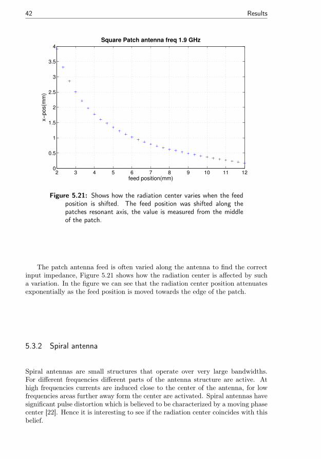
Figure 5.21: Shows how the radiation center varies when the feedposition is shifted. The feed position was shifted along thepatches resonant axis, the value is measured from the middleof the patch.

The patch antenna feed is often varied along the antenna to find the correctinput impedance, Figure 5.21 shows how the radiation center is affected by sucha variation. In the figure we can see that the radiation center position attenuatesexponentially as the feed position is moved towards the edge of the patch.

5.3.2 Spiral antenna

Spiral antennas are small structures that operate over very large bandwidths.For different frequencies different parts of the antenna structure are active. Athigh frequencies currents are induced close to the center of the antenna, for lowfrequencies areas further away form the center are activated. Spiral antennas havesignificant pulse distortion which is believed to be characterized by a moving phasecenter [22]. Hence it is interesting to see if the radiation center coincides with thisbelief.

“output” — 2014/6/18 — 14:52 — page 43 — #51

Results 43

Figure 5.22: Radiation center of the simulated Spiral antenna.

In Figure 5.22 we can see that the radiation center of the simulated spiralantenna is fixed in its center for all frequencies. This does not fit at all with thepredictions for the phase center. This could be due to the fact that the antennaradiates symmetrically up and down, thus the movement inducing effects of theradiation cancel out.

5.4 Endfire dipole arrays

5.4.1 Log-periodic dipole array antenna

The log-periodic antenna is a structure made from dipoles with lengths that varylogarithmically. In contrast to other similar structures, such as the Yagi-Uda an-tenna with one active element, these dipoles are galvanically connected. This givesthe antenna a wide bandwidth as the dipoles are resonant for different frequencies.As a certain dipole starts to resonate the phase center should move closer to it,making the phase center vary across the structure over frequency. The expectedbehaviour of the antenna is thus that the phase center should fall in the region ofthe resonant dipole.

“output” — 2014/6/18 — 14:52 — page 44 — #52

44 Results

Log-periodic antenna

Resonance of first dipole (GHz) 1.93Resonance of last dipole (GHz) 4.68Length (mm) 189.24

Table 5.7: Specification of the simulated Log-periodic antenna.

Figure 5.23: The radiation center of the log-periodic antenna.

The first dipole in this log-periodic antenna is resonant at 1.9 GHz, as seen inTable 5.7. For low frequencies Figure 5.23 shows that the radiation center doesnot correspond to the resonant dipoles position but is shifted towards the otherdipole elements of the antenna. This continues linearly up to high frequencieswhere the radiation center’s position shifts less and less. This behaviour is due tothe resonance in the other elements made stronger by their galvanic connection tothe currently resonant dipole. The smaller antenna elements seem to pull harderon the radiation center than the larger elements do, evident by the fact that theradiation center is shifted a greater distance from its resonant element at lowfrequencies.

“output” — 2014/6/18 — 14:52 — page 45 — #53

Results 45

2 2.5 3 3.5 4 4.50.04

0.06

0.08

0.1

0.12

0.14

0.16

0.18

0.2

Log−periodic antenna

Frequency(GHz)

y−

pos(m

)

radiation center

60o cut phase center



Figure 5.24: A comparison between the radiation center and thephase center as calculated by CST. The HPBW of this antennavaries between 160-90 degrees in the H-plane, and between 79-62 in the E-plane.

The phase and radiation centers agree extremely well in Figure 5.24. Thevarious phase cuts in CST do not make a big difference in the calculation ofthe phase center. This is due to the log periodic antenna having a wide and welldefined main beam which does not change much in shape and size over the antennasoperational frequencies. Thus the CST calculation produce good results, as theydo not include parts of the phase function which correspond to low amplituderadiation.

5.4.2 Yagi-Uda antenna

The Yagi-Uda antenna is a narrow band antenna with high directivity. These goodqualities and its rather simple design mean that Yagi-Uda antennas are widelyused. They consist of a single active element surrounded by parasitic elementsknown as directors and reflectors. There are usually only a few reflectors whichare positioned behind the driven element, these are slightly longer than the activeelement. To the front there are several directors which are slightly shorter thanthe active element. Because of the resonance with these parasitic elements thephase center should not coincide with the active element.

“output” — 2014/6/18 — 14:52 — page 46 — #54

46 Results

Yagi-Uda antenna

Directors 4Reflectors 1Director length (mm) 4Reflector length (mm) 5.2Driven element length (mm) 5Length (mm) 5.7Resonance (GHz) 35.1

Table 5.8: Specification of the simulated Yagi-Uda antenna.

Figure 5.25: Radiation center of the simulated Yagi-Uda antenna.

The radiation center in Figure 5.25 lies within the bounds of the antenna. Wesee that the position is shifted away from the active element as expected.

“output” — 2014/6/18 — 14:52 — page 47 — #55

Results 47

33.8 33.85 33.9 33.95 34 34.05 34.1 34.15 34.2

−1

0

1

2

3

4

5

6

7

8

Last element

Reflector

Driven element

Yagi−Uda antenna

Frequency(GHz)

z−

po

s(m

m)

RC

70o cut PC

60o cut PC

50o cut PC

40o cut PC

30o cut PC

Figure 5.26: A comparison between the phase and radiation centerfor the Yagi-Uda antenna. The HPBW of this antenna is about50 degrees.

Figure 5.26 depicts the differences in the location of the phase and radiationcenters for the Yagi-Uda antenna. The phase center is located far outside theantenna structure which is not impossible, but not predicted. The radiation centeron the other hand lies in a much more realistic region of the antenna.

5.5 Leaky Lens antenna

The specifications of this Lens antenna can be found in [18, 19]. Here the lensantenna is included in this thesis as an example of an advanced antenna structurewhere the phase center position is of interest, but the classical methods fail toprovide feasible answers. The phase center of a lens antenna should fall inside of thestructure, as this is where it has its focus. In Figure 5.27 we see that the radiationcenter meets this expectation. Figure 5.28 shows how the phase and radiationcenter vary with frequency for the leaky lens antenna along its directional axis. Itis clear that the phase center falls well outside the lens antenna, to positions whichare not realistic. This supports the validity of the radiation center calculation asit can produce probable results for this type of antenna.

“output” — 2014/6/18 — 14:52 — page 48 — #56

48 Results

Figure 5.27: The radiation center of the simulated leaky lens an-tenna.

20 25 30 35 40 45 50 55 60 65−0.01

−0.005

0

0.005

0.01

0.015

0.02

0.025

0.03

0.035

0.04

Leaky Lens antenna

Frequency(GHz)

y−

pos(m

)

End of Lens

Bottom of substrate

RC

30o cut PC

20o cut PC

15o cut PC

Figure 5.28: A comparison between the phase and radiation centeralong the main direction of the lens antenna.

“output” — 2014/6/18 — 14:52 — page 49 — #57

Results 49

5.6 Phase comparison

In the previous sections we evaluated the position of the radiation center and thephase center for a set of different antennas. In this section we will look at theactual phase function in the main beam when the far-field has been translatedto the phase or radiation center. This is interesting as the goal of the phase andradiation center is to minimize the phase. For brevity only some of the antennaswill feature in this section. We will only investigate the phase at a single frequencyfor the chosen antennas. This is done in order to get a general sense of how greatthe differences between the centers are.

−10 −5 0 5 10−10

−8

−6

−4

−2

0

2

4

6

8

θ

Pha

se

(deg

ree

s)

E−plane

Square Horn freq 7 GHz

−10 −5 0 5 10−100

−50

0

50

100

150

200

θ

Pha

se

(deg

ree

s)

H−plane

RC

30o cut PC

20o cut PC

10o cut PC

Figure 5.29: A comparison of the phase function inside the HPBW ofthe far-field when translated to the radiation and phase centersfor the square aperture horn antenna.

The phase variation in the E- and H-plane is very different in Figure 5.29,the H-plane phase varies several magnitudes more than the E-plane phase. In theE-plane phase we can clearly see that the 30 cut has the least smooth phase.The thinner phase center cuts have less variation than the radiation center in theE-plane but not necessarily in the H-plane. The 20 cut has the greatest variationin the H-plane where the radiation center seems the smoothest.

“output” — 2014/6/18 — 14:52 — page 50 — #58

50 Results

−10 −5 0 5 10−6

−4

−2

0

2

4

6

8

θ

Ph

ase

(de

gre

es)

E−plane

Square Horn freq 7 GHz

−10 −5 0 5 10−100

−80

−60

−40

−20

0

20

40

60

θ

Ph

ase

(de

gre

es)

H−plane

RC

E/H−plane CST PC

E/H−plane Muehldorf PC

Muehldorf PC

Figure 5.30: A comparison of the phase function inside the HPBWfor the Square horn antenna when it has been minimized by theradiation center,CST phase center and Muehldorf phase center.

The H-plane phase function in Figure 5.30 is very similar for the differentcenters. In the E-plane the magnitude of variation is much less than the H-plane,but the differences between the centers are much more pronounced. The CSTphase function is the most uneven in the E-plane, where as the Muehldorf E-planephase center achieves the smoothest phase. However, the actual differences arevery small, meaning that all centers seem to minimize the phase well.

“output” — 2014/6/18 — 14:52 — page 51 — #59

Results 51

−50 0 50−60

−40

−20

0

20

40

60

θ

Ph

ase

/ d

egre

es

E−plane

Sectoral H−plane horn freq 5 GHz

−10 −5 0 5 10−80

−60

−40

−20

0

20

40

60

θP

hase

/ d

egre

es

H−plane

RC

50o cut PC

40o cut PC

30o cut PC

20o cut PC

Figure 5.31: A comparison of the phase function inside the HPBW ofthe far-field when translated to the radiation and phase centersof the sectoral H-plane aperture horn antenna. Note that theangular width of the HPBW is different in the two planes.

In Section 5.2.3 we showed that the radiation center calculation was influencedby the radiation in the E-plane than the H-plane. For the Sectoral H-plane horn,Figure 5.31 shows that the magnitude of the phase variation is similar in the E-and H-plane. All centers seem to minimize the phase equally in the H-plane. Inthe E-plane the radiation center and the narrower CST cuts seem to minimize thephase well, whereas the wider cuts give more even phase functions.

“output” — 2014/6/18 — 14:52 — page 52 — #60

52 Results

−50 0 50−40

−30

−20

−10

0

10

20

30

40

50

θ

Ph

ase

/ d

egre

es

E−plane

Sectoral H−plane horn freq 5 GHz

−10 −5 0 5 10−80

−60

−40

−20

0

20

40

60

80

θ

Ph

ase

/ d

egre

es

H−plane

RC

E/H−plane RC

E/H−plane CST PC


Figure 5.32: A comparison of the phase function inside the HPBWof the Sectoral H-plane horn when minimized by the radiationcenter, CST phase center and the Muehldorf phase center. Notethat the angular width of the HPBW is different in the twoplanes.

In Figure 5.32 we can see that the E-plane truncated radiation center does notminimize the phase particularly well. The CST E-plane phase center and the totalradiation center seems to minimize the phase most effectively in the E-plane. Noneof the centers seem better or worse at minimizing the phase in the H-plane. Figure5.32 suggests that the truncated radiation center does not achieve its purpose, tominimize a specific phase, particularly well.

“output” — 2014/6/18 — 14:52 — page 53 — #61

Results 53

−20 0 20−2

−1.5

−1

−0.5

0

0.5

1

1.5

2

2.5

3

θ

Ph

ase

/ d

eg

ree

s

E−plane

RC

30o cut PC

20o cut PC

10o cut PC

RC

30o cut PC

20o cut PC

10o cut PC

Log−periodic antenna freq 3 GHz

−40 −20 0 20 40−40

−30

−20

−10

0

10

20

30

θP

ha

se

/ d

eg

ree

s

H−plane

Figure 5.33: A comparison of the phase function inside the HPBW ofthe far-field when translated to the radiation and phase centersof the Log-periodic antenna. Note that the angular width ofthe HPBW is different in the two planes.

The phase variation of in the E-plane of Figure 5.33 is extremely small. Thephase minimized by the radiation center seems to vary the most but still only acouple of degrees. In the H-plane the phase variation is significantly larger butthere is hardly any difference between the centers.

“output” — 2014/6/18 — 14:52 — page 54 — #62

“output” — 2014/6/18 — 14:52 — page 55 — #63

Chapter 6Discussion

Throughout the simulations that have been carried out in this thesis it has beenobvious that the angular momentum method does not consistently produce thesame results as classical phase center calculations. However, it is possible thatthis is purely because the radiation center minimizes the phase better than thephase center. For antennas where the phase center is well defined, e.g. the Log-periodic antenna see Section 5.4.1, the radiation and phase center coincide verywell. For other antennas, such as the Sectoral horn antennas in Section 5.2.3, theCST phase center calculations produce very unstable curves where the radiationcenter varies smoothly. For some antenna structures, the phase center calculationsproduce results far outside of the possible bonds, e.g. the Leaky Lens antenna seeSection 5.5.

One of the most important antennas when discussing the phase center is thehorn antenna, because it is often characterized by its phase center. In Section5.2.1 we notice the radiation center coincides fairly well with CST phase centerresults, as well as Muehldorf calculations for a square aperture horn antenna.However, the rectangular horn antenna is only slightly different from the squarehorn antenna and yet we see much greater differences in Section 5.2.2. Thesedifferences become more prominent as the ratio between the aperture height andwidth is changed further with the sectoral horn antennas in Section 5.2.3. Whenthe difference between the height and the width is increased the width of theradiation lobe increases in the E-plane and decreases in the H-plane. CST onlyallows for one cut angle to be selected when calculating the phase center, thisresults in the calculation ignoring some of the high amplitude radiation in theE-plane. The radiation center calculation on the other hand does not have thisproblem, since it evaluates the entire phase function with the angular momentum.Thus the radiation center’s behavior follows the phase center of the plane withthe widest radiation lobe. Evidence of CSTs single cut angle influencing resultscan be seen elsewhere as well. Specifically, the horn antenna results differ instability. Where the phase center seems to oscillate, particularly when the phasecut is incorrectly chosen, the radiation center produces relatively smooth curvesfor all types of horns. The radiation center does not seem to excel in the truncatedcalculations. The E- and H-plane truncated radiation center does not match thepredicted behaviour of the E- and H-plane phase centers for the sectoral hornantennas in Figures 5.13 and 5.16. The truncated radiation center does not seemto minimize the phase function effectively in Figure 5.32. The general radiation

55

“output” — 2014/6/18 — 14:52 — page 56 — #64

56 Discussion

center minimizes the phase more effectively even though the truncated radiationcenter is only calculated by the radiation in the plane.

For some of the other antennas the results were not as obvious, e.g. the spiralantenna. Previous theories predict that the phase center of the spiral antennashould move with frequency as the spiral antenna has significant pulse distor-tion [22]. The radiation center does not match this prediction at all and is fixedin the center of the antenna for all frequencies. This could be due to the fact thatthe spiral antenna radiates symmetrically from its top and bottom, canceling outany movement of the radiation center. In normal implementation spiral antennasusually feature an absorber on one of their sides in order to only radiate in one di-rection. Such an absorber could lead to a variation in the radiation center position.However, simulating such a structure falls outside the scope of this thesis.

The results from the patch antenna simulations in Section 5.3.1 are not clearcut either. The phase center does not seem to vary with the width of the patchwhereas the radiation center does. This could be due to the difference in how thephase information is extracted. In the CST phase center calculations, see Section4.6.2, the phase function is minimized directly. The radiation center calculationson the other hand minimizes the phase indirectly through the far-field amplitudein Equation (4.4.3). The far-field amplitude is derived directly from the currentson the antenna structure in Equations (4.1.20) and (4.1.16). When the width ofthe patch is changed, the current distribution changes, which could lead to thedifference in radiation center position. Investigating the radiation center’s relationto the surface current falls to future work.

In Section 5.6, we regarded the actual phase function after minimization bythe radiation center and the phase center. These examples are interesting asthey indicate that the radiation center minimizes the phase well in the main lobe.However, in most of the examples the phase center has slightly less variation inthe phase than the radiation center. While such a small range of examples is notenough to draw any final conclusions, they seem to indicate that the radiationcenter fulfills its intended role.

“output” — 2014/6/18 — 14:52 — page 57 — #65

Chapter 7Conclusions

The goal of this thesis was to investigate if the radiation center is a suitablereplacement for the phase center in terms of origin of the radiated field. Forantennas where the phase center is well known, such as the horn antenna, we haveseen the radiation center calculations produce plausible results. We have also seenthe radiation center calculations achieve acceptable results for antennas wherethe phase center methods could not, e.g. the Leaky lens and Yagi-Uda antenna.Additionally the radiation center posseses qualities which the phase center lacks.

The radiation center can be implemented on any antenna structure.For phase center calculations the antenna needs to have a well defined mainbeam, the radiation center calculation on the other and uses the entire sphereof radiation to calculate its position.

The radiation center does not need user input in its calculation.A big disadvantage in current phase center calculations is the need for userinput. The results of the calculation vary wildly with user input, as can beseen in the results presented in Chapter 5.

Finally, when the explicit phase cuts were examined in Section 5.6 we saw thatthe radiation center minimized the phase function in the main lobe almost as wellas the phase center. We can thus conclude that the radiation center is a primecandidate for origin of radiation for antennas.

57

“output” — 2014/6/18 — 14:52 — page 58 — #66

“output” — 2014/6/18 — 14:52 — page 59 — #67

Chapter 8Future work

The work done in this thesis has indicated additional areas of research in investi-gating the radiation center.

Investigating a method for evaluating the smoothness of the phase func-tion.

How do we tell if the radiation or phase center has minimized the phase best?A method of evaluating how well the phase is minimized would greatly helpin determining if the radiation center should replace the phase center.

Further investigation into the effect of angular truncation on the radi-ation center.

Does the radiation center minimize the phase in a plane well if its data istruncated to that plane?

Investigation into the current dependence of the radiation center.

The theory of the radiation center is closely linked to the surface currents ofthe antenna. Investigating this relation could greatly help our understand-ing of the radiation center.

Simulating larger array antennas and calculating the radiation centerof their elements.

In this thesis we were unable to calculate the radiation center of each ele-ment in an array antenna. This would be very interesting to investigate, aswe would be able to see how the resonance between antenna elements in anarray affected their electrical position. The electrical position is importantas it can have a huge impact on sensitive measurements such as Directionof Arrival.

59

“output” — 2014/6/18 — 14:52 — page 60 — #68

60 Future work

Investigate the physical implications of the cot θ term in a1 (4.4.4).

It is unclear what this term represents or if it is unimportant physically.Understanding its presence will further our understanding of what the ra-diation center is.

“output” — 2014/6/18 — 14:52 — page 61 — #69

Chapter 9Appendix

Appendix A Vector Spherical Harmonics

The vector spherical harmonics are defined as,

A1lm(r) =

1√l(l + 1)

∇× (rYlm(r)) =1√

l(l + 1)∇Ylm(r)× r,

A2lm(r) =1√

l(l + 1)r∇Ylm(r),

(A.1)

where τ = 1, 2, l = 1, 2, ...,∞, and m = −l,−l + 1, ..., l. The sphericalharmonics Ylm(r)(θ, φ) are defined as,

Ylm(θ, φ) =

√2l + 1

4π

(l −m)!

(l +m)!Pml (cos θ)ejmφ,

where Pml (cos θ) are the Legendre polynomials [2]. The spherical vectorharmonics and spherical harmonics are orthonormal on the unit sphere Ω,∫∫

Ω

Aτlm(r) ·Aτ ′l′m′(r)dΩ = δττ ′δmm′δll′ ,∫∫Ω

Ylm(r)Yl′m′(r)dΩ = δll′δmm′ .

Appendix B Divergence and Laplace operators

The Laplace and divergence operators on the unit sphere are defined as,∇Ω = rPΩ · ∇ = θ

∂

∂θ+ φ

1

sin θ

∂

∂φ,

∇2Ω =

1

sin θ

∂

∂θ

(sin θ

∂

∂θ

)+

1

sin2 θ

∂2

∂φ2,

(B.1)

where PΩ = I − rr is the projection operator on the unit sphere. Usingthese relations the PΩL2 operator acting on a transverse vector field F canbe calculated using the definition of the Laplace operator [7],

∇2F (r) = ∇(∇ · F )−∇× (∇× F ). (B.2)

61

“output” — 2014/6/18 — 14:52 — page 62 — #70

62 Appendix

By using the definitions of the divergence and rotation in spherical coordi-nates [2] equation B.2 can be expanded:

∇(∇ · F ) = r

(−∂Fθ∂θ− Fθ

cos θ

sin θ− 1

sin θ

∂Fφ∂φ

)+θ

(∂2Fθ∂θ2

+ cot θ∂Fθ∂θ− (1− cot2 θ)Fθ +

1

sin θ

∂2Fφ∂φ∂θ

− cos θ

sin2 θ

∂Fφ∂φ

)+φ

(1

sin θ

∂2Fθ∂φ∂θ

+cos θ

sin2 θ

∂Fθ∂φ

+1

sin2 θ

∂2Fφ∂φ2

)(B.3)

∇× (∇× F ) = r

(∂Fθ∂θ

+ cot θFθ +1

sin θ

∂Fφ∂φ

)+θ

(1

sin θ

∂2Fφ∂φ∂θ

+cos θ

sin2 θ

∂Fφ∂φ− 1

sin2 θ

∂2Fθ∂φ2

)+φ

(−∂

2Fφ∂θ2

− cot θ∂Fφ∂θ

+ (1 + cot2 θ)Fφ +1

sin θ

∂2Fθ∂φ∂θ

− cos θ

sin2 θ

∂Fθ∂φ

)(B.4)

Combining Equation (B.3) and (B.4) according to Equation (B.2) and usingthe definitions in Equation (B.1) leads to the following expression for thesquared angular momentum operator PΩL2,

PΩL2F (r) = θ

(−∇2

ΩFθ +Fθ

sin2 θ+

2 cos θ

sin2 θ

∂Fφ∂φ

)φ

(−∇2

ΩFφ +Fφ

sin2 θ+

2 cos θ

sin2 θ

∂Fθ∂φ

).

(B.5)

Finally we recognise the ∇2Ω operator from Equation (B.1),

L2F (r) = −∇2ΩF (r).

Appendix C Product rules for angular momentum

The ∇2 operator acing upon two vector fields is calculated as

∇2(ΦΨ) = ∇ · ∇(ΦΨ) = ∇ · (Ψ∇Φ + Φ∇Ψ) = 2∇Ψ · ∇Φ + Φ∇2Ψ + Ψ∇2Φ.

The same principle can be applied to a tangential vector field F , when itis regarded in its Cartesian components,

∇2(FΨ) = 2∇Ψ · ∇F + F∇2Ψ + Ψ∇2F . (C.1)

The projection operator is expanded by its definition [2] as,

∇2Ω(FΨ) = r × (r ×∇2(FΨ)). (C.2)

“output” — 2014/6/18 — 14:52 — page 63 — #71

Appendix 63

Combining Equations (B), (C.2) and (C.1) the squared angular momentumcan be written as

L2(FΨ) = r × (r × (2∇Ψ · ∇F + F∇2Ψ + Ψ∇2F )

= FL2Ψ + ΨL2F + r × (r × (2∇Ψ · ∇F )).(C.3)

Hence only the last term needs further investigation,

r2∇Ψ · ∇F =∂Ψ

∂θ

∂

∂θ(θFθ + φFφ) +

1

sin2 θ

∂Ψ

∂φ

∂

∂φ(θFθ + φFφ) (C.4)

By using the coordinate transformation relations [7] to cartesian coordinatesone can easily prove the following relations,

∂θ

∂θ= −r,

∂φ

∂θ= 0,

∂θ

∂φ= −φ cos θ,

∂φ

∂φ= −ρ = −r sin θ − θ cos θ.

Which are used to rewrite equation C.4,

r2∇Ψ · ∇F =− ∂Ψ

∂θrFθ +

1

sin2 θ

∂Ψ

∂φ(φ cos θFθ − (r sin θ + θ cos θ)Fφ)

+∂Ψ

∂θ

(θ∂Fθ∂θ

+ φ∂Fφ∂θ

)+

1

sin2 θ

∂Ψ

∂φ

(θ∂Fθ∂φ

+ φ∂Fφ∂φ

).

(C.5)

This equation can then be put back into Equation C.4to make the followingsimplification,

r × (r × (2∇Ψ · ∇F )) =− 2cos θ

sin2 θ

∂Ψ

∂φ

(φFθ − θFφ

)− 2

∂Ψ

∂θ

(θ∂Fθ∂θ

+ φ∂Fφ∂θ

)− 2

sin2 θ

∂Ψ

∂φ

(θ∂Fθ∂φ

+ φ∂Fφ∂φ

),

=− 2cos θ

sin2 θ

∂Ψ

∂φr × F − 2

(θ∇ΩFθ + φ∇ΩFφ

)· ∇ΩΨ.

(C.6)

Thus using C.6 and C.3 the product can finally be written as:

L2(FΨ) = FL2Ψ+ΨL2F−2cos θ

sin2 θ

∂Ψ

∂φ(r×F )−2(θ∇ΩFθ+φ∇ΩFφ)·∇ΩΨ (C.7)

Appendix D Translation of the far-field

Translation of the origin of the far-field can be expressed mathematically as

F (r)→ F (r)e−jk·d.

“output” — 2014/6/18 — 14:52 — page 64 — #72

64 Appendix

Hence in the calculation of the squared angular momentum the productrules from appendix C become applicable,

L2(F (r),d) =

∫∫Ω

F ∗(r)ejk·d · PΩL2F (r)e−jk·ddΩ. (D.1)

The product rule for squared angular momentum acting on a vectorfieldand a scalar field is given in (C.7). In this case Ψ = e−jk·d, the derivativesof Ψ in (C.7) then become,

∂Ψ

∂θ= −jkθ · de−jk·d,

∂Ψ

∂φ= −jkφ · d sin θe−jk·d,

∇ΩΨ = −jk[θθ + φφ

]· de−jk·d,

L2[Ψ] = −j2kr · de−jk·d + k2[(θ · d)2 + (φ · d)2

]e−jk·d.

(D.2)

Using these derivatives (C.7) can be rewritten as,

L2(F e−jk·d) =F(−j2kr · d+ k2

[(θ · d)2 + (φ · d)2

])+ L2F + j2k cot θφ · d(r × F )

+j2k(θ∇ΩFθ + φ∇ΩFφ) ·[θθ + φφ

]· dejk·d.

This expression is then put into (4.4.3) to get the translated squared angularmomentum,

L2(F (r),d) =

∫∫Ω

(F ∗ · L2F ) + (F ∗ · F )

(k2[(θ · d)2 + (φ · d)2

])− j2k

((F ∗ · F )(r · d)− cot θr · (F × F ∗)(φ · d)

−(F ∗θ∇ΩFθ + F ∗φ∇ΩFφ) ·[θθ + φφ

]· d)

dΩ.

Finally the expression can be rewritten to a more compact form,

L2[F (r),d] = a0 + 2ka1 · d+ k2d ·A2 · d, (D.3)

where

a0 =L2(F (r), 0) =

∫∫Ω

F ∗ · L2FdΩ,

a1 =− j

∫∫Ω

(F ∗ · F )rdΩ + j

∫∫Ω

[F ∗θ∇ΩFθ + F ∗φ∇ΩFφ]dΩ

+ j

∫∫Ω

cot θr · (F × F ∗)φdΩ,

A2 =

∫∫Ω

(F ∗ · F )[θθ + φφ]dΩ.

(D.4)

“output” — 2014/6/18 — 14:52 — page 65 — #73

Appendix 65

a1 can be further rewritten to show that it is in fact a real valued quantity.If Gauss theorem on the unit sphere [23, (A3.45)],∫∫

Ω

u(r)rdΩ =1

2

∫∫Ω

∇Ωu(r)dΩ, (D.5)

is applied to the first integral in a1 we get:

−j

∫∫Ω

(F ∗ · F )rdΩ = − j

2

∫∫Ω

∇Ω(F ∗ · F )dΩ

= − j

2

∫∫Ω

[Fθ∇ΩF∗θ + Fφ∇ΩF

∗φ + F ∗θ∇ΩFθ + F ∗φ∇ΩFφ]dΩ.

Which when combined with the second integral in a1 becomes,

− j

2

∫∫Ω


∗φ − (F ∗θ∇ΩFθ + F ∗φ∇ΩFφ)]dΩ

= − j

2

∫∫Ω


∗φ − (Fθ∇ΩF

∗θ + Fφ∇ΩF

∗φ )∗]dΩ

=

∫∫Ω


∗φ ]dΩ. (D.6)

The last integral in a1 can be written as,

j

∫∫Ω

cot θr · (F (r)× F ∗(r))φdΩ = −2

∫∫Ω

cot θ Im(FθF∗φ )φdΩ, (D.7)

by explicitly calculating the cross product and projection with regards tothe fields angular components. Thus when (D.6) and (D.7) are used tosimplify a1 it is more apparent that a1 is real-valued,

a1 =

∫∫Ω


∗φ ]dΩ− 2

∫∫Ω

ImFθF ∗φdΩ.

Now only the A2 term in (D.4) remains to be analyzed to prove that all thequantities are positive and real valued. This can be seen by multiplying itby an arbitrary real vector d = dd,

d ·A2 · d = d2

∫∫Ω

F ∗ · F [(d · θ)2 + (d · φ)2]dΩ > 0. (D.8)

Thus all quantities in (D.4) are positive real valued or positive definite andcan be written as,

a0 =L2(F (r), 0) =

∫∫Ω

F ∗ · L2F dΩ,

a1 =

∫∫Ω


∗φ ] dΩ− 2

∫∫Ω

ImFθF ∗φ dΩ,

A2 =

∫∫Ω

(F ∗ · F )[θθ + φφ] dΩ.

“output” — 2014/6/18 — 14:52 — page 66 — #74

66 Appendix

Appendix E Euler rotations

Euler angles are three angles that can create all rotations of an object inthree dimensional space. The rotation operator based on these angles isgiven by

R(α, β, γ) =

cos γ cosα− cosβ sinα sin γ cos γ sinα+ cosβ cosα sin γ sin γ sinβ− sin γ cosα− cosβ sinα cos γ − sin γ sinα+ cosβ cosα cos γ cos γ sinβ

sinβ sinα − sinβ cosα cosβ

Appendix F Simulations

The results in this thesis have been simulated using the software CST andanalysing the results in Matlab. In Matlab, Ericsson Antenna Model Librarytoolbox has been used. CST is a powerful program used to simulate variousstructures including antennas. In this essay it’s main use was to simulate thefar-field of an antenna for a given frequency. The far-field is then exportedto Matlab where the phase center calculations can be done with the eamlibtoolbox.

F.1 Automating CST simulations through Matlab

Far-field data is normally not something that is simulated and exported formany different frequencies at once in CST; usually the field is only simulatedfor the antenna at resonance. Because of this and the fact that the far-fieldtakes some time to simulate there is no easy way to export large amountsof far-field data from CST. The simulations done in this thesis required thefull far-field for each measured frequency to determine the radiation centerat that frequency. The method used to extract this data was based aroundrunning a separate CST session for each frequency. This was achieved byconstructing a for loop in Matlab which created a text file specifying theparameters to be run in CST. Matlab then executed the dos-command torun CST and extracted the results. To do this some steps need to be takento prepare the CST file which will be simulated.

1. Setup a far-field monitor which calculates the far-field at a CST variable’freq’.

2. Run the simulation once and make sure that the far-field is displayed in thedesired way by going to plot properties, e.g. E-field, linear scaling and originin origo.

3. Open the Template based postprocessing window and create two tasks, "Ex-port Farfields as Source" and "Result Storage.sdb". There are two dropdown menus, the first selects your category and the second your task. Tocreate a "Export Farfield as Source" task select the category "Farfield andAntenna Properties". When this is done an option window will appear, se-lect the export format "ASCII .txt" and make sure the excit. string referes

“output” — 2014/6/18 — 14:52 — page 67 — #75

Appendix 67

to the correct far-field monitor. "Result Storage.sdb" is found in the "Misc"category and should be created without changing any default options.

F.2 Simulating single off center elements

CST is not designed to simulate elements that are moved around in referenceto a fixed point. To get accurate results in CST the bounding box volumearound the simulated point has to be large. The best way to ensure this isto have the bounding box be symmetric around the chosen point. When anelement is moved off center the bounding box follows the element. Becauseof this an extra trick is needed to get accurate results. The bounding box iscalculated to encapsulate objects in CST, in order to extend it more objectsmust be added. Since we do not want to change the simulations in anyother way than to extend the dimensions of the bounding box these objectsare chosen to be composed of vacuum. When CST performs a simulation itfills the area around the structure with vacuum, thus adding objects madeof vacuum will not change the simulations.

The simulations in the thesis calculate the far-field in origo. When theantenna element is moved off center an inverted version of the same ele-ment made of vacuum is defined to extend the bounding box symmetricallyaround origo. Both these elements are then translated in opposite directionsif further displacement is needed.

“output” — 2014/6/18 — 14:52 — page 68 — #76

“output” — 2014/6/18 — 14:52 — page 69 — #77

References

[1] IEEE145-1993. IEEE standard definition of terms for antennas, March 1993.

[2] G. Arfken. Mathematical Methods for Physicists. Academic Press, Orlando,third edition, 1985.

[3] C. A. Balanis. Modern Antenna Handbook. John Wiley & Sons, Inc., 2008.

[4] J. Friden and G. Kristensson. Calculation of antenna radiation center us-ing angular momentum. In Antennas and Propagation (EuCAP), 2013 7thEuropean Conference on, pages 1531–1535, April 2013.

[5] J. Fridén and G. Kristensson. Calculation of antenna radiation center usingangular momentum. Technical Report LUTEDX/(TEAT-7219)/1–23/(2012),Lund University, Department of Electrical and Information Technology, P.O.Box 118, S-221 00 Lund, Sweden, 2012. http://www.eit.lth.se.

[6] H. Goldstein. Classical Mechanics. Addison-Wesley, Reading, MA, USA,second edition, 1980.

[7] D. J. Griffiths. Introduction to Electrodynamics. Prentice-Hall, Inc., Engle-wood Cliffs, New Jersey, third edition, 1999.

[8] J. Hald, J. E. Hansen, F. Jensen, and F. Holm Larsen. Spherical Near-FieldAntenna Measurements, volume 26 of IEE electromagnetic waves series. PeterPeregrinus Ltd., 1998. edited by J.E. Hansen.

[9] J. E. Hansen, editor. Spherical Near-Field Antenna Measurements. Num-ber 26 in IEE electromagnetic waves series. Peter Peregrinus Ltd., Stevenage,UK, 1988. ISBN: 0-86341-110-X.

[10] Y. Y. Hu. A method of determining phase centers and its application toelectromagnetic horns. Journal of the Franklin Institute, 271, 31 – 39, 1961.

[11] J. D. Jackson. Classical Electrodynamics. John Wiley & Sons, New York,second edition, 1975.

[12] R. C. Johnson. Antenna Engineering Handbook. McGraw-Hill, New York,third edition, 1993.

[13] G. Kristensson. Spridningsteori med antenntillämpningar. Studentlitteratur,Lund, 1999. (In Swedish).

69

“output” — 2014/6/18 — 14:52 — page 70 — #78

70 References

[14] Y. T. Lo and S. W. Lee. Antenna Handbook Theory, Applications and Design.Van Nostrand Reinhold, New York, first edition, 1988.

[15] T. A. Milligan. Modern Antenna Design, Second Edition. John Wiley & Sons,2005.

[16] P. M. Morse and H. Feshbach. Methods of Theoretical Physics, volume 2.McGraw-Hill, New York, 1953.

[17] E. I. Muehldorf. The phase center of horn antennas. Antennas and Propaga-tion, IEEE Transactions on, 18(6), 753–760, 1970.

[18] A. Neto. UWB, non dispersive radiation from the planarly fed leaky lensantenna-part I: Theory and design. IEEE Trans. Antennas Propagat., 58(7),2238–2247, 2010.

[19] A. Neto, S. Monni, and F. Nennie. UWB, non dispersive radiation from theplanarly fed leaky lens antenna-part II: Demonstrators and measurements.IEEE Trans. Antennas Propagat., 58(7), 2248–2258, 2010.

[20] P. Padilla, J. M. Fernández, J. L. Padilla, G. Expósito-Domínguez, M. Sierra-Castaner, and B. Galocha. Comparison of different methods of the experimet-nal antenna phase center determination using a planar acquisition system.Progess In Electromagnetics Research, 135, 331–346, 2013.

[21] J. J. Sakurai. Modern Quantum Mechanics. Addison Wesley, 1985.

[22] H. G. Schantz. Dispersion and uwb antennas. 2004 International Workshopon Ultra Wideband Systems, Joint with Conference on Ultrawideband Systemsand Technologies. Kyoto, Japan. May 18-21, pages 161–165, 2004.

[23] J. G. Van Bladel. Electromagnetic Fields. IEEE Press, Piscataway, NJ, secondedition, 2007.

[24] P. D. P. W. V. T: Rusch. Analysis of reflector antennas. Academic press, inc.(London) LTD., 1970.

Investig

ation

and

Co

mp

arison

Betw

een R

adiatio

n an

d Ph

ase Cen

ter for C

ano

nical A

nten

nas

Department of Electrical and Information Technology, Faculty of Engineering, LTH, Lund University, June 2014.

Investigation and Comparison Between Radiation and Phase Center for Canonical Antennas

Casimir Ehrenborg

http://www.eit.lth.se

Ca

simir Eh

ren

bo

rg

Master’s Thesis

Documents

Investigation and Comparison Between Radiation and Phase